Article

Defect Identification of Concrete Piles Based on Numerical Simulation and Convolutional Neural Network

1
School of Economics and Management, Chongqing Jiaotong University, Chongqing 400074, China
2
School of Civil Engineering, Chongqing Jiaotong University, Chongqing 400074, China
3
School of Management Science and Real Estate, Chongqing University, Chongqing 400044, China
4
School of Civil Engineering and Architecture, Jishou University, Zhangjiajie 427000, China
*
Author to whom correspondence should be addressed.
Buildings 2022, 12(5), 664; https://doi.org/10.3390/buildings12050664
Submission received: 12 April 2022 / Revised: 7 May 2022 / Accepted: 13 May 2022 / Published: 17 May 2022
(This article belongs to the Special Issue Advanced Methodologies and Technologies in Structural Monitoring)

Abstract

:
Defects in pile foundations, such as neck defects, bulge imperfections, weak concretes, cracks, and broken piles, can cause a decrease in the bearing capacity and the structural stability of the foundation. Identification of the type of defect is vital in formulating a reasonable repair plan for the pile foundation. In this study, the authors proposed a scheme to identify the types of defects in concrete piles based on a convolution neural network and a low-strain pile integrity test (LSPIT). A batch modeling method of defective pile foundations using Python script was also proffered. The different degrees of signals of five types of defective pile foundations were simulated by this method. The original data were decomposed and reconstructed by wavelet packet decomposition (WPT). To prevent the data from losing too much information after WPT, the data of 400 × 1 after decomposition and reconstruction were processed by dimension-raising to obtain the data of 20 × 20 × 1. Then, the multidimensional feature index of 20 × 20 × 2 was generated by index fusion with the original data. Finally, the data were input onto convolutional neural network (CNN) as a training parameter. Following an improvement of the dataset, the recognition accuracy of the type of defect in the pile foundation by the proposed identification scheme reached 94.4%.

1. Introduction

Pile foundations are a widely used form of deep foundation which are often used in important structures such as high-rise buildings, bridges, and ports. Their construction quality and integrity play a very important role in ensuring the overall quality and safety of construction projects. Since the cast-in-place pile is usually formed underground, it has the characteristics of difficult construction, complex process, and ease of concealment. In the construction process, it is easy to produce holes, cracks, interlayers, necking, and other defects, thereby damaging the integrity of the pile. Therefore, using a reasonable and reliable method to detect pile defects is necessary to ensure building safety. Many nondestructive evaluation (NDE) methods can reliably evaluate pile integrity, such as the low-strain pile integrity test (LSPIT), high-strain pile integrity test (HSPIT), cross-hole ultrasonic logging (CSL), single-hole ultrasonic logging (SSL), and gamma ray density logging (GDL) [1]. Among them, the LSPIT is the most commonly used pile detection method in engineering and has the benefits of fast detection and being economical and non-destructive [2]. When this method is used, a force bar or hand hammer is used to strike the top of the pile, and a stress wave is excited to propagate downward along the pile body. In the process of propagation, the stress wave reflects when it encounters defects such as necking of the pile section, segregation, or breaking of the pile, which manifest as changes in wave impedance. The reflected signal is received by a sensor installed at the top of the pile (velocity type or acceleration type). The defects of the pile body are judged by comprehensive analysis of the reflection wave’s time history curve [3]. At present, there are two common methods to detect pile integrity based on reflected wave signals: one is the manual detection method; the second, the pattern recognition method, is based on machine learning [4,5,6]. When the detection signal is interpreted manually, the inspectors must have a very rich experience; have a good knowledge of wave propagation theory, soil mechanics, and piling construction technology; and have a good understanding of LSPIT itself. Therefore, the interpretation of LSPIT signals can only be carried out by experienced experts. For foundation construction sites where the number of piles to be tested is large, it may take days before the expert can complete interpreting all of the piles and deliver the integrity assessment report [7].
At present, there are many studies on the intelligent interpretation of LSPIT signals, such as Yan, T.N., who transforms the time domain signal of LSPIT into a frequency domain signal by fast Fourier transformation and then trains a BP neural network by frequency domain signal to realize intelligent identification of pile defects. However, the damage index only considers the frequency domain characteristics and cannot fully reflect the pile defects [8]. Cai, Q.Y. used wavelet analysis to extract the power spectrum of the LSPIT time domain signal and input it into a BP neural network as a damage characteristic index to achieve the intelligent identification of pile defect types. However, the data set used for training was too small, and the trained classifier cannot be widely popularized [9,10]. Wang, C.H. trained a BP neural network model based on the LSPIT signal waveform curve, pile geometry size, and stress wave propagation speed in the pile and achieved the intelligent identification of pile defect types. However, too many feature types are selected, increasing the parameters of feature recognition and resulting in a slower convergence rate of the neural network [11]. Liu, M.G. uses wavelet analysis to extract the four-layer power spectrum of the LSPIT signal to form a feature vector, which is then input into a BP neural network for training to achieve the intelligent identification of pile defect types. However, the data set used for the training model was too small to be widely promoted [12]. Zhang, G. uses wavelet analysis and a neural network. They use the extreme point of LSPIT signal obtained by wavelet analysis as the input of the neural network and determined the type and location of defects according to the output coding. However, the training data set in this study was too small, and too many useful features were lost in the data processing, so the recognition effect cannot be promoted [13]. Eftychios Protopapadakis used a genetic optimized neural network detector, coupled finite element method, and scale boundary finite element method to model the pile and its surrounding soil. Through data processing technology, multiple characteristic indexes are coupled as damage identification indexes. A neural network model that can identify the type and location of pile defects is obtained by training, but the paper only considers the coupling of two types of defects [14]. Kang, W. used wavelet packet transformation to extract three higher-order statistical parameters in the LSPIT time domain signal: variance, skewness, and kurtosis. After further data processing, the support vector machine model was trained, and finally, a model used to identify the type of pile damage was obtained. However, the parameters used for training were too few, and the classification model is difficult to popularize [15]. Cui, D.M. amplified the LSPIT signals exponentially and then filtered the amplified data by WPT. The processed data were used as the characteristic index for training an ELM neural network. Finally, a model that can be used to explain the defect of the pile foundation was obtained [7]. At present, there are few studies on the intelligent identification of LSPIT signals using convolutional neural networks (CNN), but CNNs have been widely used in the identification of other types of structural damage signals. For example, Vu, G. used numerical simulation to obtain the ultrasonic signal of three types of cracks in concrete. In the data processing, 40,000 × 1 one-dimensional data were converted to 200 × 200 two-dimensional data, and the data were refined. The processed data were used as a damage index to train a convolutional neural network model. Finally, a neural network model that can identify three types of cracks was obtained [16]. Xie, Y. used the empirical model and Hilbert transform to process the vibration signal of the pipeline to obtain the time–frequency map and used it as a feature index to train a convolutional neural network. Finally, a model that can intelligently identify pipeline damage was obtained [17]. Zhuo D.B. used a wavelet transform to convert the acoustic signal of bolt loosening into the wavelet time–frequency diagram and used it as the characteristic index to train the CNN classifier in order to obtain a neural network model for intelligent identification of bolt loosening [18].
Recently, researchers have performed a large amount of research using machine learning to detect damage. Ritto, T.G. constructed structural damage sample data through the digital twin model to train machine learning classifiers and explored the structural detection scheme of digital twins combined with machine learning [19]. Karvelis, P. used acoustic signals to train a machine learning classifier and proposed an SHM method based on machine learning that can locate the positions of defects in real time on a ship [20]. Rautela, M. combined two-level damage identification, viz damage detection, and localization for a composite panel through two neural network models trained by ultrasonic guided wave signals [21]. Perry, B.J. proposed a method to identify bridge damage with an image training machine learning model [22]. Li, Z. simulated the damage model of semi-grouting sleeve with finite element technology, trained a CNN with one-dimensional guided wave signals obtained from numerical simulation, and proposed a model that can detect the defects of semi-grouting sleeve [23].
This paper proposed a method for intelligent identification of defect types of concrete piles using LSPIT signals. Through Python script and finite element software, the different defect degree signals of five common concrete pile defect types were generated regularly. The collected speed signals were further processed by WPT, and a data enhancement method of dimension-up data structure was discussed. Firstly, the one-dimensional velocity signal of 400 × 1 and the WPT reconstruction signal of 400 × 1 were recombined into the two-dimensional data of 20 × 20 × 1, and then the two-dimensional data with a spatial structure relationship were overlapped into 20 × 20 × 2 and input into the CNN as the characteristic index. This data processing operation improves the performance and robustness of the CNN classifier.

2. Method

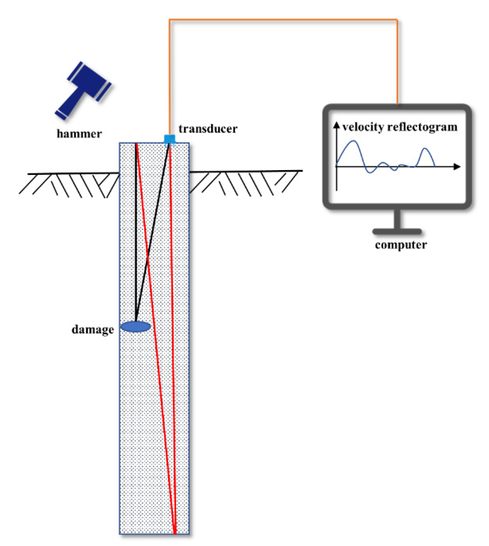
2.1. Low-Strain Pile Integrity Test

LSPIT, also known as pulse echo, acoustic echo, impulse response, or impact echo, is a very convenient nondestructive testing technology widely used in pile integrity testing. With the research of Professor Goble and Ohio Highway Administration, the low-strain pile integrity test has been widely used since the 1970s [24,25]. It is called the “low-strain test” because this technology only induces low stress at the top of the pile and can start a stress wave in the pile. Since the excitation force is very small and the variation of density and elastic modulus of the pile and soil was very small during the LSPIT test, the pile is always in an elastic strain state. The propagation of stress waves can be explained by a one-dimensional equation [26]. The ASTM.D5882 has standardized the low strain pile integrity test and stipulated two testing methods: the pulse-echo method and the transient response method [27]. In this study, we only focus on the transient response method. The stress wave was generated by the transient impact on the pile. By analyzing the propagation of the stress wave, the defect of the pile foundation can be identified. As shown in Figure 1, during the integrity testing of low-strain piles, researchers generate stress waves at the top of the pile by hammering and collecting the propagation of stress waves inside the pile through the velocity sensor placed at the top of the pile.
During the low strain pile integrity test, the stress wave generated by the hammer travels through the pile to obey the one-dimensional wave equation in ideal conditions so that we can recognize this wave through the following equations.
Assuming the pile’s Young’s modulus is E , The cross-sectional area of the pile is A, and the material density of the pile is ρ . Under the excitation force, the displacement of the unit in the pile is expressed as u . The speed of the unit in the pile can be explained as V = u / t ; at the same time, the strain of the pile can be explained as ε = u / x . The propagation velocity of the stress wave is c = E / ρ . At this time the pile is in the elastic deformation stage, following Hooke’s law. According to Newton’s second law and Hooke’s law, the one-dimensional wave equation can be expressed by Equation (1).
2 u t 2 c 2 2 u x 2 = 0
Solving wave Equation (1) can give Equation (2). Through Equation (2), the time domain curve of pile vibration velocity required for low-strain reflection wave method detection can be obtained. The defects of the pile can be determined using the characteristics of the curve, which is our current low-strain reflection wave method commonly used theoretical basis [28].
V ( z , t ) = 1 2 | φ t ( x c t ) c φ 1 ( x c t ) | + 1 2 | φ t ( x + c t ) + c φ 1 ( x + c t ) |

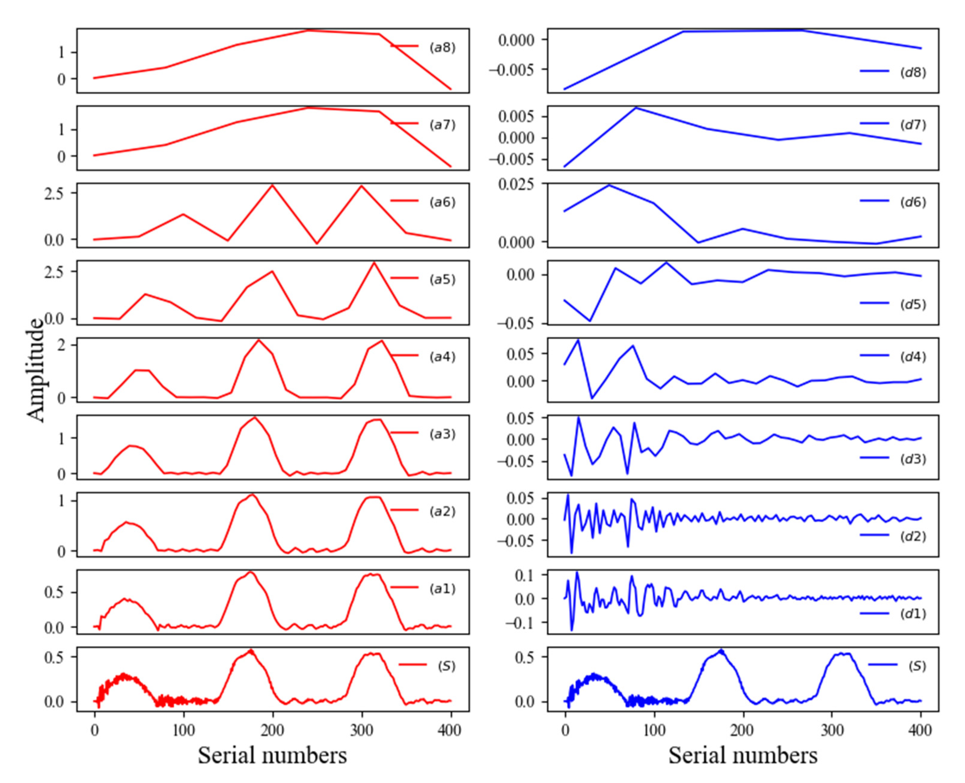
2.2. Wavelet Packet Decomposition

The emergence of WPT gives researchers a new way to analyze signals. Researchers can process signals from multiple perspectives, such as time–frequency analysis, signal–noise separation, weak signal extraction, signal recognition, and diagnosis [25]. Powerful functionality makes wavelet transform adaptable to a large number of situations in signal analysis. Yuan, Q. created a time–frequency analysis of electroencephalogram EEG signals by wavelet transform [29]. Han, J.G. decomposed the structural damage vibration signal of the beam to a wavelet energy index and made it an indicator for damage identification [30]. Bettayeb F performed signal decomposition and reconstruction using wavelet transform in ultrasonic testing of welds [31]. Through WPT, researchers can multilayer high-frequency and low-frequency decomposition of signals, as shown in Figure 2. In most signal analyses, high-frequency signals are often useless noise signals, while low-frequency signals can reflect important information in the signal. Through using the wavelet packet tool to reconstruct the useful frequency signal, signal denoising and filtering can be achieved.
The wavelet packet function is a time–frequency function that can be defined as [25,32].
W i , k n ( t ) = 2 j 2 W n ( 2 j t t k )
where j and k are the scale and translation operations of the wavelet function, respectively; n is the number of decomposition layers. Equations (4) and (5) respectively give the scaling and mother wavelet functions of the wavelet function.
W o , o o ( t ) = ( t )
W o , o 1 ( t ) = ψ ( t )
When the number of decomposition layers n is greater than 1, the wavelet packet’s decomposition of high-frequency and low-frequency signals can be defined by the following formulas, in which h(k) and g(k) are low-pass filters and high-pass filters, respectively.
W o , o 2 n ( t ) = 2 k h ( k ) W 1 , k n ( 2 t k )
W o , o 2 n + 1 ( t ) = 2 k g ( k ) W 1 , k n ( 2 t k )
where the wavelet packet coefficient W j , k n is defined as:
W i , k n = f ( t ) , W i , k n = f ( t ) W i , k n ( t ) d t

2.3. Finite Element Analysis of Pile

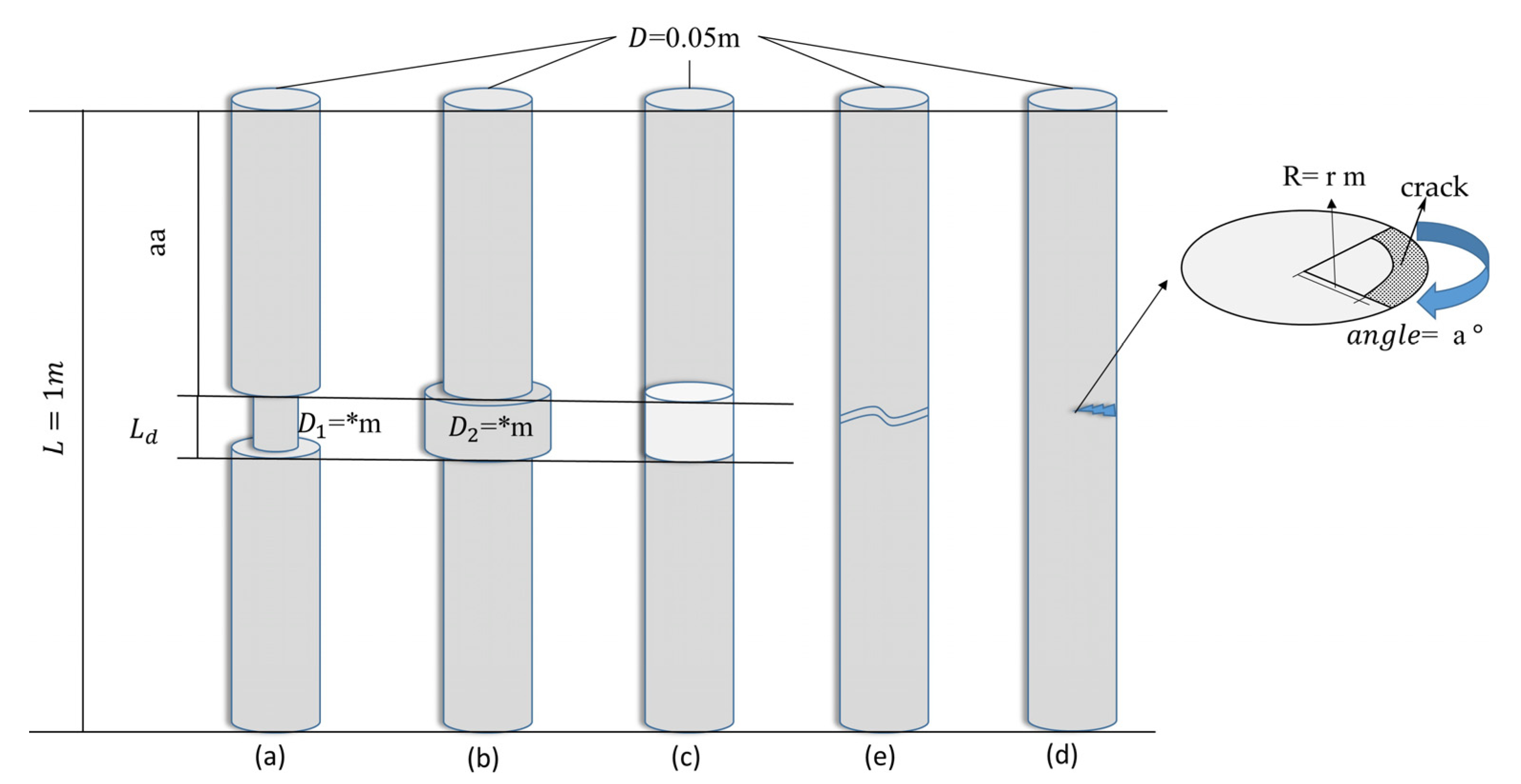
2.3.1. Basic Theory and Modeling Parameters

In classifier training, a large number of defective pile signals were needed for training. However, in practical research, it is not easy to obtain such defective data. It is impossible to obtain enough defective pile data only through actual experiments. Therefore, this study used finite element software to simulate defective piles to obtain a large number of sample signals of defective piles.
During the experiment, due to the variation of density, the elastic modulus of the pile and soil was very small. Therefore, it can be considered that the result of the low strain signal was directly related to the geometric shape of the piles. The defect type studied in this paper can be considered linear damage, which is defined as the case in which the initial linear elastic structure remains linear after damage [14,33,34,35].
Therefore, only defects in the pile under ideal conditions were considered; that is, when the pile and soil were both in the linear elastic state, the material of the pile body was uniform, only the case of a single defect of the pile body was considered, and the length and radius of the pile and the soil around the pile remained unchanged. Based on these conditions, this paper carried out different degrees of simulation experiments on the common defect types of pile foundation such as neck defects, bulge imperfections, weak concrete, cracks, and broken piles, as shown in Figure 3. Research has shown that three-dimensional finite element analysis has the same accurate calculation results as one-dimensional finite element analysis [36,37]. In this study, the finite element analysis software ABAQUS was used to conduct a simulation test of integrity detection for low-strain pile foundations [38].
Parameters of pile and soil are shown in Table 1. Through calculation, it can be seen that the propagation velocity of the stress wave in the pile is 3464 m/s, and the propagation velocity in the soil is 154 m/s. The radius of soil around the pile was set to 10 times the radius of the pile, and the length of the soil at the bottom of the pile was 1/2 of the length of the pile. During the analysis step time, the reflected wave of the soil boundary around the pile cannot be reflected to the sensor, which affects the reflected wave in the pile [39,40,41]. According to the experimental results of Cook, when the diameter of the soil around the pile reaches 10 times the diameter of the pile, the shear displacement can be ignored [42].
In this study, when the wave can pass through 10 elements within the action time of impact load, the wave propagation along the pile can be seen in the signal. By calculation, when the unit size is less than 0.05 m, the wave propagation can be seen along with the pile [38]. The modeling in this study is based on linear damage and only cares about the displacement of the unit. Since C3D8R (three-dimensional eight-node reduced integral element) is a common finite element in ABAQUS (Standard version 2019, distributed by SIMULIA Inc., Toulouse, France) and is more accurate in calculating the displacement of the model, the model was modeled by C3D8R, which can meet the research requirements [38]. Since C3D8R must be sufficiently small to obtain better calculation results, the unit size of the pile was set to 0.003 m to obtain more accurate results.
Analysis step time is 0.0012 s. Boundary conditions: the soil around the pile was fixed in X and Y directions (U1 = U2 = 0); the pile bottom is fixed in X, Y, and Z directions (U1 = U2 = U3 = 0), and no restraint was imposed on the top of the pile. The explicit integration method (ABAQUS/Explicit) was used for modeling. This method is especially applicable in the case of instantaneous motion, such as impact load. Many small increments were required to obtain a high-resolution solution. The basic modeling parameters are shown in Table 1.

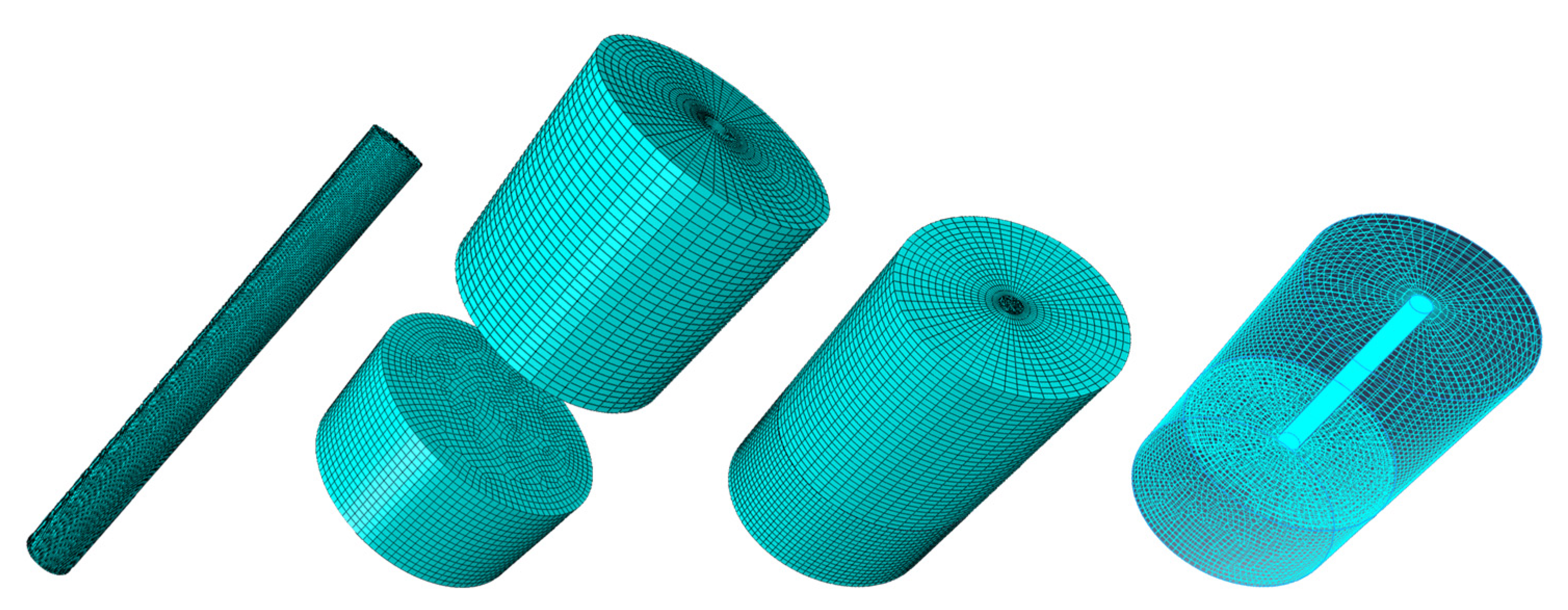
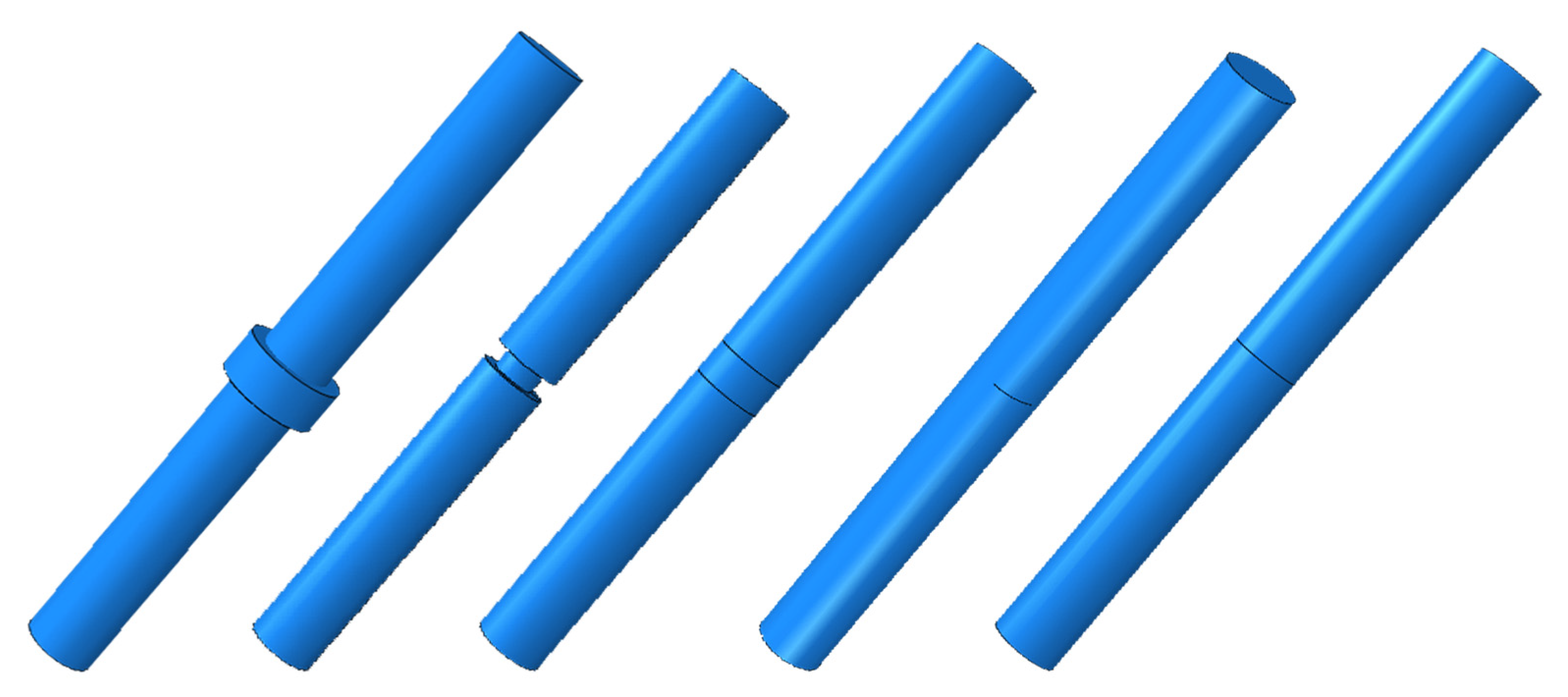
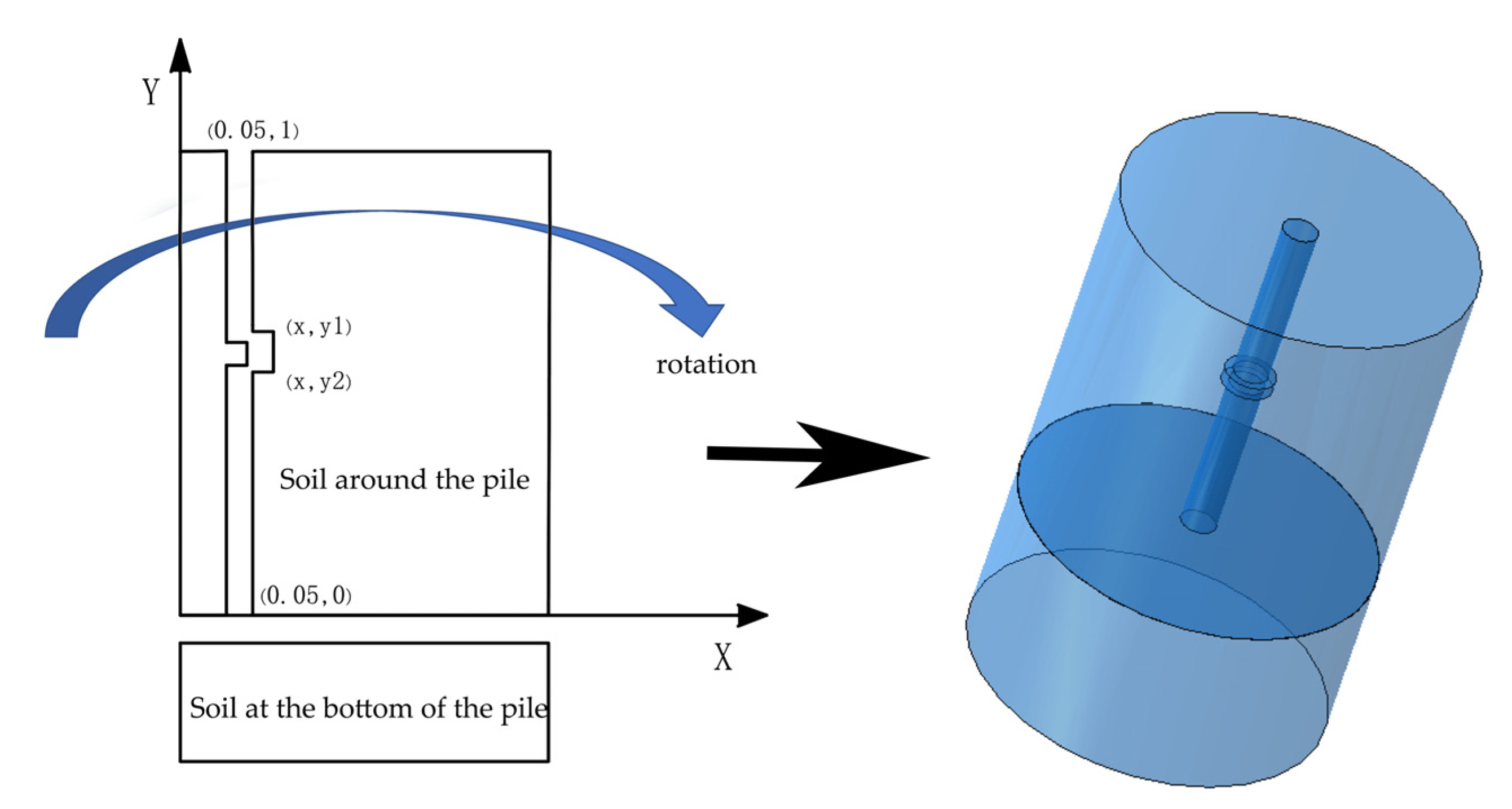
2.3.2. Specific Modeling Method

According to the basic parameters and theories in the previous section, the finite element models for five types of defective piles were established in this study. The model consists of three parts: the soil around the pile, the soil under the pile, and the concrete pile, as shown in Figure 4. Instantaneous sinusoidal stress is applied to the top of the pile to simulate the process of applying excitation during LSPIT detection; the form of applying stress can be shown in Formula (9) [39]. The sensor was replaced by the history output in Abaqus, and the sensor is normally placed at 2/3 of the radius of the pile top during the LSPIT detection [27], so a point was selected at 2/3 of the radius of the pile top to output the speed signal of the point during the test process to simulate the function of the sensor.
p ( t ) = p 0 sin ( π t T d ) 0 t T d
For neck defects and bulge imperfections, the main reason for the LSPIT signal change was the impedance change caused by the increase or decrease in pile diameter, which was directly related to the shape of the pile. Therefore, in this study, in the finite element model, the diameter of the defected part was increased and reduced in a certain proportion to simulate the neck defect and bulge imperfection defect, as shown in Figure 5.
For weak concrete piles, the main reason for the change of the test signal was that when the wave propagates in an uneven medium, due to the change of the elastic modulus of the material, the impedance changes abruptly, and some waves are reflected to the top of the pile at the defect, resulting in the change of LSPIT signal. The weak concrete pile is generated by reducing the elastic modulus of the material at the defect site, as shown in Figure 5.
Five kinds of piles were numerically simulated by the parameters shown in Table 1, and the results are shown in Figure 6.
For crack piles, the existence of cracks will hinder the downward propagation of waves, which will be reflected by the LSPIT signal collected at the pile top. The crack is modeled over the special seam crack ABAQUS function. In this case, the crack surfaces are separated with zero distance. The interaction between the surfaces is implemented as a kinematic contact assignment to prevent penetration [43,44].
When the broken defect occurs, this study assumes that the pile body was completely broken into two parts. At this time, the pile was not a continuous whole, and the change of the elastic modulus of the material around the defect was very small, which hardly affects the LSPIT signal. The real reason for the change of the signal was the geometric shape of the pile and the interaction between the broken piles [14]. Therefore, under the premise of this assumption, when the pile was broken, the pile was broken into two independent parts. During the modeling, the contact form between the two parts of the pile was set to hard contact to simulate this defect form [45].
The black point represents the time point when the wave begins to enter from the top of the pile, the red point represents the time point when the wave is reflected from the bottom of the pile to the top of the pile, and the red frame line represents the reflection of the wave at the defect site. By analyzing the characteristics of the wireframe part, the type of defect can be obtained.
For the neck defect pile, the red time point is 0.000651376 s and the black time point is 0.000105197. It can be concluded that the time of wave propagation from the top of the pile to the bottom of the pile and reflection back to the top of the pile is 0.00055 s. Through the formula c = E / ρ , the propagation velocity of the wave in C30 concrete is 3464 m/s. The pile length can be calculated to be 3464 × 0.00055/2 = 0.952 m. The difference from the actual value of 1 m is less than 0.05 m, and the accuracy of the numerical simulation meets the expectation.
For the bulge imperfections pile, the red point time is 0.000675, the black point time is 0.00010538, and the total time length of wave propagation is 0.00056962. The calculated pile length is 0.987 m, which meets the expectation.
For weak concrete, the red point time is 0.00066622 s, the black point time is 0.0005582 s, and the wave propagation time is 0.00055815 s. The calculated pile length is 0.967 m, which meets the expectation.
For the crack pile, the red point time is 0.000633, the black point time is 0.000101, and the total time length of wave propagation is 0.000532. The calculated pile length is 0.921 m, which meets the expectation.
The broken pile has broken into two parts and is no longer a continuous whole, the wave cannot be transmitted to the bottom of the pile, and the wave is reflected to the top of the pile after it is transmitted to the broken part. Therefore, there are multiple peaks similar to the reflection of the bottom of the pile in the time domain diagram. This feature can be easily discovered by inspectors and determine the type of defect.

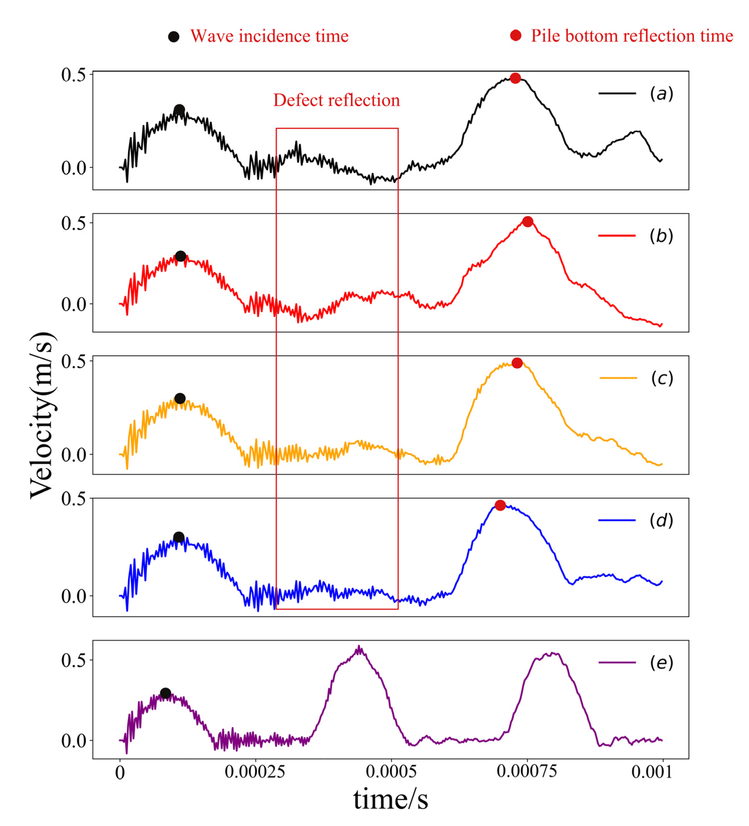
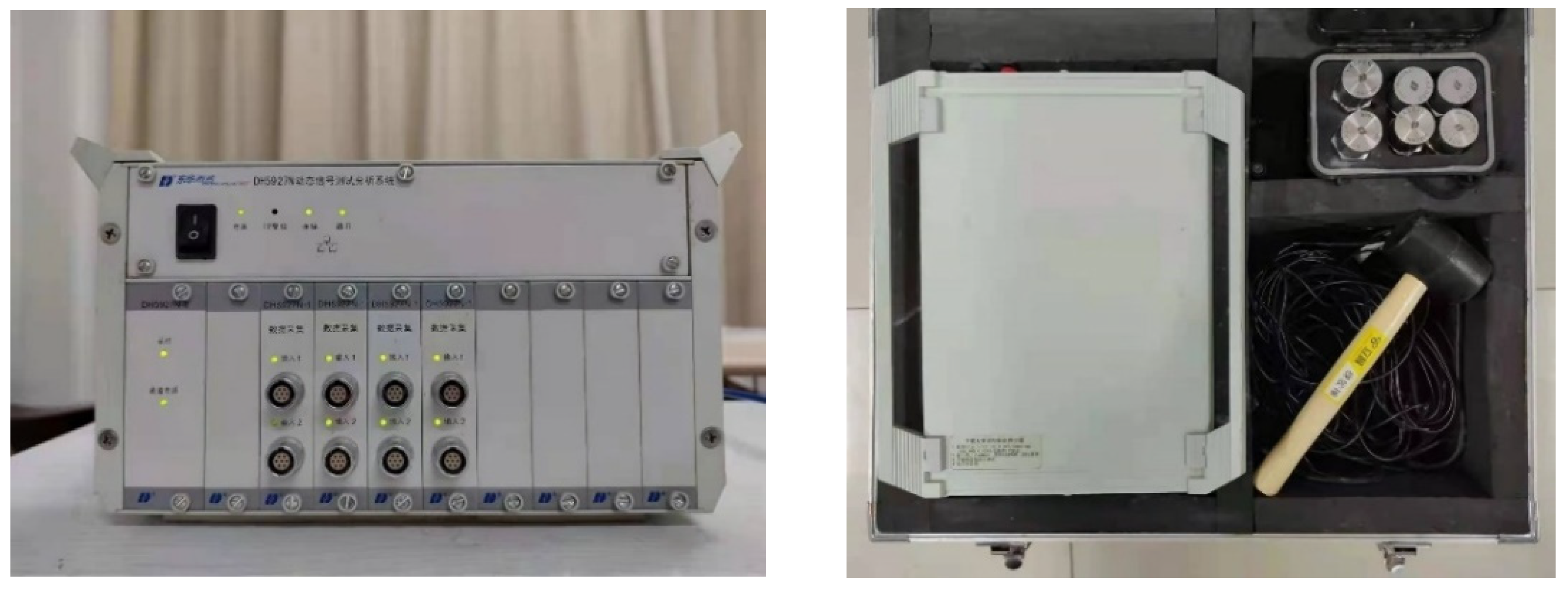
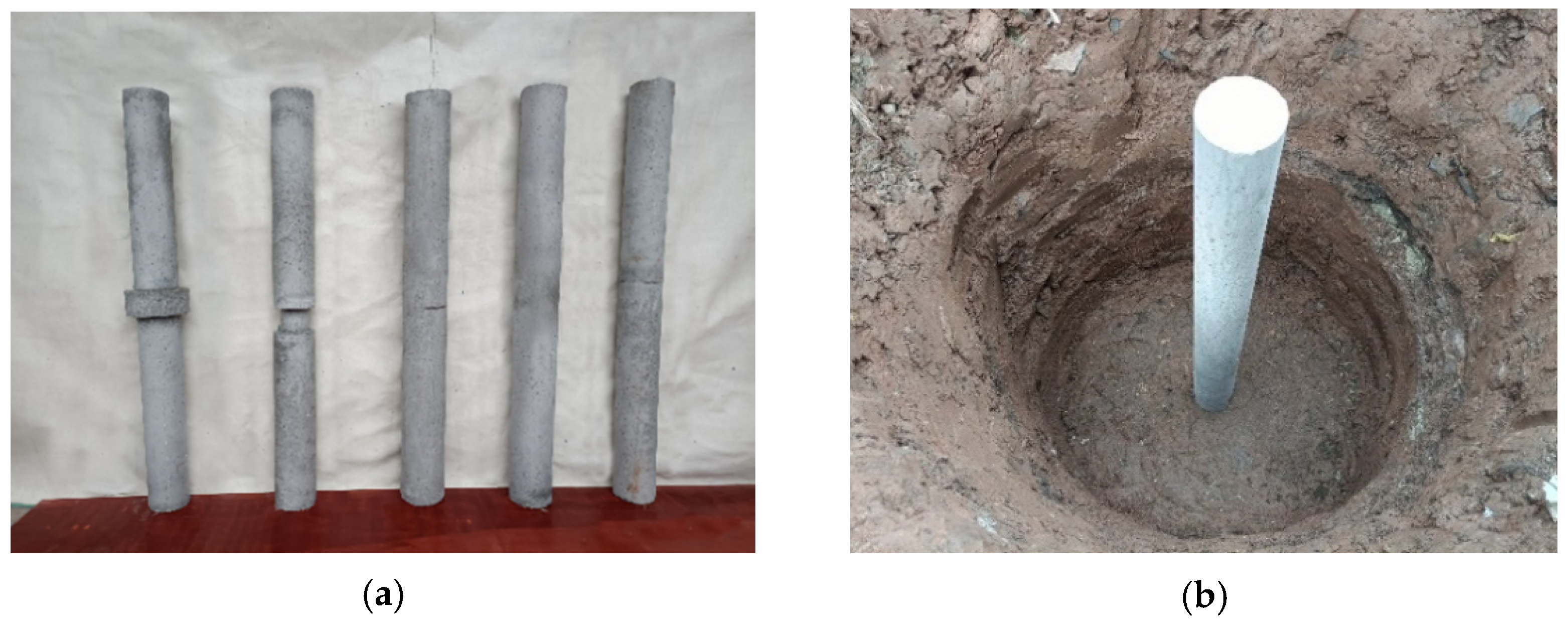
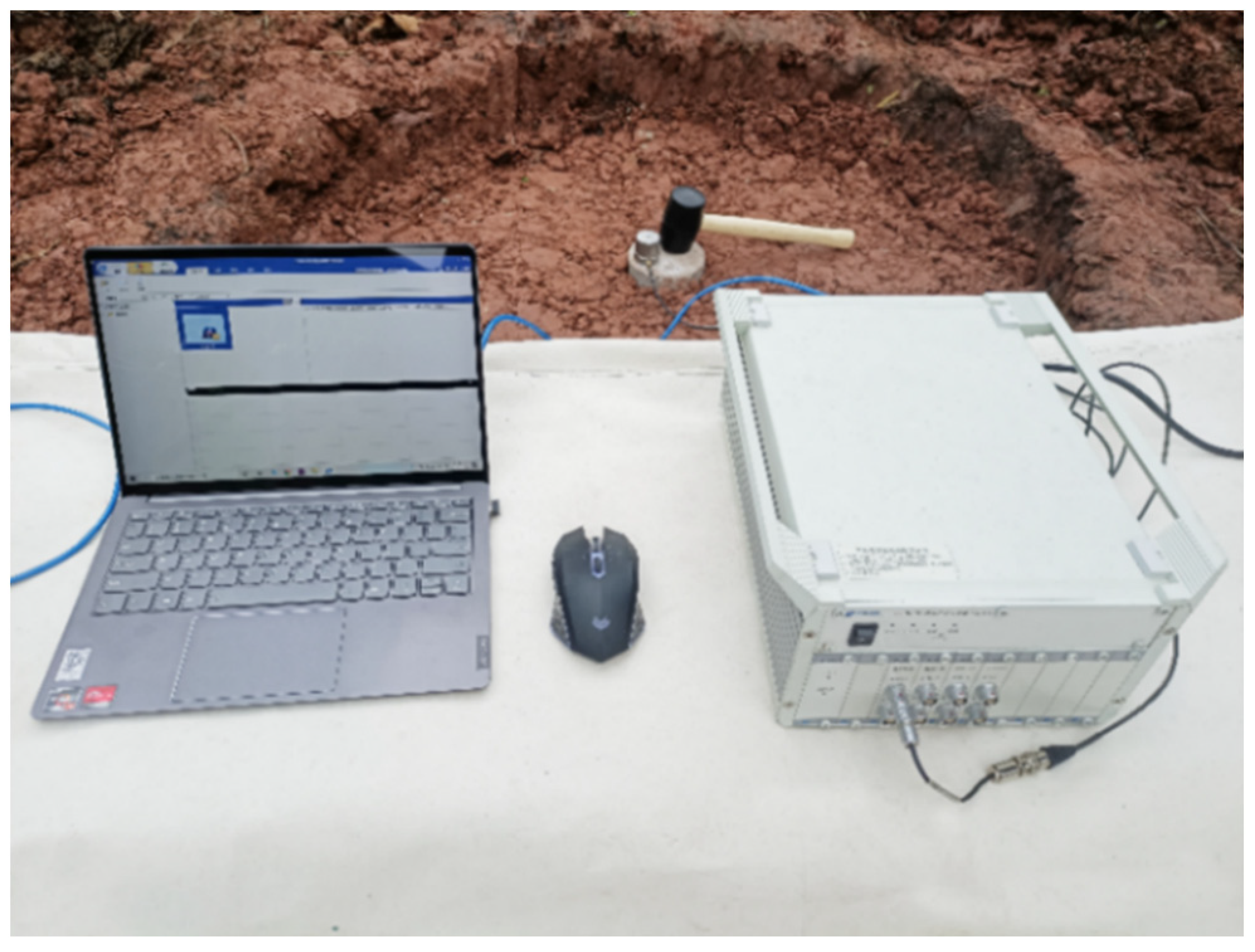
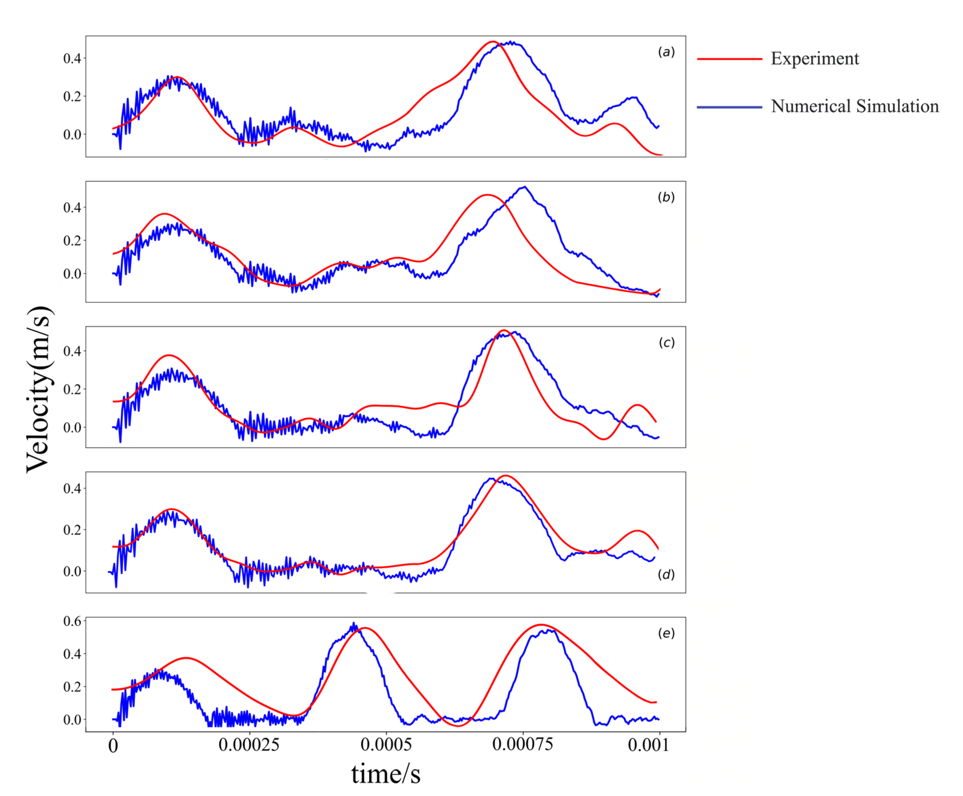
2.4. Experimental Validation

To verify the results of this paper, the experiment was used to verify the model in this paper. C30 concrete was used as the normal pile material, clay was used as the soil around the pile and the soil at the bottom of the pile, and C15 concrete was used as the weak concrete part of the weak concrete pile. Five piles (bulge imperfection, neck defect, cracks, weak concrete, broken) were made. The crack pile and broken pile are generated by cutting the pile body. The weak concrete pile was generated by pouring low-grade concrete at the defect position, and the defect position is set in the middle of the pile body. The specific parameters of the model are shown in Table 2.
The equipment required for the experiment includes a DH5927N dynamic signal tester (Donghua Testing Technology Co., Ltd., Jingjiang, China), rubber hammer, acceleration sensor, and transmission data line, as shown in Figure 7. DH5927N dynamic signal test instrument is mainly used for dynamic signal analysis and acquisition. The acceleration sensor is used to collect the vibration signal of the pile, and the rubber hammer is used to generate excitation. The sensitivity of the sensor is 1006 mv/g. The sensor is connected with the first channel of DH5927N by using the data transmission line, and the first channel is cleared. The measurement range of the channel is set to 0–0.099, the sampling frequency is set to 200,000 Hz, and the sampling time is set to 0.00012 s.
After 28 days of maintenance of the specimen, the pit with a depth of 1 m and a diameter of 1 m was excavated at the experimental site. The pile was placed at the center of the pit and backfilled with undisturbed uniform clay. Layered compaction of pile and soil ensured the same degree of compaction in each layer of soil around the pile as shown in Figure 8. (COOK obtained by analyzing the experimental data of London clay that when the radius of soil around the pile was about 10 R, the shear displacement was almost negligible. For practical engineering, when the radius of soil around the pile was set to 5–6 R, it could meet the requirements of practical engineering. Therefore, in this experiment, when the radius of soil around the pile was set to 10 times that of the pile, it could meet the requirements of practical engineering [42]).
After the piles were landfilled, the LSPIT signals were collected. A total of 50 data were collected for each type of defective pile, and a total of 50 × 5 = 250 data were collected for five types of piles. The collected acceleration signals were integrated to obtain the velocity signal, and then the next set of data processing was carried out. The experimental process is shown in Figure 9.
Draw the data in Figure 6 and the experimental data into one figure, Through the data comparison, it can be found that there is a high matching between the experimental data and the simulation data. The reflection of the pile bottom is visible. The reflection signal of the defect location can better reflect the occurrence of the defect. The experiment proves the effectiveness of the numerical simulation. As shown in Figure 10.

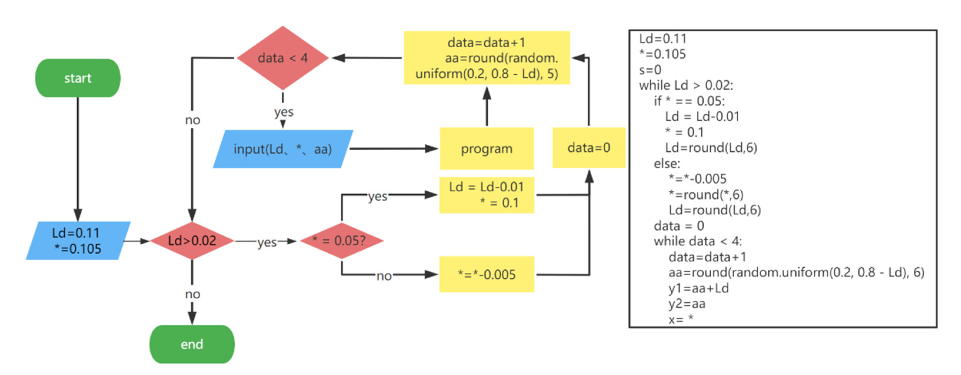
2.5. Batch Modeling Using Python Scripts

To obtain a large amount of defective pile data and establish a reasonable defective pile foundation data set, this paper used Python language to write an ABAQUS script that generates defective pile foundation data. The operation of the ABAQUS software is based on the Python language, so it can be directly written by Python files to control the generation of the model [38]. The steps of model generation are (1) sketch parts; (2) properties; (3) assembly; (4) analysis step; (5) interaction; (6) load; (7) grid; (8) job; (9) post-processing. The main function of scripts is to control the size of defects. In this study, the parts that need to be revised are (1), (9), and (2) in each modeling; other steps do not need to change. By controlling the corresponding variables of those parts to achieve the purpose of generating different defects.
Taking the establishment logic of the bulge imperfection pile model as an example, as shown in Figure 11, the Python loop was used to control variables to generate finite element models of defective piles with different degrees. The variables are the radius of the defect, length of defect, and location of the defect. The script contains two loops; the main loop determines the radius * and length L d of the defect, and the second loop determines the location aa of the defect. The end of each loop will pass parameters to the “program” for generation and calculation of the model.
The finite element model was generated by the rotation command in Abaqus, as shown in Figure 12, and the “program” in the script controls the calculation of the model and the generation of other invariants, such as the application of the excitation force, the assignment of the material, the setting of the analysis step, the meshing, the assembly of the components, the setting of the interaction, the output, the processing of the data, etc. Those parts do not affect the degree of the defect and do not need to be set to variables (The logic of the other scripts is similar to the bulge imperfection pile and is explained in turn below. The modeling parameters are shown in Table 3).
For neck defects and bulge imperfections, in the main loop, 10 * corresponds to 10 L d , and 100 sets of parameters were generated in turn. In the second loop, each set of parameters corresponds to 4 aa (defect location); a total of 400 sets of data are generated and input into the “program” in turn.
As shown in Figure 13, for weak concrete piles in the main loop, 10 weak material data are generated according to elastic modulus from small to large; each type of material corresponds to 10 L d , and 100 sets of parameters are generated. In the second loop, 4 aa corresponds to 100 sets of parameters in turn. which makes the amount of defect data reach 10 × 10 × 4 = 400.
For cracked piles, the range of cracks, the angle of cracks, and the location of cracks were set as variables. The crack was modeled over the special seam crack ABAQUS® function, which determines the location and range of cracks by script parameters [43]. In the main loop, each r corresponds to each a and generated 100 sets of parameters. In the second loop, 4 aa corresponds to each parameter generated in the main loop. A total of 10 × 10 × 4 = 400 data were generated. The modeling idea was shown in Figure 13.
For the modeling of broken piles, the pile was set as two parts, and the interaction between the upper and lower parts of the pile was set to hard touching to simulate the occurrence of a break [45]. The location of the broken part was seated as a variable to generate 400 broken pile data.

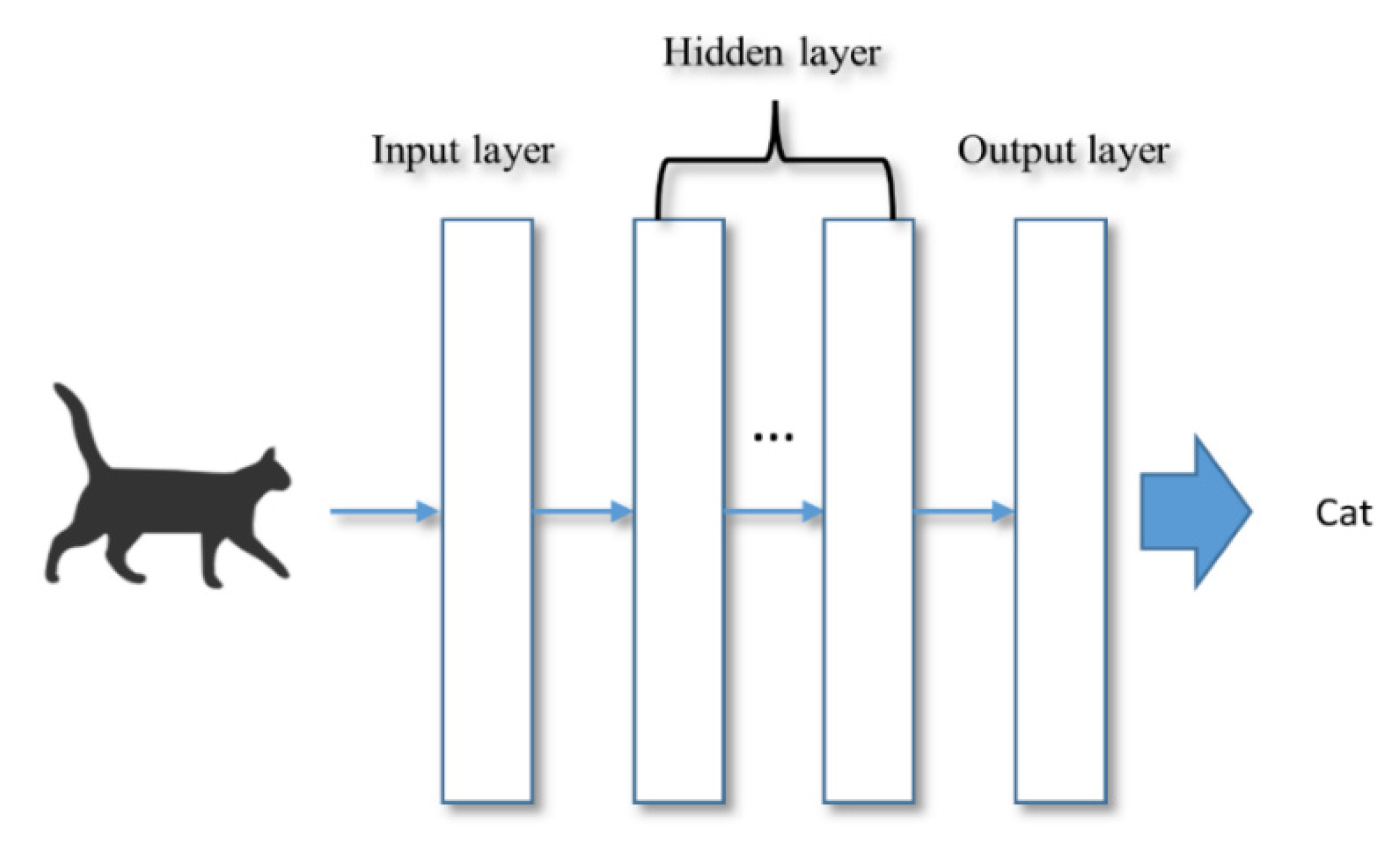
2.6. Convolution Neural Network

CNNs are deep learning frameworks based on the working principle of animal neurons and are widely used in image recognition and classification. Their core idea is to imitate biological vision through feature mapping, weight sharing, local connection, and pooling operation. Its special network structure can transform the large dimensions image into an array and input it into neural networks. The structure of a CNN is layered (Figure 14); a basic CNN consists of the input layer, convolution layer, pooling layer, fully connected layer, and output layer [44]. The convolution layer and pooling layer are mainly used to reduce feature dimension, compress the number of data and parameters, reduce overfitting, and improve the fault tolerance of the model. The full connection layer is used to classify images and serve as a classifier. The way to implement convolution operations is the following Formula (10).
s ( t ) = f ( x ) w ( t x ) d x
Functions f ( x ) and w ( t     x ) are convolution objects “*” representing convolution calculations. After the above operation, the feature map of data can be obtained.
Details of the CNN architecture are presented in Table 4 and Figure 15. The RMSprop algorithm [46] was used as the optimizer and ReLU [47] was used as the activation function across the network. This optimizer and the activation function were chosen because they could get higher accuracy and faster convergence speed and were suitable for processing non-stationary signals. In this study—to improve recognition accuracy, reduce the calculation parameters, and avoid over-fitting—three convolutional layers, two pooling layers, and one dropout layer are used. The learning rate was set as 0.001 and the network was trained for 200 epochs with a batch size of 32.

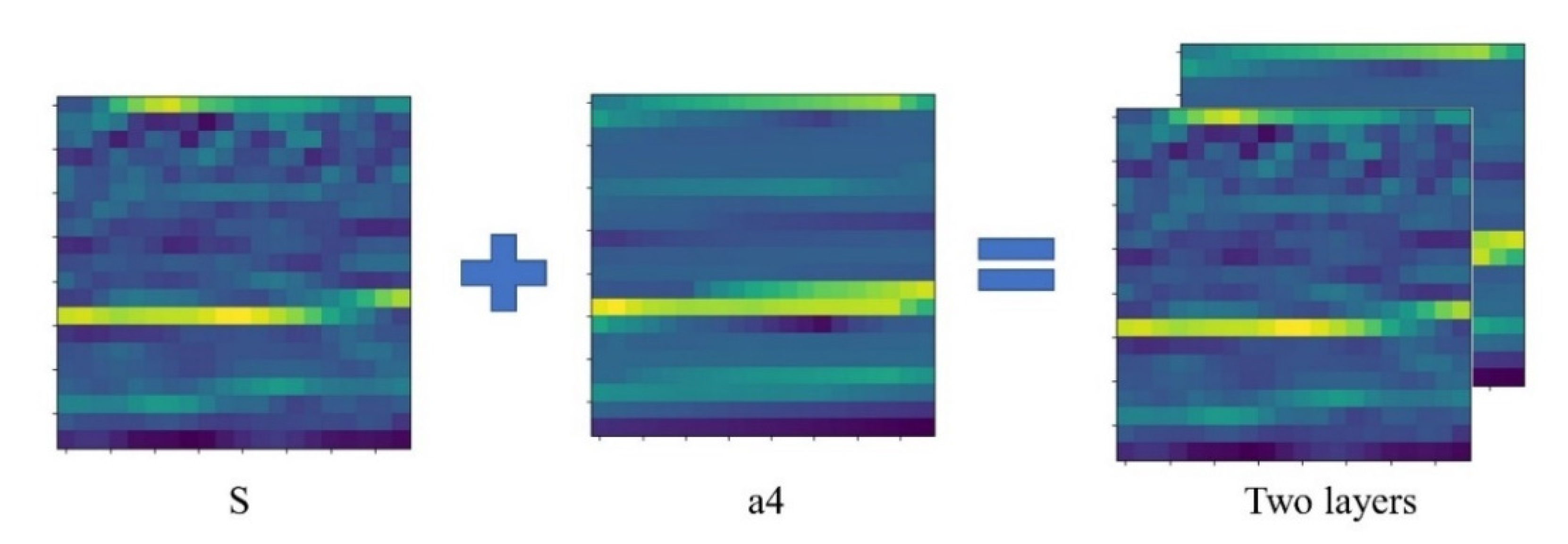
2.7. Data Enhancement and WPT
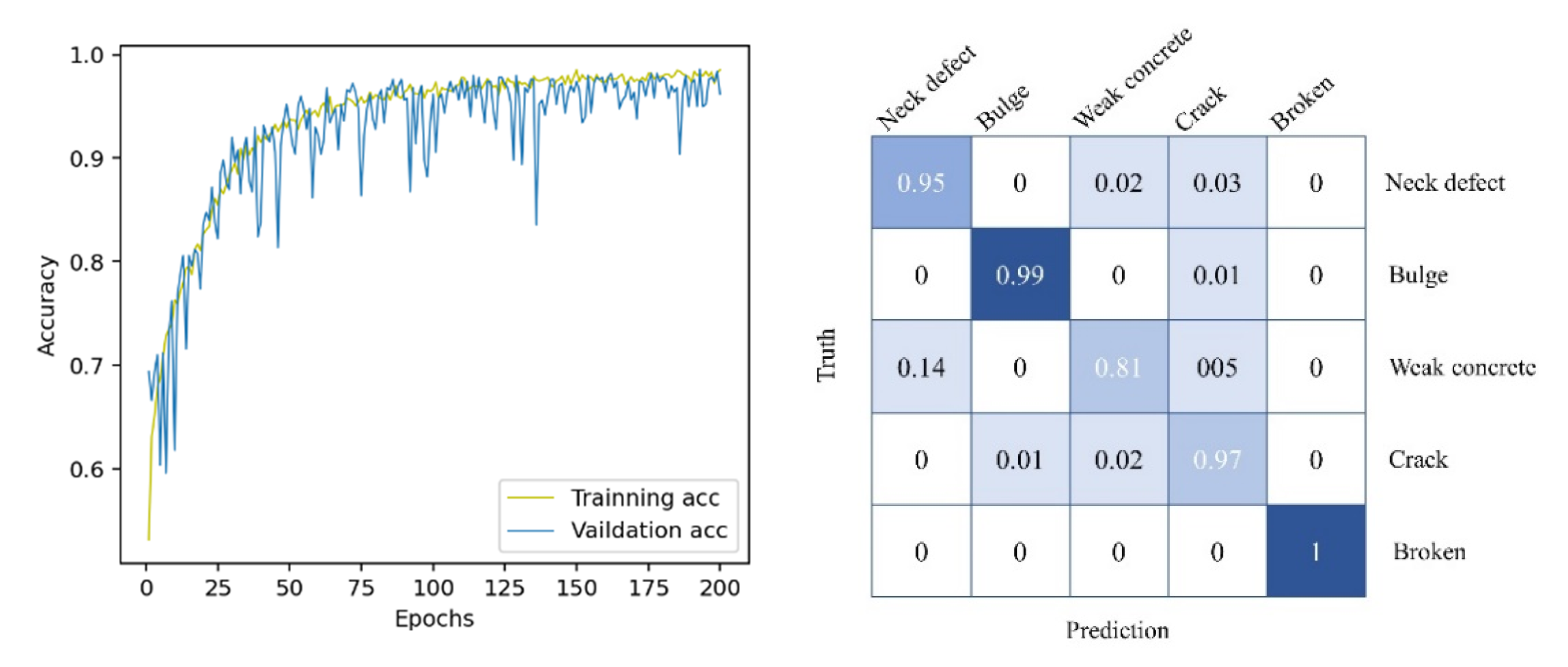
To obtain higher recognition accuracy, it was necessary to denoise and enhance the original data. In this study, the original data were decomposed and reconstructed using the WPT technique, and to prevent the data from losing too much information after WPT, this study fused the original data with the data reconstructed by wavelet to generate multidimensional feature indicators to obtain more accurate feature metrics.
To get a better denoising effect, this paper chooses the wavelet basis function db2 similar to the original data waveform as the basis function of WPT, and its waveform is similar to the transient vibration of the original data. The level of decomposition is equally important to the success of noise reduction. In general, too many decomposition layers lead to a severe loss of signal information, a decrease in SNR, and an increase of computational complexity. Conversely, if the number of decomposition layers is too small, the noise reduction effect is limited, and the improvement of the signal-to-noise ratio is also limited [48].
LSPIT data were processed by wavelet transform to obtain the high-frequency signal di and low-frequency signal ai of each level, as shown in Figure 16. It can be seen from Figure 16 that as the number of decomposition layers increases, the noisy data become smaller and smaller. The noise in the signal was too small to distinguish until it was decomposed to level 4. At the same time, the signal of the fourth level was the same as the main waveform in the original signal. When the number of decomposition levels exceeds four, the gap with the original signal becomes large.
This paper used the advantages of the CNN processing multilayer data to enhance the data. Through the principle of wavelet decomposition, it is found that although wavelet decomposition can remove the high-frequency noise in the signal, the high-frequency data still contains some important information. In this research, there is still a certain spatial relationship between the original signal and the signal of the fourth layer of the wavelet decomposition. To prevent the data from losing too much information after wavelet reconstruction, the single-layer 20 × 20 original data S and the single-layer 20 × 20 wavelet decomposition fourth level data a4 were superimposed and normalized (divide each value into the data by the number with the largest absolute value in the data so that each value in the data is between 1 and −1). After the original data were randomly disrupted, the pywt wavelet packet library in Python was used to directly decompose and reconstruct the original data, and the NumPy library was used to reconstruct the structure of the data to generate the data form of 20 × 20 × 2. Then, two layers of 20 × 20 data were generated and fed into the neural network for training, as shown in Figure 17. For training, 25% of the data was set as the validation set, 75% was set as the training set; the learning rate was set to 0.001, training for 200 epochs, and batch size was 32.

3. Result

The result of the training is shown in Figure 18. The accuracy rate obtained on the verification set is about 94.4%. Through the confusion matrix and the accuracy rate map, the training result can be seen. The accuracy rate graph shows the increase of the accuracy rate during the training of 200 epochs, and the confusion matrix shows the recognition accuracy rate and Specific misidentification situation of five types of defects.
For the neck defect data set, 95% of the data were correctly identified, 2% of the data was identified as a weak concrete defect, and 3% of the data were identified as a crack defect.
For the bulge imperfection data set, 99% of the data were correctly identified; 1% of the data were identified as cracks.
For the weak concrete data set, only 81% of the data were correctly identified, and 14% of the data were identified as a neck defect.
For crack defects, 97% of the data were correctly identified, 1% of the data were identified as bugle defects, and 2% of the data were identified as weak concrete.
For broken defects, 100% of the data were correctly identified.

4. Conclusions

The results of this study were based on a large number of numerical simulations. Although good results were obtained there was no large-scale experimental data validation and the experimental scale of this study was small. In the future, research using large-scale data sets will produce more convincing results.
In this paper, five types of piles with different defect degrees were simulated and verified by experiments. The finite element software and Python scripts are used to simulate the different defect degrees of five common types of defective piles. The LSPIT signals of five types of defective piles were measured, and the CNN model was established. The LSPIT signals were used for supervised training. Therefore, in this study, wavelet packet analysis is first used to decompose the original signal into four layers. After the fourth layer signal of the low-frequency part is reconstructed, the original signal and the fourth layer signal of the WPT are folded and overlapped to obtain a two-dimensional array of 20 × 20 × 2. The data set, which contained 2000 data, was randomly divided into a 1500-data training set and a 500-data test set. Finally, 472 items were correctly classified on the test set containing 500 data. The conclusions are as follows:
(1)
The application of LSPIT is affected by many complex situations, such as the influence of environmental noise on low-strain data and the influence of rebound waves superimposed on each other in concrete piles, but these influences will not destroy the information contained in low-strain data. Therefore, signal processing by computer technology can help to extract the characteristic indexes of the signal and eliminate the influence of complex conditions on the signal.
(2)
After feature extraction and signal structure reconstruction of the signal, a CNN can be used as an auxiliary tool for defect identification of concrete pile defects by the low-strain reflection wave method.
(3)
The complex noise in the original signal has a negative impact on the performance of the CNN classifier. The performance and robustness of the CNN classifier were increased by WPT and data enhancement. Using WPT and data enhancement can improve the accuracy of signal recognition compared with using only velocity signals as a defect index.

Author Contributions

Conceptualization, C.-S.W.; Data curation, J.-Q.Z.; Formal analysis, C.-S.W., L.-L.Q., and D.-B.Z.; Investigation, J.-Q.Z. and L.-L.Q.; Methodology, C.-S.W.; Project administration, D.-B.Z.; Resources, D.-B.Z.; Software, J.-Q.Z.; Supervision, D.-B.Z.; Validation, J.-Q.Z.; Writing—original draft, C.-S.W.; Writing—review & editing, L.-L.Q. All authors have read and agreed to the published version of the manuscript.

Funding

This research was supported by the Fund of the National–Local Joint Engineering Laboratory for Road Engineering and Disaster Prevention and Mitigation Technology in Mountainous Areas (No. 2018Road002) and was also supported by the Open Fund Project of Chongqing Jiaotong University’s Key Laboratory of Mountainous Highway and Water Transportation Geological Disaster Reduction (kfxm 2018-05).

Institutional Review Board Statement

Not applicable.

Informed Consent Statement

Not applicable.

Data Availability Statement

Not applicable.

Conflicts of Interest

The authors declare no conflict of interest.

References

  1. Rausche, F. Non-destructive evaluation of deep foundations. In Proceedings of the 5th International Conference on Case Histories in Geotechnical Engineering, New York, NY, USA, 13–17 April 2004; pp. 1–9. [Google Scholar]
  2. Chow, Y.K.; Phoon, K.K.; Chow, W.F. Low strain integrity testing of piles: Three-dimensional effects. J. Geotech. Geoenvironmental Eng. 2003, 129, 1057–1062. [Google Scholar] [CrossRef]
  3. Luo, W.; Chen, F.; Hu, J. Improvement of Low Strain Pile Integrity Test. In Proceedings of the ASEE (American Society of Engineering Education) Conference, Boston, MA, USA, 7–8 May 2010; pp. 583–589. Available online: https://monolith.asee.org/documents/zones/zone1/2008/student/ASEE12008_0082_paper.pdf (accessed on 11 April 2022).
  4. Liu, W.; Tian, S. Classification of pile integrity based on convolutional neural network. J. Nanchang Univ. (Eng. Ed. ) 2021, 43, 263–268. [Google Scholar] [CrossRef]
  5. Bao, L.S.; Ye, X.F.; Li, Q.; Wang, H. Research on the application of neural network based on genetic algorithm in pile foundation detection. Highw. Transp. Technol. (Appl. Technol. Version) 2017, 13, 228–231. [Google Scholar]
  6. Tam, C.M.; Tong, T.K.L.; Lau, T.C.T. Diagnosis of prestressed concrete pile defects using probabilistic neural networks. Eng. Struct. 2004, 26, 1155–1162. [Google Scholar] [CrossRef]
  7. Cui, D.M.; Yan, W.; Wang, X.Q. Towards intelligent interpretation of low strain pile integrity testing results using machine learning techniques. Sensors 2017, 17, 2443. [Google Scholar] [CrossRef] [Green Version]
  8. Yan, T.N.; Wang, S.; Li, S.J. The application of artificial neural network method in pile foundation detection. Geol. Sci. Technol. Inf. 1999, (Suppl. S1), 38–41. [Google Scholar]
  9. Cai, Q.Y.; Lin, J.H. Diagnosis of pile defects based on wavelet analysis and neural network. Vib. Impact 2002, 3, 13–16. [Google Scholar] [CrossRef]
  10. Cai, Q.Y. Diagnosis of Pile Defects Based on Wavelet Analysis and Neural Network. Master’s Thesis, Huaqiao University, Quanzhou, China, 2001. [Google Scholar]
  11. Wang, C.H.; Zhang, W. Neural network model for pile integrity identification based on reflection wave method. Geotech. Mech. 2003, 6, 952–956. [Google Scholar] [CrossRef]
  12. Liu, M.G.; Yue, X.H.; Yang, Y.B.; Li, Q. Intelligent identification of pile defects based on Sym wavelet and BP neural network. J. Rock Mech. Eng. 2007, 192 (Suppl. S1), 3484–3488. [Google Scholar]
  13. Zhang, G.; Jiang, X.L.; Liu, Z.J. Pile defect intelligent identification based on wavelet analysis and neural networks. In Applied Mechanics and Materials; Trans Tech Publications Ltd.: Frienbach, Switzerland, 2014; Volume 608–609, pp. 899–902. [Google Scholar] [CrossRef]
  14. Protopapadakis, E.; Schauer, M.; Pierri, E. A genetically optimized neural classifier applied to numerical pile integrity tests considering concrete piles. Comput. Struct. 2016, 162, 68–79. [Google Scholar] [CrossRef]
  15. Kang, W.; Zhao, Y.; Liu, L. Pile defect identification based on multi-higher order moment feature. J. GeoEng. 2018, 13, 69–77. [Google Scholar]
  16. Vu, G.; Timothy, J.J.; Singh, D.S. Numerical simulation-based damage identification in concrete. Modelling 2021, 2, 355–369. [Google Scholar] [CrossRef]
  17. Xie, Y.; Xiao, Y.; Liu, X. Time-frequency distribution map-based convolutional neural network (CNN) model for underwater pipeline leakage detection using acoustic signals. Sensors 2020, 20, 5040. [Google Scholar] [CrossRef]
  18. Zhuo, D.B.; Cao, H. Joint damage identification based on wavelet time-frequency diagram and lightweight convolutional neural network. Eng. Mech. 2021, 38, 228–238. [Google Scholar]
  19. Ritto, T.G.; Rochinha, F.A. Digital twin, physics-based model, and machine learning applied to damage detection in structures. Mech. Syst. Signal Processing 2021, 155, 107614. [Google Scholar] [CrossRef]
  20. Karvelis, P.; Georgoulas, G.; Kappatos, V. Deep machine learning for structural health monitoring on ship hulls using acoustic emission method. Ships Offshore Struct. 2021, 16, 440–448. [Google Scholar] [CrossRef]
  21. Rautela, M.; Senthilnath, J.; Moll, J. Combined two-level damage identification strategy using ultrasonic guided waves and physical knowledge assisted machine learning. Ultrasonics 2021, 115, 106451. [Google Scholar] [CrossRef]
  22. Perry, B.J.; Guo, Y. Atadero, R. Streamlined bridge inspection system utilizing unmanned aerial vehicles (UAVs) and machine learning. Measurement 2020, 164, 108048. [Google Scholar] [CrossRef]
  23. Li, Z.; Li, D.; Chen, Y. Deep learning-based guided wave method for semi-grouting sleeve detection. J. Build. Eng. 2022, 46, 103739. [Google Scholar] [CrossRef]
  24. Rausche, F.; Moses, F.; Goble, G.G. Soil resistance predictions from pile dynamics. J. Soil Mech. Found. Div. 1972, 98, 917–937. [Google Scholar] [CrossRef]
  25. Kim, H.J.; Mission, J.L.; Dinoy, P.R. Guidelines for impact echo test signal interpretation based on wavelet packet transform for the detection of pile defects. Appl. Sci. 2020, 10, 2633. [Google Scholar] [CrossRef] [Green Version]
  26. Smith, E.A.L. Pile-driving analysis by the wave equation. J. Soil Mech. Found. Div. 1960, 86, 35–61. [Google Scholar] [CrossRef]
  27. ASTM D5882-07; Standard Test Method for Low Strain Impact Integrity Testing of Deep Foundations. ASTM International: West Conshohocken, PA, USA, 2007.
  28. Dai, Y.W. Reliability Method for Damage Identification of Solid Concrete Piles Based on Low Strain Reflection Wave Method. Ph.D. Thesis, South China University of Technology, Guangzhou, China, 2018. [Google Scholar]
  29. Yuan, Q.; Zhou, W.; Zhang, L. Epileptic seizure detection based on imbalanced classification and wavelet packet transform. Seizure 2017, 50, 99–108. [Google Scholar] [CrossRef] [PubMed]
  30. Han, J.G.; Ren, W.X.; Sun, Z.S. Wavelet packet based damage identification of beam structures. Int. J. Solids Struct. 2005, 42, 6610–6627. [Google Scholar] [CrossRef] [Green Version]
  31. Bettayeb, F.; Haciane, S.; Aoudia, S. Improving the time resolution and signal noise ratio of ultrasonic testing of welds by the wavelet packet. NDT E Int. 2005, 38, 478–484. [Google Scholar] [CrossRef]
  32. Yen, G.G.; Lin, K.C. Wavelet packet feature extraction for vibration monitoring. IEEE Trans. Ind. Electron. 2000, 47, 650–667. [Google Scholar] [CrossRef] [Green Version]
  33. Schauer, M.; Langer, S. Numerical simulations of pile integrity tests using a coupled FEM SBFEM approach. PAMM 2012, 12, 547–548. [Google Scholar] [CrossRef]
  34. Huang, Y.H.; Ni, S.H.; Lo, K.F. Assessment of identifiable defect size in a drilled shaft using sonic echo method: Numerical simulation. Comput. Geotech. 2010, 37, 757–768. [Google Scholar] [CrossRef]
  35. Doebling, S.W.; Farrar, C.R.; Prime, M.B. Damage Identification and Health Monitoring of Structural and Mechanical Systems from Changes in Their Vibration Characteristics: A Literature Review. Available online: https://www.osti.gov/biblio/249299 (accessed on 11 April 2022).
  36. Liao, S. Nondestructive Testing of Piles. Ph.D. Thesis, The University of Texas at Austin, Austin, TX, USA, 1994. [Google Scholar]
  37. Kim, H.J.; Mission, J.L.C.; Park, I.S. Analysis of static axial load capacity of single piles and large diameter shafts using nonlinear load transfer curves. KSCE J. Civ. Eng. 2007, 11, 285–292. [Google Scholar] [CrossRef]
  38. ABAQUS User’s Manual-Version 6.7; SIMULIA Dassault Systemes: Vélizy-Villacoublay, France, 2007.
  39. Li, J.B. Numerical Simulation and Application of Elastic Wave Method for Bridge Pile Detection in South Sichuan Intercity Railway. Master’s Thesis, Southwest Jiaotong University, Chengdu, China, 2020. [Google Scholar]
  40. Ni, S.H.; Lo, K.F.; Lehmann, L. Time–frequency analyses of pile-integrity testing using wavelet transform. Comput. Geotech. 2008, 35, 600–607. [Google Scholar] [CrossRef]
  41. Lu, Z.T.; Wang, Z.L.; Liu, D.J. Study on low-strain integrity testing of pipe-pile using the elastodynamic finite integration technique. Int. J. Numer. Anal. Methods Geomech. 2013, 37, 536–550. [Google Scholar] [CrossRef]
  42. Cooke, R.W.; Price, G.; Tarr, K. Jacked piles in London clay: Interaction and group behaviour under working conditions. Geotechnique 1980, 30, 97–136. [Google Scholar] [CrossRef]
  43. Gschossmann, S.; Oberascher, T.; Schagerl, M. Quantification of subsurface cracks in a thin aluminium beam by the use of nonlinear guided wave theory–a numerical and model-based approach. In Proceedings of the 9th EWSHM, Manchester, UK, 10–13 July 2018; pp. 10–13. [Google Scholar]
  44. Sun, Y.; Ma, S.; Sun, S. Partial discharge pattern recognition of transformers based on mobilenets convolutional neural network. Appl. Sci. 2021, 11, 6984. [Google Scholar] [CrossRef]
  45. Cao, K. Research on pile defects based on low strain reflection wave method. Master’s Thesis, Hebei University, Baoding, China, 2018. [Google Scholar]
  46. Dozat, T. Incorporating Nesterov Momentum into Adam. Available online: https://openreview.net/pdf?id=OM0jvwB8jIp57ZJjtNEZ (accessed on 11 April 2022).
  47. Nair, V.; Hinton, G.E. Rectified linear units improve restricted boltzmann machines. In Proceedings of the ICML, Haifa, Israel, 21–24 June 2010. [Google Scholar]
  48. Zhang, B.; Muradov, K.; Dada, A. Principal component analysis-assisted selection of optimal denoising method for oil well transient data. J. Pet. Explor. Prod. 2021, 11, 509–530. [Google Scholar] [CrossRef]
Figure 1. Low-strain pile integrity test.
Buildings 12 00664 g001
Figure 2. Tree structures of wavelet packet transform (A represents low frequency, D represents high frequency, and the number represents the number of layers of decomposition).
Buildings 12 00664 g002
Figure 3. Types of simulated pile foundation ((a) neck defect; (b) bulge imperfection; (c) weak concrete; (d) crack; (e) broken pile)).
Buildings 12 00664 g003
Figure 4. Finite element mesh of pile and soil.
Buildings 12 00664 g004
Figure 5. The finite element model of five kinds of piles.
Buildings 12 00664 g005
Figure 6. Numerical simulation data. ((a) neck defect; (b) bulge imperfection; (c) weak concrete; (d) crack; (e) broken pile).
Buildings 12 00664 g006
Figure 7. Experimental apparatus.
Buildings 12 00664 g007
Figure 8. (a) Experimental piles (bulge imperfection; neck defect; crack; weak concrete; broken); (b) Placement of experimental pile.
Buildings 12 00664 g008
Figure 9. Process of the experiment.
Buildings 12 00664 g009
Figure 10. Experimental data ((a) neck defect; (b) bulge imperfection; (c) weak concrete; (d) crack; (e) broken pile).
Buildings 12 00664 g010
Figure 11. Basic logic of scripts.
Buildings 12 00664 g011
Figure 12. Principle of model generation.( X represents the radial direction of the pile, Y represents the longitudinal direction of the pile).
Buildings 12 00664 g012
Figure 13. Parameters of five kinds of defects (pile (a) and pile (b) have three variables: defect location aa, defect length, and defect radius *. The variables of pile (c) are defect location aa, defect length, and the material properties of the defective part. The variable of pile (e) is the position of defect aa. The variables of pile (d) are the positions of defect aa, the angle of the crack, and the radius of the crack).
Buildings 12 00664 g013
Figure 14. Structure of CNN.
Buildings 12 00664 g014
Figure 15. Structure of CNN classifier.
Buildings 12 00664 g015
Figure 16. The waveform of Db2 wavelet function. (a1a8) represent Low Frequency Data of Wavelet Decomposition, (d1d8) represent High Frequency Data of Wavelet Decomposition, (S) represents the original data).
Buildings 12 00664 g016
Figure 17. Data processing (Represents the data in the form of graphics because the feature of the data cannot be seen through the conventional time domain diagram after folding, and the depth of the color in the diagram represents the size of the value. S: original data, a4: the fourth layer data of wavelet decomposition.).
Buildings 12 00664 g017
Figure 18. Confusion matrix; Overall training and validation accuracy of the classifier for 200 epochs.
Buildings 12 00664 g018
Table 1. Soil pile material parameters.
PartsLength (m)Radius (m)MaterialDensity (kg/m3)Elastic Modulus (Pa)Poisson Ratio
Pile10.05C30 concrete25003.0 × 10100.18
Soil around pile10.5clay21005.0 × 1070.25
Bottom soil of the pile0.50.5clay21005.0 × 1070.25
Table 2. Basic parameters of the models. (The area of crack is 1/3 of the pile’s cross-sectional area, The elastic modulus of weak concrete is 1.5 × 10¹⁰ pa).
TypesLength (m)Radius (m)Length of Defect (m)Position of Defect (m)Radius of Defect (m)
Neck defect10.050.080.50.03
Bulge imperfection10.050.080.50.08
Weak concrete10.050.080.50.05
Crack10.0500.50.05
Broken10.0500.50.05
Table 3. Defect parameters.
Parts L d   ( Length ) * (Radius)Aa (Position)Material (Pa)Angle (°)Amount
Neck defect0.12 → 0.02 m0.05 → 0.1 m0.2–0.8 m3 × 1010None400
Bulge imperfection0.12 → 0.02 m0.02 → 0.05 m0.2–0.8 m3 × 1010None400
Weak concrete0.12 → 0.02 m0.05 m0.2–0.8 m3 × 109 →3 × 10¹⁰None400
Crack00.01–0.045 m0.2–0.8 m-10° → 270°400
Broken00.05 m0.2–0.8 m-None400
* Represents the size of the radius.
Table 4. Detailed architecture of convolutional neural network for defect classification.
StageLayersStrideOutput Shape
0Conv3 × 3118 × 18 × 6
1Pooling19 × 9 × 6
2Conv2 × 217 × 7 × 16
3Pooling13 × 3 × 16
4Conv3 × 311 × 1 × 120
6Flatten1120
7Dense-84
8Dropout--
9Dense-5
Publisher’s Note: MDPI stays neutral with regard to jurisdictional claims in published maps and institutional affiliations.

