Study on a Novel Variable-Frequency Rolling Pendulum Bearing

Abstract

Seismic isolation is a technique that has been widely used around the world to decouple the superstructure from the ground motions during earthquakes. However, the attention of seismic isolation is mostly focused on the protection of the building structures. Acceleration-sensitive devices or equipment, which are in desperate need of seismic protection, are still not fully emphasized. Meanwhile, the stiffness and frequencies of the conventional rolling- and sliding-type isolation bearings demonstrate an upward trend as the isolation layer displacement increases, which may bring self-centering and resonance issues. Thus, a novel variable-frequency rolling pendulum bearing is developed for the protection of acceleration-sensitive equipment. The rolling-type isolation bearing is selected to enhance the self-centering capacity, and additional viscous dampers are incorporated to improve the system damping. Moreover, the theoretical formulas of several typical variable-frequency rolling pendulum bearings are derived and presented to figure out the dynamic characterization of the device. The isolation efficiency of the proposed device under different parameters is also validated using shake table tests. Test results demonstrate that the newly proposed devices show excellent isolation performance at reducing both acceleration and displacement responses. Finally, the numerical model of this isolation system is proposed in detail. The simulated results, including relative acceleration responses, relative displacement responses and movement locus of the upper plates, are consistent with test results, which demonstrates this simplified model could be used for further studies.

1. Introduction

Seismic isolation was recognized as one of the most effective strategies to simultaneously reduce floor acceleration and inter-story drift demands on the building structures. The basic principle of seismic isolation is shifting the fundamental natural period of the building structure to a relatively long period range by placing structural elements with low horizontal stiffness (“isolators”) at the base of the structure to decouple it from the ground motions during earthquakes. In this way, the energy entering the structure is reduced, and the deformation is localized in the isolators.

In fact, the concept of seismic isolation dates back more than one hundred years. In 1870, Touaillon et al. [1] firstly proposed an isolation system with doubled spherical concave surfaces and a rolling ball located between these two concave surfaces. This doubled spherical concave rolling ball bearing placed between the base of the superstructure and its foundation is remarkably similar to modern double concave friction pendulum bearings. In 1891, Kouzou Kawai [2] proposed a base isolation system, which consisted of alternating layers of concrete and tree trunks. This system was configured in detail to improve the seismic performance of the structure at the level of the foundation plan. Since then, a variety of seismic isolation bearings, such as: Derham et al. [3], Robinson [4], Zayas et al. [5], Costantinou et al. [6], Uang and Bertero [7], Kelly [8] and many others [9,10,11,12], have been developed and implemented around the world to protect the building facing earthquakes. Meanwhile, some supplemental damping devices, e.g., nonlinear fluid viscous dampers, were used to control the seismic response of the base-isolated buildings. Aykut et al. [13] investigated the impact of base isolation and viscoelastic dampers on a four-story reinforced concrete (RC) frame building in order to propose an initial formulation for the passive control section of the Turkish Earthquake Code. Banazadeh et al. [14] presented a methodology to utilize a performance-based seismic design procedure for evaluating isolated structures with or without viscous dampers (VD) considering a cost–benefit analysis. Hur and Hong [15] proposed a new vibration isolation mounting system, with spherical balls and vertical spring dampers, that provided seismic protection from horizontal and vertical ground excitation. Deringöl and Güneyisi [16] investigated the effectiveness of nonlinear fluid viscous damper (NFVD) considering design parameters for the base-isolated buildings with lead rubber bearing (LRB). However, these applications are not discussed further as the scope of this paper is on seismic isolation of acceleration-sensitive equipment.

Although the concepts between acceleration-sensitive equipment isolation and building isolation are very close, the isolation techniques to be used for the acceleration-sensitive equipment are not a mere extension of the ones used for civil structures. The following aspects should be specially considered for equipment isolation: (a) The masses and sizes of typical equipment are usually way smaller than that of structures. Traditional isolation methods such as rubber bearings are not suitable for equipment. The isolation layer lateral relative displacements during earthquakes are not obvious for structures but may look very large when compared with the equipment sizes. (b) Most equipment or fragile artifacts are not anchored but are usually directly placed on the support. Besides inner stresses, overturning, rocking, and sliding are also indexes that need to be specially considered. (c) In addition to ensuring isolation efficiency, aesthetic requirements are also needed, especially for those exhibiting artifacts. The isolation bearings should be dedicatedly designed to ensure harmony among the environment, the artifacts, and the isolation bearing.

Over the past few decades, seismic isolation has been gradually used for the protection of critical and nonstructural components, considering their high value not only from an economical point of view, e.g., for special medical or industrial equipment but also from a cultural or historical one; this is the case for museum contents and art objects in general. Kaivalya et al. [17] identified the financial benefits of seismically isolating safety-class equipment in nuclear power plants, and quantified the impact of the seismic load case on the capital cost of bespoke safety-class equipment. In fact, nonstructural components, such as displacement-sensitive and acceleration-sensitive equipment, are often too vulnerable to withstand even small seismic motions. Different from displacement-sensitive components, acceleration-sensitive components are not vulnerable to damages from inter-story drift and can be directly fixed to the structure without any negative interaction. Examples of acceleration-sensitive components are electrical and mechanical equipment, cultural relics, and free-standing equipment. Since they are vulnerable to overturning, rocking, and sliding, appropriate connections and bracing systems should be introduced to ensure their integrity performance. In this section, a brief description of the numerical analyses and experimental studies on acceleration-sensitive components is presented for each type of bearing.

Ueda et al. [18] presented a roller-type isolation device, which was composed of two layers placed over two perpendicular rail systems to allow the device displacement in this plane. The natural period of this type of device was not affected by the mass of the isolated equipment. Compared with spring-type isolation devices, a higher natural period could be achieved for relatively light contents, such as showcases. The isolation efficiency of this type of device had been verified by shake table tests. Robinson et al. [19] developed a novel isolation device called RoGlider, a sliding bearing with an elastic restoring force so that it could be considered as an alternative to the lead rubber bearing (LRB) and could be used for light weight objects and large displacements where the LRB was not suitable. This device consisted of two stainless steel plates with a PTFE-ended pack placed between the plates. The results from a series of tests performed on the device demonstrated that it was a promising candidate for traditional seismic isolators for both high and low vertical loads. Lowry et al. [20] proposed a three-level decoupling mechanism that offered relative displacement between the top, middle and bottom platforms, which was designed specifically for the artworks displayed at Getty Villa Museum in Malibu. The upper platform was designed to support the pedestal, case, or object, while the bottom one was rigidly mounted on the ground. The upper and middle platforms were connected through orthogonal rail systems, consisting of linear bearings, which were dedicated to preventing torsional movements, providing the horizontal stiffness of the system, and ensuring its restoring capacity after the seismic event. The vertical stiffness was provided by the linear guide blocks, which guaranteed the rails were at the same vertical displacement during earthquakes. Shake table tests, conducted on a full-scale model of a sculpture, demonstrated the excellent isolation performance of the device. Kesti et al. [21] presented a novel device called “Ball-in-Cone” (BNC), which comprised two conical steel surfaces and a steel sphere. The rolling ball was designed to move between the two surfaces during earthquakes, which resulted in lateral restoring forces directly proportional to the mass of the isolated object. The novel device was quite small in plan and could be utilized for art objects and museum displays. Considering that the damping of the system was negligible, viscous or friction dampers were usually incorporated to reduce the maximum horizontal displacement responses. Tsai et al. [22] proposed an innovative isolator called the static dynamics interchangeable-ball pendulum system (SDI-BPS), which was designed for safeguarding vibration-sensitive equipment. This innovative device consisted of two concave steel surfaces and some small steel balls placed along the edges to provide support to static or long-term vertical loads. A series of tri-directional shake table tests were performed to verify the isolation efficiency of the SDI-BPS for the vibration-sensitive equipment during earthquakes. The experimental results illustrated that the SDI-BPS isolator could provide excellent performance in protecting vibration-sensitive equipment. Canio et al. [23] presented new anti-seismic basements made by marble to protect two famous statues from the damages of seismic events. This new device was divided into three components: marble basement, restoring tool and vertical isolation device, and it exhibited excellent isolation performance during the shake table test campaign. Berto et al. [24] proposed a type of double concave curved surface sliders, whose sliding surfaces were characterized by equal radii of curvature and friction coefficient. The devices were specifically designed to fit the peculiar situation of small objects, and a series of experimental tests were conducted to investigate their dynamic responses. The complementary numerical simulation was also performed to discuss the seismic response of the proposed isolated system. The experimental and numerical results demonstrated a general efficiency of the device in terms of mitigating the damages of lightweight objects from earthquakes. Sorace et al. [25] conducted a study of seismic response of statues exhibited in art museums and presented a base-isolated floor strategy for their enhanced protection, which consists of a series of double-friction pendulum bearings. The finite element analyses with newly proposed constitutive laws and parameters were implemented to validate the efficiency of this strategy. After two years, Sorace et al. [26] placed the same double-friction pendulum bearings at the base of the bearing floor where a semicircular marble column and an equestrian bronze sculpture are located. This strategy precludes any modification of foundations and pedestals of the objects, as well as easily moving them in case of future relocations, which significantly cuts the cost of the interventions. Moreover, the time–history assessment analyses of both artifacts were also carried out to investigate the isolation efficiency of this proposed strategy. Dona [27] presented an innovative seismic isolation device, named the “Rolling-Ball Rubber-Layer” (RBRL) system, for lightweight non-structures. Numerical analyses and parametric experimentations were carried out to achieve sufficient data on the performance of the system, which facilitated the comprehensive study of the device’s dynamic behavior. Deng et al. [28] presented two types of variable-curvature friction pendulum bearings and conducted a comparison of the isolation efficiency between these two proposed bearings and traditional friction pendulum bearings through three-dimensional finite element numerical simulations. The comparison results demonstrated that the variable-curvature friction pendulum bearing has better isolation performance. Reyes et al. [29] developed an improved version of the device called ISO3D to obtain a better seismic response and a higher mass capacity, making it suitable for larger numbers of light and heavy structures, and conducted supplementary experimental studies to validate its operation as a vibration isolator. Hsu and Chang [30] proposed a viscous damper isolation system for essential equipment to increase earthquake performance through the use of a geometrically nonlinear structure. The trials showed that a viscous damper with geometric nonlinearity might significantly improve crucial equipment’s seismic isolation capability. Koo et al. [31] developed a vertical seismic isolation device, consisting of a conventional laminated rubber bearing, vertical springs and the seismic energy dissipation device, essential for the three-dimensional seismic isolation design of nuclear power plant equipment. Through the sensitivity study, it was found that 2.5 Hz~3.0 Hz is appropriate for the optimal design vertical isolation.

The rolling- and sliding-type isolation bearings have been successfully utilized to protect buildings from earthquake damages in these few years, while the application in the field of equipment and cultural relics protection is relatively rare. Meanwhile, the stiffness and frequencies of the conventional rolling- and sliding-type isolation bearings demonstrate an upward trend as the isolation layer displacement increases, which may bring re-centering and resonance issues. This undesirable impact should be especially considered for historical exhibition artifacts, whose sizes are usually small. Kavyashree [32] declared that the variable-curvature surface has a stiffness softening mechanism, in which the stiffness of the pendulum can be easily reduced as the displacement increases. Given this, a novel type of variable-frequency pendulum bearing is developed in this paper for the protection of acceleration-sensitive equipment and cultural relics. As shown in Figure 1, this new device consists of three main components: the upper and lower support plate, the rolling balls, and the dampers. Rolling-type isolation bearings are used to enhance the self-centering capacity as the rolling friction is usually much smaller than the sliding friction. To facilitate the movement of the rolling ball, the upper and lower support plates are designed to have the same curved surface. The variable-curvature surface is selected to deal with the potential resonance problem that occurred on conventional pendulum bearings with a fixed natural period. Meanwhile, additional viscous dampers are incorporated to improve the system damping, given the poor energy dissipation performance provided by the small friction force. The viscous damper parameters are determined according to the mass of the isolated equipment so that the displacement response can be controlled while ensuring excellent isolation performance.

In this paper, the theoretical motion formulas of the variable-frequency rolling pendulum bearing are firstly derived and corresponding parameter analyses are then discussed in detail. Prototype devices, with different surface parameters, are designed and manufactured. Shake table tests are conducted to verify the isolation efficiency of this novel isolation system. Acceleration and displacement responses are monitored and compared. Finally, a numerical model of the isolation system, which could be used for further studies, is proposed and the accuracy is validated by the above tests.

2. Derivation of Theoretical Formulas for the Device

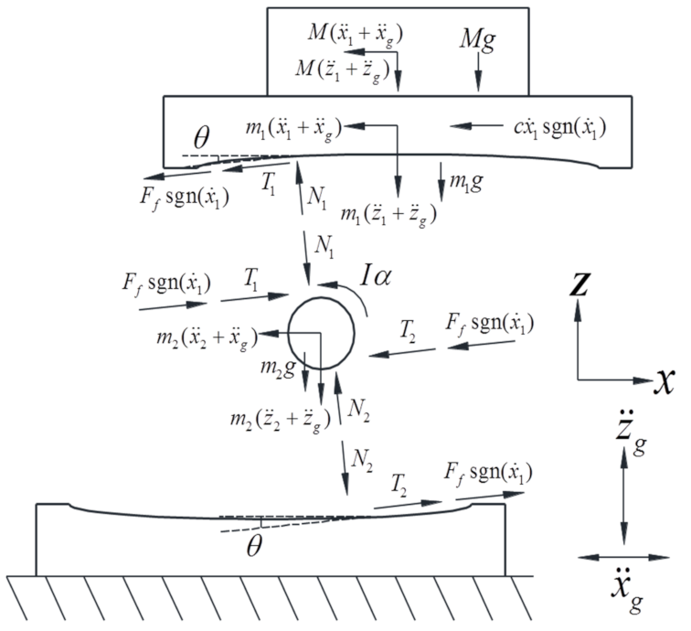
2.1. The Analytical Model for the Device

If more than three sets of rolling balls and curved surfaces are selected to form a pendulum bearing, it may happen that some rolling balls cannot fully come into contact with the upper support due to the errors of fabrication and assembly. Thus, three sets of single pendulum systems are incorporated in the newly proposed device, in which the multiple single pendulum systems are deliberately designed to behave independently. Meanwhile, these three sets of single pendulum bearings are configurated in detail to ensure the horizontal translation of the upper support plate. To figure out the dynamic behavior of this novel pendulum bearing, a simplified analytical model of the single pendulum system is firstly presented, taking advantage of the symmetrical configurations. As shown in Figure 2, the ball will keep rolling (in the pure rolling state) between the upper and lower support plates during an earthquake. As for the horizontally mounted viscous damper, the angle between the viscous damper and the upper support plate hardly changes and can be ignored.

2.2. The Restoring Force

In the analytical model, all the members are assumed to be rigid bodies, i.e., regardless of their deformation. The lower support plate is directly mounted on the ground, while the upper plate supports the equipment or cultural relics through additional connecting configurations. Given that the contact type between the ball and the curved surface is pure rolling, the displacement and velocity of the upper support plate ($x_1$, ${\dot{x}}_1$) and the ball ($x_2$, ${\dot{x}}_2$) should be in the same direction. Thus, the sign-function is introduced to describe this typical relationship:

$$sgn\left(x_1\right)=\left\{\begin{array}{c}\begin{array}{cc}1& x_1>0\end{array}\\ \begin{array}{cc}0& x_1=0\end{array}\\ \begin{array}{cc}-1& x_1<0\end{array}\end{array}\right.$$

(1)

$$sgn\left({\dot{x}}_1\right)=\left\{\begin{array}{c}\begin{array}{cc}1& {\dot{x}}_1>0\end{array}\\ \begin{array}{cc}0& {\dot{x}}_1=0\end{array}\\ \begin{array}{cc}-1& {\dot{x}}_1<0\end{array}\end{array}\right.$$

(2)

As mentioned above, the velocity-related type (viscous) dampers are selected for the device, and the typical force–velocity constitutive model can be expressed as follows:

$$F_c=c{v}^{\beta }$$

(3)

where F_c is the damping force, c is the damping coefficient, v is the velocity of the piston, and β is the velocity index. Considering the linear damping, the velocity index is set to one.

In order to figure out the mechanism inside the single pendulum system, the analytical model should be decomposed into three independent balanced bodies. As shown in Figure 3, M, m₁ and m₂ are the mass of the equipment being isolated, the upper plate and the rolling ball, respectively; g is the gravitational acceleration; ${\ddot{x}}_g$ and ${\ddot{z}}_g$ are the horizontal and vertical seismic accelerations, respectively; ${\ddot{x}}_1$ and ${\ddot{x}}_2$ are the relative horizontal accelerations of the upper plate and the rolling ball, respectively; ${\ddot{z}}_1$ and ${\ddot{z}}_2$ are the relative vertical accelerations of the upper plate and the rolling ball, respectively; T₁ and T₂ are the tangential contact forces between the ball and the upper and lower plates, respectively; N₁ and N₂ are the normal contact forces between the ball and the upper and lower plates, respectively; F_f is rolling friction force between ball and curved surface; c is the damping coefficient; I is the inertia moment of the ball; α is the angular acceleration of the ball; θ is the tangent contact angle between the ball and the curved surface.

Considering the force and geometric relationships between the three independent components, the following equations can be obtained:

$$\sum F_x=\left(M+m_1\right)\left({\ddot{x}}_1+{\ddot{x}}_g\right)=-T_{1}cos\theta -N_{1}sin\theta sgn(x_1)-c{\dot{x}}_{1}sgn\left({\dot{x}}_1\right)-F_{f}cos\theta sgn\left({\dot{x}}_1\right)$$

(4)

$$\sum F_z=\left(M+m_1\right)\left({\ddot{z}}_1+{\ddot{z}}_g\right)=-T_{1}sin\theta sgn\left(x_1\right)-N_{1}cos\theta -\left(M+m_1\right)g-F_{f}sin\theta sgn\left({\dot{x}}_1\right)$$

(5)

$$\sum F_x=m_2\left({\ddot{x}}_1+{\ddot{x}}_g\right)=T_{1}cos\theta -T_{2}cos\theta +N_{1}sin\theta sgn\left(x_1\right)-N_{2}sin\theta sgn\left(x_1\right)$$

(6)

$$\sum F_z=m_2\left({\ddot{z}}_1+{\ddot{z}}_g\right)=T_{1}sin\theta sgn\left(x_1\right)-T_{2}sin\theta sgn\left(x_1\right)-N_{1}cos\theta +N_{2}cos\theta -m_{2}g$$

(7)

$${\displaystyle \sum M=I\alpha =T_{1}r+}{T}_{2}r$$

(8)

$${\ddot{x}}_2=r\alpha cos\theta$$

(9)

$${\ddot{z}}_2=r\alpha sin\theta sgn\left(x_1\right)$$

(10)

$${\ddot{x}}_1={\ddot{x}}_2+r\alpha cos\theta =2r\alpha cos\theta$$

(11)

$${\ddot{z}}_1={\ddot{z}}_2+r\alpha sin\theta sgn\left(x_1\right)=2r\alpha sin\theta sgn\left(x_1\right)$$

(12)

Rearrange the Equations (4)–(11) so that the nine unknown variables, including ${\ddot{x}}_1$, ${\ddot{x}}_2$, ${\ddot{z}}_1$, ${\ddot{z}}_2$, N₁, N₂, T₁, T₂ and $\alpha$, can be decoupled from the known variables. It is obvious that the mass of the rolling ball is much smaller than the mass of the upper support plate, so that $m_2/\left(M+m_1\right)\approx 0$. Based on this simplification, Equations (4)–(12) can be rewritten as follows:

$${\ddot{x}}_1=-\frac{1}{2}\left({\ddot{z}}_g+g\right)sin2\theta -\frac{F_{f}cos\theta sgn\left({\dot{x}}_1\right)}{M+m_1}-\frac{c{\dot{x}}_{1}sgn\left({\dot{x}}_1\right)}{M+m_1}-{\ddot{x}}_g$$

(13)

$${\ddot{x}}_2=-\frac{1}{4}\left({\ddot{z}}_g+g\right)sin2\theta -\frac{F_{f}cos\theta sgn\left({\dot{x}}_1\right)}{2\left(M+m_1\right)}-\frac{c{\dot{x}}_{1}sgn\left({\dot{x}}_1\right)}{2\left(M+m_1\right)}-\frac{1}{2}{\ddot{x}}_g$$

(14)

$${\ddot{z}}_1=-\frac{1}{2}{\ddot{x}}_{g}sin2\theta sgn\left(x_1\right)-\frac{c{\dot{x}}_{1}sin2\theta sgn\left({\dot{x}}_1\right)sgn\left(x_1\right)}{2\left(M+m_1\right)}-\frac{F_{f}sin\theta sgn\left({\dot{x}}_1\right)sgn\left(x_1\right)}{M+m_1}$$

(15)

$${\ddot{z}}_2=-\frac{1}{4}{\ddot{x}}_{g}sin2\theta sgn\left(x_1\right)-\frac{c{\dot{x}}_{1}sin2\theta sgn\left({\dot{x}}_1\right)sgn\left(x_1\right)}{4\left(M+m_1\right)}-\frac{F_{f}sin\theta sgn\left({\dot{x}}_1\right)sgn\left(x_1\right)}{2\left(M+m_1\right)}$$

(16)

$$N_1=\left(M+m_1\right)\left[\left({\ddot{z}}_g+g\right)cos\theta -{\ddot{x}}_{g}sin\theta sgn\left(x_1\right)\right]+c{\dot{x}}_{1}sin\theta sgn\left({\dot{x}}_1\right)sgn\left(x_1\right)$$

(17)

$$N_1=\left(M+m_1+m_2\right)\left[\left({\ddot{z}}_g+g\right)cos\theta -{\ddot{x}}_{g}sin\theta sgn\left(x_1\right)\right]+c{\dot{x}}_{1}sin\theta sgn\left({\dot{x}}_1\right)sgn\left(x_1\right)$$

(18)

$$T_1=-\frac{m_2\left\{\left(M+m_1\right)\left[{\ddot{x}}_{g}cos\theta +sgn\left(x_1\right)\left({\ddot{z}}_g+g\right)sin\theta \right]-3F_{f}sgn\left(\dot{x}\right)\right\}}{8\left(M+m_1\right)+3m_2}$$

(19)

$$T_2=-\frac{m_2\left\{F_{f}sgn\left(\dot{x}\right)-\left[3\left(M+m_1\right)+m_2\right]\left[{\ddot{x}}_{g}cos\theta +\left({\ddot{z}}_g+g\right)sgn\left(x_1\right)sin\theta \right]\right\}}{8\left(M+m_1\right)+3m_2}$$

(20)

$$\alpha =-\frac{\left(M+m_1\right)\left[\left({\ddot{z}}_g+g\right)sin\theta sgn\left(x_1\right)-{\ddot{x}}_{g}cos\theta \right]+\left(c{\dot{x}}_{1}cos\theta +F_f\right)sgn\left({\dot{x}}_1\right)}{2r\left(M+m_1\right)}$$

(21)

According to Equation (13), the maximum horizontal absolute acceleration of the upper support plate can be expressed as follows:

$${\ddot{x}}_g+{\ddot{x}}_1+\frac{1}{2}{\ddot{z}}_{g}sin2\theta =-\frac{1}{2}gsin2\theta -\frac{F_{f}cos\theta sgn\left({\dot{x}}_1\right)}{M+m_1}-\frac{c{\dot{x}}_{1}sgn\left({\dot{x}}_1\right)}{M+m_1}$$

(22)

If the rolling friction force and viscous damping force are omitted, the restoring force of the upper plate in the horizontal direction can be obtained:

$$F^{\prime }=-\frac{1}{2}\left(M+m_1\right)gsin2\theta$$

(23)

According to Equation (23), the horizontal restoring force of the upper plate depends on the angle θ and the mass of the upper plate and the equipment (M and m₁).

After determining the horizontal restoring force, the characteristics of the curved surfaces, i.e., the geometric relationship between the horizontal displacement of the upper plate x₁ and the angle θ, should be figured out in the following sections.

2.3. The Surface Functions

It should be noted the spherical and elliptic surfaces are quite popular in the traditional pendulum-type bearings. Thus, the novel variable-frequency surface is presented to make comparisons with the traditional spherical surfaces. In fact, the natural period of the pendulum-type bearing depends on the radius of curvature. Hence, the surface function and the corresponding radius of curvature are selected as comparison indicators.

2.3.1. Traditional Spherical Surface

The functions of the spherical surface and the corresponding radius of curvature can be expressed as follows:

$$y\left(x\right)=R-\sqrt{R^2-x^2}$$

(24)

$$y^{\prime }\left(x\right)=\frac{x}{\sqrt{R^2-x^2}}$$

(25)

where R is the radius of curvature. According to Equation (25), the surface tends to be flatter with the growth of the radius of curvature.

2.3.2. Traditional Elliptic Surface

The functions of the elliptic surface and the corresponding radius of curvature can be expressed as follows:

$$y\left(x\right)=b-\frac{b\sqrt{a^2-x^2}}{a}$$

(26)

$$y^{\prime }\left(x\right)=\frac{bx}{a\sqrt{a^2-x^2}}$$

(27)

where a and b are the major and minor axes of the ellipse, respectively. Based on the relevant mathematical theories, the elliptic surface tends to be flatter with the growth of the major axis or the decline of the minor axis.

2.3.3. Variable-Frequency Surface

The variable-frequency pendulum bearing is firstly proposed by Pranesh et al. [33]. The functions of the variable-frequency surface and the corresponding radius of curvature originate from the elliptic function, and can be expressed as follows:

$$y\left(x\right)=b\left(1-\frac{\sqrt{d^2-2d\left|x\right|}}{d+\left|x\right|}\right)$$

(28)

$$y^{\prime }\left(x\right)=\frac{bdx}{{\left(d+\left|x\right|\right)}^2\sqrt{d^2-2d\left|x\right|}}$$

(29)

where b is the minor axes of the ellipse, and d is a constant that depends on the major axis of the ellipse and the displacement of the isolator. Pranesh et al. [34] have demonstrated that the initial slope of the variable-frequency surface is responsible for the initial period of the isolator and tends to be smaller with the growth of the constant d, or the decline of the minor axis.

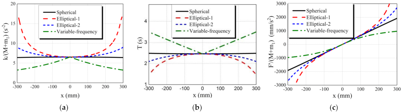
2.4. Comparison of the Device Characteristics with Different Curved Surfaces

The previous sections have given a detailed description of the three different curved surfaces, including the spherical surface, the elliptic surface, and the variable frequency surface. Assuming the second-order derivative of the surface function exists, the relationship between the angle θ and the displacement of the lower plate x₂ can be directly determined based on the gradient of the surface. Then the relationship between the angle θ and the displacement of the upper plate x₁ can also be determined. In order to make a valid comparison between the different pendulum bearings, the initial period is set to 2.5 s, i.e., the initial radius of curvature is 750 mm. In terms of the variable-frequency surface, special importance should be attached to the choice of the parameters to ensure the same restoring force. Meanwhile, two sets of elliptic surfaces are introduced to consider the effect of the limit displacement. The key parameters of the four pendulum bearings are listed in

Table 1. The key parameters of four pendulum bearings (Unit: mm).

Surface Classification	Spherical Surface	Elliptic Surface 1	Elliptic Surface 2	Variable Frequency Surface
Initial period T = 2.5 s	R = 750	a = 150 and b = 30	a = 200 and b = 53	b = 300 and d = 473

. Moreover, the comparisons of geometry and slope between the four pendulum bearings are also conducted, as shown in Figure 4.

2.5. Mechanical Characteristic of the Four Pendulum Bearings

2.5.1. The Stiffness, Natural Period and Horizontal Restoring Force

If the rolling friction force and viscous damping force are omitted, the restoring force of the upper plate in the horizontal direction F′ can be simulated by the variable-stiffness spring. Based on Equation (23), the stiffness and period of the pendulum bearing can be expressed as follows:

$$k=\frac{F^{\prime }}{x_1}=\frac{gsin2\theta \left(M+m_1\right)}{2x_1}=\frac{gsin\theta cos\theta \left(M+m_1\right)}{x_1}$$

(30)

$$T=2\pi \sqrt{\frac{\left(M+m_1\right)}{k}}$$

(31)

It should be emphasized that the natural period of the proposed device is independent of the mass of the equipment being isolated. According to Equations (30) and (31), the comparisons of $\frac{k}{\left(M+m_1\right)}-x_1$, $T-x_1$ and $\frac{F^{\prime }}{\left(M+m_1\right)}-x_1$ between the four pendulum bearings mentioned in Table 1 are displayed in Figure 5.

As shown in the three comparison charts, the stiffness and period of the spherical surface remain basically unchanged with the growth of x₁, while the horizontal restoring force increases linearly. As for the elliptic surface, the stiffness becomes larger and the period declines with the growth of x₁. The restoring force of the elliptic surface is similar to that of the spherical surface to some extent and changes rapidly when the rolling ball reaches the boundary of the curved surface. Furthermore, the period and the restoring force of the variable-frequency surface increases with the growth of x₁, while the stiffness becomes smaller. It is worth mentioning that the characteristics of the variable-frequency surface change rapidly in the initial phase and gradually tend to a steady state.

In summary, the proposed variable-frequency pendulum bearing has a stiffness softening mechanism that decreases stiffness as the displacement increases. Compared with spherical and elliptic surfaces, the variable-frequency pendulum bearing has the potential to preclude undesirable resonance effects resulting from the low-frequency ground motion amplification.

2.5.2. The Hysteretic Performance

It is worth mentioning that the effect of the rolling friction is not considered for the sake of simplification in the previous sections. When the rolling friction F_f is considered during the calculation of the horizontal force, Equations (16) and (17) can be rearranged as follows:

$$F_f=\left\{\left(M+m_1\right)\left[\left({\ddot{z}}_g+g\right)cos\theta -{\ddot{x}}_{g}sin\theta sgn\left(x_1\right)\right]+c{\dot{x}}_{1}sin\theta sgn\left({\dot{x}}_1\right)sgn\left(x_1\right)\right\}\mu$$

(32)

where μ is the coefficient of rolling friction. The coefficient of rolling friction is usually small and can be set to 0.005. Equation (32) was simplified since the sum of the masses of the upper plate and the isolated equipment (M + m₁) is far larger than the mass of the rolling ball m₂. According to Equation (32), the rolling friction depends on the M, m₁ and μ.

When the rolling friction force is added to the horizontal force (the viscous damping force is omitted), the theoretical hysteresis curves of the four pendulum bearings (shown in Figure 6) can be obtained by assuming that the pendulum bearing has the same movement locus whether in the positive or negative direction.

As shown in Figure 6, the energy dissipation performance of all the four pendulum bearings is poor when the rolling friction is considered. Thus, additional dampers are introduced to improve the energy dissipating capacity by increasing the system damping. Furthermore, the stiffness of the variable-frequency pendulum bearing declines with the increasing displacements, and the horizontal restoring force tends to be saturated which precludes the transmission of the large shear force.

2.5.3. The Self-Restoring Performance

It is well established that the pendulum bearing with a detailed configuration can restore to its initial position after an earthquake. Due to the dead load and the characteristics of the curved surface, the pendulum bearing usually can generate a self-restoring force F_r. Only if the self-restoring force F_r is larger than the friction force F_f can the rolling ball restore to the original position at low speeds. In this situation, the velocity of the rolling ball is usually small, i.e., the viscous damping force and can be omitted, and the horizontal and vertical seismic accelerations will be zero.

$$F_r=\frac{1}{2}gsin2\theta \left(M+m_1\right)\ge F_f=\mu gcos\theta \left(M+m_1\right)$$

(33)

According to Equation (33), only if sin θ ≥ μ can the pendulum bearing restore to the initial position. Given that θ is usually small, Equation (33) can be rewritten as tan θ ≥ μ, i.e.,

$$y^{\prime }\left(x\right)\ge \mu$$

(34)

Assuming the theoretical maximum residual displacement is x_c, Equation (34) can be replaced by $y^{\prime }\left(x_c\right)=\mu$. Thus, the theoretical maximum residual displacements of the four pendulum bearings are 3.75 mm, 3.75 mm, 3.77 mm, and 3.79 mm, respectively. It is obvious that all four pendulum bearings have small residual displacements, which indicates the distinguished self-restoring performance.

3. The Shake Table Tests

As previously mentioned, the variable-frequency pendulum bearings proposed in this paper can reduce the peak acceleration response of the equipment. In order to investigate their seismic performance under different configurations, the shake table tests are carried out. During the test, several measures, such as increasing the stiffness, the system damping and the self-restoring force and so on, are taken to mitigate the excessive displacements caused by long-period ground motions. These measures will be illustrated in the following sections.

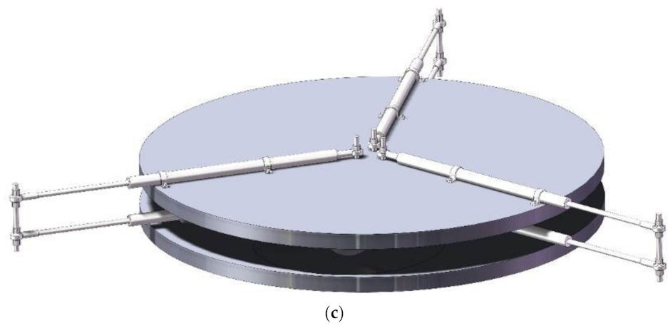
3.1. The Design of the Pendulum Bearings

3.1.1. The Key Parameters

According to Equation (28), the surface function of the variable-frequency pendulum bearing is controlled by the minor axes of the ellipse b, and the displacement dependent parameter d. As mentioned above, the surface function tends to be saturated and the initial stiffness becomes smaller with the growth of parameter b or the decline of parameter d. Considering the velocity-related damping coefficient c, there are three parameters to be taken into account in the variable-frequency pendulum bearing. Thus, four sets of variable-frequency pendulum bearings have been configured in detail to investigate the effects of the three parameters on the seismic response of the pendulum bearings. The detailed information of the four variable-frequency pendulum bearings is listed in

Table 2. The key parameters of the four variable-frequency pendulum bearings.

Parameter	b200d250	b200d380	b300d380	b200d380-c
b (mm)	200	200	300	200
d (mm)	250	380	380	380
c (N∙s/m)	100	100	100	150
Initial period (s)	1.6	2.4	2.0	2.5

. Moreover, the stiffness and period comparisons of the four variable-frequency pendulum bearings are shown in Figure 7.

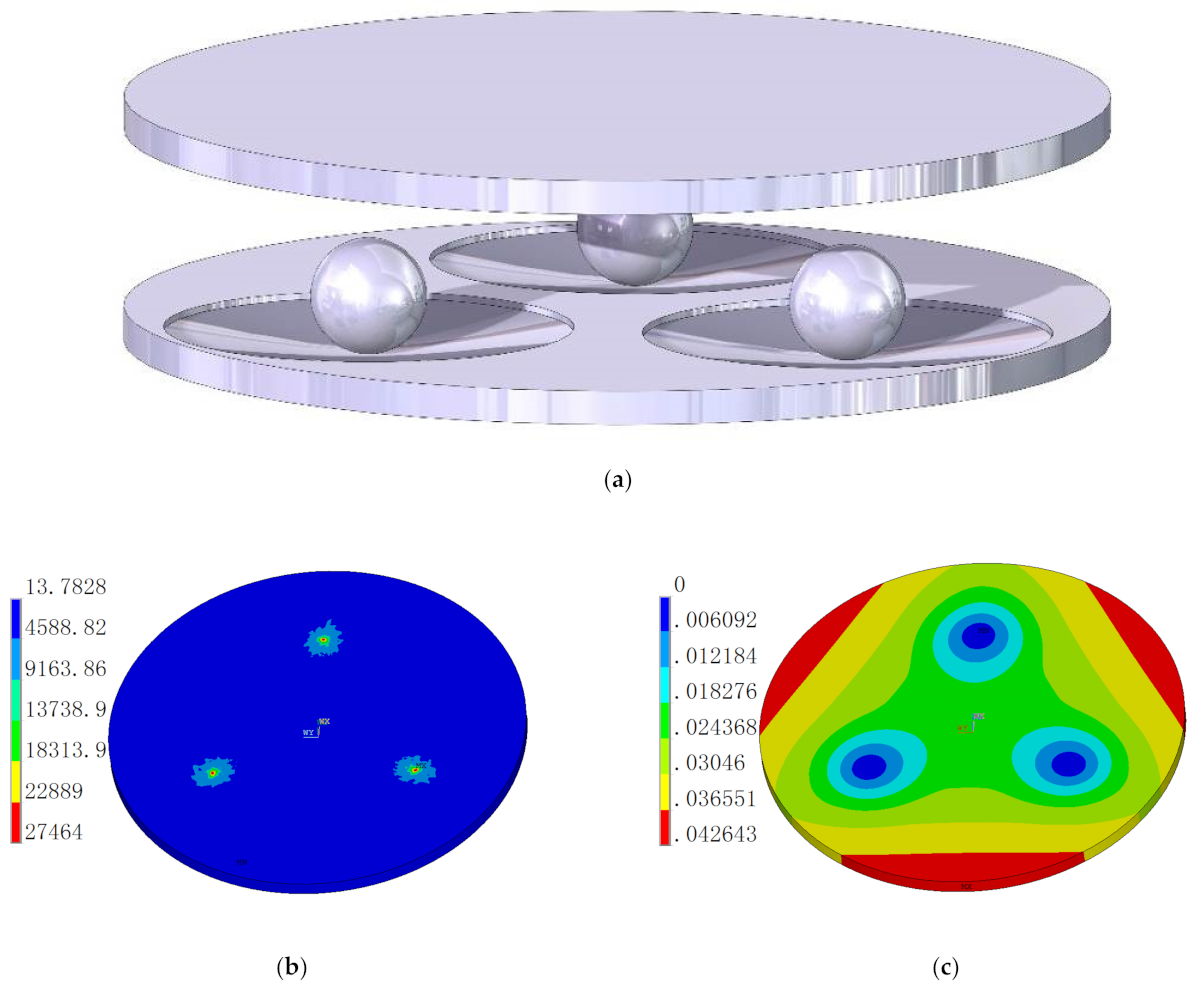
3.1.2. The Support Plates and the Rolling Sphere

Once the curved surface was determined, the next step is to design the support plate. As shown in Figure 8a, there are three sets of curved surfaces uniformly distributed on the upper and lower support plates, whose diameter is set to 300 mm. The diameter of the upper and lower support plates is set to 720 mm. The high-strength steel Q345 is selected as the material for the support plate. Moreover, the depth of the curved surface was increased by 5 mm to limit the rolling ball. Based on the surface function mentioned above, the maximum depth of the curved surface is less than 15 mm. Hence, the thickness of the support plate is set to 25 mm to ensure that the thickness in the thinnest region is not less than 5 mm.

To check the strength and deformation capacity of the upper support plate, the complementary finite element simulation was conducted with the aid of Ansys software. Solid45 elements are utilized to model the device, and the equivalent surface pressure is applied to the upper plate to imitate the weight of the isolated equipment (200 kg). Meanwhile, the lower plate is fixed to the ground to provide a static boundary condition. The simulated results (see Figure 8b,c) demonstrate that the stress and deformation of the upper support plate are very small, which satisfies the performance requirements.

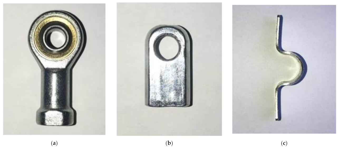
3.1.3. The Viscous Damper

As mentioned in the previous sections, the energy dissipation performance of the pendulum bearing alone is poor. Thus, the linear viscous dampers are added to the pendulum bearings. It is worth mentioning that the design diameter of the curved surface is 300 mm. In view of the ball size, the design displacement of the rolling ball is set to ±125 mm, so the design displacement of the upper plate should be set to ±250 mm. Considering the large diameter and design displacement of the upper plate, two sets of bidirectional linear viscous dampers with a single stroke of ±125 mm (see Figure 9b) are connected in parallel to form a damper system, instead of a traditional damper with a stroke of ±300 mm (see Figure 9a).

To facilitate the application in actual engineering, the size of the isolation bearing should be configured as small as possible while ensuring the effective performance. Hence, the dampers are designed to connect the support plate in the central region of the support plate. Considering the typical configurations of the pendulum bearings proposed in this paper, the fisheye and flat round joints (see Figure 10a,b) are utilized in the connection regions to facilitate the free motion of the device. Meanwhile, the casing clamps (see Figure 10c) are introduced to fix the dampers on the upper plate, which precludes the collisions between the dampers and the rolling balls. Furthermore, in order to ensure sufficient damping in every direction, three sets of damping transmission systems are applied to the pendulum bearing (see Figure 10a). The rubber gaskets are also adopted in the joint between the dampers and the lower plate to reduce the in-plane torsional response of the upper plate. Figure 11a–c shows the detailed configurations of the dampers and the support plates.

3.1.4. The Rolling Ball and the Rolling Friction

The rolling ball is also made of steel, and the diameter is set to 85 mm to provide enough space for the dampers placed between the upper and lower support plates. Meanwhile, the surface of the rolling ball is sanded (see Figure 12a) to preclude the pure slipping between the rolling ball and the curved surface.

Given that the rolling friction is influenced by many factors, there is currently no appropriate model that can accurately calculate the rolling friction coefficient. In most cases, the rolling friction coefficient is determined by performing an indirect measurement. Li et al. [35] has devised a technique that can accurately calculate the rolling friction coefficient through formulas, in which the relevant data can be easily measured using conventional distance angle measurement tools. During the measurement, SPC (Statistical Process Control) testing is adopted to check the validity of the data. Moreover, the discrete element simulations have been conducted to verify the accuracy of the method.

In this paper, the actual measurement method proposed by Li et al. [35] is adopted to determine the rolling friction coefficient. As shown in Figure 12b, the length L, angle θ and height h₁ of the inclined plane, the height of the cabinet h₂, and the horizontal distance of the ball drop point from the cabinet H are measured in each test. Each test should be repeated at least 30 times, and the corresponding data will be tested for normality. Finally, the rolling friction coefficient μ can be expressed as follows:

$$\mu =\frac{\left\{h_1-H^2/\left[4{cos}^2\theta \left(h_2-Htan\theta \right)\right]\right\}}{Lcos\theta }$$

(35)

As shown in Figure 12c, a slope is configured using the same material and surface as the isolation bearing to reproduce the surroundings of the rolling ball. Given that the rolling ball in the isolation bearing is too large to be directly used for the measurement of the rolling friction coefficient, a smaller ball with the same material and roughness is adopted for the series tests. Based on the afore-mentioned method, the test was repeated 44 times, and the SPC method was also introduced using MATLAB software to determine whether the data are normally distributed. According to the experimental results, the rolling friction coefficient μ between the ball and the support plates is 0.01.

3.1.5. The Issues Regarding Limit, Overturning and Torsion

The pendulum bearings are usually configured to decouple the structure from the ground motions during earthquakes by sacrificing displacement response. However, the displacement sometimes may be too large, or even exceed the design displacement threshold for certain ground motions. Moreover, much importance is usually attached to mitigating the undesirable effects resulting from horizontal seismic excitations or vertical bearing capacity issues, while the overturning mode is often ignored. Once the horizontal displacement is relatively large followed by vertical load, the pendulum bearing may cause failure due to the overturning mode.

The pendulum bearings proposed in this paper can restrain the rolling ball by the deep cut of the support plates and the design stroke of the viscous dampers. As for the overturning, the three sets of dampers incorporated to rolling pendulum bearing can effectively avoid it without any effort. Furthermore, the surface characteristic of the pendulum bearing can also mitigate the torsion effect to some extent. Meanwhile, the rubber washer is used on the connection between the damper and the lower support plate to dissipate the energy generated by the twist.

3.1.6. The Issues Regarding Manufacturing and Assembly Installation

In the actual manufacturing, the pendulum bearing may not often get the expected results due to the errors of the manufacturing and the assembly installation. Hence, VMC-series machine tools (see Figure 13a) are introduced to machine the upper and lower support plates. VMC-series machine tools are known for the accurate vertical machining in the field of the mold manufacturing, and the maximum load capacity of the worktable is 320 kg, which can almost satisfy the requirements of milling, drilling, tapping, boring and other machining processes. Meanwhile, the three-dimensional models of the support plates have been built to facilitate CNC machining during the vertical machining process (see Figure 13b).

It should be noted that the biggest error during assembly installation lies in the placement of the upper support plate. Given the three rolling balls, it is often difficult to align the upper support plate to the lower support plate. Thus, three pairs of positioning holes are placed on the upper and lower support plates to improve the centering accuracy. In order to preclude the moving of the rolling ball during installation, the rubber strip is utilized to place the ball at the center of the curved surface. Once the ball starts to bear the vertical load, the rubber strip will be removed. The detailed description of the installation process of the support plate is shown in Figure 14.

3.2. The Shake Table

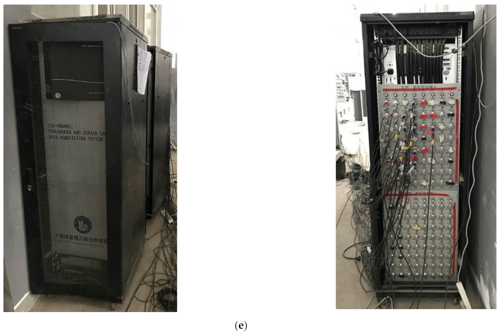
3.2.1. Shake Table Apparatus

The shake table tests were conducted in the Key Laboratory of Earthquake Engineering and Engineering Vibration of China Earthquake Administration. The shake table used in this test (see Figure 15a) is a 6-DOF facility with a table dimension of 3.5 m by 3.5 m, and the maximum displacement in horizontal and vertical directions are 0.025 m and 0.02 m, respectively. Its maximum speeds in horizontal and vertical directions are 2.4 m/s and 1.8 m/s, respectively. Meanwhile, the maximum accelerations in longitudinal, transverse, and vertical directions are 4 g, 4 g, and 3 g, respectively. Its maximum overturning moment is 400 kN·m and the maximum payload is 60 kN. Detailed parameters of this facility are present in Ning et al. [36]. The arrangement of the test models on the shake table is shown in Figure 15b.

3.2.2. Arrangement of Data Acquisition Points

Two types of sensors, including accelerometers, and displacement transducers, were installed on the model so that the isolation efficiency of the pendulum bearing could be measured. The isolation efficiency of the pendulum bearing can be defined as follows:

$$\mathrm{Isolation}\mathrm{efficiency}=\left(1-\frac{\max \mathrm{acceleration}\mathrm{with}\mathrm{isolation}}{\max \mathrm{acceleration}\mathrm{without}\mathrm{isolation}}\right)\times 100\%$$

(36)

According to Equations (30) and (31), the natural period of the proposed device is independent of the mass of the equipment being isolated. Meanwhile, the equipment is usually fixed to the upper plate, namely, the isolated equipment and upper plate have the same acceleration responses. Thus, the model of the equipment was not placed separately during the test, for the sake of simplicity. In this situation, the seismic responses of the upper plate are utilized for the following analysis.

Totally, there were five piezoelectric acceleration sensors, including one sensor built-in laboratory shake table system and four external acceleration sensors used to monitor the acceleration responses of the pendulum bearings (see Figure 16a). The acceleration sensors (see Figure 16c) were placed on the shake table and the upper support plates of the pendulum bearings, Meanwhile, 12 drawing displacement sensors with ranges of 0∼±200 mm (see Figure 16d) were utilized to measure the relative displacements between specimens and the shake table, so as to analyze the trajectory of the center of the isolated equipment. Distributions of some accelerometers and drawing displacement sensors are shown in Figure 16b. As shown in Figure 16e, the measured data were recorded by Pacific Collector during tests.

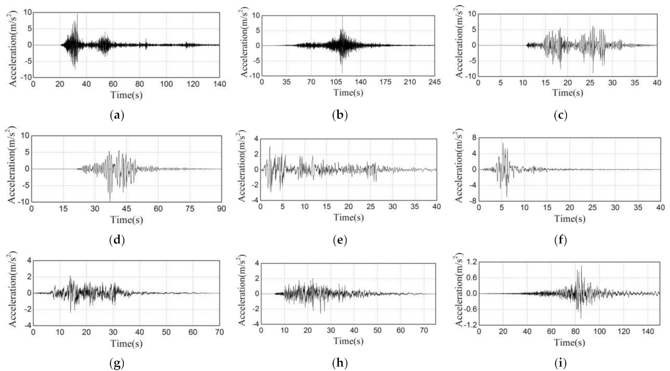
3.2.3. Selecting and Scaling Ground Motion Records

In order to verify the isolation efficiency of the device, three different types of ground motions were selected as input accelerations to the test: (a) the short-period (high-frequency) ground motions, (b) the intermediate-frequency ground motions, and (c) the long-period (low-frequency) ground motions. There is no specific definitions or gaps among these three ground motions. They are selected by ground motion-dominant frequencies and grouped by experiences. The detailed information of the ground motions is listed in

Table 3. The detailed information of the input ground motions.

	Input Ground Motion	Magnitude	Occurrence Time	Station	PGA (m/s2)	Time Interval (s)	Total Time (s)
High-frequency	Wo-long	8.0	2008	051WCW	9.58	0.005	75
	311	9.0	2011	IBR005	9.67	0.01	100
	IZMIT	7.4	1999	Lamont375	8.90	0.01	40
Intermediate-frequency	ChiChi-TCU084	7.6	1999	TCU084	10.09	0.005	75
	ELcentro-BCJ	7.1	1940	BCJ	3.05	0.02	54
	Kobe	6.9	1995	Takarazuka	6.94	0.005	51
Low-frequency	ChiChi-TCU049	7.6	1999	TCU049	2.44	0.005	75
	ChiChi-TCU122	7.6	1999	TCU122	2.61	0.005	50
	061CHC	8.0	2008	061CHC	1.07	0.005	100

. Meanwhile, the time histories, the frequency spectrums of acceleration, and the response spectrums of acceleration, velocity, and displacement (damping 5%) are also shown in Figure 17 and Figure 18. It can be seen from Figure 18 that the predominant frequency of the high-frequency ground motion is generally greater than 1.5 Hz, and the major frequency components are higher than 1.5 Hz; the predominant frequency of the intermediate-frequency ground motion is approximately between 1 Hz~1.5 Hz; the predominant frequency of the low-frequency ground motion is less than 1.0 Hz, and the frequency component lower than 1.0 Hz accounts for the main component.

According to the Chinese Code for Seismic Design of Buildings (CSDB, GB 50011-2010) [37], three-dimensional inputs were used in the shake table tests, and the PGA ratio of the principal direction to the other two directions was set to 1:0.85:0.65 (vertical). Considering the seismic intensity of 8(9), the peak accelerations (PGAs) corresponding to earthquakes of minor, moderate, and major levels were specified to be 0.07 g (0.14 g), 0.2 g (0.4 g), and 0.4 g (0.62 g), respectively. In addition, the extremely rare strong earthquakes with a PGA of 1.0 g were added to investigate the isolation performance under extreme conditions. Meanwhile, the white noise excitation tests were introduced to measure the dynamic properties of the specimens. A total of 42 cases were conducted during tests and a summary of the inputs used for each test is presented in

Table 4. Test program of the pendulum bearings.

Test No.	Input Signal	PGA (m/s2)	Test No.	Input Signal	PGA (m/s2)
1	White noise	2.0	22	Elcentro-BCJ	0.7
2	Wo-long	0.7	23	Kobe	0.7
3	311	0.7	24	ChiChi-TCU084	1.4
4	IZMIT	0.7	25	ELcentro-BCJ	1.4
5	Wo-long	1.4	26	Kobe	1.4
6	311	1.4	27	ChiChi-TCU084	2.0
7	IZMIT	1.4	28	Elcentro-BCJ	2.0
8	Wo-long	2.0	29	Kobe	2.0
9	311	2.0	30	ChiChi-TCU084	4.0
10	IZMIT	2.0	31	Elcentro-BCJ	4.0
11	Wo-long	4.0	32	Kobe	4.0
12	311	4.0	33	White noise	2.0
13	IZMIT	4.0	34	ChiChi-TCU049	0.7
14	Wo-long	6.2	35	ChiChi-TCU122	0.7
15	311	6.2	36	061CHC	0.7
16	IZMIT	6.2	37	ChiChi-TCU049	1.4
17	Wo-long	10.0	38	ChiChi-TCU122	1.4
18	311	10.0	39	061CHC	1.4
19	IZMIT	10.0	40	ChiChi-TCU049	2.0
20	White noise	2.0	41	ChiChi-TCU122	2.0
21	ChiChi-TCU084	0.7	42	061CHC	2.0

.

3.3. Shake Table Test Results

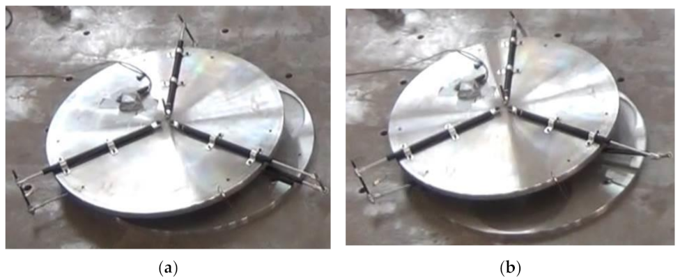
3.3.1. Test Phenomenon

At the beginning of the test, the upper support plate was observed to have slight vibration due to the vibration noise of the shake table facility. Meanwhile, as the PGA increases, the displacement responses of the upper support plate gradually became obvious (see Figure 19, Figure 20 and Figure 21). Furthermore, the displacement response of the upper support plate became larger when declining the predominant frequency of the ground motions, while keeping a constant PGA. When the pendulum bearing was within the design displacement threshold, overturning and twisting were not observed during the test. Hence, it could be concluded that the damper system proposed in the previous sections effectively solved the problem of damper travel as expected.

After each test, the pendulum bearings demonstrated distinguished self-restoring capacity and the rolling ball could almost restore to its original position. However, a few exceptions were observed in that some rolling balls could not fully return to the initial positions when the displacement response was too large. The sliding between the rolling ball and the curved surface can account for this phenomenon. Moreover, it will be easy for the ball to slide on the curved surface once the support plates cannot be aligned due to large manufacturing errors.

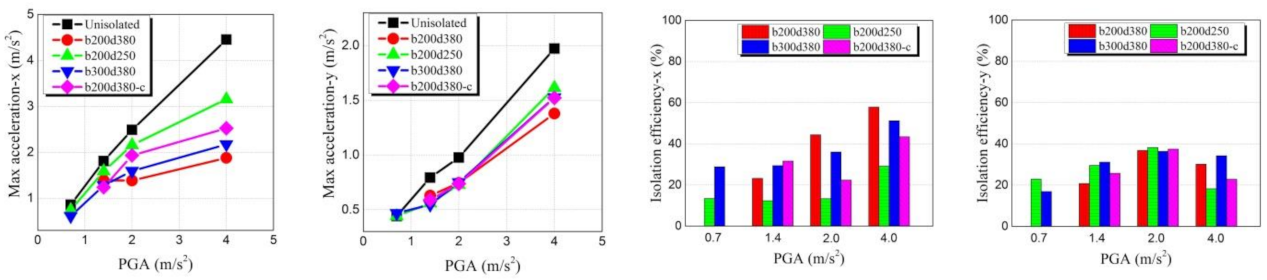
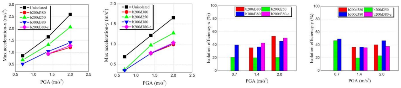
3.3.2. Acceleration Responses of the Devices

Given that the shake table did not work exactly according to the input accelerations, the accelerations recorded by the acceleration sensor placed on the shake table were utilized as the input accelerations. In the following sections, the effects of the three factors, including (1) the ground motions, (2) the damping parameters, and (3) the surface function parameters, on the acceleration isolation efficiency will be discussed based on the results of the shake table tests. Due to the space limitation, only several representative tests will be discussed in detail.

Figure 22 compares the horizontal accelerations between the equipment with the b300d380 pendulum bearing and without isolation subjected to three high-frequency ground motions at PGA of 0.7 m/s² and 10 m/s². It can be observed that when the PGA is set to 0.7 m/s², the maximum acceleration response of the device in the x-direction subjected to Wo-long, 311, and IZIMIT ground motions decreases by 61%, 69%, and 75%, respectively, while the acceleration response in the y-direction decreases by 62%, 44%, and 62%, respectively; when the PGA is set to 10 m/s², the maximum acceleration response of the device in the x-direction subjected to Wo-long, 311, and IZIMIT ground motions decreases by 70%, 82%, and 89%, respectively, while the acceleration response in the y-direction decreases by 62%, 72%, and 80%, respectively. Thus, it can be concluded that the variable-frequency rolling pendulum bearings exhibit excellent isolation performance under the high-frequency ground motions and the isolation efficiency increases as the PGA increases.

Figure 23 compares the horizontal accelerations between the equipment with the b300d380 pendulum bearing and without isolation subjected to three intermediate-frequency ground motions at PGA of 0.7 m/s² and 4 m/s². It can be observed that when the PGA is set to 0.7 m/s², the maximum acceleration response of the device in the x-direction subjected to ChiChi-TCU084, ELcentro-BCJ and Kobe ground motions decreases by 29%, 50%, and 54%, respectively, while the acceleration response in the y-direction decreases by 31%, 41%, and 59%, respectively; when the PGA is set to 4 m/s², the maximum acceleration response of the device in the x-direction subjected to ChiChi-TCU084, ELcentro-BCJ and Kobe ground motions decreases by 51%, 69%, and 56%, respectively, while the acceleration response in the y-direction decreases by 34%, 58%, and 49%, respectively. Thus, it can be concluded that the variable-frequency rolling pendulum bearings exhibit ordinary isolation performance under the intermediate-frequency ground motions and the isolation efficiency also increases as the PGA increases.

Figure 24 compares the horizontal accelerations between the equipment with b300d380 pendulum bearing and without isolation subjected to three low-frequency ground motions with PGA of 0.7 m/s² and 2 m/s². It can be observed that at PGA 0.7 m/s², the maximum acceleration of the device in the x-direction subjected to ChiChi-TCU049, ChiChi-TCU122, 061CHC ground motions decreases by 47%, 40%, and 33%, respectively, while the acceleration response in the y-direction decreases by 37%, 49%, and 32%, respectively; when the PGA is set to 2 m/s², the maximum acceleration response of the device in the x-direction subjected to ChiChi-TCU049, ChiChi-TCU122, 061CHC ground motions decreases by 57%, 46%, and 32%, respectively, while the acceleration response in the y-direction decreases by 53%, 47%, and 27%, respectively. Thus, it can be concluded that the variable-frequency pendulum bearings exhibit satisfactory isolation performance under the low-frequency ground motions and the isolation efficiency almost stays the same with the growth of the PGA.

From the perspective of PGA decline, the b300d380 pendulum bearing becomes more efficient as the ground motion dominant frequency rises. Furthermore, three typical ground motions are selected to investigate the influence of the surface parameters and the additional damping on the acceleration response. Figure 25, Figure 26, Figure 27 and Figure 28 show the maximum acceleration responses of the four variable-frequency pendulum bearings and the shake table, which are subjected to Wo-long, ChiChi-TCU084, ChiChi-TCU122, and 061CHC ground motions with different PGAs. As mentioned above, the surface of the variable-frequency pendulum bearing is determined by the two parameters: d and b. To figure out the effects of the parameter d, a comparison between the b200d250 and the b200d380 pendulum bearings is conducted. It can be concluded that there is no obvious difference between the two devices under high-frequency ground motions, while under intermediate-frequency and low-frequency ground motions, the b200d380 bearing becomes more efficient than the b200d250 bearing, especially with the growth of the PGA. It should be emphasized that the b200d250 bearing exhibits poor isolation performance under the 061CHC ground motion, which can be attributed to: (a) the sliding between the rolling ball and the curved surface caused by the steep surface and large displacement; (b) the frequency closeness between the b200d250 bearing and the 061CHC ground motion.

As for the parameter b, the comparison results between the b200d380 and the b300d380 pendulum bearings demonstrate that: (a) there is no obvious difference in the isolation efficiency under the high-frequency ground motions; (b) under the medium- and low-frequency ground motions, the b200d380 bearing becomes more efficient than the b300d380 bearing, especially with the growth of the PGA.

Finally, the comparisons between the b200d380 and the b200d380-c pendulum bearings are conducted to analyze the effects of the damping parameter c. Under high-frequency ground motions, both the devices exhibit excellent isolation performance and there is no significant difference between them. Under medium- and low-frequency ground motions, the b200d380 bearing becomes more efficient than the b200d380-c bearing with the growth of the PGA.

Table 5. The isolation efficiency of the variable-frequency in some representative tests.

Input Ground Motion	PGA (m/s2)	b200d250		b200d380		b300d380		b200d380-c
		x	y	x	y	x	y	x	y
Wo-long	0.7	49%	61%	-	-	38%	33%	61%	62%
Wo-long	1.4	68%	78%	-	-	60%	56%	65%	84%
Wo-long	2.0	70%	64%	67%	62%	68%	65%	80%	79%
Wo-long	4.0	78%	75%	80%	79%	79%	75%	79%	83%
Wo-long	6.2	74%	74%	81%	80%	80%	77%	83%	84%
Wo-long	10.0	78%	74%	80%	80%	77%	74%	70%	63%
Wo-long-average		69%	71%	77%	75%	67%	63%	73%	76%
ChiChi-TCU084	0.7	13%	23%	-	-	-	-	29%	17%
ChiChi-TCU084	1.4	12%	30%	23%	21%	32%	26%	29%	31%
ChiChi-TCU084	2.0	13%	38%	44%	37%	22%	37%	36%	36%
ChiChi-TCU084	4.0	29%	18%	58%	30%	43%	23%	51%	34%
ChiChi-TCU084-average		17%	27%	42%	29%	32%	29%	36%	30%
ChiChi-TCU122	0.7	21%	47%	-	-	-	-	40%	49%
ChiChi-TCU122	1.4	20%	20%	37%	36%	43%	36%	37%	37%
ChiChi-TCU122	2.0	20%	23%	40%	38%	50%	38%	45%	47%
ChiChi-TCU122-average		20%	30%	38%	37%	47%	37%	41%	44%

lists the isolation efficiency of the variable-frequency rolling pendulum bearings under some representative tests.

As shown in Figure 22, Figure 23 and Figure 24, there are always some high-frequency noises on the acceleration responses of the shake table and the specimens. When the acceleration input is small, the maximum acceleration responses of the shake table and the specimens may not be extracted due to the coverage of the high-frequency noises, which results in little difference between the four variable-frequency pendulum bearings. The reasons for the significant impacts of high-frequency may be attributed to: (a) the point-surface contact between the rolling ball and the curved surface; (b) the misalignment of the support plates due to the installation errors or the sliding of the rolling ball during the test; (c) the unstable energy dissipating performance of the viscous dampers when the acceleration input level is small.

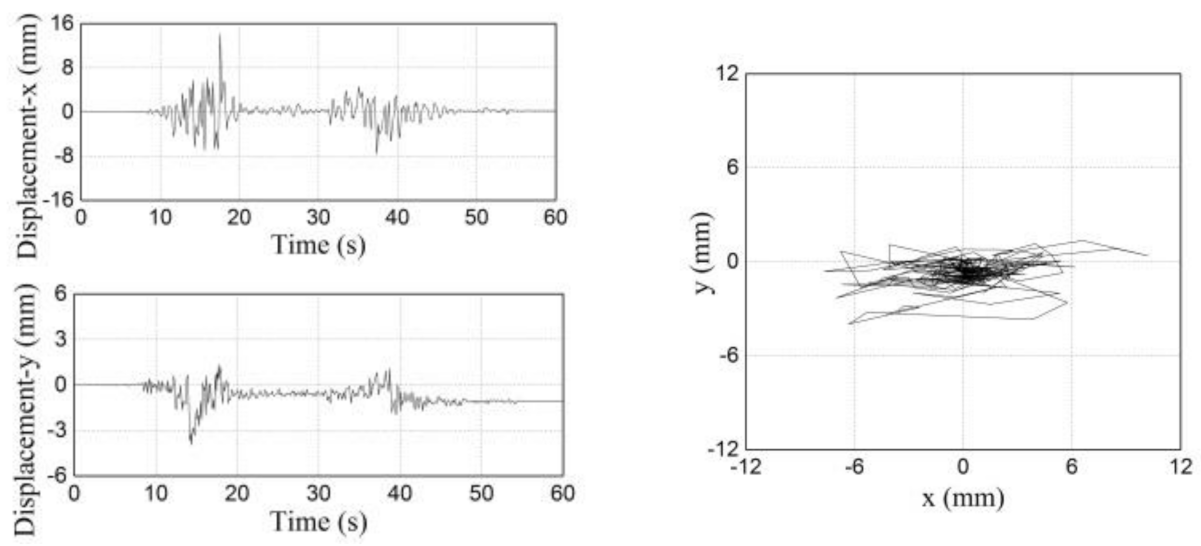
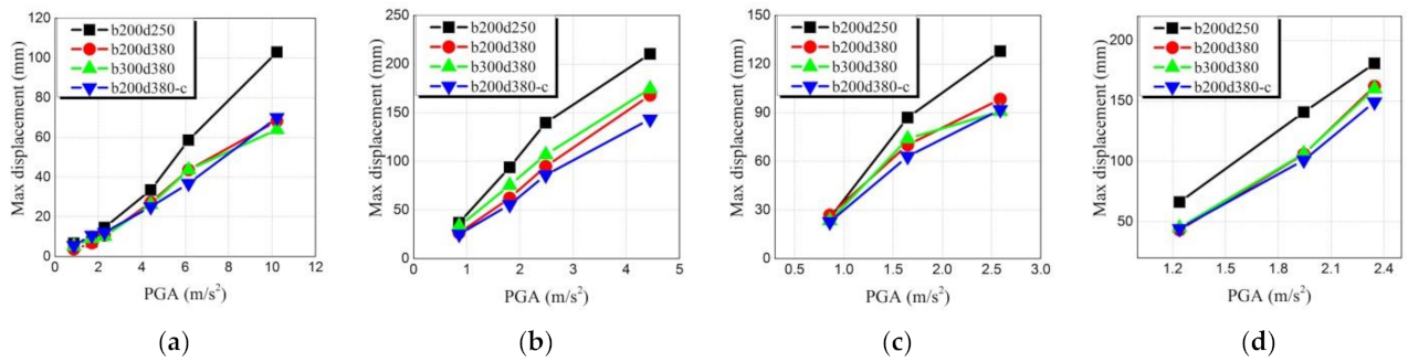
3.3.3. Displacement Responses of the Devices

The relative displacement responses of the pendulum bearings can be obtained through the data recorded by the displacement gauges. Then, the relative displacement responses can be utilized to investigate the effects of the ground motions, the damping coefficient, and the parameters of the surface function on the isolation efficiency. Due to the space limitation, only several representative tests are also discussed in detail.

Figure 29, Figure 30, Figure 31 and Figure 32 demonstrate the two-horizontal relative-displacement responses and the movement locus of the b200d380 bearing subjected to Wo-long (high-frequency), ChiChi-TCU084 (intermediate-frequency), ChiChi-TCU122 and 061CHC (low-frequency) with PGA of 2 m/s². It can be observed that the relative-displacement amplitudes decrease with the growth of the predominant frequency of the ground motions. Meanwhile, the displacement responses demonstrate that there is almost no residual displacement, which indicates the distinguished self-restoring performance of the b200d380 bearing.

Figure 33a–d show the maximum relative-displacement responses (in the x-direction) of the four variable-frequency pendulum bearings subjected to Wo-long, ChiChi-TCU084, ChiChi-TCU122 and 061CHC ground motions with different PGAs. It can be found that the displacement of the b200d250 bearing is large, which may be attributed to the slipping between the rolling ball and the curved surface. Moreover, appropriately increasing the damping coefficient is beneficial for the reduction of the maximum displacement response. However, there will be no obvious difference between the maximum displacement responses of the variable-frequency pendulum bearings, whether the parameter b is set to 0.2 m or 0.3 m.

4. The Numerical Analysis

It is impractical to do shake table tests for all circumstances. Numerical analysis is an excellent supplement to tests. Universal finite element software, such as ANSYS and Abaqus, is sometimes time-consuming, especially when complex models are involved. A numerical model of the isolation system based on MATLAB is proposed that can be used for additional parameter research. According to Equation (22), the relative acceleration response of the upper plate ${\ddot{x}}_1$ can be determined directly from the available variables. Once ${\ddot{x}}_1$ is found, numerical integration can be used to derive the top plate’s relative velocity and displacement (${\dot{x}}_1$,$x_1$). It should be noted that the tangent contact angle θ and the relative velocity ${\dot{x}}_1$ keep changing with the movement of the device. Thus Equation (22) can be rewritten as follows:

$${\ddot{x}}_g+{\ddot{x}}_1+{\ddot{z}}_{g}sin\theta cos\theta =-gsin\theta cos\theta -g\mu cos\theta sgn\left({\dot{x}}_1\right)+\frac{c{\dot{x}}_{1}sgn\left({\dot{x}}_1\right)}{M+m_1}$$

(37)

When an earthquake strikes, the device is presumed to be at rest. Equation (34) will always be true after the upper plate is in motion, allowing the differential Equation (37) to be solved numerically. There are numerous numerical strategies for solving differential equations’ initial value issues numerically, including the first-order Runge–Kutta method (Euler-method), Newmark’s β-method, and the method of central differences. In this article, we will use Newmark’s β-method to solve a differential Equation (37). Assume that the relative displacement $x_t$, relative velocity ${\dot{x}}_t$, and relative acceleration ${\ddot{x}}_t$ of the upper plate at $t_i$ are known.

According to Newmark’s β-method, the displacement $x_{t+1}$, velocity ${\dot{x}}_{t+1}$ and acceleration ${\ddot{x}}_{t+1}$ at t_i+1 can be calculated as the following equations, in which parameters β and γ control the behavior of the time integration.

$${\ddot{x}}_{t+1}=-{\ddot{x}}_{g,t}-{\ddot{z}}_{g,t}sin{\theta }_{t}cos{\theta }_t-gsin{\theta }_{t}cos{\theta }_t-g\mu cos{\theta }_{t}sgn\left({\dot{x}}_t\right)+\frac{c{\dot{x}}_{t}sgn\left({\dot{x}}_t\right)}{M+m_1}$$

(38)

$${\dot{x}}_{t+1}={\dot{x}}_t+\left(\frac{1}{2}{\ddot{x}}_t+\frac{1}{2}{\ddot{x}}_{t+1}\right)\Delta t$$

(39)

$$x_{t+1}=x_t+{\dot{x}}_t\Delta t+\left[\left(\frac{1}{2}-\beta \right){\ddot{x}}_t+\beta {\ddot{x}}_{t+1}\right]\Delta t^2$$

(40)

where ${\theta }_t$ can be determined through the surface function, given that $x_t$ is known.

In addition, tremendous emphasis should be placed on the time the upper plate begins to move. The criteria for the upper plate to remain at rest in the initial state are that the relative displacement $x_t$ and the relative velocity ${\dot{x}}_t$ of the upper plate at $t_i$ should be zero, and the horizontal seismic acceleration ${\ddot{x}}_{g,t}$ should be less than μg. If the upper plate remains stationary for a brief time interval, the relative acceleration and velocity of the upper plate at the next moment should be zero and the relative displacement should be constant.

Once the upper plate starts moving, the time interval should be divided into two parts: in the first part, the upper plate will remain at rest; in the second part, the upper plate will keep moving. According to Equation (37), a fake relative acceleration ${\ddot{x}}_{t,p}$ at $t_i$ and a true relative acceleration ${\ddot{x}}_{t+1}$ can be approximately in terms of ${\dot{x}}_{g,t}$ and ${\dot{x}}_{g,t+1}$, respectively. The product of ${\ddot{x}}_{t,p}$ and ${\ddot{x}}_{t+1}$ is negative. Assume that the relative acceleration changes linearly during the time interval so that the moment when ${\ddot{x}}_{1,s}=0$, i.e., the start time $t_s$ can be determined. Given that the state of the device at the start time is consistent with that at $t_i$, the numerical integration can be completed by replacing $t_i$ with $t_s$.

If the top plate undergoes a transition from motion to stillness, there must be a point at which the upper plate’s relative velocity is zero. When the upper plate’s relative acceleration ${\ddot{x}}_{g,t}$ is less than μg during the transition interval, the upper plate comes to a halt; otherwise, the upper plate continues ahead. The sign of the relative velocity makes a difference in this scenario, resulting in a change in the damping force. It is worth noting that the damping force is expected to be constant throughout the minuscule time interval; specifically, the damping force is replaced into the equation of motion at the start of each integration step and remains unchanged throughout the numerical integration process. While the sign of the damping force varies over this time interval, the equation of motion remains constant during this integration step. On the other hand, the true damping force can be determined at the subsequent integration step.

Hence, it is necessary to determine the moment that the relative velocity of the upper plate is zero. In fact, this special moment $t_0$ can be determined as follows:

$$t_0=\frac{{\dot{x}}_t}{{\ddot{x}}_t}$$

(41)

Meanwhile, the relative displacement of the upper plate $x_{t0}$ and the ground motion can be expressed as follows:

$$x_{t0}=x_t+{\dot{x}}_t{t}_0+\frac{1}{2}{\ddot{x}}_t{\left(t_0\right)}^2$$

(42)

$${\ddot{x}}_{gt0}={\ddot{x}}_{gt}+{\ddot{x}}_{gt+1}\frac{t_0}{\Delta t}$$

(43)

$${\ddot{z}}_{gt0}={\ddot{z}}_{gt}+{\ddot{z}}_{gt+1}\frac{t_0}{\Delta t}$$

(44)

Considering the relative velocity of the upper plate at $t_0$ is zero, the initial values of the relative acceleration ${\ddot{x}}_{t0}$ can be obtained through the equation of motion expressed as follows:

$${\ddot{x}}_{t0}=-{\ddot{x}}_{gt0}-\left({\ddot{z}}_{gt0}+g\right)sin{\theta }_{t0}cos{\theta }_{t0}-g\mu cos{\theta }_{t0}sgn\left({\dot{x}}_{t0}\right)+\frac{c{\dot{x}}_{t0}sgn\left({\dot{x}}_{t0}\right)}{M+m_1}$$

(45)

where ${\theta }_{t0}$ can be determined through the surface function, given that $x_{t0}$ is known. After determining $\left(x_{t0},{\dot{x}}_{t0},{\ddot{x}}_{t0}\right),$ the numerical integration can be completed by replacing $t_i$ with $t_0$.

Given the above elaboration, the whole numerical analysis can be illustrated as follows, and the flow chart is shown in Figure 34.

(1)

At the start of the integration, the known solution dependent variables, including $x_t,{\dot{x}}_t,{\ddot{x}}_t$, can be retrieved from the previous step, whereas ${\ddot{x}}_{g,t},{\ddot{z}}_{g,t}$ can be read from the input accelerations. According to the surface function, ${\theta }_t$ can be represented in terms of $x_t$. Meanwhile, the damping force can be updated in terms of ${\dot{x}}_t$.

(2)

According to Equation (37), the relative acceleration ${\ddot{x}}_{t+1}$ can be updated. At this time, particular emphasis should be placed on the motion state of the upper plate. If the upper plate is at rest, this integration step will be competed with ${\ddot{x}}_{t+1}={\dot{x}}_{t+1}=0$ and $x_{t+1}=x_t$.

(3)

When the upper plate begins to move, the solution dependent variables $\left(x_{t+1},{\dot{x}}_{\mathrm{t}+1}\right)$ can be solved with using the fictitious relative acceleration ${\ddot{x}}_{t,p}$. In this scenario, additional judgment is required to establish whether the product of ${\dot{x}}_t$ and ${\dot{x}}_{t+1}$ is positive or negative. If the product is positive, this integration step will be completed immediately. If the product is negative, the solution dependent variables, including $x_{t+1},{\dot{x}}_{t+1},{\ddot{x}}_{t+1}$, should be determined based on Equations (42)–(45).

(4)

Following the determination of the product of ${\dot{x}}_t$ and ${\dot{x}}_{t+1}$, the motion state of the upper plate should be reconfirmed. If the upper plate is stationary, this integration step will be competed with ${\ddot{x}}_{t+1}={\dot{x}}_{t+1}=0$ and $x_{t+1}$ is consistent with the relative displacement determined in Step (3). If the upper plate continues to move, the product of ${\dot{x}}_t$ and ${\dot{x}}_{t+1}$ derived in Step (3) should be recalculated. The following routine is in accordance with Step (3).

(5)

Repeat the above steps until the whole numerical analysis has been completed.

The algorithms are implemented in MATLAB to perform the numerical analysis. In the shake table test, there are a total of 42 tests performed on each variable-frequency pendulum bearing. Considering the space limitation, only several representative ground motions are selected as input accelerations to make a contrast to the experimental results, and the b300d380 bearing is selected for comparisons. In order to reflect experimental conditions accurately, the seismic acceleration measured on the shake table is utilized for the numerical analysis. Meanwhile, the rolling friction coefficient is set to 0.01, which is measured in Section 3.1.4, and the damping coefficient is set to 110 N∙s/m. Moreover, the parameters of the bearing used for the simulation are shown in

Table 6. The parameters of the variable-frequency pendulum bearing-b300d380.

b (m)	d (m)	Damping Coefficient c (N∙s/m)	Friction Coefficient μ	Initial Period (s)	Mass of the Equipment (kg)
0.2	0.38	110	0.01	2.0	70

.

Figure 35, Figure 36 and Figure 37 show the comparisons between experimental and simulated results of the b300d380 bearing under three different ground motions with different PGAs. It can be observed that the simulated results, including relative acceleration responses, relative displacement responses and movement locus of the upper plates, are consistent with test results.

Table 7. Comparisons between experimental and simulated results of the b300d380 bearing under Wo-long ground motion (high-frequency) with PGA of 6.2 m/s².

	Peak Displacement			Peak Acceleration
	Experiment	Simulation	abs(Sim-Exp)/Exp	Experiment	Simulation	abs(Sim-Exp)/Exp
x-direction	43.60 mm	40.70 mm	6.60%	1.13 m/s2	1.11 m/s2	1.76%
y-direction	10.20 mm	9.90 mm	3.00%	0.47 m/s2	0.36 m/s2	23.40%

,

Table 8. Comparisons between experimental and simulated results of the b300d380 bearing under ELcentro-BCJ ground motion (medium-frequency) with PGA of 4 m/s².

	Peak Displacement			Peak Acceleration
	Experiment	Simulation	abs(Sim-Exp)/Exp	Experiment	Simulation	abs(Sim-Exp)/Exp
x-direction	111.10 mm	93.00 mm	16.30%	1.37 m/s2	1.22 m/s2	11.00%
y-direction	85.90 mm	74.70 mm	13.00%	1.28 m/s2	1.22 m/s2	4.70%

and

Table 9. Comparisons between experimental and simulated results of the b300d380 bearing under ChiChi-TCU122 ground motion (low-frequency) with PGA of 2 m/s².

	Peak Displacement			Peak Acceleration
	Experiment	Simulation	abs(Sim-Exp)/Exp	Experiment	Simulation	abs(Sim-Exp)/Exp
x-direction	101.10 mm	84.60 mm	16.30%	1.05 m/s2	1.20 m/s2	12.50%
y-direction	56.90 mm	52.30 mm	8.10%	0.88 m/s2	0.74 m/s2	15.90%

list the comparisons between experimental and simulated results of the b300d380 bearing under three different ground motions with different PGAs. The objects of comparison are between the recorded peak displacements or peak accelerations in two directions and the simulated results at the same time. It can be concluded that the simulated peak acceleration responses, and peak displacement responses are almost consistent with test results. The comparison results validate the reliability of test results, as well as the effectiveness of the simulated results, which can be utilized for further study.

5. Conclusions and Recommendation

This paper presents a novel type of variable-frequency rolling pendulum bearings for acceleration-sensitive devices or equipment. Detailed configurations and related theoretical analyses are also conducted to study the dynamic characterizations. Meanwhile, shake table tests for the four proposed devices under different surface parameters were conducted. Different types of ground motions, including the short-period (high-frequency), the intermediate-frequency and the long-period (low-frequency) ground motions are utilized. The corresponding intermediate-frequency PGAs are set at three different levels, which represent minor, moderate, and major earthquakes at areas with basic seismic intensity degrees of 8(9). The complementary numerical model of the novel isolation system is also proposed for further studies. Moreover, the effects of ground motion types, surface parameters and damping parameters on the acceleration and relative displacement responses of the devices are discussed in detail and the following conclusions can be drawn:

(1)

The isolation efficiency of the novel isolation bearings rise with the growth of the predominant frequency of the ground motions: the isolation efficiency is about 30% under low- or intermediate-frequency ground motions, and about 70% under high-frequency ground motions; the maximum relative-displacement responses demonstrate an obviously opposite trend: the maximum relative displacements of the b200d380 bearing are about 6 mm, 45 mm, and 65 mm when subjected to Wo-long, ChiChi-TCU084 and ChiChi-TCU122 ground motions with PGA of 2 m/s², respectively. Meanwhile, the proposed devices exhibit more distinguished isolation performance with the growth of the input peak ground accelerations.

(2)

Increasing the isolation system damping could reduce the maximum displacement responses of the device, although the isolation efficiency may be lower: under high-frequency ground motions, there is no significant difference between the b200d380 bearing and the b200d380-c devices; under medium- and low-frequency ground motions, the b200d380 bearing becomes more efficient than the b200d380-c bearing with the growth of the PGA, whereas the maximum displacement responses demonstrate an obviously opposite trend.

(3)

The variations of surface parameters definitely have an impact on the isolation performance. In practical terms, the isolation efficiency of the variable-frequency bearings can get higher with the growth of parameter d, or the decline of parameter b.

(4)

The complementary numerical algorithms for the novel isolation system are proposed and the simulated peak acceleration responses and peak displacement responses are almost consistent with test results: under different ground motions, the differences of the peak displacement responses are within 20%, while the differences of the peak acceleration responses are within 25%. The comparison results validate the reliability of test results, as well as the effectiveness of the simulated results, which can be utilized for further study.

Besides these, recommendations for future research are also presented to preclude the undesirable results that occurred during the tests: (a) the contact type between the rolling ball and the curved surface should be improved to avoid the undesirable high-frequency background noises; (b) the friction between the rolling ball and the curved surface should be enhanced to prevent the sliding mode of the rolling ball; (c) the viscous dampers with stable performance should be incorporated into the isolation bearings; (d) the measures should be taken to reduce manufacturing and assembly errors; (e) the isolated equipment should be anchored on the upper plate to directly demonstrate the isolation performance of the novel device in the next research.

References

1. Touaillon, J. Improvement in Buildings. U.S. Patent 99, 973, 15 February 1870. [Google Scholar]
2. Izumi, M. State-of-the-art report: Base isolation and passive seismic response control. Ninth world conference on earthquake engineering. Proceedings of Ninth World Conference on Earthquake Engineering, Tokyo, Japan, 2–8 August 1988. [Google Scholar]
3. Derham, C.J.; Thomas, A.G.; Eidinger, J.M.; Kelly, J.M. Natural Rubber Foundation Bearings for Earthquake Protection Experimental Results. NR Ref. 244 Technol. 1977, 39, 41–61, reprinted in Rubber Chem. Technol. 1980 53 186–209. [Google Scholar] [CrossRef]
4. Robinson, W.H. Lead-Rubber Hysteretic Bearings suitable for protecting structures during earthquakes. Earthq. Eng. Struct. Dyn. 1982, 10, 593–604. [Google Scholar] [CrossRef]
5. Zayas, V.; Low, S.; Mahin, S. The Friction Pendulum System (FPS) Earthquake Resisting System: Experimental Report–Report N° UCB/EERC87/01; Earthquake Engineering Research Center: Berkeley, CA, USA, 1987. [Google Scholar]
6. Costantinou, M.C.; Mokha, A.; Reinhorn, A.M. Teflon Bearings in Aseismic Base Isolation: Experimental Studies and Mathematical Modeling; Report N. NCEER-88/0038; National Center for Earthquake Engineering Research, State University of New York: Buffalo, NY, USA, 1988. [Google Scholar]
7. Uang, C.M.; Bertero, V. Evaluation of seismic energy in structures. Earthq. Eng. Struct. Dyn. 1990, 19, 77–90. [Google Scholar] [CrossRef]
8. Kelly, J.M. Base Isolation: Linear Theory and Design. Earthq. Spectra 1990, 6, 223–244. [Google Scholar] [CrossRef]
9. Cheng, C.T.; Chao, C.H. Seismic behavior of rocking base-isolated structures. Eng. Struct. 2017, 139, 46–58. [Google Scholar] [CrossRef]
10. Ismail, M.; Rodellar, J. Experimental investigations of a rolling-based seismic isolation system. J. Vib. Control. 2018, 24, 323–342. [Google Scholar] [CrossRef]
11. Xiong, W.; Zhang, S.J.; Jiang, L.Z.; Li, Y.Z. The Multangular-Pyramid Concave Friction System (MPCFS) for seismic isolation: A preliminary numerical study. Eng. Struct. 2018, 160, 383–394. [Google Scholar] [CrossRef]
12. Han, Q.; Liang, X.; Wen, J.; Li, Y. Multiple-variable frequency pendulum isolator with high-performance materials. Smart Mater. Struct. 2020, 29, 075002. [Google Scholar] [CrossRef]
13. Erkal, A.; Tezcan, S.S.; Laefer, D.F. Assessment and code considerations for the combined effect of seismic base isolation and viscoelastic dampers. Int. Sch. Res. Not. 2011, 2011, 861451. [Google Scholar] [CrossRef] [Green Version]
14. Banazadeh, M.; Gholhaki, M.; Parvini Sani, H. Cost-benefit analysis of seismic-isolated structures with viscous damper based on loss estimation. Struct. Infrastruct. Eng. 2017, 13, 1045–1055. [Google Scholar] [CrossRef]
15. Hur, D.J.; Hong, S.C. Analysis of an Isolation System with Vertical Spring-viscous Dampers in Horizontal and Vertical Ground Motion. Appl. Sci. 2020, 10, 1411. [Google Scholar] [CrossRef] [Green Version]
16. Deringöl, A.H.; Güneyisi, E.M. Influence of nonlinear fluid viscous dampers in controlling the seismic response of the base-isolated buildings. Structures 2021, 34, 1923–1941. [Google Scholar] [CrossRef]
17. Lal, K.M.; Parsi, S.S.; Kosbab, B.D.; Ingersoll, E.D.; Charkas, H.; Whittaker, A.S. Towards standardized nuclear reactors: Seismic isolation and the cost impact of the earthquake load case. Nucl. Eng. Des. 2022, 386, 111487. [Google Scholar] [CrossRef]
18. Ueda, S.; Enomoto, T.; Fujita, T. Experiments and analysis of roller type isolation device. In Proceedings of the 13th World Conference on Earthquake Engineering-WCEE, Vancouver, BC, Canada, 1–6 August 2004. Paper 3362. [Google Scholar]
19. Robinson, W.H.; Gannon, C.R.; Meyer, J. The RoGlider—A sliding bearing with an elastic restoring force. Bull. N. Z. Soc. Earthq. Eng. 2006, 39, 81–84. [Google Scholar]
20. Lowry, M.; Farrar, B.J.; Armendariz, D.; Podany, J. Protecting Collections in the J. Paul Getty Museum from Earthquake Damage. West. Assoc. Art Conserv. Newsl. 2007, 29, 16–23. [Google Scholar]
21. Kesti, M.G.; Mowrtage, W.; Erdik, M. Earthquake Risk Reduction of Structures by a Low-Cost Base Isolation Device: Experimental Study on BNC Bearing. In Proceedings of the 14th European Conference on Earthquake Engineering-ECEE, Ohrid, Macedonia, 30 August–3 September 2010. [Google Scholar]
22. Tsai, C.S.; Lin, Y.C.; Chen, W.S.; Su, H.C. Tri-directional shaking table tests of vibration sensitive equipment with static dynamics interchangeable ball pendulum system. Earthq. Eng. Eng. Vib. 2010, 9, 103–112. [Google Scholar] [CrossRef]
23. De Canio, G. Marble devices for the Base isolation of the two Bronzes of Riace: A proposal for the David of Michelangelo. In Proceedings of the 15WCCE, Lisboa, Portugal, 24 September 2012. [Google Scholar]
24. Berto, L.; Favaretto, T.; Saetta, A. Seismic risk mitigation technique for art objects: Experimental evaluation and numerical modelling of double concave curved surface sliders. Bull. Earthq. Eng. 2013, 11, 1817–1840. [Google Scholar] [CrossRef]
25. Sorace, S.; Terenzi, G. Seismic performance assessment and base-isolated floor protection of statues exhibited in museum halls. Bull. Earthq. Eng. 2015, 13, 1873–1892. [Google Scholar] [CrossRef]
26. Sorace, S.; Terenzi, G.; Bitossi, C.; Mori, E. Mutual seismic assessment and isolation of different art objects. Solid Dyn. Earthq. Eng. 2016, 85, 91–102. [Google Scholar] [CrossRef]
27. Donà, M. Rolling-Ball Rubber-layer System for The Lightweight Structures Seismic Protection; Experimentation and Numerical Analyses; University of Trento: Trento, Italy, 2015. [Google Scholar]
28. Deng, X.; Gong, J.; Zhou, Y. Theoretical analysis and numerical simulation of variable curvature friction pendulum isolation bearing. J. Civ. Archit. Environ. Eng. 2011, 33, 50–58. (In Chinese) [Google Scholar]
29. Reyes, S.I.; Almazán, J.L. A novel device for a vertical rocking isolation system with uplift allowed for industrial equipment and structures. Eng. Struct. 2020, 214, 110595. [Google Scholar] [CrossRef]
30. Hsu, T.W.; Chang, C.M. Dynamics characteristics of geometrically nonlinear isolation systems for seismic protection of equipment. Earthq. Eng. Struct. Dyn. 2021, 50, 2795–2816. [Google Scholar] [CrossRef]
31. Koo, G.-H.; Jung, J.-Y.; Hwang, J.-K.; Shin, T.-M.; Lee, M.-S. Vertical Seismic Isolation Device for Three-Dimensional Seismic Isolation of Nuclear Power Plant Equipment—Case Study. Appl. Sci. 2022, 12, 320. [Google Scholar] [CrossRef]
32. Kavyashree, B.G.; Patil, S.; Rao, V.S. Review on vibration control in tall buildings: From the perspective of devices and applications. Int. J. Dyn. Control. 2021, 9, 1316–1331. [Google Scholar] [CrossRef]
33. Pranesh, M.; Sinha, R. VFPI: An isolation device for aseismic design. Earthq. Eng. Struct. Dyn. 2000, 29, 603–627. [Google Scholar] [CrossRef]
34. Murnal, P.; Sinha, R. Behavior of Torsionally Coupled Structures with Variable Frequency Pendulum Isolator. J. Struct. Eng. 2004, 130, 1041–1054. [Google Scholar] [CrossRef]
35. Li, B.; Chen, Y.; Sun, P.; Li, B.; Liu, W. Engineering Measurement and Verification of Rolling Friction Coefficients. Constr. Mach. Equip. 2017, 48, 29–32. (In Chinese) [Google Scholar]
36. Ning, X.; Dai, J.; Wang, D.; Bai, W. Shaking table test of seismic bracings in piping systems. In Proceedings of the 16th World Conference on Earthquake-WCEE, Santiago, Chile, 9–13 January 2017. Paper N 416. [Google Scholar]
37. Chinese Standard GB 50011-2010; Code for Seismic Design of Buildings. National Standard of the People’s Republic of China: Beijing, China, 2010.
Figure 1. Two typical states of the proposed device with (a) as the initial state and (b) in motion.
Buildings 12 00254 g001aBuildings 12 00254 g001b
Figure 2. Analytical model for the device.
Buildings 12 00254 g002
Figure 3. The free body diagram of the device.
Buildings 12 00254 g003
Figure 4. (a) The geometrical shape and (b) slope comparisons between the four surfaces.
Buildings 12 00254 g004
Figure 5. (a) k M + m 1 x 1 comparisons, (b) T x 1 comparisons and (c) F M + m 1 x 1 comparisons.
Buildings 12 00254 g005
Figure 6. Theoretical hysteretic curve comparisons.
Buildings 12 00254 g006
Figure 7. The stiffness comparisons with (a) and the natural period comparisons with (b).
Buildings 12 00254 g007
Figure 8. (a) Schematic diagram of the device; (b) Stress contours of the upper plate (kPa), and (c) deformation contours of the upper plate (mm).
Buildings 12 00254 g008
Figure 9. (a) Schematic diagram of a single damper and (b) schematic diagram of the damper system.
Buildings 12 00254 g009
Figure 10. Fisheye joint with (a) round and flat joint with (b) and casing clamp with (c).
Buildings 12 00254 g010
Figure 11. (a) Schematic diagram of the connection between the damper with the lower support plate and (b) the upper support plate, (c) overall connection diagram.
Buildings 12 00254 g011aBuildings 12 00254 g011b
Figure 12. (a) Schematic diagram of the rolling ball; actual measurement of rolling friction coefficient between (b) schematic diagram and (c) actual diagram.
Buildings 12 00254 g012
Figure 13. (a) VMC-series machine tools and (b) support plate processing.
Buildings 12 00254 g013
Figure 14. (a) Anchoring the lower support plate, (b) installing the lower dampers, (c) fixing the rolling ball and the locating rod, (d) installing the upper plate and dampers.
Buildings 12 00254 g014
Figure 15. (a) Shake table and (b) test models layout.
Buildings 12 00254 g015
Figure 16. The overall layout of measuring points with (a) and the detail layout with (b); Acceleration sensors with (c) and drawing displacement sensors with (d); Pacific data collector with (e).
Buildings 12 00254 g016aBuildings 12 00254 g016b
Figure 17. Time histories of input ground motions with (a) Wo-long, (b) 311, (c) IZMIT, (d) ChiChi-TCU084, (e) ELcentro-BCJ (f) Kobe (g) ChiChi-TCU049 (h) ChiChi-TCU122 and (i) 061CHC.
Buildings 12 00254 g017
Figure 18. (a) Frequency spectrums of input accelerations with (a) and response spectrums with (b); Response spectrums of input velocities with (c) and input displacements with (d).
Buildings 12 00254 g018
Figure 19. Maximum displacement response of the same device under 311 ground motion with (a) PGA = 1.4 m/s2 and (b) PGA = 10 m/s2.
Buildings 12 00254 g019
Figure 20. Maximum displacement response of the same device under ChiChi-TCU084 ground motion with (a) PGA = 1.4 m/s2 and (b) PGA = 4 m/s2.
Buildings 12 00254 g020
Figure 21. Maximum displacement response of the same device under 061CHC ground motion with (a) PGA = 1.4 m/s2 and (b) PGA = 2 m/s2.
Buildings 12 00254 g021
Figure 22. Acceleration comparisons between the equipment with b300d380 bearing and without isolation subjected to three high-frequency ground motions with PGA of 0.7 m/s2 and 10 m/s2.. (a) Acceleration comparisons under Wo-long ground motion (high-frequency) when PGA = 0.7 m/s2. (b) Acceleration comparisons under 311 ground motion (high-frequency) when PGA = 0.7 m/s2. (c) Acceleration comparisons under IZIMIT ground motion (high-frequency) when PGA = 0.7 m/s2. (d) Acceleration comparisons under Wo-long ground motion (high-frequency) when PGA = 10 m/s2. (e) Acceleration comparisons under 311 ground motion (high-frequency) when PGA = 10 m/s2. (f) Acceleration comparisons under IZIMIT ground motion (high-frequency) when PGA = 10 m/s2.
Buildings 12 00254 g022
Figure 23. Acceleration comparisons between the equipment with b300d380 bearing and without isolation subjected to three intermediate-frequency ground motions with PGA of 0.7 m/s2 and 4 m/s2. (a) Acceleration comparisons under ChiChi-TCU084 ground motion when PGA = 0.7 m/s2. (b) Acceleration comparisons under ELcentro-BCJ ground motion when PGA = 0.7 m/s2. (c) Acceleration comparisons under Kobe ground motion when PGA = 0.7 m/s2. (d) Acceleration comparisons under ChiChi-TCU084 ground motion when PGA = 4 m/s2. (e) Acceleration comparisons under ELcentro-BCJ ground motion when PGA = 4 m/s2. (f) Acceleration comparisons under Kobe ground motion when PGA = 4 m/s2.
Buildings 12 00254 g023
Figure 24. Acceleration comparisons between the equipment with b300d380 bearing and without isolation subjected to three low-frequency ground motions with (a) ChiChi-TCU049 of PGA = 0.7 m/s2 (b) ChiChi-TCU122 of PGA = 0.7 m/s2 (c) 061CHC of PGA = 0.7 m/s2 (d) ChiChi-TCU049 of PGA = 2 m/s2 (e) ChiChi-TCU122 of PGA = 2 m/s2 and (f) 061CHC of PGA = 2 m/s2.
Buildings 12 00254 g024
Figure 25. The maximum acceleration responses and isolation efficiency under Wo-long (high-frequency) ground motion.
Buildings 12 00254 g025
Figure 26. The maximum acceleration responses and isolation efficiency under ChiChi-TCU084 (medium-frequency) ground motion.
Buildings 12 00254 g026
Figure 27. The maximum acceleration responses and isolation efficiency under ChiChi-TCU122 (low-frequency) ground motion.
Buildings 12 00254 g027
Figure 28. The maximum acceleration responses and isolation efficiency under 061CHC (low-frequency) ground motion.
Buildings 12 00254 g028
Figure 29. The relative displacements and movement locus of the b200d380 bearing subjected to Wo-long (high-frequency) ground motion when PGA = 2 m/s2.
Buildings 12 00254 g029
Figure 30. The relative displacements and movement locus of the b200d380 bearing subjected to ChiChi-TCU084 (intermediate-frequency) ground motion when PGA = 2 m/s2.
Buildings 12 00254 g030
Figure 31. The relative displacements and movement locus of the b200d380 bearing subjected to ChiChi-TCU122 (low-frequency) ground motion when PGA = 2 m/s2.
Buildings 12 00254 g031
Figure 32. The relative displacements and movement locus of the b200d380 bearing subjected to 061CHC (low-frequency) ground motion when PGA = 2 m/s2.
Buildings 12 00254 g032
Figure 33. The maximum relative displacements under Wo-long (high-frequency) ground motion with (a) ChiChi-TCU084 (intermediate -frequency) ground motion with (b) ChiChi-TCU122 (low-frequency) ground motion with (c) and 061CHC (low-frequency) ground motion with (d).
Buildings 12 00254 g033
Figure 34. Flow chart of the numerical analysis.
Buildings 12 00254 g034
Figure 35. Comparisons between experimental and simulated results of the b300d380 bearing under Wo-long ground motion (high-frequency) with PGA of 6.2 m/s2.
Buildings 12 00254 g035
Figure 36. Comparisons between experimental and simulated results of the b300d380 bearing under ELcentro-BCJ ground motion (medium-frequency) with PGA of 4 m/s2.
Buildings 12 00254 g036
Figure 37. Comparisons between experimental and simulated results of the b300d380 bearing under ChiChi-TCU122 ground motion (low-frequency) with PGA of 2 m/s2.
Buildings 12 00254 g037aBuildings 12 00254 g037b