Using a Smart Living Environment Simulation Tool and Machine Learning to Optimize the Home Sensor Network Configuration for Measuring the Activities of Daily Living of Older People

Abstract

This paper describes a methodology to optimize the home sensor network to measure the Activities of Daily Living (ADLs) of older people using Machine Learning (ML) applied to synthetic data generated via a newly developed Smart Living Environment (SLE) simulation tool. A home sensor network consisting of Passive InfraRed (PIR) and door sensors allows people to age in place, avoiding invasiveness of the technology by keeping track of the older users’ behaviour and health conditions. However, it is difficult to identify a priori the optimal sensor network configuration to measure users’ behaviour. To ensure better user acceptability without losing measurement accuracy, the authors proposed a methodology to optimize the home sensor network consisting of simulating human activities, and therefore sensor activations, in the reconstructed SLE and analysing the datasets generated through ML. Four ML classifiers, namely the Decision Tree (DT), Gaussian Naïve Bayes (GNB), Support Vector Machine (SVM) and K-Nearest Neighbors (KNN), were tested to measure the accuracy of ADL classification. Optimization analysis was made, providing the most suitable home sensor network configuration for two home environment case studies by exploiting the DT classifier results, as it proved to achieve the highest mean accuracy (over 94%) in measuring ADLs.

1. Introduction

Nowadays, assistive technologies are increasingly being used to support older people living alone at home or with a caregiver to guarantee their independence, good health status, and social inclusion [1]. It is possible to monitor the user’s behaviour without contact in the living environment and predict well-being by identifying ad hoc services [2]. Keeping track of the users’ behaviour, by classifying and recognizing Activities of Daily Living (ADLs), and health conditions avoiding invasiveness of technology [3,4], travels, and visits to hospital and care centers, especially in a pandemic emergency, like COVID-19 [5], has become a necessity. In this context, a smart living environment (SLE) characterized by IoT-connected devices [6] allows people to age in place and live longer, while reducing costs for care systems [7].

Realizing an appropriate SLE characterized by a low-cost [8,9] and non-invasive [10,11] home sensor network for measuring the behaviour [12] and health conditions [13] of older people is increasingly in demand [13,14,15,16,17]. A home sensor network made up of Passive InfraRed (PIR) and door sensors meets the aforementioned requirements for monitoring users’ behaviour within their home, which is why it is one of the most frequently used type of sensor network in the monitoring field of ageing in place [2,14,15,16,17,18].

The experience gained in the eWare—“Early Warning Accompanies Robotics Excellence” [19] and e-VITA—“EU-Japan virtual coach for smart ageing” [3,20] projects prompted the authors of this paper to propose a method, in response to the lack emerged in the literature, that helps the system architect to design the optimal configuration of the home sensor network for measuring the ADLs of older people. This method consists of simulating human activities, and therefore sensor activations, in the reconstructed SLE, analysing the generated datasets through ML, and finally providing the optimal configuration of the home sensor network based on the evaluation of the accuracy achieved in classifying ADLs, which reveals whether the chosen number and position of the devices guarantee good performance.

The difficulty that the designer has before the installation, which concerns the choice of the number and position of the sensors, is a well-known problem. This decision has a direct impact on the measurement of ADLs. At this stage, datasets representative of users’ activities and sensors activations are necessary to develop ML models to classify ADLs. There are two main approaches to obtain test data. One is to generate real data in a laboratory where the smart home is reproduced. This solution is good, but costly and time-consuming. Additionally, when creating real smart home test beds, it is important to have a robust and continuous system to capture sensors’ data and an appropriate method to take note of a user’s activities. The other approach consists of generating synthetic data using tools capable of simulating the home environment, the sensors installed in it, and the activities of the users. These tools overcome the drawbacks of creating real datasets, simplifying fast data generation, and offering robust methods to obtain sensors’ data, but most of them are not open-access and are limited to specific sensors which do not match the purpose of measuring users’ ADLs. Thus, the authors developed a SLE simulation tool to simulate human activities and sensor activations in the reconstructed environment. The tool has been designed based on the hybrid approach described in the literature [21], which combines [22] the model-based approach [23] that facilitates data generation, and the interactive approach [24] that uses virtual environments and sensors responding to user interaction. The SLE simulation tool is used to simulate indoor human trajectories, starting from the home environment, the number and characteristics of the simulated PIR and door sensors, and the user’s profile. The generated datasets are subsequently fed to ML algorithms to classify the user’s ADLs. Therefore, the optimal configuration of the home sensor network is identified by analyzing the accuracy achieved in ADL classification and the implementation costs (Figure 1).

The paper is organized as follows: Section 2 gives an overview of smart home simulation tools in the literature, Section 3 describes the newly developed SLE simulation tool and the home sensor network optimization method, Section 4 presents the ML analysis results for two SLE case studies, Section 5 analyzes and discusses the results, while Section 6 outlines the main conclusions.

2. Related Work

The literature shows how much effort has been put into in creating datasets for smart home applications, both using real test benches, a costly and time-consuming process, and simulation tools, which allow for fast and easy data generation. During their research, the authors focused on investigating different tools for reproducing the smart home and simulating sensors in the environment. These tools are mainly categorized into model-based and interactive approaches, and can be based on both 3D and 2D models.

The model-based approach [23] facilitates the generation of synthetic data using pre-defined activity models, by defining the order of events, the probability of their occurrence, and the time spent for each event during the execution of activities. The model-based approach [25,26] enables data generation for extended periods. To simulate a significant amount of data, the user must script each day independently. This is one of the main drawbacks of using these simulators in healthcare applications, since several weeks of data are required to capture long-term behavioral models. Another problematic aspect is the design and description of a complex activity model that needs access to real test data containing all the intrinsic aspects that characterized such activities. The advantage of the model-based approach is instead the simulation of activities related to sensor activation associated with specific rooms of the smart home. The PerSim 3D tool [25] allows to define contexts and to set sensors’ value ranges for generating datasets from an inhabitant’s activities, which are visualized through a 3D interface. However, this tool is not publicly accessible. Another 3D smart home simulator is SIMACT [27]. This tool has a series of pre-stored scenarios created from data collected from medical studies, which can be used to generate datasets for activity recognition. CASS [28] is a 2D context-aware simulation tool that generates information related to virtual sensors and devices. The user can establish the appropriate sensors and devices for the smart home by identifying conflicts of rules in contextual information. Caruso et al. [29] developed a simulator using process declaration models for modeling the habits performed by the virtual resident. The authors showed how different sensor configurations generate different sensory registers that can be employed as input for activity recognition techniques to provide guidelines for setting up a sensor network for the real smart home.

Most of these tools that use the interactive approach focus on providing a first-person, third-person or overhead view of the environment. The approach facilitates the adjustment of sensor proprieties but does not provide the output of sensors commonly used to recognize ADLs. On the other hand, the interactive approach uses virtual environments and sensors responding to user interaction. In this case, the user can move the virtual inhabitant inside the recreated smart home, allowing it to interact with the environment. The interaction can be both active (e.g., turning on/off the light) and passive (e.g., the PIR sensor activation following the detection of virtual inhabitant movements in its measuring range). This approach has the disadvantage of taking a long time to generate datasets, since the interactions are collected in real-time. Buchmayr et al. [24] developed a simulator that models binary and temperature sensors. The simulator models the behaviour of defective sensors by confusing the sensor reading with a noise signal. The simulator needs user interaction to produce sensor readings by pressing on them. However, this approach is challenging in the case of numerous sensors, particularly in scenarios where multiple sensors need to be activated at the same time. Synnott et al. [30] presented a tool that allows users to create a simulated smart home providing a 2D view of the floorplan, within which it is possible to perform ADLs via a virtual avatar. This tool has been shown to ease dataset generation that captures the performance of normal and abnormal activities, like dangerous scenarios, but is not available in the public domain. The smart home simulation tool developed by Ariani et al. [31] provides a 2D map editor to create a floo plan and to add ambient sensors: it simulates binary motion sensor activations at the inhabitant’s movements. Nishikawa et al. [32] proposed UbiREAL, a simulation tool that integrates a 3D interface to reproduce the implementation of the sensors, which simulates communication between them and reproduces the variation of physical quantities (e.g., temperature, humidity) caused by the devices (e.g., air conditioners).

This research found that model-based approaches allow the generation of huge datasets in short times, but at the expense of accuracy in catching realistic interactions. Interactive approaches, instead, can reproduce realistic simulations, but they take longer. Therefore, the SLE simulation tool developed by the authors has been designed based on the hybrid approach described by Alshammari et al. [21] which, bringing together model-based and interactive approaches advantages, resulted in the OpenSHS 3D smart home simulator. This tool offers the possibility to generate datasets in a short time, since starting from a produced small sample, this can be increased with no impact on the sequence of events.

The authors’ first experience of development of the SLE simulation tool to optimize sensor networks for the measurement of a user’s ADLs is reported in the Ref. [33]. In this previous work, the SLE simulation tool realized using Matlab was used to generate normal and wandering trajectories and the associated activations of the sensors. The simulated data have been trained with ML algorithms to identify overnight wandering. The results proved that the Decision Tree (DT) algorithm is reliable in discriminating between normal and wandering trajectories measured by PIR sensors, achieving 95% accuracy using a cross-validation method. After this experience, the authors improved the tool by including more complex aspects, such as adding the parametrization of sensors and environment, the daily time, and a function to create perturbation in daily activities between a simulation day and others. Furthermore, the software was modified using web application software [34].

3. Materials and Methods

The SLE simulation tool, developed using the open-source Zend framework, considers the user’s profile, the environment, and sensor’s characteristics to provide a PIR and door sensor activation dataset from simulated virtual user trajectories. By analyzing the accuracy of a user’s ADL classification using ML algorithms, it is possible to optimize the home sensor network in the reconstructed environment by changing its configuration (Figure 1).

3.1. User’s Profile

The analysis of the user’s profile defines the useful ADLs for the measurement. Based on the use case, therefore, a service tailored to the needs and preferences of the user must be created to avoid negative feedback. Optimizing the home sensors network, which means trying to minimize the number of sensors and install them in optimal locations without losing measurement accuracy, will bring a reduction of costs and better user acceptance.

3.2. Environment Characteristics

The first approach with the tool is the uploading of the environment map. When the house map is uploaded, the rooms are selected by defining their boundaries and assigning a label to each of them, such as the bedroom or kitchen. The apartment shown as an example in Figure 2 consists of a kitchen, a living room, a hallway, a hobby room, a toilet, a bedroom, and a garage.

The function to parameterize the 2D environment is described in (1):

$$F_{ENV}\left(x,y\right)=f\left(X_r,Y_r,N_r,N_d,N_o,A\right)$$

(1)

where $X_r,Y_r$ consider the geometry of the room, the variables $N_r,N_d,N_o$ indicate the number of rooms, doors, and obstacles, respectively, and $A$ is the walking area in square meters. Since these parameters influence the measurement in several ways, the authors added a quantity named the uncertainty of the environment ${\mathsf{\Delta }}_E$, which represents their spatial (coordinates $\left(x,y\right)$) and temporal $\left(t\right)$ variability in the recreated space. By changing, for example, the number of obstacles over time (new obstacle with position $\left(x,y\right)$ introduced at time $\left(t\right)$), ${\mathsf{\Delta }}_E$ will account for the resulting change in the walking area. The function that describes the problem considering the time ($t$) becomes, (2):

$$F\left(x,y,t\right)=F_{ENV}\left(x, y,t\right)=f\left(X_r,Y_r,N_r,N_d,N_o,A\right)+{\mathsf{\Delta }}_E\left(x,y,t\right)$$

(2)

3.3. Sensors’ Characteristics

After the identification of the rooms, the PIR and door sensors’ characteristics were entered in the tool: the field of view or FoV (degrees), detection range or R (m), and time delay or Td (s). These parameters are fully customizable by the user. In the simulation scenarios taken as case studies, the authors referred to the characteristics of the sensors used in the e-VITA project: the Delta Dore DMB Tyxal + PIR sensor (cost GBP 150) with FoV = 90°, R = 10 m, and Td = 10 s, and the Delta Dore DO BL Tyxal + door sensor (cost GBP 100) with Td = 10 s. At this point, the sensors are positioned in the rooms. In the simulation tool, the PIR sensors were wall-mounted at 1.40 m above the floor.

The sensors were parameterized following (3) and (4):

$$F_{PI{R}_n}\left(x,y,t\right)=f\left(FoV,R,Td\right)+{\mathsf{\Delta }}_{PIR}\left(x,y,t\right)$$

(3)

$$F_{DOO{R}_n}\left(x,y,t\right)=f\left(Td\right)+{\mathsf{\Delta }}_{DOOR}\left(x,y,t\right)$$

(4)

Therefore,

$$F_{SENSORS}\left(x,y,t\right)={{\displaystyle \sum }}_1^n{F}_{PI{R}_n}\left(x,y,t\right)+{{\displaystyle \sum }}_1^n{F}_{DOO{R}_n}\left(x,y,t\right)$$

(5)

where n is the nth PIR or door sensor, so $F_{SENSORS}$ is the function that describes the characteristics of the sensors and considers the uncertainties ${\mathsf{\Delta }}_{PIR}$ and ${\mathsf{\Delta }}_{DOOR}$ related to the variability of the sensors’ positions $\left(x,y\right)$ in the recreated environment at time $\left(t\right)$ that creates changes in the measurement of movement or the door opening/closing.

Accordingly, (2) becomes (6):

$$\left(x,y,t\right)=F_{ENV}\left(x,y,t\right)+F_{SENSORS}\left(x,y,t\right)$$

(6)

3.4. Data Simulation

After the sensors and environment have been set up, the simulation can begin. The virtual user’s behaviour is defined by the execution of activities, which are simulated by drawing trajectories by moving the mouse cursor from one room to another, making trajectories that may or may not be within the detection range of the sensors, Figure 3. Entering in the PIR sensor detection range, the state of the sensor automatically turns from OFF to ON and remains so until the user is no longer intercepted. The door sensor, on the other hand, passes from the OFF to ON state when the traced trajectory overlaps its detection range, stopping for a certain amount of time (mimicking the opening/closing of a door), and then returns to the OFF state as the trajectory moves away.

A geo-localization function is integrated into the tool to determine the position of the user in the environment based on the activated sensor. At the end of the simulation, the trajectories detected by the sensor network constitute the generated data that can be saved in a .txt file, as shown in Figure 4. The tool also includes a function to speed up the simulation time of the virtual user activities.

The first day of data is simulated manually within the tool. To speed up the achievement of a large dataset, an automatic perturbation has been implemented: after importing the .txt file via a calendar view, the simulated data of a chosen day can be copied to a new one with a perturbation consisting of an introduction of a random shift in time (some minutes) and sensor state. Thus, it is possible to automatically generate numerous months of simulated sensors’ activations with just one click of the mouse.

3.5. Data Validation

To validate the data generated by the SLE simulation tool, the authors compared real data collected in a previous study [3], in which the proposed PIR sensor network was used to monitor the behaviour of older people in their homes, with data generated by the simulation tool. The test performed in the Ref. [3] lasted one week (from 10 to 16 February 2022) and consisted of monitoring the daily activities of two older residents (a 72-year-old man and a 64-year-old woman). To compare the real data with the synthetic ones, the authors simulated the activity performed by “Resident 1” of the study on 12 February 2022 using the tool. After loading the map of the real apartment (Figure 5), the boundaries of the rooms (bathroom, bedroom, kitchen) were defined and the PIR sensors were placed inside them, recreating the same configuration as in the Ref. [3].

Figure 6a shows, as an example, an extract from the real dataset of sensor activations on 12 February 2022, while Figure 6b shows the corresponding data generated by the SLE simulation tool.

To check whether the generated data reflected the real data, the authors report sensor activations in the different rooms of the house, resulting from the real activities carried out by Resident 1 (Figure 7a) and the simulated ones (Figure 7b) as percentage values over the whole day (12 February 2022).

The similarity of the datasets shown in Figure 6 and the small mean percentage difference (1.2%) between the two results shown in Figure 7 prove that the datasets generated by the SLE simulation tool are comparable to those of the real case. Therefore, the configuration of the home sensor network can be optimised based on the simulated data.

3.6. ADLs Classification and Evaluation Metric

Once the physical aspects are identified, that is, the environment and sensor parameterization, the simulated data can be used to classify the user’s ADLs through four supervised ML algorithms: Decision Tree (DT), Support Vector Machine (SVM), K-Nearest Neighbors (KNN) and Gaussian Naïve Bayes (GNB). This choice was determined by the broad use of these algorithms in this context, given their high accuracy. In particular, many studies have shown that these algorithms perform well in classifying ADLs, revealing good stability and simplicity of implementation and interpretation [35,36,37]. Furthermore, the authors decided to use different algorithms in order to compare their performance and determine which one would be most suitable to refer to during the optimization of the sensor network.

Table 1. Hyperparameters selected for the Decision Tree (DT), Support Vector Machine (SVM), K-Nearest Neighbors (KNN) and Gaussian Naïve Bayes (GNB) algorithms.

ML Algorithm	Hyperparameter	Value
DT	Criterion	Gini
	Min. samples split	2
	Min. samples leaf	1
	Max. depth	None
SVM	C	1
	Kernel	rbf
	Gamma	1/n° features
KNN	n° of nearest neighbors	3
GNB	No parameter	-

shows the hyperparameter selected for each of the ML algorithms used.

The accuracy (7), recall (8), precision (9) and F1-score (10) of ADL classification were computed using hold-out validation, splitting the data into a training set (70%) and testing set (30%). In addition, a 10-fold Cross-Validation (CV) was performed on the dataset and the mean values of accuracy (7), recall (8), precision (9) and F1-score (10) of ADL classification over the splits were calculated.

$$Accuracy [\%]=\frac{TP+TN}{TP+TN+FP+FN}\times 100\%$$

(7)

$$Recall [\%]=\frac{TP}{TP+FN}\times 100\%$$

(8)

$$Precision [\%]=\frac{TP}{TP+FP}\times 100\%$$

(9)

$$F1 score [\%]=2*\frac{Recall*\mathrm{Precision}}{Recall+\mathrm{Precision}}\times 100\%$$

(10)

where TP = True Positives, TN = True Negatives, FP = False Positives, and FN = False Negatives.

The goal of the ML algorithms was to classify, with a certain accuracy, the ADLs carried out by the user using different sensors’ layouts of the same apartment. Each algorithm was trained following (i) sensor-based models [38], (ii) interpretation and fusion of sensor data, (iii) identification of basic actions, and (iv) activity recognition [39]. The decision to use several types of ML algorithms lay in the need to identify which of them would perform best in activity recognition. The key benefit of ML analysis consists in the possibility of performing a simulation based on a specific environment and sensor configuration and, according to the result, to test various configurations in order to optimize the sensor network, obtaining the most suitable compromise between the accuracy of ADL classification, user acceptability, and implementation costs.

In the process of optimizing the home sensor network, two different apartments were considered as case studies, whose ADLs classification accuracy of ML algorithms and cost were examined while changing the sensor network layout: a large apartment with many rooms (Case Study 1), and a small apartment with few rooms (Case Study 2), as in Figure 8.

For each of them, 6 months of activities of an older user were simulated using the SLE tool for three different configurations of the home sensor network. The ML algorithms’ ability to classify the following ADLs from the simulated user trajectories for Case Study 1 was tested: breakfast, lunch, dinner, cooking, ambulating, sleeping, dressing, going to the toilet/personal hygiene, entering/leaving, having a hobby, and relaxing/watching TV. For Case Study 2, the defined ADLs to be measured were the following: breakfast, lunch, dinner, cooking, ambulating, sleeping, dressing, going to the toilet/personal hygiene, and entering/leaving.

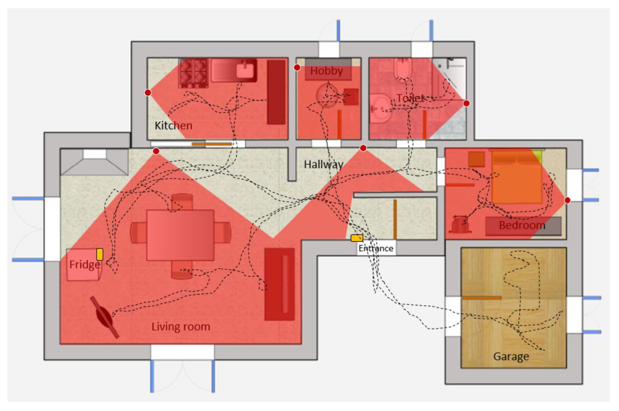
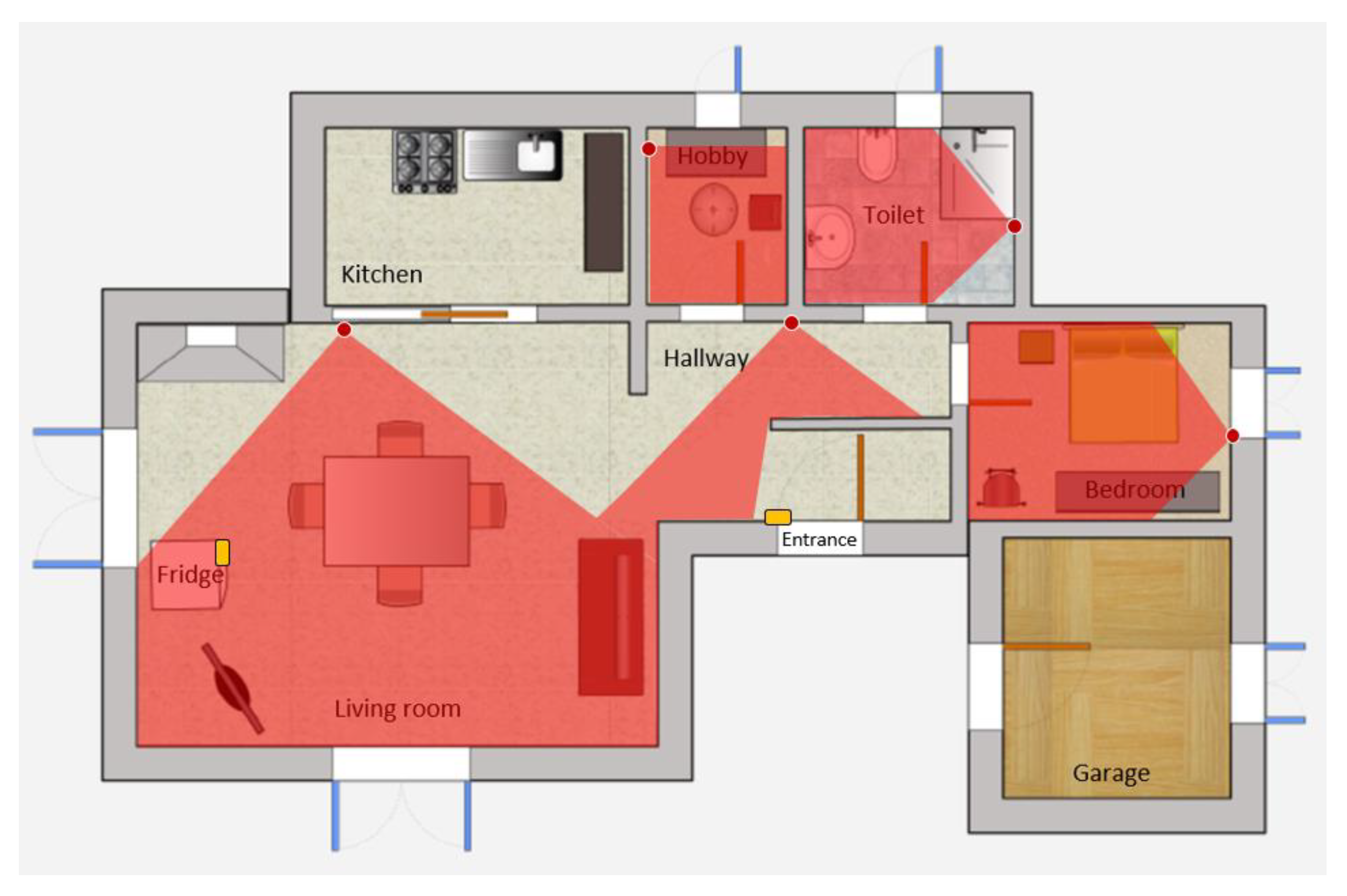
3.7. Case Study 1

The first SLE reported in this study is a seven-room apartment taken from the Italian pilot eWare. As a starting configuration, 5 PIR sensors were installed: one in the hallway, one in the bedroom, one in the toilet, one in the hobby room and one in the living room. Furthermore, 2 door sensors are installed: one on the fridge door and one on the entrance door, as in Figure 9.

The SLE tool offers a graphical representation of the simulated sensor activation data. Figure 10 shows, as an example, the graph of the 6 months of simulated data for the first home sensor network configuration of Case Study 1.

The second configuration, Figure 11, considers 6 PIR sensors, adding to the previous configuration one PIR sensor in the kitchen and removing the door sensor from the fridge.

The SLE tool also offers a statistical analysis area in which the time spent in each room (in seconds) and the number of sensor activations per room/door for the simulated datasets is reported. Figure 12 shows, as an example, the graphs related to the analysis of the 6 months of simulated data for the second home sensor network configuration of Case Study 1.

The third configuration, Figure 13, considers 5 PIR sensors and one door sensor on the entrance door, removing the previous configuration of the PIR sensor in the bedroom.

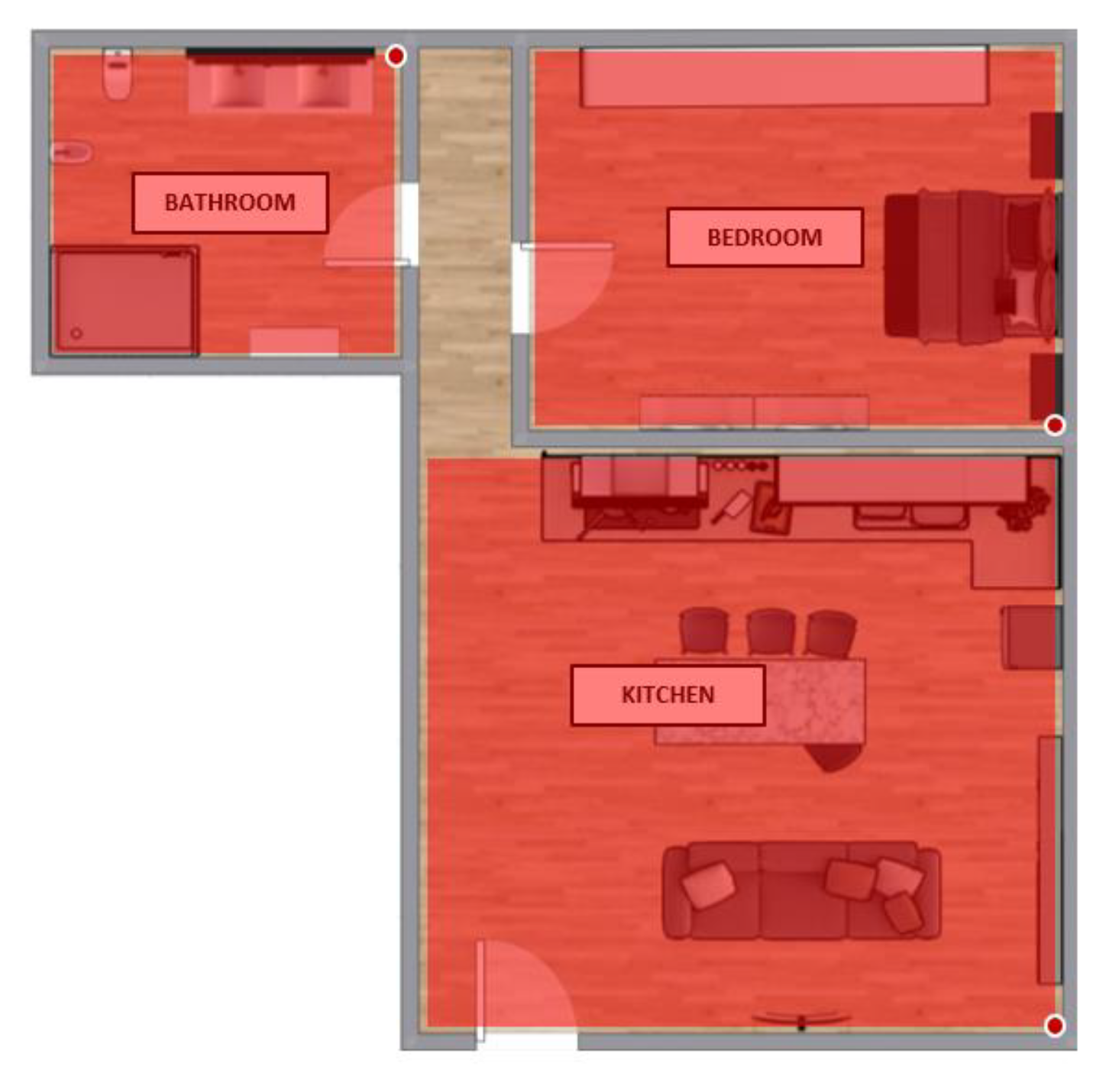
3.8. Case Study 2

The second SLE reported in this study is a small Japanese apartment with three rooms taken from the e-VITA project. As a starting configuration, 3 PIR sensors were installed: one in the toilet, one in the bedroom and one in the kitchen, Figure 14.

The second configuration, Figure 15, considers only 2 PIR sensors, removing from the previous configuration the PIR sensor in the bedroom.

The third configuration, Figure 16, adds to the second configuration a door sensor installed on the entrance door.

To summarize, the method proposed by the authors consists of the following steps:

-

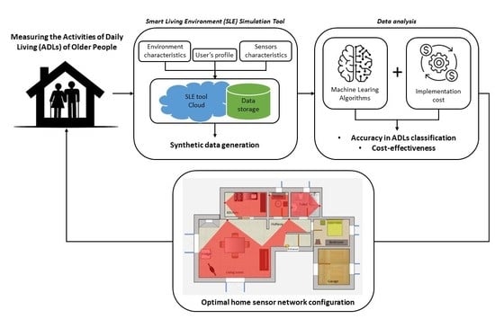
Identify which are the relevant ADLs to be measured for the older user.

-

Design different configurations of the home sensor network and recreate them in the SLE simulator.

-

Simulate the behaviour of the older user via the SLE tool to generate a consistent dataset of sensor activations.

-

Analyze the obtained dataset through ML algorithms and evaluate which configuration best measures the user’s ADLs (highest accuracy in ADLs classification).

-

Finally, the optimization of the home sensor network configuration is given by a cost-effectiveness analysis, in terms of ADL classification accuracy and the cost of the installed sensor network.

4. Results

This section presents the ML accuracy results in ADL classification for the different configurations of the home sensor network for the two case studies.

The results of the hold-out validation and 10-fold CV, considering as input the simulated 6 month datasets generated, are reported as values of the aforementioned evaluation metric. The performance of the four ML algorithms, considering the three different home sensor network configurations in the SLE of Case Study 1 for hold-out validation, is shown in

Table 2. Percentage values of precision, recall, F1-score and accuracy of the Decision Tree (DT), Support Vector Machine (SVM), K-Nearest Neighbors (KNN) and Gaussian Naïve Bayes (GNB) algorithms in classifying the user’s ADLs for hold-out validation for the three home sensor network configurations of Case Study 1.

Configurations	ML Algorithms	Precision [%]	Recall [%]	F1-Score [%]	Accuracy [%]
1	DT	98	98	98	98
	SVM	11	34	50	34
	KNN	85	81	82	81
	GNB	11	32	50	32
2	DT	99	99	99	99
	SVM	15	38	56	38
	KNN	58	76	87	76
	GNB	92	95	98	95
3	DT	98	98	98	98
	SVM	15	39	56	38
	KNN	36	52	45	52
	GNB	87	88	89	89

, while that for the 10-fold CV is shown in

Table 3. Mean percentage values over the splits of precision, recall, F1-score, and accuracy of the Decision Tree (DT), Support Vector Machine (SVM), K-Nearest Neighbors (KNN) and Gaussian Naïve Bayes (GNB) algorithms in classifying the user’s ADLs for a 10-fold CV for the three home sensor network configurations of Case Study 1.

Configurations	ML Algorithms	Precision [%]	Recall [%]	F1-Score [%]	Accuracy [%]
1	DT	94	90	90	99
	SVM	4	11	7	34
	KNN	70	69	66	94
	GNB	25	31	37	34
2	DT	99	99	99	99
	SVM	4	11	6	38
	KNN	70	70	69	93
	GNB	74	79	76	95
3	DT	99	99	99	99
	SVM	40	6	8	40
	KNN	80	80	79	97
	GNB	82	86	83	90

.

Table 4. Cost of the different home sensor network configurations of Case Study 1.

Configurations	Cost [GBP]
1	900
2	1000
3	850

instead shows the estimated cost of the different network configurations of Case Study 1.

The mean accuracies over the three home sensor network configurations of Case Study 1 achieved by the four ML algorithms for hold-out validation and 10-fold CV were computed to identify which of them was best-suited for classifying ADLs, as shown in Figure 17.

The performance of the four ML algorithms, considering the three different home sensor network configurations in the SLE of Case Study 2 for the hold-out validation is shown in

Table 5. Percentage values of precision, recall, F1-score and accuracy of the Decision Tree (DT), Support Vector Machine (SVM), K-Nearest Neighbors (KNN) and Gaussian Naïve Bayes (GNB) algorithms in classifying a user’s ADLs for hold-out validation for the three home sensor network configurations of Case Study 2.

Configurations	ML Algorithms	Precision [%]	Recall [%]	F1-Score [%]	Accuracy [%]
1	DT	98	98	98	98
	SVM	10	31	48	31
	KNN	45	64	81	64
	GNB	37	56	77	56
2	DT	91	91	91	91
	SVM	24	49	59	49
	KNN	79	80	79	80
	GNB	48	50	54	50
3	DT	93	94	94	94
	SVM	15	39	56	39
	KNN	46	65	81	65
	GNB	56	61	93	61

, while that for the 10-fold CV is shown in

Table 6. Mean percentage values over the splits of precision, recall, F1-score and accuracy of the Decision Tree (DT), Support Vector Machine (SVM), K-Nearest Neighbors (KNN) and Gaussian Naïve Bayes (GNB) algorithms in classifying a user’s ADLs for 10-fold CV for the three home sensor network configurations of Case Study 2.

Configurations	ML Algorithms	Precision [%]	Recall [%]	F1-Score [%]	Accuracy [%]
1	DT	94	94	94	97
	SVM	6	2	9	30
	KNN	56	56	53	63
	GNB	46	60	51	69
2	DT	93	91	92	91
	SVM	25	50	33	50
	KNN	60	75	83	80
	GNB	43	57	53	51
3	DT	83	82	81	94
	SVM	10	25	14	37
	KNN	71	70	68	82
	GNB	72	75	73	73

.

Table 7. Cost of the different home sensor network configurations of Case Study 2.

Configurations	Cost [GBP]
1	450
2	300
3	400

instead shows the estimated cost of the different network configurations of Case Study 2.

Figure 18 shows the mean accuracies over the three home sensor network configurations of Case Study 2 achieved by the four ML algorithms for hold-out validation, and 10-fold CVs were computed to identify which of them were best-suited for classifying ADLs.

5. Discussion

The authors assessed the accuracy of different home sensor network configurations in measuring specific ADLs using four different ML algorithms (i.e., DT, SVM, KNN, GNB). They decided to use different algorithms in order to compare their performance and determine which one would be most suitable to refer to during the optimization process of the home sensor network. Two SLE scenarios were recreated in the simulation tool: Case Study 1 using a real map of an apartment where an older user with a diagnosis of early-stage dementia involved in the Italian pilot eWare lived, and Case Study 2 using a map of a Japanese apartment taken from the e-VITA project. From the experience gained in the projects in which they were involved, the authors realized that in real scenarios, it is always difficult to design a correct configuration of PIR and door sensors to measure older people’s ADLs due to the different characteristics of users and apartments. Considering the scenarios used for this study, the authors identified that it was important for the older users to keep track of sleep patterns, eating activities (breakfast, lunch, dinner, cooking), personal hygiene activities (going to the toilet) and activities related to staying active and engaged in recreational activities (ambulating, dressing, entering/leaving, having a hobby, relaxing/watching TV). For each case study, three different home sensor network configurations were designed and 6 months of activity by an older virtual user were then simulated using the SLE tool, to generate datasets consisting of home sensor network activations.

The performances of the four ML algorithms tested on the generated datasets in terms of ADL classification accuracy, precision, F1-score and recall, considering the three different home sensor network configurations of Case Study 1 and Case Study 2 for hold-out validation are shown in Table 2 and Table 5, respectively. Each algorithm was trained on 70% of the generated 6-month datasets and tested on the remaining 30%. Table 3 and Table 6 show the mean values over the splits of ADL classification accuracy, precision, F1-score and recall of the ML algorithms for 10-fold CV considering the three home sensor network configurations of Case Study 1 and Case Study 2, respectively. Considering the measured accuracies as a comparison term, the results show that for Case Study 1 the DT classifier achieved the highest accuracy in classifying the user’s ADLs for both hold-out validation (98%) and 10-fold CV (99%). The mean accuracy achieved by the DT, KNN, SVM, GNB classifiers over the three home sensor network configurations of Case Study 1 (Figure 17) proved that the DT classifier is the most suitable in classifying ADLs with 98% mean accuracy for hold-out validation and 99% mean accuracy for 10-fold CV, compared to SVM (36% mean accuracy for hold-out validation and 37% mean accuracy for 10-fold CV), KNN (70% mean accuracy for hold-out validation and 94% mean accuracy for 10-fold CV), and GNB (72% mean accuracy for hold-out validation and 73% mean accuracy for 10-fold CV). The results for Case Study 2 also show that the DT classifier achieved the highest accuracy in classifying a user’s ADLs (over 91% for both hold-out validation and 10-fold CV). In fact, the mean accuracy over the three home sensor network configurations of Case Study 2 achieved by the ML algorithms (Figure 18) proved also in this case that the DT classifier is the most suitable in classifying ADLs with 94% mean accuracy for both hold-out validation and 10-fold CV, compared to SVM (39% mean accuracy for hold-out validation and 39% mean accuracy for 10-fold CV), KNN (70% mean accuracy for hold-out validation and 75% mean accuracy for 10-fold CV), and GNB (56% mean accuracy for hold-out validation and 60% mean accuracy for 10-fold CV). In the optimization process, therefore, the comparison between the sensor networks’ capabilities in the measurement of ADLs was carried out based on the accuracy achieved by the DT algorithm. In addition to being one of the most used supervised classification algorithms [35,36,37], DT requires no pre-processing actions and needs less time to process data than other algorithms. It provides a good forecast for datasets consisting of simple features, like our case, as opposed to SVM, which performs well on big and intricate datasets. Furthermore, as reported in [40,41], DT proves to be more accurate than KNN and GNB in classification problems. However, the problem of overfitting can affect such a ML classifier. There are specific techniques to mitigate it and one of them is to perform a k-fold CV on the dataset, which is also helpful in assessing the performance of ML models. In this study, the authors performed a 10-fold CV on the dataset, which means that the ML algorithms divided the data into 10 parts to execute the adaptation process 10 times, with each adaptation executed on a training set of 90% of the total randomly chosen training sets, whereas the remaining 10% served validation purposes.

In the process of optimizing the sensor network installed in the user’s home, with the aim of minimizing the number of sensors and installing them in optimal locations without losing measurement accuracy, the cost of the technology and user acceptance must be considered. Table 4 and Table 7 show the cost of the home sensor network for the different configurations for the two case studies considering a cost of GBP 150 for each Delta Dore DMB Tyxal + PIR sensor and GBP 100 for each Delta Dore DO BL Tyxal + door sensor, which are the sensors modeled in the simulation resulting from the experience of use in the e-VITA project. To ensure greater acceptability by older people, it is thus recommended to reduce the number of sensors to be installed in the home. By optimizing the home sensor network configuration and relating costs to the effectiveness of the configuration, the behaviour of older people can be monitored with high accuracy while minimizing the installation costs. Considering, for example, the three configurations in Case Study 1, all of them provide high accuracy in measuring older users’ ADLs, so it is appropriate to use the least expensive one that will still have a high impact on user monitoring while lowering costs. Optimizing the home sensor network consequently improves the process of remote monitoring of older people, enabling the deployment of cost-effective and prompt healthcare services, such as early detection of patient decline. This contributes to reducing the workload for hospitals, preventing frequent visits, and allowing the older person to age safely at home. Looking at the trend (orange line in Figure 19) of the ML accuracy and the number of sensors, by using a few sensors, the accuracy in classifying ADLs is still high (over 90%) while keeping costs low (blue line in Figure 19). Therefore, taking into account the minimization of the number of sensors and costs while guaranteeing high measurement accuracy, the optimal configuration of the home sensor network for Case Study 1 is the third that, with a total cost of GBP 850, allows to achieve over 98% accuracy in ADLs classification using the DT algorithm, while for Case Study 2 it is the second that, with a cost of GBP 300, allows to achieve 91% accuracy using the DT algorithm.

Finally, based on the experience gained in the study and previous projects, the following recommendations can be given on sensor installation. The PIR and door sensors should be installed in the relevant areas within the house, determined by predefined ADLs to be measured according to the use case. It is preferable to install PIR sensors at a minimum height of 1.4 m above the ground to better detect movements and to cover the whole area of interest. It is better not to overlap the detection areas of two or more sensors to avoid false detections, and it is preferable to avoid installing them near objects that obscure their field of view.

6. Conclusions

The main contribution of this work is the presentation of a methodology to optimize the home sensor network to measure the ADLs of older people using ML applied to synthetic data generated via a newly developed SLE simulation tool.

From the experience gained by the authors in previous projects, the need emerged to establish a methodology to identify a priori the optimal configuration of the sensor network to measure the behaviour of older users. A system architect must in fact choose the right approach to design the home sensor network, verifying whether additional sensors or different positions would improve or impair the desired result. At this stage, test data are required to verify whether the designed sensor network ensures the necessary accuracy in measuring ADLs. To speed up the data generation process and overcome the problems of reproducing the sensor network in the laboratory to generate real datasets, the authors developed a SLE simulation tool for simulating human activities, and thus sensor activations, in the reconstructed environment, based on the hybrid approach described by Al-Shammari et al. [21]. The SLE simulation tool was designed to avoid the use of time-consuming processes such as the use of the 3D Blender tool required by OpenSHS to design the environment and the installed sensors. Unlike the latter, in fact, the developed simulator simply requires the loading of the 2D map to reproduce the home environment, considerably speeding up the process. Another advantage over the simulators in the literature is that a large amount of PIR and door sensor activation data can be generated from a single day of simulated virtual user trajectories thanks to an automatic random perturbation system. The authors proved that by analyzing the accuracy of users’ ADL classification using the DT algorithm, the home sensor network configuration can be modified to provide the most suitable design for the use case. The advantage of this method is that an inadequate sensor network design may be identified in an earlier phase of development and cost-effectiveness estimates can be made beforehand, identifying the optimal trade-off of sensor numbers, implementation costs, and accuracy in measuring older people’s ADLs.

References

- Andò, B.; Baglio, S.; Castorina, S.; Crispino, R.; Marletta, V. Advanced Sensing Solutions for Ambient Assisted Living: The NATIFLife Framework. IEEE Instrum. Meas. Mag. 2020, 23, 33–40. [Google Scholar] [CrossRef]
- Casaccia, S.; Romeo, L.; Calvaresi, A.; Morresi, N.; Monteriù, A.; Frontoni, E.; Scalise, L.; Revel, G.M. Measurement of Users’ Well-Being Through Domotic Sensors and Machine Learning Algorithms. IEEE Sens. J. 2020, 20, 8029–8038. [Google Scholar] [CrossRef]
- Naccarelli, R.; Casaccia, S.; Revel, G. The Problem of Monitoring Activities of Older People in Multi-Resident Scenarios: An Innovative and Non-Invasive Measurement System Based on Wearables and PIR Sensors. Sensors 2022, 22, 3472. [Google Scholar] [CrossRef] [PubMed]
- Pietroni, F.; Casaccia, S.; Revel, G.M.; Scalise, L. Methodologies for Continuous Activity Classification of User through Wearable Devices: Feasibility and Preliminary Investigation. In Proceedings of the 2016 IEEE Sensors Applications Symposium (SAS), Catania, Italy, 20–22 April 2016; pp. 1–6. [Google Scholar]
- Casaccia, S.; Naccarelli, R.; Moccia, S.; Migliorelli, L.; Frontoni, E.; Revel, G.M. Development of a Measurement Setup to Detect the Level of Physical Activity and Social Distancing of Ageing People in a Social Garden during COVID-19 Pandemic. Measurement 2021, 184, 109946. [Google Scholar] [CrossRef]
- Ooi, B.Y.; Beh, W.L.; Lee, W.; Shirmohammadi, S. Using the Cloud to Improve Sensor Availability and Reliability in Remote Monitoring. IEEE Trans. Instrum. Meas. 2019, 68, 1522–1532. [Google Scholar] [CrossRef]
- Massaroni, C.; Nicolò, A.; Schena, E.; Sacchetti, M. Remote Respiratory Monitoring in the Time of COVID-19. Front. Physiol. 2020, 11, 635. [Google Scholar] [CrossRef]
- Chen, Z.; Wang, Y.; Liu, H. Unobtrusive Sensor-Based Occupancy Facing Direction Detection and Tracking Using Advanced Machine Learning Algorithms. IEEE Sens. J. 2018, 18, 6360–6368. [Google Scholar] [CrossRef]
- Sprint, G.L.; Cook, D.J.; Fritz, R. Behavioral Differences Between Subject Groups Identified Using Smart Homes and Change Point Detection. IEEE J. Biomed. Health Inform. 2020, 25, 559–567. [Google Scholar] [CrossRef]
- De, P.; Chatterjee, A.; Rakshit, A. PIR Sensor Based AAL Tool for Human Movement Detection: Modified MCP Based Dictionary Learning Approach. IEEE Trans. Instrum. Meas. 2020, 69, 7377–7385. [Google Scholar] [CrossRef]
- Chowdhury, D.; Chattopadhyay, M. Development of a Low Power Microcontroller Based Wrist-Worn Device with Resource Constrained Activity Detection Algorithm. IEEE Trans. Instrum. Meas. 2020, 69, 7522–7529. [Google Scholar] [CrossRef]
- Xing, Y.; Wang, T.; Zhou, F.; Hu, A.; Li, G.; Peng, L. EVAL Cane: Non-Intrusive Monitoring Platform with a Novel Gait-Based User Identification Scheme. IEEE Trans. Instrum. Meas. 2020, 70, 1–15. [Google Scholar] [CrossRef]
- Gochoo, M.; Tan, T.; Liu, S.; Jean, F.; Alnajjar, F.; Huang, S. Unobtrusive Activity Recognition of Elderly People Living Alone Using Anonymous Binary Sensors and DCNN. IEEE J. Biomed. Health Inform. 2018, 23, 693–702. [Google Scholar] [CrossRef] [PubMed]
- Mora, N.; Grossi, F.; Russo, D.; Barsocchi, P.; Hu, R.; Brunschwiler, T.; Michel, B.; Cocchi, F.; Montanari, E.; Nunziata, S.; et al. IoT-Based Home Monitoring: Supporting Practitioners’ Assessment by Behavioral Analysis. Sensors 2019, 19, 3238. [Google Scholar] [CrossRef] [PubMed] [Green Version]
- Piau, A.; Lepage, B.; Bernon, C.; Gleizes, M.-P.; Nourhashemi, F. Real-Time Detection of Behavioral Anomalies of Older People Using Artificial Intelligence (The 3-PEGASE Study): Protocol for a Real-Life Prospective Trial. JMIR Res. Protoc. 2019, 8, e14245. [Google Scholar] [CrossRef]
- Shirali, M.; Bayo Montón, J.; Fernandez-Llatas, C.; Ghassemian, M.; Traver, V. Design and Evaluation of a Solo-Resident Smart Home Testbed for Mobility Pattern Monitoring and Behavioural Assessment. Sensors 2020, 20, 7167. [Google Scholar] [CrossRef]
- Doyle, J.; Kealy, A.; Loane, J.; Walsh, L.; O’Mullane, B.; Flynn, C.; Macfarlane, A.; Bortz, B.; Knapp, R.B.; Bond, R. An Integrated Home-Based Self-Management System to Support the Wellbeing of Older Adults. J. Ambient Intell. Smart Environ. 2014, 6, 359–383. [Google Scholar] [CrossRef] [Green Version]
- Eisa, S.; Moreira, A. A Behaviour Monitoring System (BMS) for Ambient Assisted Living. Sensors 2017, 17, 1946. [Google Scholar] [CrossRef] [Green Version]
- Casaccia, S.; Revel, G.M.; Scalise, L.; Bevilacqua, R.; Rossi, L.; Paauwe, R.A.; Karkowsky, I.; Ercoli, I.; Artur Serrano, J.; Suijkerbuijk, S.; et al. Social Robot and Sensor Network in Support of Activity of Daily Living for People with Dementia. In Proceedings of the Dementia Lab 2019. Making Design Work: Engaging with Dementia in Context, Eindhoven, The Netherlands, 21–22 October 2019; Brankaert, R., IJsselsteijn, W., Eds.; Springer International Publishing: Cham, Switzerland, 2019; pp. 128–135. [Google Scholar]
- Casaccia, S.; Jokinen, K.; Naccarelli, R.; Revel, G.M. Well-Being and Comfort of Ageing People Based on Indoor Environmental Conditions: Preliminary Study on Human-Coach Conversation. In Proceedings of the 2022 IEEE International Workshop on Metrology for Living Environment (MetroLivEn), Cosenza, Italy, 25–27 May 2022; pp. 164–169. [Google Scholar]
- Alshammari, N.; Alshammari, T.; Sedky, M.; Champion, J.; Bauer, C. OpenSHS: Open Smart Home Simulator. Sensors 2017, 17, 1003. [Google Scholar] [CrossRef] [Green Version]
- Synnott, J.; Nugent, C.; Jeffers, P. Simulation of Smart Home Activity Datasets. Sensors 2015, 15, 14162–14179. [Google Scholar] [CrossRef]
- Renoux, J.; Klugl, F. Simulating daily activities in a smart home for data generation. In Proceedings of the 2018 Winter Simulation Conference (WSC), Gothenburg, Sweden, 9–12 December 2018; pp. 798–809. [Google Scholar]
- Buchmayr, M.; Kurschl, W.; Küng, J. A Simulator for Generating and Visualizing Sensor Data for Ambient Intelligence Environments. Procedia Comput. Sci. 2011, 5, 90–97. [Google Scholar] [CrossRef]
- Helal, S.; Lee, J.W.; Hossain, S.; Kim, E.; Hagras, H.; Cook, D. Persim—Simulator for Human Activities in Pervasive Spaces. In Proceedings of the 2011 Seventh International Conference on Intelligent Environments, Nottingham, UK, 25–28 July 2011; pp. 192–199. [Google Scholar]
- Kormányos, B.; Pataki, B. Multilevel Simulation of Daily Activities: Why and How? In Proceedings of the 2013 IEEE International Conference on Computational Intelligence and Virtual Environments for Measurement Systems and Applications (CIVEMSA), Milan, Italy, 13–17 July 2013; pp. 1–6. [Google Scholar]
- Bouchard, K.; Ajroud, A.; Bouchard, B.; Bouzouane, A. SIMACT: A 3D Open Source Smart Home Simulator for Activity Recognition with Open Database and Visual Editor. Int. J. Hybrid Inf. Technol. (IJHIT) 2012, 5, 13–32. [Google Scholar]
- Park, J.; Moon, M.; Hwang, S.; Yeom, K. CASS: A Context-Aware Simulation System for Smart Home. In Proceedings of the 5th ACIS International Conference on Software Engineering Research, Management & Applications (SERA 2007), Washington, DC, USA, 20–22 August 2007; pp. 461–467. [Google Scholar]
- Caruso, M.; Ilban, Ç.; Leotta, F.; Mecella, M.; Vassos, S. Synthesizing Daily Life Logs through Gaming and Simulation. In Proceedings of the 2013 ACM Conference on Pervasive and Ubiquitous Computing Adjunct Publication, Zurich, Switzerland, 8–12 September 2013; Association for Computing Machinery: New York, NY, USA, 2013; pp. 451–460. [Google Scholar]
- Synnott, J.; Chen, L.; Nugent, C.D.; Moore, G. The Creation of Simulated Activity Datasets Using a Graphical Intelligent Environment Simulation Tool. In Proceedings of the 2014 36th Annual International Conference of the IEEE Engineering in Medicine and Biology Society, Chicago, IL, USA, 26–30 August 2014; pp. 4143–4146. [Google Scholar]
- Ariani, A.; Redmond, S.J.; Chang, D.; Lovell, N.H. Simulation of a Smart Home Environment. In Proceedings of the 2013 3rd International Conference on Instrumentation, Communications, Information Technology and Biomedical Engineering (ICICI-BME), Bandung, Indonesia, 7–8 November 2013; pp. 27–32. [Google Scholar]
- Nishikawa, H.; Yamamoto, S.; Tamai, M.; Nishigaki, K.; Kitani, T.; Shibata, N.; Yasumoto, K.; Ito, M. UbiREAL: Realistic Smartspace Simulator for Systematic Testing. In Proceedings of the UbiComp 2006: Ubiquitous Computing, Orange County, CA, USA, 17–21 September 2006; Dourish, P., Friday, A., Eds.; Springer: Berlin/Heidelberg, Germany, 2006; pp. 459–476. [Google Scholar]
- Casaccia, S.; Rosati, R.; Scalise, L.; Revel, G.M. Measurement of Activities of Daily Living: A Simulation Tool for the Optimisation of a Passive Infrared Sensor Network in a Smart Home Environment. In Proceedings of the 2020 IEEE International Instrumentation and Measurement Technology Conference (I2MTC), Dubrovnik, Croatia, 25–28 May 2020; pp. 1–6. [Google Scholar]
- Pirozzi, M. Development of a Simulation Tool for Measurements and Analysis of Simulated and Real Data to Identify ADLs and Behavioral Trends through Statistics Techniques and ML Algorithms. Ph.D. Thesis, Univeristà Politecnica delle Marche, Ancona, Italy, 2020. [Google Scholar]
- Atallah, L.; Lo, B.; Ali, R.; King, R.; Yang, G.-Z. Real-Time Activity Classification Using Ambient and Wearable Sensors. IEEE Trans. Inf. Technol. Biomed. 2009, 13, 1031–1039. [Google Scholar] [CrossRef] [PubMed]
- Ariani, A.; Redmond, S.J.; Chang, D.; Lovell, N.H. Software Simulation of Unobtrusive Falls Detection at Night-Time Using Passive Infrared and Pressure Mat Sensors. In Proceedings of the 2010 Annual International Conference of the IEEE Engineering in Medicine and Biology, Buenos Aires, Argentina, 31 August–4 September 2010; pp. 2115–2118. [Google Scholar]
- Hu, Y.-J.; Yu, M.-C.; Wang, H.-A.; Ting, Z.-Y. A Similarity-Based Learning Algorithm Using Distance Transformation. IEEE Trans. Knowl. Data Eng. 2015, 27, 1452–1464. [Google Scholar] [CrossRef]
- Francillette, Y.; Bouchard, B.; Bouchard, K.; Gaboury, S. Modeling, Learning, and Simulating Human Activities of Daily Living with Behavior Trees. Knowl. Inf. Syst. 2020, 62, 3881–3910. [Google Scholar] [CrossRef]
- Roy, P.C.; Bouchard, B.; Bouzouane, A.; Giroux, S. Ambient Activity Recognition in Smart Environments for Cognitive Assistance. Available online: www.igi-global.com/article/ambient-activity-recognition-in-smart-environments-for-cognitive-assistance/95226 (accessed on 1 October 2020).
- Mohanapriya, M.; Lekha, J. Comparative Study between Decision Tree and Knn of Data Mining Classification Technique. J. Phys. Conf. Ser. 2018, 1142, 012011. [Google Scholar] [CrossRef]
- Rahmadani, S.; Dongoran, A.; Zarlis, M.; Zakarias. Comparison of Naive Bayes and Decision Tree on Feature Selection Using Genetic Algorithm for Classification Problem. J. Phys. Conf. Ser. 2018, 978, 012087. [Google Scholar] [CrossRef]