Article

An Experimental and Numerical Study on Fire Spread in a Furnished Room

by
Małgorzata Król
1,* and
Aleksander Król
2
1
Faculty of Energy and Environmental Engineering, Silesian University of Technology, Konarskiego 18, 44-100 Gliwice, Poland
2
Faculty of Transport and Aviation Engineering, Silesian University of Technology, Krasińskiego 8, 40-019 Katowice, Poland
*
Author to whom correspondence should be addressed.
Buildings 2022, 12(12), 2189; https://doi.org/10.3390/buildings12122189
Submission received: 4 November 2022 / Revised: 6 December 2022 / Accepted: 8 December 2022 / Published: 10 December 2022
(This article belongs to the Special Issue Building Physics, Structural and Safety Engineering)

Abstract

:
The main objective of this research was to examine the development of fire in a furnished room in a typical high-rise building. This work was part of research on the fire safety of building occupants. It included two controlled fires in which a standard sofa in a room was set on fire. Several thermocouple trees were arranged in the test room and the temperature was continuously recorded. Additionally, each fire test was videotaped for further analysis. Since an unexpected forepeak of the temperature course was observed, special attention was paid to explain this phenomenon. For this purpose, numerical models of fire development in a furnished room were built using the well-recognized software package, ANSYS Fluent and Fire Dynamic Simulator (FDS). The numerical research was focused on fire spread over a single piece of furniture, the sofa. The data recorded in real experiments were used to tune and validate the numerical models. The results of the Fluent numerical simulation were consistent with the recorded experimental data and proved that after the initial growth, there was a critical phase of fire development in which the fire might almost snuff or flare again. Meanwhile, the FDS results, despite being generally in accordance with the experiment, did not reproduce this critical phase of fire spreading.

1. Introduction

The development of a fire in an enclosed space poses a huge risk to anyone within. Engineers are constantly working to improve the safety of people in buildings [1,2,3,4]. This relates to the development of nonflammable materials and the continuous improvement of fire ventilation and extinguishing systems. It also applies to the location of combustible materials in the vicinity of particularly tall buildings [5]. There is also ongoing research on the proper modeling of the fire development phenomenon to reliably reproduce air and smoke flows and structural fire resistance [6]. The fire risk index for buildings was also created to define the level of fire threat in buildings [7].
When considering a fire developing in a compartment, it should be remembered that its course is determined by the availability of air and fuel. One commonly uses the terms that the fire is controlled by fuel supply (fuel limited) or air supply (oxygen limited) [8]. In the literature, the terms Regime I and Regime II, respectively [9], can also be found. Regime I is characterized by the vents being small enough that they allow for the compartment to fill with smoke. The air supply is limited. In Regime II, the vents are sufficiently large, so that the smoke evacuates the enclosure and the air flows inside. Complex heat and mass transfer processes dominate over Regime II [10]. This makes the description of Regime II complicated, and it is difficult to define the direct link between ventilation, temperature and burning rate, as it can be done for Regime I.
Numerical analyses are increasingly used in all these activities, but some difficulties arise when connecting these analyses with tests and trials under real fire conditions. However, numerical analyses seem to be a good tool for testing various types of fire engineering solutions. However, it should be noted that the numerical models created during such analyses must be validated using real fires.
Research involving the mapping of fire development using fire zone model [11] computational fluid dynamics (CFD) programs has been carried out for many years [10,12,13]. The Fire Dynamics Simulator (FDS) is often used in these analyses. Analysis of the research conducted so far shows that modeling fire development in rooms faces many problems. The large number of parameters determining the course of such a fire makes it difficult to represent a fire numerically.
Modeling the temperature distribution in a room where a fire develops is difficult. Stern-Gottfried points out that the temperature distribution in a room is not uniform. Locally, the maximum temperature can be 75% higher than the average temperature for a given room [14]. The Dalmarnock Fire Test One was used for their analyses. The same studies were also used to validate the numerical model developed in the Fire Dynamics Simulator (FDS). Extensive measurements allowed for an analysis of the measured results against the results of numerical analyses. As part of the study, the authors noted the difficulty of modeling near the fire and the relatively good agreement of the results away from the fire [15].
Research on fires developing in confined spaces also concerns the impact of fire on the building structure. Gupta studied the thermal characteristics of fire spread in a fully developed fire, a growing fire, and a traveling fire. This was possible because, unlike the previous research, Gupta conducted his research in a very large open plan compartment. According to their research, each fire spread mode induced significant and characteristic spatial heat distributions [16].
Research on the development of fires in confined spaces often includes studies on the development of flames outside openings on the façade of a building. These studies are important to understand the causes and course of a fire that develops along the façade of the building [17,18,19]. The windows on the façade of a building can cause the flames to spread outside the room onto the façade [20,21]. However, windows can also affect the course of a fire inside the room. This is related to the intense air inflow into the room forced by a fire plume. The effect of incoming air into a building due to wind is particularly evident in the case of a tall building fire [22], but it can also be used to create good conditions on the refuge floor [23]. Airflow can disturb the natural stratification in the room and cause hot smoke to mix with cold air. This can result in the disappearance of the hot and cooler layers [24]. This research not only concerns windows on the building façade, it also includes investigations of doors fitted with an air curtain. Research has been conducted on how the effect of an air curtain jet influences the temperature in the upper layer of a compartment fire [25].
Experimental investigations and numerical simulations of small room fires have already been performed in the literature [26]. Chen performed the measurements in a room built in a laboratory, which allowed them to monitor multiple parameters during the development of a fire. However, the conditions of the experiment were significantly different from those of a real fire. The measurements were compared with the results of numerical analyses in which the Fire Dynamic Simulator was used. The results were highly comparable. Material properties and oxygen limit settings in the FDS software were tested to explore their influence on the tendency of heat release rate. A.H. Majdalani carried out similar research on the development of fires. He built a room model in the laboratory and examined the principal characteristics of two unique behaviors of a fully developed compartment fire. Experimentation and computational modeling were used to explore, compare and contrast the characteristics of these two behaviors [27].
Research has also been conducted on the development of fires in real buildings. The experiment was carried out in a warehouse building, where a fire was planned on a shelf on a rack. The ignition, fire spread and combustion characteristics were studied. At the same time, CFD analyses were performed with the use of FDS. The results demonstrated a high degree of agreement between the experimental results and the CFD data. However, attention was drawn to the limited possibilities of modeling using FDS [28].
Similarly, Bystrom described interesting studies. They performed a fire experiment in a concrete building at a low ambient temperature. Research has shown that a compartment can be divided into two layers during a fire. However, the temperature in the upper layer is not uniform. The differences in temperature values were related to the distance from the fire source. A series of numerical analyses using FDS were also performed, and the outside temperature was assumed. The study demonstrated that the power of a fire would be greater at a higher outside temperature [29].
Mackay described compartment fire behavior training combined with numerical analyses using FDS. The main objective of the research was the training of firefighters. The results of these studies were also used to validate the numerical model [30]. In addition to the FDS program, the CFX program was used in the numerical analyses of the development of compartment fires. Hasib used the results of an experimental fire generated in an enclosure during the growth period to validate the predictions of CFX [31]. Fire studies conducted in the compartment are sometimes limited to the analysis of flame spread over solid fuels. He led the research, the main goal of which was to compare the surface and internal heat transfers to understand the mechanism underlying the degree of fuel packing [32,33]. Another study looked at the heat and mass transport process that defines the dynamics of combustion and flame spread in the case of wood crib fires in large rooms [34].
In the present study, fire tests were carried out in a room, which was enclosed in panels with high fire resistance. Six thermocouple trees were placed inside the room to measure the temperature during the tests. Additionally, the fire tests were recorded on video. The work is based mainly on the temperature distributions recorded in two fire tests which differed in the moment when the firefighting operation began. When analyzing the time dependence of the temperature, an unexpected course of the fire development was revealed: a clear forepeak was observed for almost all temperature curves. Therefore, numerical models were built to investigate this phenomenon. The well-recognized general purpose software packages Ansys Fluent and FDS were used. This former choice was justified by the possibility of a detailed investigation of model interdependencies at a very basic level [35]; the latter one is commonly used in fire engineering. In addition, the use of two software packages made it possible to compare the results achieved by them and their capabilities. The problems encountered when performing numerical analyses are presented in the manuscript, along with solutions that can help other researchers with numerical modeling of fire development in a room.

2. Materials and Methods

The main aim of the research was to test different configurations of a staircase smoke removal system, which is a crucial aspect of safe evacuation in high-rise buildings. The system consisted of an air supply fan with adjustable capacity and roof discharging vents, among others. In addition to these analyses, the test room was equipped with measurement devices, which allowed for the detailed analyses of compartment fire development. The experiments required the permanent presence of a fire brigade to ensure the appropriate safety level for the staff and material assets.
The test room was prepared on the 5th floor of a 9-story abandoned office building (Figure 1). The room was connected to the staircase through a short corridor with a remotely controlled door.

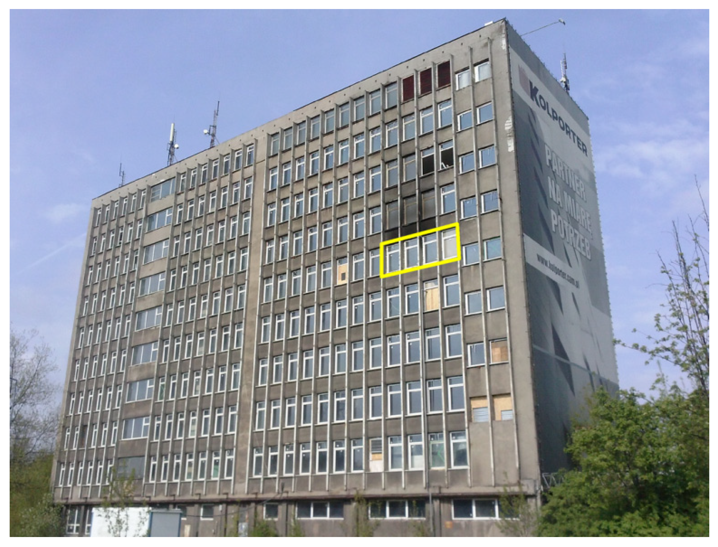
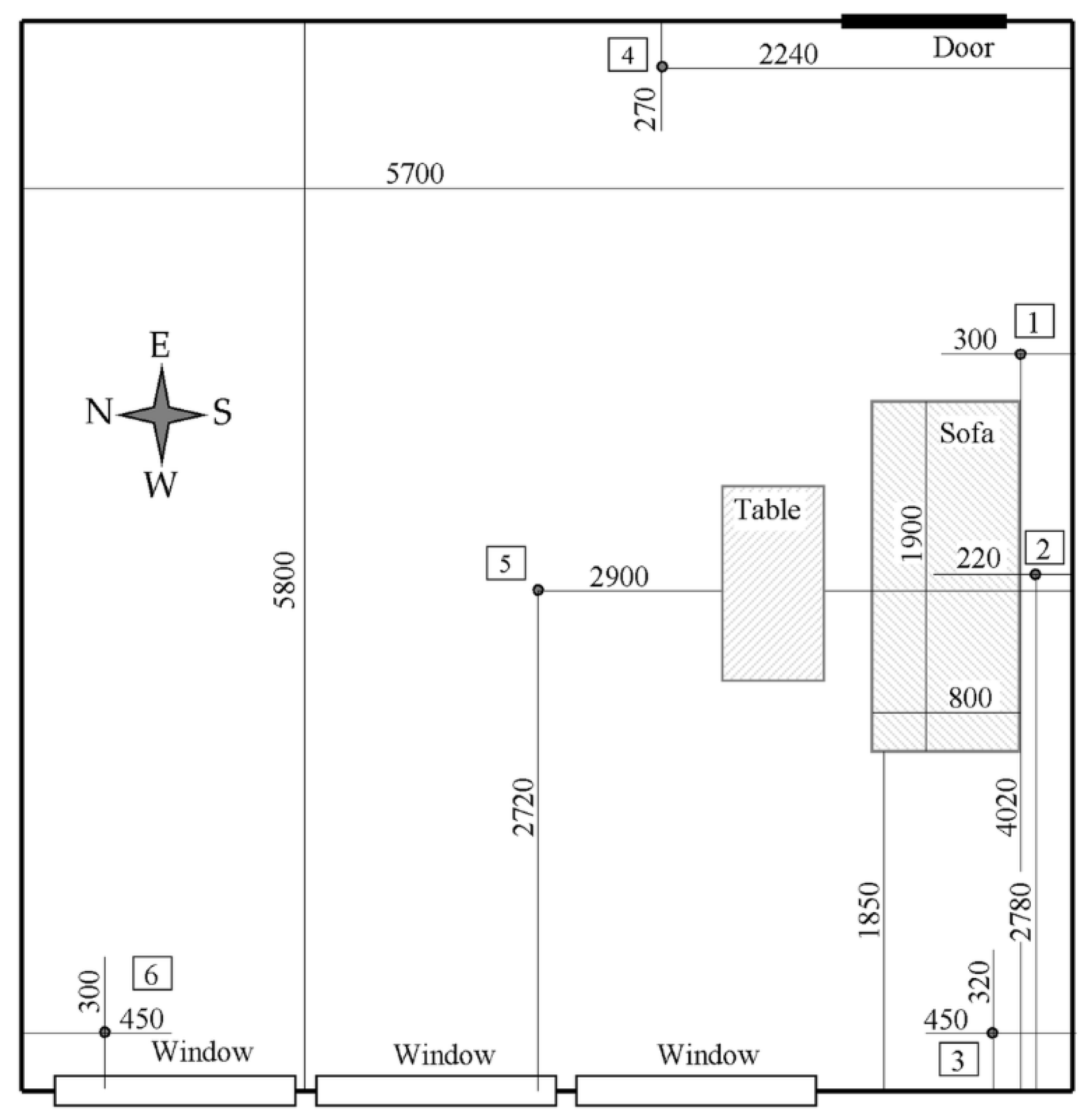
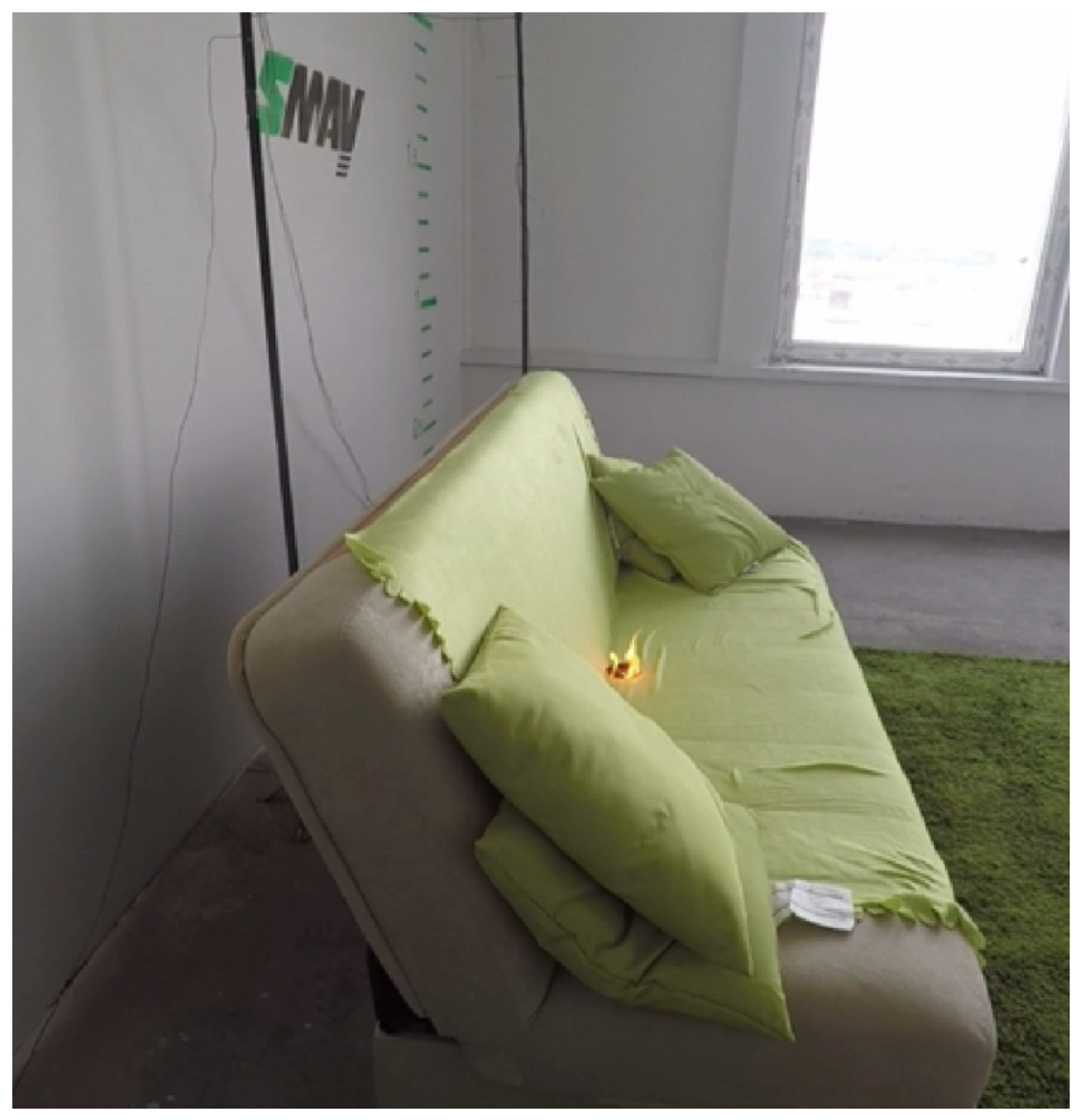
2.1. Experimental Setup

The test room was 5.7 × 5.8 × 2.5 m and had four windows. The rightmost window was built up with a cover from the inside. The three other glassed windows were tight. There was a door on the opposite side of the room from the windows. During both tests, the door connecting the test room to the corridor was open. Room partitions were covered with fireproof boards. The fireproof boards were made of silicate cement with a thickness of 50 mm and the following parameters: density 450 kg/m3, specific heat 950 J/kg∙K and thermal conductivity 0.083 W/m∙K. There was a sofa and a table in the room. The furniture was the same in each test.
Six thermocouple trees were distributed throughout the test room, as shown in the figure (Figure 2). There were three to eight thermocouples in the individual trees. K-type thermocouples with beads of 3 mm diameter were used. The sheath was made of heat resistant steel and was insulated inside with magnesium oxide. The measurement accuracy for the thermocouples was ±2.2 °C or 0.75% in the range of 0–1200 °C. The NI-9213 Temperature Input Modules recorded temperature measurements [36]. Signal Express National Instruments software was used for data acquisition. The positions of the thermocouples in individual trees are shown in Table 1.
The ignition source no. 4 from BS 5852:2006 was used to start the fires [37]. This standard ignition source is described in detail by Gupta [34]. The parameters of the ignition source are as follows: bar length 40 mm, bar width 6.5 mm, number of bars 10, bar weight 8.5 g, number of bar layers in two directions 5, and sterile gauze dimensions 40 × 40 mm. 1.4 mL of isopropyl alcohol was applied to the sterile gauze before starting the test. The igniter was placed in the middle of the sofa, as shown in Figure 3.

2.2. Experiment Results

Two full-scale fires were performed in the test room. The meteorological conditions during both fire tests are presented in Table 2.
The beginning of the fire was similar in both tests. The temperature inside the room was 17 °C, and the ignition source successfully initiated the fire development. First, the sofa backrest lit up. Then the flame grew larger and larger forming a conical burning region at the backrest. Next, the room was gradually filled with smoke and hot combustion gases and the fire still developed until it covered the entire sofa. This can be seen in a series of images presented in Figure 4.
During the first test, as shown in Table 2, the outside temperature was significantly higher, but should not have impacted on the conditions inside the room significantly. However, it was observed (Figure 5 and Figure 6) that the temperature above the sofa started to rise almost three minutes earlier than in the second test fire. This was probably caused by different storage conditions of the sofa prior to the experiment, such as packaging methods and room humidity. The first phase of the fire, which did not change the temperature above the sofa, lasted about seven minutes. Then, the temperature started to increase and, in the tenth minute, the temperature above the back of the sofa (at 1.6 m) reached 600 °C. Then, it dropped and started to rise again, reaching 800 °C. At that moment, the decision was made to start the firefighting operation. The entire set of temperature distributions is presented in Figure 5.
In the temperature distribution charts for individual thermocouple trees, it is clear that the highest temperature was achieved on the second and third trees. This suggests that smoke and hot air accumulated above the sofa and in the corner of the room by the window. Cold air flowing through the open door probably caused the temperatures on the first thermocouple tree to be lower. The temperatures further down the room, at some distance from the source of the fire, were also lower. In the case of the fifth and sixth trees, the temperature did not reach 600 °C. The course of temperature variation was the same in all trees. The graphs appear to show the stratification of air in the room, which manifested in lower temperatures at low heights, and high temperatures were almost the same at the higher points. This is especially visible for thermocouple trees away from the sofa (trees 5 and 6).
After the first test, the room was cleaned and returned to its original state. This included replacing windows because they may have been weakened due to the heat. During the second fire test, the first phase of the fire lasted almost ten minutes. Then, the flames spread rapidly in two minutes. Above the back of the sofa (at 1.6 m), the temperature increased to 700 °C. Next, the temperature dropped and then started to rise again. So, the odd course of fire spread was observed again; there were moments when the fire dimmed slightly. Eventually, the temperature reached over 1100 °C in the twentieth minute. Such a high temperature caused the windows to fall out, resulting in a rapid temperature drop. The diagrams of the temperature distribution during the second fire test for all thermocouple trees are shown in Figure 6. Five minutes after the windows had fallen out, the firefighting operation began, as shown in Figure 7. As can be seen, the room reached flashover and the flames were ejected from the window openings. This was confirmed during the room inspection, after the fire was completely extinguished—all equipment items were completely burnt.
When examining the temperature data, it is clear that until the maximum temperature is reached, the shapes of the curves are similar to those of the first fire. After the initial period of growth, there is a decrease and then an increase to the maximum values. Once the maximum temperature is reached for all measuring points, the temperature drops. However, in the second fire test, it is not caused by the intentional extinguishing action, but by the windows’ disintegration and the cold air inflow. As a result, the temperature did not drop in the same way as in the first fire. Instead, the temperature dropped slowly after the windows fell out, and the test room cooled down freely until the extinguishing action began.
As was mentioned earlier, the fire developed slower in the second fire test; this is also visible when comparing the time between the first increase of temperature to the forepeak. This was analyzed for the thermocouple tree no. 2: the temperature at the forepeak is almost the same in both tests (650–700 °C), but the time was 115 s in the first test and 140 s in the second one. Similarly, the time between the forepeak and the moment when 800 °C was reached is shorter in the first test (170 s vs. 281 s). These differences occurred despite the same experimental setup in both tests.
In both fire tests, a significant nonuniformity of the temperature distribution was observed, which could be expected because only the growth phase was examined. Two groups of thermocouple trees are notable: the first group contains trees located just close to the fire source (1 and 2) and the tree in the near corner (3), where the hot gases accumulated. The second group consists of distant trees (4 and 6) and the tree in the middle of the room (5), where the free spread of hot gases occurred. It was particularly visible in the fire growth phase: the measured temperature was almost independent of the height for the first group. Meanwhile, the temperature recorded by the second group indicated a clear stratification. This stratification almost ceased for the developed fire, excluding tree 6. Although, even for the developed fire, the maximum recorded temperature was distributed very unevenly.

2.3. Numerical Model

The numerical model was built using ANSYS Workbench and solved using ANSYS Fluent. Embedding the combustible material burning model in the ANSYS Fluent environment opens the possibility of a detailed numerical study of the heat flow and combustion products with high reliability, which is characteristic of this tool [38]. It allows for the selection of different turbulence models, which results in accurate flow reproduction. Due to the available combustion models, it is possible to model fire development under different air supply conditions [39].
Room dimensions and material properties were kept the same as the actual ones. The walls, floor and ceiling were modeled as concrete with real thickness. The ANSYS Fluent shell conduction feature was applied, and an ambient temperature of 10 °C was assumed at the outer surfaces (as it actually was for the second real fire). The windows were modeled similarly, where the actual thermal properties of the glass panes were applied. Items in the room were reproduced as well. Since during real fire tests the door was open, it was modeled as a ‘pressure outlet’ boundary condition.
Conditions inside the room changed significantly as the fire was developing. In the beginning, the amounts of carbon dioxide and water vapor were negligible, so the optical density of the gases was low. Then, as the fire was growing upwards, significant amounts of those combustion products appeared, which resulted in a high optical density, especially in the upper part of the room. Hence, the radiative heat exchange should be modeled considering all details. That is why the discrete ordinate (DO) model of radiation was used. It solves the full general equation ruling the radiative transport for an absorbing, emitting and scattering medium for each finite volume cell [40]. The DO model is able to cope with a wide spectrum of optical densities, includes soot effects on radiation and is the most accurate model available. These advantages are paid for by significantly higher demands of computational resources. Additionally, the thermal radiation in the fire simulations was regarded as grey [41]. This is because soot acts as the main source and sink of thermal radiation, and its properties are not particularly sensitive to wavelength.
The k-ω SST turbulence model, commonly regarded as reliable, was used for flows modeling. The time step duration was set as adaptive, and it varied between 0.01 s to 0.1 s.
Since the simulations covered just a few minutes of fire development, it was assumed that only the sofa and the table were composed of burning materials. The rest of the room equipment did not start to burn in such a short period. The model of both pieces arranged in the room is shown in Figure 8.

2.3.1. Modeling the Fire Spreading over a Furniture Item

Since a compartment fire is considered, one must not assume in advance that the fire is just fuel controlled. Thus, the fire was modeled using a non-premixed combustion model, which assumes that the final and intermediate combustion products and released energy depend only on the local composition of the gas mixture and temperature [42,43]. The gas mixture is in an equilibrium state or very close to it, and the model can be effectively described by the phrase “what is mixed is burned”. So, there is a basic assumption for this approach that chemical combustion reactions are immediate compared to the flows. This simplifies the model and allows a quantity called mean mixture fraction to be kept for all elements. This quantity expresses the mass fraction of considered elements that come from fuel. If a flow is turbulent, diffusion coefficients for all compounds are equal, then the values of mixture fractions are the same for each element and can be replaced by a single value. Therefore, it is enough to solve only one additional equation describing the transport of mean mixture fraction.
To speed up the calculation, preliminary calculations are performed, and a probability density function (PDF) table is created. It is a look-up table containing the details of combustion chemistry for assumed fuel and oxidant composition [44].
As the oxygen abundance directly impacts on the combustion process and this approach takes into account the combustion chemistry, it is suitable for fires controlled by ventilation and by fuel as well. So, this combustion model can model fires under different ventilation regimes and is particularly useful to simulate compartment fires.

2.3.2. Single-Cell Level Fire Model

The combustion process of each piece of equipment was modeled using a set of user defined functions (UDF). This is an ANSYS Fluent feature, which allows for freely expanding the software’s capabilities. A UDF is a procedure written in C, which is linked to a numerical model.
Burning pieces of the room equipment were modeled as fluid, porous zones. Their properties were set to imitate the actual materials accurately. Porosity (Xp) expresses the fraction of a material volume filled by a fluid (air). It is used to compute the effective thermal conductivity as the volume average of the thermal conductivities of fluids and solids, which constitute the porous material (λeff, λf and λs denote effective thermal conductivity, the fluid thermal conductivity and the solid thermal conductivity, respectively):
λ e f f = X p λ f + ( 1 X p ) λ s
For flows in porous media, the pressure drop (∇p) is commonly proportional to the flow velocity ( u ). This dependence is described by Darcy’s law (where μ denotes dynamic viscosity):
p = μ D v = · u
D v = is the matrix of viscous resistances, which may be different in different directions. Hence, the flow nature depends on the fluid properties and structure of the porous material. In the considered case, all materials are assumed to be isotropic, so the equation governing the flow simplifies and contains only a single scalar value of viscous resistance (Rv, m−2):
p = μ   R v · u
Since the mass burns out, the porous properties of combustible materials were also controlled by the dedicated UDFs. The values of the viscous resistance (Rv(t)) and the porosity (Xp(t)) changes as the material burns. It was assumed that these values changed linearly with the mass loss (m(t)/m0). Viscous resistance dropped from an initial value specific to the material (Rv0) to zero, which corresponds to the complete burnout:
R v ( t ) = m ( t ) m 0 R v 0
Porosity increased from an initial value specific to the material (Xp0) to unity:
X p ( t ) = 1 + ( X p 0 1 ) m ( t ) m 0
In a similar way, the radiation absorption coefficient for volumes of combustible items was treated. This value for polyurethane foam (αfoam) was adopted according to data published by Glicksman et al. [45]. The radiation absorption coefficient for a gases mixture (αmixt) was automatically calculated by Fluent software based on the mixture compound and, finally, the effective value the radiation absorption coefficient was expressed as a weighted mean:
α ( t ) = m ( t ) m 0 α f o a m + ( 1 m ( t ) m 0 ) α m i x t
A set of variables called user defined memory (UDM) was assigned for each computational cell. These variables stored the initial amount of fuel, the current amount of fuel and a clock storing the moment of the previous iteration.
In the presented approach, the pyrolysis process was modeled as an emission of gaseous fuel at a rate dependent on the temperature. Since during the pyrolysis of polyurethane foam, methane and light olefins prevail among the products [46], two fuels were examined: methane and acetylene. The preliminary tests showed negligible differences, so eventually, acetylene was selected because it mimics the pyrolysis products composition in a better way. The initial amount of fuel was adjusted to obtain the actual heat of combustion of the given material.
Pyrolysis was modeled as a simple, single-step reaction. Hence, theoretically, the rate of the combustible material mass (m) loss, which is equal to the amount of emitted gaseous fuel, can be expressed as a function of temperature (T), as follows (c0 denotes a pre-exponential factor, Ea denotes the activation energy per molecule and kB is the thermodynamic Boltzmann constant):
d m d t = m c 0 exp ( E a k B T )
The values of parameters c0 and Ea are not commonly known for most materials. Moreover, real materials are usually not homogeneous, so a number of pyrolysis processes occur when a material is heated. Hence, even apparently similar materials may differ significantly in pyrolysis details. A simplified approach was introduced here by assuming a homogeneous pyrolysis and the parameters were fit using the literature data on the pyrolysis of polyurethane foam and wood. This issue is discussed later in the paper. Despite the simplification, this approach was difficult to implement because it required applying a very short time step, otherwise the numerical instability appeared.
Therefore, a further simplified relationship was adopted to speed up the simulation. Considering that pyrolysis occurs in a relatively narrow temperature range, Formula (7) was expanded in a power series, and only the first order terms were considered. It was assumed that pyrolysis began at a specified temperature (Tp0), then its rate linearly increased with the temperature:
d m d t = { 0 T T p 0 m c 1 ( T T p 0 ) T > T p 0
Finally, Formula (8) was used to determine the amount of released gaseous fuel. The values of Tp0 and c1 were fit as previously. The preliminary simulations showed there was almost no difference between both approach’s results, but the calculation involving the latter formula was completed much faster.
Hereby, the simulation of fire spreading over a combustible item appeared largely independent on the detailed assumptions of the pyrolysis process. This can be briefly explained by analyzing a single cell of the computational domain constituting the combustible item. It is heated in different ways (radiation, convection and conduction) and then, over a given temperature threshold, the pyrolysis starts. In a short time, the cell temperature reaches a high value and all its mass is converted into the gaseous fuel. Hence, in a larger time scale, it is not the accurate rate of pyrolysis that is important but its integral over time.
Since pyrolysis itself is an endothermic reaction, the energy needed for material decomposition must be supplied to sustain the reaction. This energy is called heat of reaction and is a program parameter adopted in accordance with the literature data [47]. This amount of energy is taken into account in the total energy balance.
For volumes that corresponded to combustible pieces of the room equipment, the ‘source terms’ option was enabled. This allowed for the implementation of Formulas (7) and (8) via UDFs as fuel and mass sources. Since the process of pyrolysis is an endoenergetic one, it needs a specified amount of energy per mass unit of the processed material to be absorbed. When the non-premixed combustion model is used, a fuel stream enters the domain at a given temperature. Hence, it was necessary to add the specified amount of energy to mimic the fuel release at the actual temperature. Both issues were incorporated into the model via another UDF, which established an energy source of a relevant intensity.
The soot yield was adopted as 0.15, which is in accordance with experimental data [48]; however, some sources reported a slightly higher value [49,50].
The ignition was modeled by setting a high temperature (900 K) for a small volume of the sofa seat just next to the backrest.

2.3.3. Tuning the Model Parameters

The model assumptions were validated by relating them to the results of TGA experiments (thermogravimetric analysis) using a polyurethane foam sample. The sample in the form of a thin slice (0.03 m diameter, 0.001 m height) was put at the bottom of a vessel filled with a neutral gas (nitrogen). The bottom of the vessel was heated with a constant temperature rise rate of 10 °C/60 s. Since the Biot number of the sample was equal to Bi = 0.75, which is less than unity, the sample could be regarded as lumped. Hence, the temperature was uniform within the whole sample volume, and the pyrolysis process occurred homogeneously.
Eventually, for Formula (7), the values of activation energy Ea = 2.15 × 10⁻¹⁹ J and pre-exponential factor c0 = 5 × 10⁹ 1/s were found, which are typical values for polyurethane pyrolysis [51]. Meanwhile, for Formula (8), the parameters Tp0 and c1 were fit to 240 °C and 1.029 × 10⁻⁵ 1/s∙K, respectively.
The foam density was 40 kg/m3. The initial value of the porosity was set to 0.94 and the viscous resistance to 2,200,000 m−2, which are typical for standard polyurethane foam [52]. The results were compared with different experimental literature data on polyurethane foam pyrolysis. Since there are many kinds of such foam, the available data differ to some degree, but generally, they can be regarded as consistent, as seen in Figure 9.

2.3.4. Modeling of Temperature Measurement

Since the data obtained by carried out simulations had to be compared with the experimental results, the process of temperature measurement by thermocouple beads was also modeled. This issue is very important because the difference between the real temperature of gases and the temperature indicated by a thermocouple in a non-equilibrium state may be significant. The problem was solved by placing virtual thermocouples of different bead diameters in every cell of the computational domain. This required additional UDM slots and UDF plug-ins but allowed for accurate temperature recording [56]. Several temperature measurement points were included to model the thermocouple trees. Although virtual thermocouples were placed in every cell of the computational domain, the data were recorded every 5 s only for the actual thermocouple positions.

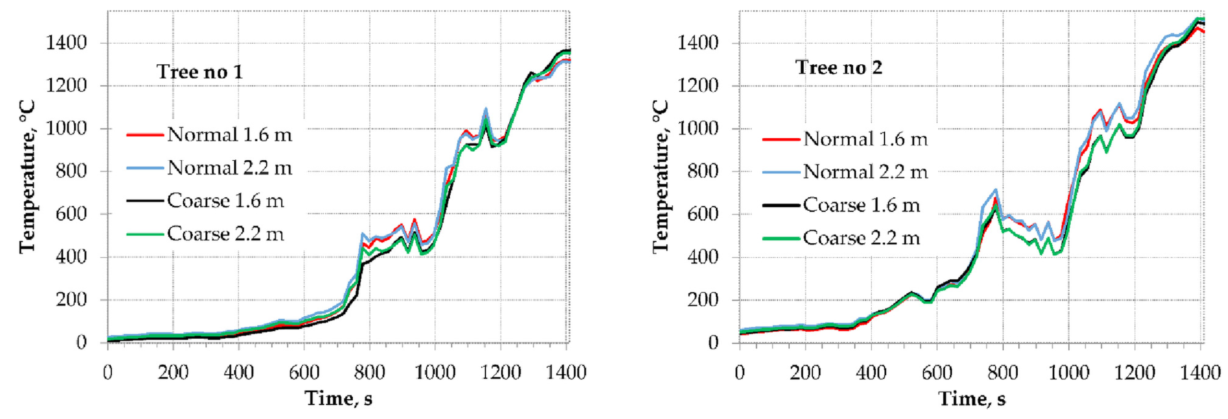
2.3.5. Mesh Sensitivity Analysis

Since the obtained results may depend on the applied numerical mesh, two different meshes were assessed. Both applied meshes were created according to the work presented by Węgrzyński et al. [48]. Since the fire plume impinges and starts to spread horizontally when in the above area, just beneath the ceiling, both meshes included inflation layers there. This helped to keep the accuracy of the flow image in this region. The burning pieces (the sofa and the table) were modeled using regular mesh, which contained only hexahedral cells. This allowed for a dense fragmentation with a relatively low number of mesh elements. The mixed mesh, containing mostly hexahedrons, was used for the whole room space, since such an approach allows for smooth transitions among elements of different sizes. The parameters of the applied meshes are shown in Table 3.
For comparison purposes, the temperature distributions close by and just above the sofa (trees 1 and 2) for both meshes are shown in Figure 10. The curves are quite similar despite some fluctuations, indicating that the model can be regarded as mesh independent.

2.4. FDS Model

The proposed approach was confronted with the well-recognized FDS software. Using this software, a model of the same furnished room was built. The model accurately reproduced the experimental setup. By default, FDS uses the large eddy simulation (LES) model for turbulence modeling. The combustion process is modeled similarly to the non-premixed model mentioned above [57]. It is an option in FDS to simulate material burnout by adopting a single-step pyrolysis (SSP) model in a way similar to that presented earlier. The other possibility is to use the ignition temperature-based pyrolysis (ITP) approach, in which the ignition temperature is set, then the value of the heat release rate per unit area (HRRPUA) is applied to calculate the burnout progress [58]. However, in both cases, there is a need to carefully adjust the control parameters by the trial and error method. The data published by Park and Kwark were very helpful here [59]. For the SSP approach, the parameters were tuned with an option of fitting the TGA curve (similarly as in the Fluent model). The parameters adopted for both material burnout approaches are listed in Table 4.
The computational domain of the model consisted of a number of meshes, which allowed for applying a dense mesh (cell edge of 0.05 m) to model the combustible items and their vicinity, and a coarse mesh (cell edge of 0.1 m) for the other parts of the compartment. These values were in accordance with the NIST recommendation.
The quality of flow modeling for buoyant plumes depends on a non-dimensional term D*/δx, where δx denotes the cell size and D* is the characteristic fire diameter. The latter value is given as follows (ρ, cp and T are, respectively, density, specific heat and temperature of ambient air) [57]:
D * = ( Q ˙ ρ c p T g ) 2 5
During the addressed simulation, the heat release rate ( Q ˙ ) varied, but assuming the maximum reasonable value of 1.2 MW [46], D* was estimated to be approximately 1 m. There are no explicit tips on how to establish the ratio D*/δx in advance, but in this work this value was 10 and 20 (depending on the mesh), which was consistent with the examples provided by NIST [57]. Hence, no additional mesh sensitivity analysis is discussed.

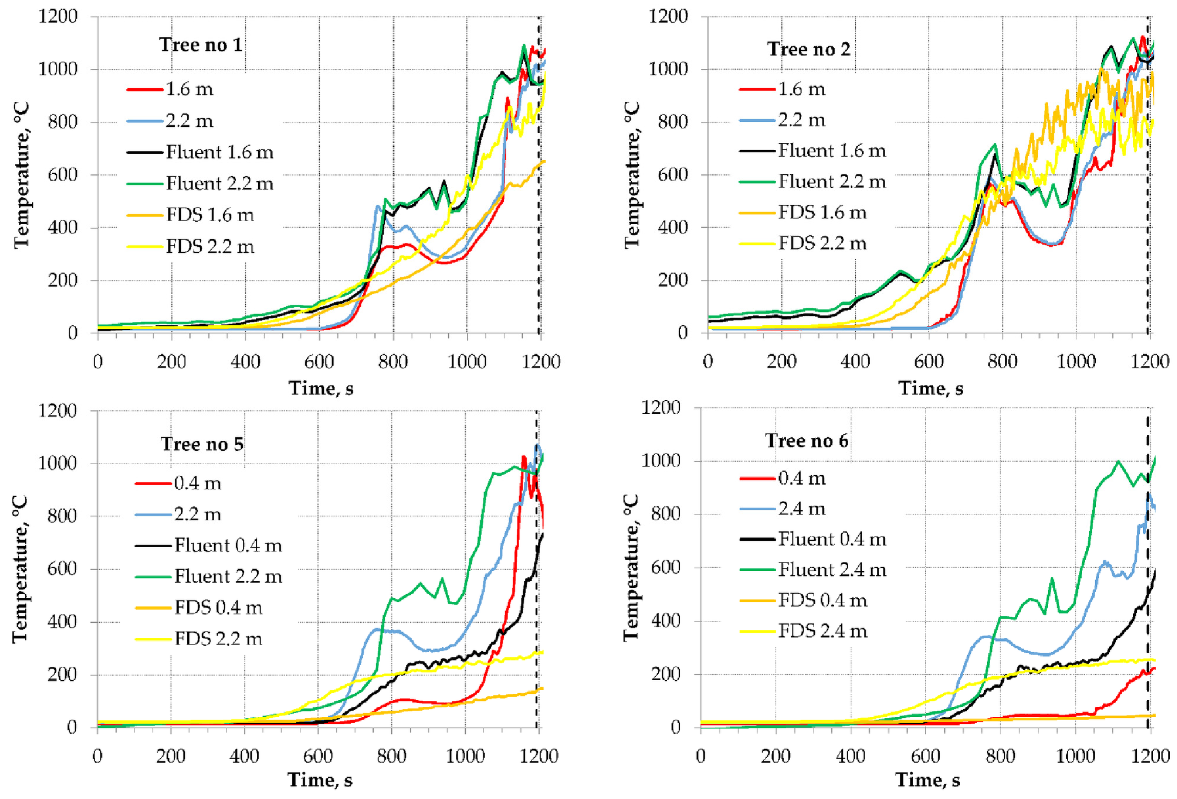
3. Results—Model Validation and Discussion

Since the first fire test was aborted before the fire could reach its maximum intensity, data from the second fire were used to validate the numerical model. The comparison of real and modeled temperature distributions is shown in Figure 11. In this experiment, the windows broke at 1193 s of fire development, and due to a rapid cold air inflow, the temperature dropped. The numerical simulation did not take this event into account. Hence, both curves diverge at this point from each other. In such a situation, only the growth phase of the fire development should be considered when validating the model.
At first glance, one can see that the temperature distributions differ in some degree. It concerns mainly FDS results: the predicted temperatures are generally lower, but the stratification is clearer. The first local temperature maximum is not visible here in contrast to the real data and the Fluent results. Since this is the merit of the work, further analysis is focused on Fluent outcomes. Although the experimental and calculated-via-Fluent curves do not overlap exactly, their courses are very similar, and the maximum temperature values are almost the same. The differences are visible for both the temperature values (up to about 100–200 °C) and the pace the fire was developing (a shift of the forepeak up to 100 s).
The ignition process was going in a slightly different way: in the numerical model, the whole volume of the ignition source was patched to a temperature of 500 °C instead of a slow development, as in the reality. This was to speed up the calculation, but it influenced somewhat the temperature distribution in the first moments. Therefore, in the very initial stage, when only the kindling was burning (before 600 s), the calculated temperature became higher above the sofa (especially for tree no. 2).
The best match can be observed for tree no. 2, which may confirm the accuracy of the material combustion model. The moments of forepeak and the maximum temperature occurrence were in good agreement, although the calculated temperature is overestimated (sometimes up to almost 200 °C).
When analyzing data for trees no. 3 and 4, one can see that the temperature stratification observed in the experimental data is not as clear in the numerical results—the calculated curves corresponding to different heights are close to each other. In addition, for those thermocouple trees, the divergency of the calculated temperature was the highest—the pace of the temperature growth was reproduced accurately, but its values were still higher than measured (the gap sometimes exceeded even 200 °C). The same applies to other thermocouple trees placed at greater distances from the fire source, which are not shown here. This may indicate that the flows throughout the room were not reproduced in a desired level of precision.
However, considering the simplicity of the model, it can be regarded as reliable. It is important to consider that real fires can be fickle phenomena. The experiments ran in somewhat unrepeatable ways despite controlled conditions, which were kept the same as much as possible. For this reason, the principle of ‘consistent crudeness’ should be taken into account in fire engineering [60]. It assumes that in light of input data uncertainty and the general unpredictability of a fire, one does not need to try to achieve a very high accordance of a theoretical or a numerical model with a particular set of experimental data.
There is a clear forepeak visible in the majority of the temperature vs. time curves. It appears in both the experimental and numerical results, especially for thermocouples placed just above the burning sofa. The possible explanation is as follows:
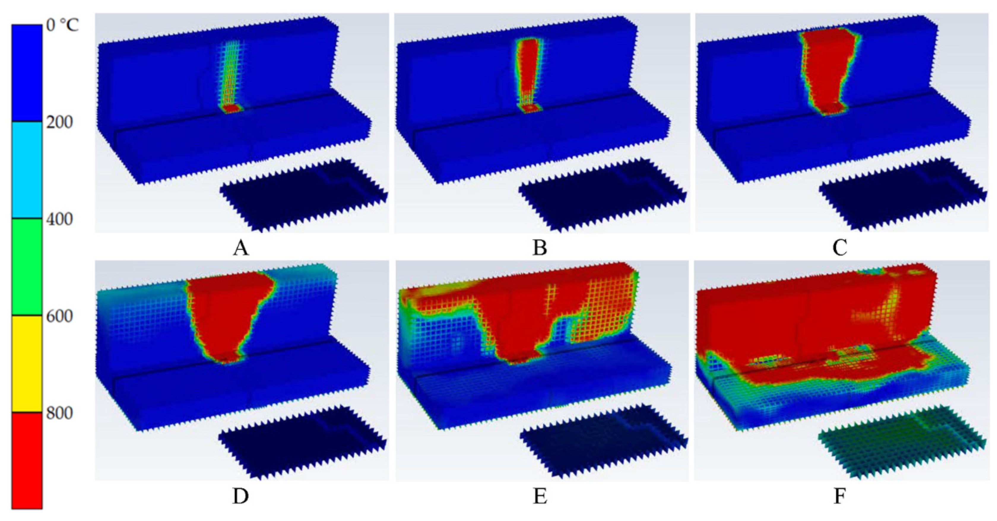
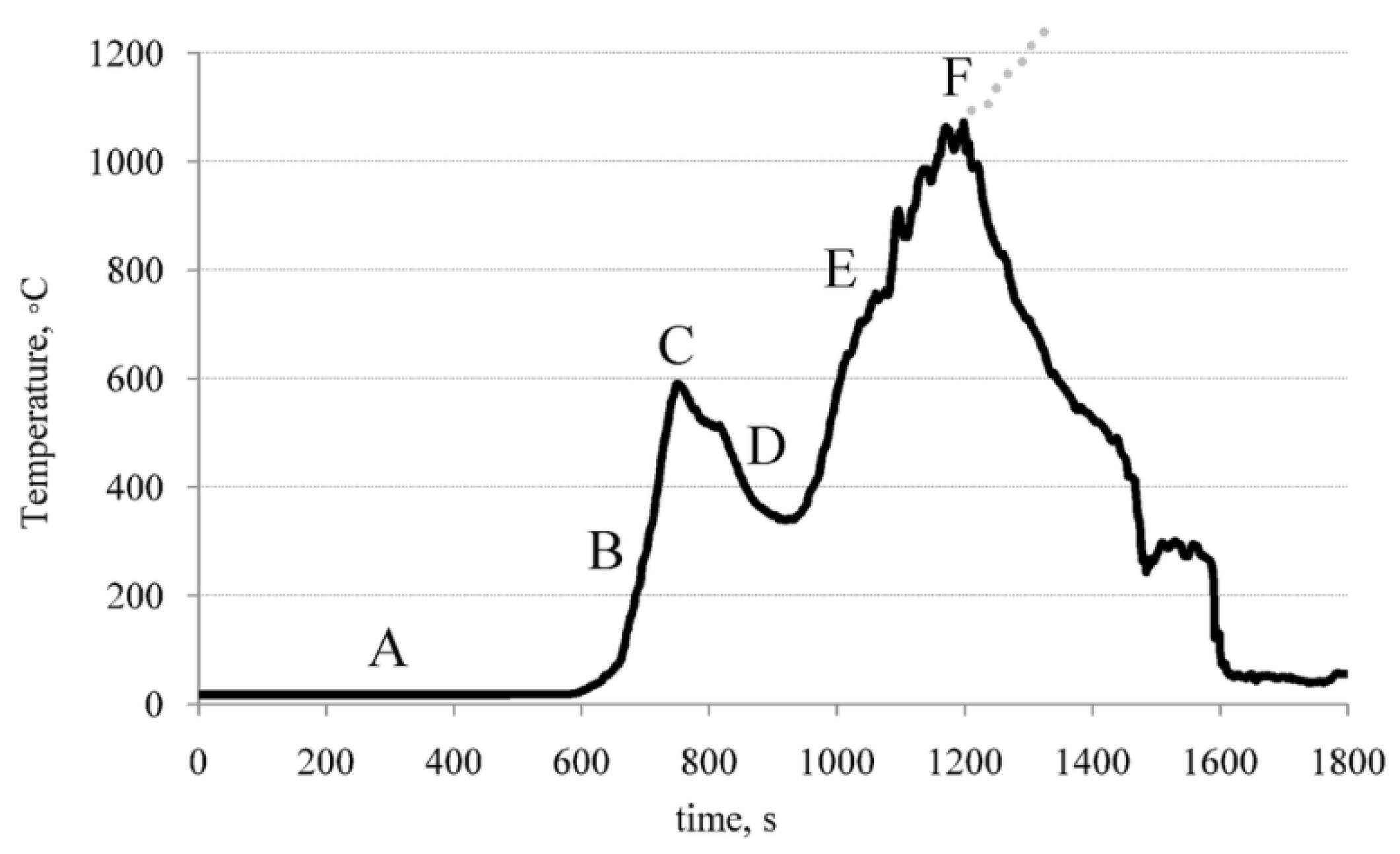
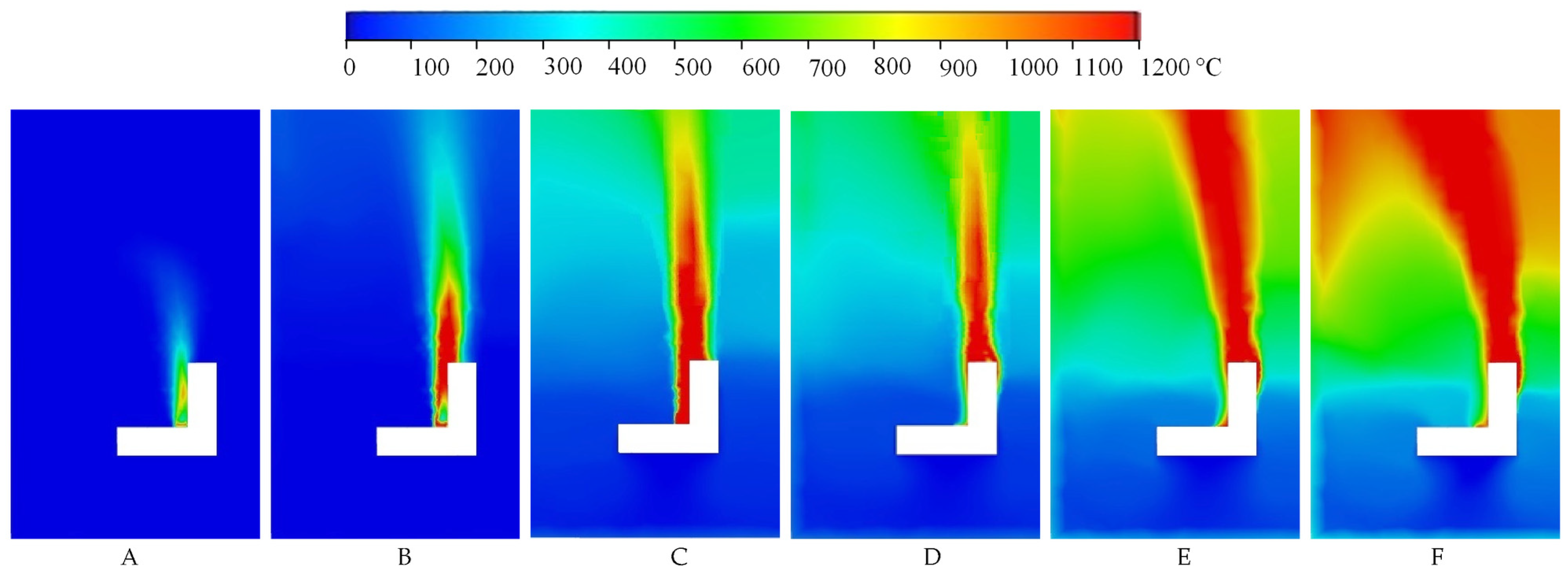
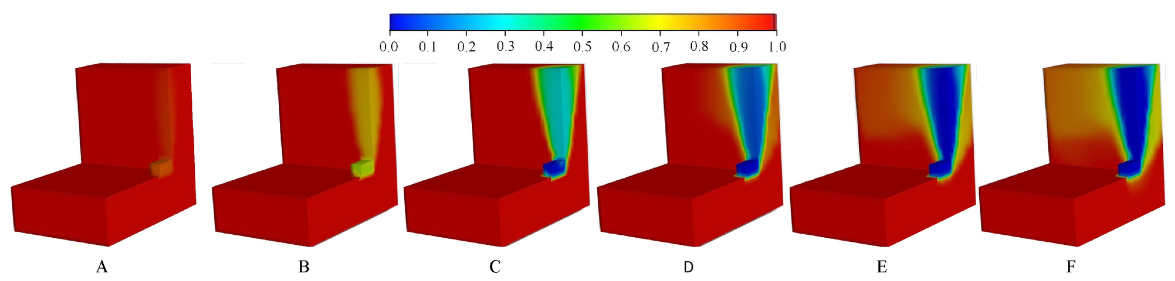
  • At the beginning of the process, the backrest foam needs more heat to ignite, and the only burning part is the kindling. Due to the low volume of the burning material, no significant temperature rise was observed.
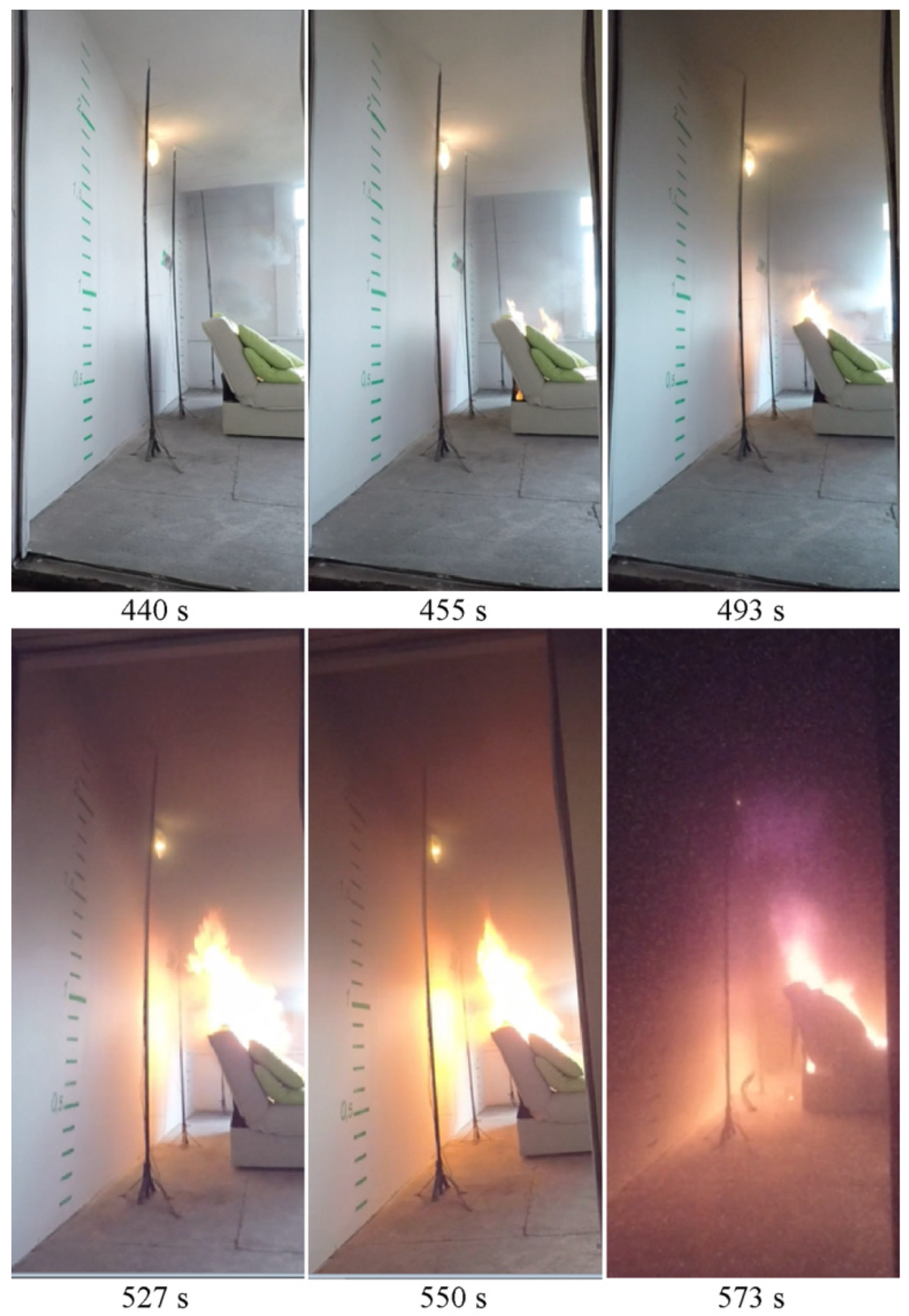
  • At the first stage of the fire development, the burning area slowly expands upwards and slightly on both sides, forming a u-shaped region of combustion that covers the subsequent parts of the sofa backrest, mainly due to the convectional transport of hot gases along the surface of the backrest and partially inside it because of its low porous resistance. This phase lasts to the moment where this region reaches the top of the backrest. At this phase, the volume of hot gases started to increase significantly, and a steep temperature rise was observed.
  • When the burning area reaches the top of the backrest, the fire development clearly slows down because its spread is hindered. This happens mainly horizontally by conductive heat transfer to adjacent parts of the backrest. This way of heat transfer is significantly less efficient due to the low thermal conductivity of the polyurethane foam.
  • Since the fire stops spreading quickly, the temperature above the fire source may even drop because the hot gases continue to spread along the ceiling. However, the combustion of the u-shaped area of the backrest continues and generates hot gases. Therefore, the layer of hot gases beneath the ceiling is gradually lowering.
  • When this layer reaches the top of the backrest, it causes the ignition of the upper part of the backrest, and the fire development is accelerated. A large part of the backrest is ignited, huge amounts of hot gases are generated and the hot layer lowers quickly, resulting in the fire quickly covering the sofa. The temperature rises significantly in this period.
  • In this phase, the layer of hot gases reaches far towards the room floor, and the fire may spread to other furniture items. The fire will develop to complete burnout if there is a sufficient fresh air supply or become under-ventilated in a smaller compartment.
These phases of the sofa fire development are shown in Figure 12, which presents the burning areas, and are marked in Figure 13, where a diagram of temperature distribution just above the sofa is shown (the grey dotted line marks the expected temperature rise if the windows had not fallen out). The last image in Figure 4 (timestamp 573 s) corresponds to a time moment between phases D and E; later, the large amounts of soot made the movie completely unreadable.
Figure 14 presents a snapshot taken at phase C during the first fire test. This corresponds to the frame at 493 s in Figure 4. It was almost the last moment a clear photo could be taken because, in a dozen seconds, wisps of smoke began to appear from the lowering smoke layer.
The temperature distributions in the compartment at the sofa symmetry plain at these moments are shown in Figure 15. The lowering layer of hot gases is clearly visible there (C–E); the same applies to the moment when this layer reached the sofa and the fire development started to accelerate €.
Figure 16 shows the burnout of the sofa material at the same time moments (the sofa is cut by a symmetry plane, the volume corresponding to the ignition source is also shown). The observations are in line with the earlier ones. At phases B, C and D, the conical burning region was developing, but due to the low heat conductance of polyurethane foam, its horizontal spread was slow. In phases C and D, the fire was kept alive mainly due to the burnout of the material in this region rather than its spreading.
The phase marked as C is critical for fire development. This applied to both real and numerical experiments. Some real fire experiments ceased to develop at this stage. This was presumably due to slight differences in experimental conditions. It might concern the properties of polyurethane foam, which resulted from different storage conditions, despite all used sofas being exactly of the same type.
As was mentioned earlier, there was no forepeak visible in the FDS results, so the FDS simulation did not reproduce the process of fire development in such a faithful manner. However, it generally revealed a similar way of spreading the fire. As an example, the burnout progress corresponding to phase E is shown in Figure 17.
A necessary condition for the numerical model to achieve conformity with the experimental data was to adjust the parameters controlling the intensity of pyrolysis and the density of flammable material. A threshold condition was revealed here: if the pyrolysis intensity was high enough, the fire spread quite quickly over the entire item in all directions. Otherwise, the u-shaped burning region at the backrest was formed and then it spread slowly. The burning area surrounding the ignition source barely spread horizontally. Meanwhile, the height of hot layer gases in the compartment was lowering continuously and if the fuel amount was large enough to sustain the fire, it reached the sofa and caused the violent fire revival and expansion.

4. Conclusions

First, this work presents full-scale fire experiments on fire development in a furnished room in a high-rise building. Such experiments are rare due to high costs and the many organizational obstacles. Then, the second stage of the work involved numerical simulations, allowing investigators to deepen their knowledge of the processes involved during fire development in furnished spaces and explore more than the actual experimental configurations. Two software packages were used, FDS and ANSYS Fluent. The results of both numerical models were generally consistent with the real process of fire spreading. However, those of Fluent reproduced the fire development phases in a more accurate way. In particular, since the Fluent model had to be built from scratch it allowed for accurate examining of the process of fire spreading.
Despite its relative simplicity, the proposed numerical model was able to mimic the development of the real fire. This gives hope for reaping the benefits of ANSYS Fluent capabilities in more sophisticated configurations of numerical models. However, as some clear divergences between measured and calculated temperature fields were observed, the basic model of fire spread over a single furniture item should be improved in the future. The maximum calculated temperature appeared to be overestimated, and the temperature increase rate was also higher than the real one. However, eventually, the simulated fires did not differ from the real ones to a higher degree than the real fires differed from each other. This means that there are some unknown and variable factors that can influence the course of fire development. Even though the real experiment was prepared with care to details, and thus so was the numerical model, these factors evidently were beyond researchers’ control and knowledge. Anyway, despite their influence being noted, it did not alter the observed phenomena to a significant degree.
The numerical research revealed a threshold condition for fire spreading over an upholstered item. If a combustible material is less susceptible to pyrolysis, the fire spreads rather slowly and only lowering the layer of hot gases may cause the violent fire development.
Both real and numerical experiments showed non-uniform temperature distribution in the test room. This was especially visible in the fire growth phase when clear temperature stratification was observed. However, while the stratification almost ceased, the experiments did not enter the stage where the spatial temperature distribution would be more even. This could be regarded as an indicator to apply more measurement points in the future to record the results of such experiments more accurately.

Author Contributions

Conceptualization, M.K. and A.K.; methodology, M.K.; software, A.K.; validation, M.K. and A.K.; data curation, M.K. and A.K.; writing—original draft preparation, M.K. and A.K.; visualization, A.K. and M.K. All authors have read and agreed to the published version of the manuscript.

Funding

The publication of the work was supported by the Polish Ministry of Science and Higher Education, within statutory research subsidy 08/010/BK22/0060.

Data Availability Statement

Not applicable.

Acknowledgments

The authors would like to thank the Smay Company for the opportunity for participation in the research, for the provided management support and for the consent to publish the results. We would like also to thank the Headquarters of the State Fire Service in Sosnowiec for supervision, security and participation in the research.

Conflicts of Interest

The authors declare no conflict of interest.

References

  1. Lange, D.; Torero, J.L.; Osorio, A.; Lobel, N.; Maluk, C.; Hidalgo, J.P.; Johnson, P.; Foley, M.; Brinson, A. Identifying the attributes of a profession in the practice and regulation of fire safety engineering. Fire Saf. J. 2021, 121, 103274. [Google Scholar] [CrossRef]
  2. Chu, G.; Sun, J. Decision analysis on fire safety design based on evaluating building fire risk to life. Saf. Sci. 2008, 46, 1125–1136. [Google Scholar] [CrossRef]
  3. Chu, G.Q.; Chen, T.; Sun, Z.H.; Sun, J.H. Probabilistic risk assessment for evacuees in building fires. Build. Environ. 2007, 42, 1283–1290. [Google Scholar] [CrossRef]
  4. Zhao, C.M.; Lo, S.M.; Lu, J.A.; Fang, Z. A simulation approach for ranking of fire safety attributes of existing buildings. Fire Saf. J. 2004, 39, 557–579. [Google Scholar] [CrossRef]
  5. Chen, Z.; Satoh, K.; Wen, J.; Huo, R.; Hu, L. Burning behavior of two adjacent pool fires behind a building in a cross-wind. Fire Saf. J. 2009, 44, 989–996. [Google Scholar] [CrossRef]
  6. Khan, A.; Usmani, A.; Torero, J.L. Evolution of fire models for estimating structural fire-resistance. Fire Saf. J. 2021, 124, 103367. [Google Scholar] [CrossRef]
  7. Wang, L.; Li, W.; Weimin, W.; Yang, R. Fire risk assessment for building operation and maintenance based on BIM technology. Build. Environ. 2021, 205, 108188. [Google Scholar] [CrossRef]
  8. Harmathy, T.Z. A New Look at Compartment Fires. Fire Technol. 1972, 8, 196–217. [Google Scholar] [CrossRef]
  9. Thomas, P.H.; Heselden, A.J.; Law, M. Fully-Developed Compartment Fires—Two Kinds of Behavior; H.M. Stationery Office: Richmond, UK, 1967. [Google Scholar]
  10. Torero, J.L.; Majdalani, A.H.; Abecassis-Empis, C.; Cowlard, A. Revisiting the compartment fire. Fire Saf. J. 2014, 11, 28–45. [Google Scholar] [CrossRef]
  11. Hua, J.; Wang, J.; Kumar, K. Development of a hybrid field and zone model for fire smoke propagation simulation in buildings. Fire Saf. J. 2005, 40, 99–119. [Google Scholar] [CrossRef]
  12. Zhang, J.Y.; Lu, W.Z.; Huo, R.; Feng, R. A new model for determining neutral-plane position in shaft space of a building under fire situation. Build. Environ. 2008, 43, 1101–1108. [Google Scholar] [CrossRef]
  13. Prasad, K.; Baum, H.R. Coupled fire dynamics and thermal response of complex building structures. Proc. Combust. Inst. 2005, 30, 2255–2262. [Google Scholar] [CrossRef]
  14. Stern-Gottfried, J.; Rein, G.; Bisby, L.; Torero, J.L. Experimental review of the homogeneous temperature assumption in post-flashover compartment fires. Fire Saf. J. 2010, 45, 249–261. [Google Scholar] [CrossRef] [Green Version]
  15. Jahn, W.; Rein, G.; Torero, J.L. A posteriori modelling of the growth phase of Dalmarnock Fire Test One. Build. Environ. 2011, 46, 1065–1073. [Google Scholar] [CrossRef]
  16. Gupta, V.; Hidalgo, J.; Cowlard, A.; Abecassis-Empis, C.; Majdalani, H.A.; Maluk, C.; Torero, J.L. Ventilation effects on the thermal characteristics of fire spread modes in open-plan compartment fires. Fire Saf. J. 2021, 120, 103072. [Google Scholar] [CrossRef]
  17. Sun, X.; Hu, L.; Zhang, X.; Yang, Y.; Ren, F.; Fang, X.; Wang, K.; Lu, H. Temperature evolution and external flame height through the opening of fire compartment: Scale effect on heat/mass transfer and revisited models. Int. J. Therm. Sci. 2021, 164, 106849. [Google Scholar] [CrossRef]
  18. Lu, K.; Wang, Z.; Ding, Y.; Wang, J.; Zhang, J.; Delichatsios, M.; Hu, L. Flame behavior from an opening at different elevations on the facade wall of a fire compartment. Proc. Combust. Inst. 2021, 38, 4551–4559. [Google Scholar] [CrossRef]
  19. Bonner, M.; Węgrzyński, W.; Papis, B.; Rein, G. KRESNIK: A top-down, statistical approach to understand the fire performance of building face des Rusing standard test data. Build. Environ. 2020, 169, 106540. [Google Scholar] [CrossRef]
  20. Mckenna, S.; Jones, N.; Peck, G.; Dickens, K.; Pawelec, W.; Oradei, S.; Harris, S.; Stec, A.; Hull, R. Fire behavior of modern façade materials–Understanding the Grenfell Tower fire. J. Hazard. Mater. 2019, 368, 115–123. [Google Scholar] [CrossRef]
  21. Sharma, A.; Mishra, K.B. Experimental investigations on the influence of ‘chimney-effect’ on fire response of rain screen façades in high-rise buildings. J. Build. Eng. 2021, 44, 103257. [Google Scholar] [CrossRef]
  22. Chow, C.L.; Chow, W.K. Heat release rate of accidental fire in a supertall building residential flat. Build. Environ. 2010, 45, 1632–1640. [Google Scholar] [CrossRef]
  23. Cheng, C.C.K. fire safety study of Hong Kong refuge floor building wall layout design. Fire Saf. J. 2009, 44, 545–558. [Google Scholar] [CrossRef]
  24. Ren, F.; Hu, L.; Zhang, X.; Sun, X.; Fang, X. Temperature evolution from stratified- to well-mixed condition inside a fire compartment with an opening subjected to external wind. Proc. Combust. Inst. 2021, 38, 4495–4503. [Google Scholar] [CrossRef]
  25. Lu, K.; Xu, H.; Shi, C.; Wang, Z.; Wang, J.; Ding, Y. Numerical investigation of air curtain jet effect on the upper layer temperature evolution of a compartment fire and its transition. Appl. Therm. Eng. 2021, 197, 117409. [Google Scholar] [CrossRef]
  26. Chen, C.-J.; Hsieh, W.-D.; Hu, W.-C.; Lai, C.-M.; Lin, T.-H. Experimental investigation and numerical simulation of a furnished office fire. Build. Environ. 2010, 45, 2735–2742. [Google Scholar] [CrossRef]
  27. Majdalani, A.H.; Cadena, J.E.; Cowlard, A.; Munoz, F.; Torero, J.L. Experimental characterization of two fully-developed enclosure fire regimes. Fire Saf. J. 2016, 79, 10–19. [Google Scholar] [CrossRef]
  28. Yang, P.; Tan, X.; Xin, W. Experimental study and numerical simulation for a storehouse fire accident. Build. Environ. 2011, 46, 1445–1459. [Google Scholar] [CrossRef]
  29. Byström, A.; Cheng, X.; Wickström, U.; Veljkovic, M. Full-scale experimental and numerical studies on compartment fire under low ambient temperature. Build. Environ. 2012, 51, 255–262. [Google Scholar] [CrossRef]
  30. Mackay, D.; Barber, T.; Yeoh, G.H. Experimental and computational studies of compartment fire behavior training scenarios. Build. Environ. 2010, 45, 2620–2628. [Google Scholar] [CrossRef]
  31. Hasib, R.; Kumar, R.; Kumar, S.; Kumar, S. Simulation of an experimental compartment fire by CFD. Build. Environ. 2007, 42, 3149–3160. [Google Scholar] [CrossRef]
  32. He, Q.; Liu, N.; Xie, X.; Zhang, L.; Zhang, L.; Zhang, Y.; Yan, W. Experimental study on fire spread over discrete fuel bed—Part I: Effects of packing ratio. Fire Saf. J. 2021, 126, 103470. [Google Scholar] [CrossRef]
  33. He, Q.; Liu, N.; Xie, X.; Zhang, L.; Lei, J.; Zhang, Y.; Wu, D. Experimental study on fire spread over discrete fuel bed—Part II: Combined effects of wind and packing ratio. Fire Saf. J. 2022, 128, 103520. [Google Scholar] [CrossRef]
  34. Gupta, V.; Torero, J.L.; Hidalgo, J. Burning dynamics and in-depth flame spread of wood cribs in large compartment fires. Combust. Flame 2021, 228, 42–56. [Google Scholar] [CrossRef]
  35. ANSYS Fluent Theory Guide; Release 15.0; ANSYS, Inc.: Canonsburg, PA, USA, 2013.
  36. National Instruments. NI-9213 Specifications, 16-CH, ±78 mV, 24 Bit, 75 S/s Aggregate. Available online: https://www.ni.com/docs/en-US/bundle/ni-9213-specs/page/specifications.html (accessed on 21 November 2022).
  37. BS 5852-2006; Methods of Test for Assessment of the Ignitability of Upholstered Seating by Smouldering and Flaming Ignition Sources. BSI: London, UK, 2006.
  38. Tlili, O.; Mhiri, H.; Bournot, P. Empirical correlation derived by CFD simulation on heat source location and ventilation flow rate in a fire room. Energy Build. 2016, 122, 80–88. [Google Scholar] [CrossRef]
  39. Król, A.; Król, M.; Krawiec, S. A Numerical Study on Fire Development in a Confined Space Leading to Backdraft Phenomenon. Energies 2020, 13, 1854. [Google Scholar] [CrossRef]
  40. Modest, M.F. Radiative Heat Transfer, 3rd ed.; Elsevier Inc.: Amsterdam, The Netherlands, 2013; pp. 279–302. [Google Scholar]
  41. Safarzadeh, M.; Heidarinejad, G.; Pasdarshahri, H. The effect of vertical and horizontal air curtain on smoke and heat control in the multi-storey building. J. Build. Eng. 2021, 40, 102347. [Google Scholar] [CrossRef]
  42. Sivathanu, Y.R.; Faeth, G.M. Generalized State Relationships for Scalar Properties in Non-Premixed Hydrocarbon/Air Flames. Combust. Flame 1990, 82, 211–230. [Google Scholar] [CrossRef] [Green Version]
  43. Jones, W.P.; Whitelaw, J.H. Calculation Methods for Reacting Turbulent Flows, A Review. Combust. Flame 1982, 48, 1–26. [Google Scholar] [CrossRef]
  44. Pope, S.B. Pdf methods for turbulent reactive flows. Prog. Energy Combust. Sci. 1985, 11, 119–192. [Google Scholar] [CrossRef]
  45. Glicksman, L.; Schuetx, M.; Sinofsky, M. Radiation heat transfer in foam insulation. Int. J. Heat Mass Transf. 1987, 30, 187–197. [Google Scholar] [CrossRef]
  46. Eschenbacher, A.; Varghese, R.J.; Weng, J.; van Geem, K.M. Fast pyrolysis of polyurethanes and polyisocyanurate with and without flame retardant: Compounds of interest for chemical recycling. J. Anal. Appl. Pyrolysis 2021, 160, 105374. [Google Scholar] [CrossRef]
  47. Font, R.; Fullana, A.; Caballero, J.A.; Candela, J.; Garcia, A. Pyrolysis study of polyurethane. J. Anal. Appl. Pyrolysis 2001, 58–59, 63–77. [Google Scholar] [CrossRef]
  48. Węgrzyński, W.; Lipecki, T.; Krajewski, G. Wind and Fire Coupled Modelling–Part II: Good Practice Guidelines. Fire Technol. 2018, 54, 1443–1485. [Google Scholar] [CrossRef]
  49. Hopkin, C.; Spearpoint, M.; Bittern, A. Using experimental sprinkler actuation times to assess the performance of Fire Dynamics Simulator. Fire Saf. J. 2018, 36, 342–361. [Google Scholar] [CrossRef]
  50. Węgrzyński, W.; Vigne, G. Experimental and numerical evaluation of the influence of the soot yield on the visibility in smoke in CFD analysis. Fire Saf. J. 2017, 91, 389–398. [Google Scholar] [CrossRef]
  51. Jomaa, G.; Goblet, P.; Coquelet, C.; Morlot, V. Kinetic modeling of polyurethane pyrolysis using non-isothermal thermogravimetric analysis. Thermochim. Acta 2015, 612, 10–18. [Google Scholar] [CrossRef] [Green Version]
  52. Cheng, Y.; Xu, Z.; Chen, S.; Ji, Y.; Zhang, D.; Liang, J. The influence of closed pore ratio on sound absorption of plant-based polyurethane foam using control unit model. Appl. Acoust. 2021, 180, 108083. [Google Scholar] [CrossRef]
  53. Garrido, M.A.; Font, R. Pyrolysis and combustion study of flexible polyurethane foam. J. Anal. Appl. Pyrolysis 2015, 113, 202–215. [Google Scholar] [CrossRef] [Green Version]
  54. McGrattan, K.; Hostikka, S.; Mcdermott, R.; Floyd, J.; Weinschenk, C.; Overholt, K. FDS Validation Guide; NIST Publications: Gaithersburg, MD, USA, 2013. [Google Scholar]
  55. LA Nasa, J.; Biale, G.; Ferriani, B.; Colombini, M.P.; Modugno, F. A pyrolysis approach for characterizing and assessing degradation of polyurethane foam in cultural heritage objects. J. Anal. Appl. Pyrolysis 2018, 134, 562–572. [Google Scholar] [CrossRef]
  56. Król, A.; Jahn, W.; Krajewski, G.; Król, M.; Węgrzyński, W. A Study on the Reliability of Modeling of Thermocouple Response and Sprinkler Activation during Compartment Fires. Buildings 2022, 12, 12010077. [Google Scholar] [CrossRef]
  57. McGrattan, K.; Hostikka, S.; Floyd, J.; McDermontt, R.; Vanella, M. Fire Dynamics Simulator, Technical Reference Guide, Vol. 3: Validation; NIST Publication 1019: Gaithersburg, MD, USA, 2020. [Google Scholar] [CrossRef]
  58. Janardhan, R.K.; Hostikka, S. Predictive Computational Fluid Dynamics Simulation of Fire Spread on Wood Cribs. Fire Technol. 2019, 55, 2245–2268. [Google Scholar] [CrossRef] [Green Version]
  59. Park, J.; Kwark, J. Experimental Study on Fire Sources for Full-Scale Fire Testing of Simple Sprinkler Systems Installed in Multiplexes. Fire 2021, 4, 4010008. [Google Scholar] [CrossRef]
  60. Platt, D.; Elms, D.; Buchanan, A. A probabilistic model of fire spread with time effects. Fire Saf. J. 1994, 22, 367–398. [Google Scholar] [CrossRef]
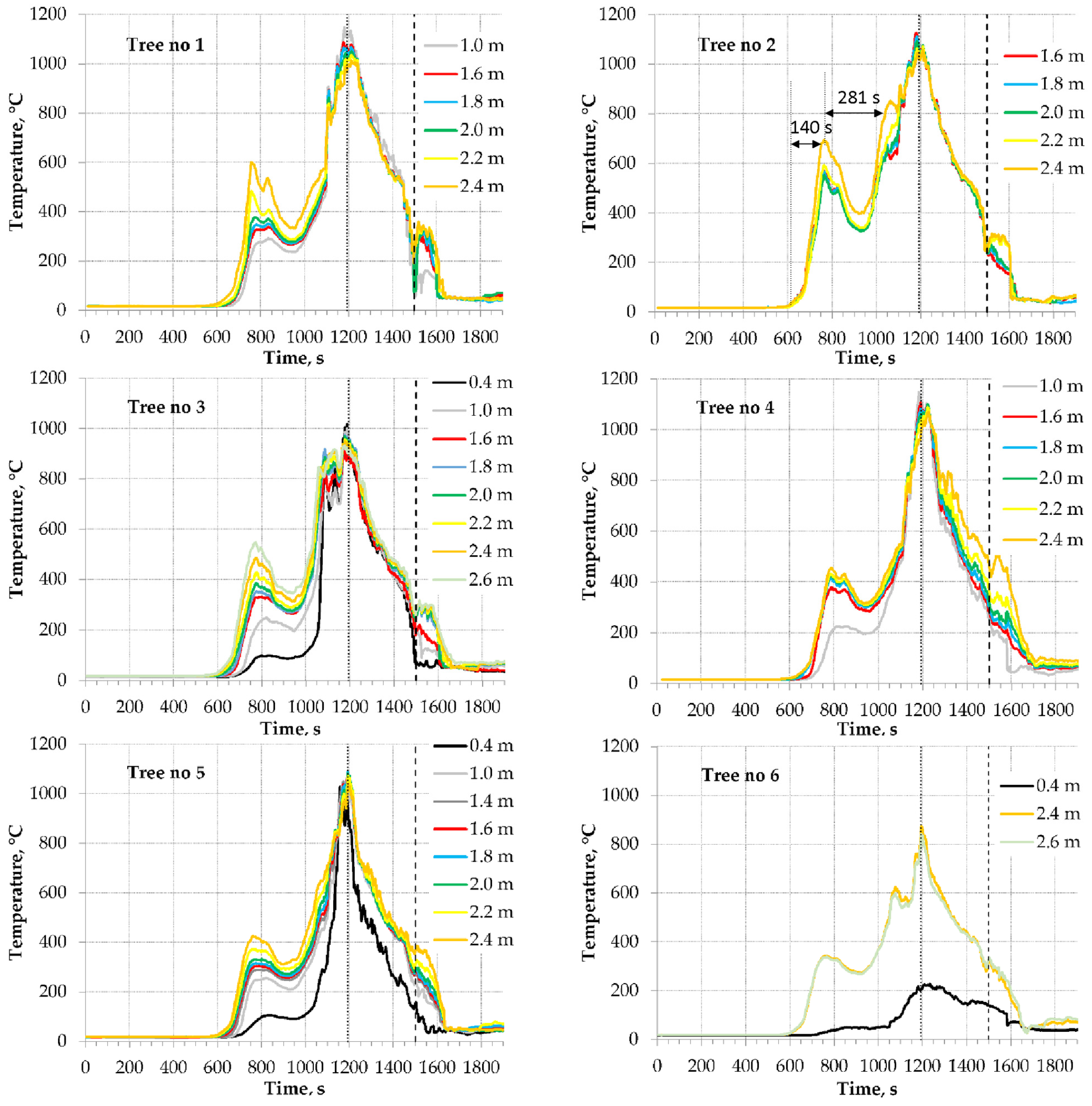
Figure 1. View of the building with the test room marked (on the west façade).
Buildings 12 02189 g001
Figure 2. The test room (distances given in mm).
Buildings 12 02189 g002
Figure 3. The location of the ignition source on the sofa at the beginning of a fire.
Buildings 12 02189 g003
Figure 4. Subsequent stages of fire development (the first test). Time in seconds from the moment of ignition.
Buildings 12 02189 g004
Figure 5. Temperatures during the first test. Dashed lines mark the beginning of the firefighting operations (790 s).
Buildings 12 02189 g005
Figure 6. Temperatures during the second test. Dashed lines mark the beginning of the firefighting operations (1500 s), dotted lines mark the moment windows fell out (1193 s).
Buildings 12 02189 g006
Figure 7. Windows breaking during the second test fire.
Buildings 12 02189 g007
Figure 8. A Fluent model of the partially furnished compartment.
Buildings 12 02189 g008
Figure 9. Comparison of modeled pyrolysis rate with experimental data [53,54,55].
Buildings 12 02189 g009
Figure 10. Numerical results for two mesh densities.
Buildings 12 02189 g010
Figure 11. Comparison of the selected temperature distributions for real and modeled (Fluent and FDS—ITP approach) fire.
Buildings 12 02189 g011
Figure 12. The subsequent phases of sofa fire development: temperature distribution on its surface (description in text).
Buildings 12 02189 g012
Figure 13. The phases of sofa fire marked at the temperature curve (the second fire test, tree no. 2, height 2.4 m in Figure 6) (description in text).
Buildings 12 02189 g013
Figure 14. An image of u-shaped burning region (about 493 s of the first fire test).
Buildings 12 02189 g014
Figure 15. Temperature distributions at the sofa symmetry plain at selected moments (description in text).
Buildings 12 02189 g015
Figure 16. Progress of the material burnout (0 corresponds to the complete burnout) (description in text).
Buildings 12 02189 g016
Figure 17. Material burnout in FDS simulation corresponding to phase E.
Buildings 12 02189 g017
Table 1. Summary of thermocouple trees.
Number of the TreeThe Heights of the Thermocouples on the Trees [mm]
(Measured from the Floor)
11000, 1600, 1800, 2000, 2200, 2400
21600, 1800, 2000, 2200, 2400
3400, 1000, 1400, 1800, 2000, 2200, 2400, 2600
41000, 1600, 1800, 2000, 2200, 2400
5400, 1400, 1600, 1800, 2000, 2200, 2400
6400, 2400, 2600
Table 2. The meteorological conditions during both fire tests.
Fire Test 1Fire Test 2
Air temperature 2 m above the ground, °C1810
Air temperature 100 m above the ground (approx. 5 m above the roof of the building), °C168
Wind speed 10 m above ground (10 min average), m/s2.33.8
Wind speed 100 m above ground (10 min average), m/s3.77.0
Wind directionwestwest
Table 3. Parameters of the applied meshes.
MeshNo. of ElementsNo. of NodesNo. of Inflation LayersEdge Length
RoomBurning Items
Normal470,362118,188100.1500.050
Coarse319,89881,41880.2000.075
Table 4. Parameters of material burnout.
ParameterValue
Heat of combustion, kJ/kg2.54 × 104
Heat of reaction, kJ/kg1.57 × 103
SSPReference temperature, °C100.0
Heating rate, K/min5.0
Pyrolysis range, °C80.0
Mass Fraction Exponent (ns)2.0
ITPHRRPUA, kW/m2600.0
Ignition temperature, °C300.0
Time ramp
(relative intensity vs. time)
0 s0.0
60 s1.0
120 s0.8
240 s0.2
Publisher’s Note: MDPI stays neutral with regard to jurisdictional claims in published maps and institutional affiliations.

