Design of Structural Steel Components According to Manufacturing Possibilities of the Robot-Guided DED-Arc Process

Abstract

Additive manufacturing with the DED-arc process offers limited freedom in terms of the geometric shape of work pieces. The process and fabrication systems restrict the part geometry producible, which must be taken into account during design already. For this reason, a design process was investigated in which geometry generation is based on a self-organizing system. The aim of using a self-organizing system is the possibility to directly control the geometry-defining points. Next to load cases, the design method considers geometric boundary conditions from the production process when generating the geometry. In order to identify these geometrical constraints from production experimentally, a concept of Case Study Demonstrators was applied. This was used to investigate how path planning and production can be carried out for specific geometrical features and to identify restraints of the process and the manufacturing system, e.g., smallest producible wall thickness and overhangs. Subsequently, the obtained restraints were considered as boundary conditions for the design process and were included in the modification of an example geometry. By applying the presented design method, it was possible to maintain a minimum wall thickness throughout the structure while generating a topologically optimized geometry. In contrast to compliance with the minimum wall thickness, no satisfactory behavioral rule could be found for limiting the overhang.

1. Introduction

Since 1991, the relative total productivity of industry workers has increased significantly. Figure 1 shows the development of relative work productivity of German industry workers since the German reunion in 1990 [1]. Opposite to the processing and manufacturing industry, this positive trend could not be observed in the construction industry. Major reasons for the significant increase in the manufacturing and processing sectors are increased automation and digitalization, while the construction industry is still dominated by manual work. Accordingly, automated production processes could help to achieve more economical construction processes also in construction industry.

Additive manufacturing (AM) is a disruptive manufacturing technology, which may help to overcome such hurdles within the next decades. It is a digitalized and automated production method, which generates components by subsequent deposition of material, mostly through layer-by-layer material deposition.

The structural and architectural design of construction elements has always been influenced by the applicable production processes. Accordingly, the design according to manufacturing possibilities needs to be redefined for AM principles. This article addresses the interdependency of design and manufacturing of AM components made from steel. The research presented was conducted within the collaborative research centre TRR 277 “Additive Manufacturing in Construction AMC” in close cooperation of structural designers and welding engineers.

1.1. DED-Arc of Metallic Components in AMC

With regard to structural steel components, the use of semi-finished parts and their processing are, nowadays, state of the art. The geometric complexity of steel structures constantly increases the demand for individual solutions, for instance, for the connection of two and more structural members. Such connection nodes are currently produced either by casting or with high manual effort by fusion welding of individual parts, which are manufactured from semi-finished products by subtractive processes. Buchanan and Gardner have reviewed the potential of AM for metal components in the construction industry [1]. They highlighted benefits such as reduction of material and waste, manufacturing of load-path optimized structures, and functionally graded materials. On the other hand, they also pronounced challenges for the education of engineers and workers, architectural and structural design, and quality inspection. In terms of AM methods for the manufacturing of large metal components, the benefit of wire-based AM-processes was discussed by Ding et al. [2]. They reviewed possible energy sources and manufacturing approaches with regard to process classification, achievable geometric accuracy, resolution, and deposition rate. Furthermore, they discussed process related parameters such as welding directions, residual stress, and resulting material parameters. With respect to DED-arc (DED: direct energy deposition), they identified the challenge of distortion and surface properties. DebRoy et al. provided an extended review on AM of metal components comparing available processes and materials, with a focus on resulting material and component properties, with similar findings [3].

The robot-guided DED-arc method establishes a layer-wise material deposition by melting wire electrodes in the electric arc at a high energy input [4]. The relative movement between welding torch and AM component is realized by robots or CNC-controlled kinematics. The DED-arc process is capable of combining high process efficiency with a high degree of geometric freedom. Additionally, the superior deposition rate allows for the fabrication of large-scale steel components achieving defined mechanical material properties. Furthermore, the potential for automation of this process is high. Feucht et al. investigated the potential use of this technology for local reinforcements and the generation of connection elements [5]. Reimann et al. studied the topology optimized design of steel connectors produced by DED-arc and highlighted the process chain of production, beginning from design to component manufacturing [6]. Despite the emerging possibilities, they also highlighted the need for post-processing of DED-arc components, due to variations of scale and form. Next to the challenges of manufacturing, the resulting material properties need to be addressed in the design process as well. This causes demand for advanced material and component testing. Rafieazad et al. tested DED-arc components made from low-carbon low-alloy steel wire (G3 Si 1, EN ISO 14341-A) [7]. They proved similar tensile properties in welding and building direction except for the elongation at fracture, which was significantly lower in building direction. This difference was associated with coarse grained microstructure at reheated inter-layer boundaries. Bourlet at al. investigated high strength filler metal G69 6 M21 Mn4Ni1.5CrMo (EN ISO 16834-A) for use in the DED-Arc process and determined the resulting microstructure, charpy impact toughness, and tensile parameters [8]. They proved retained austenite and applied heat treatment for its removal. They compared the resulting material parameters of as-deposited and heat treated material. The yield strength increased with the application of the heat treatment. Rodrigues et al. built DED-Arc specimens from high strength alloy G79 5 M21 Mn4Ni1.5CrMo (EN ISO 16834-A) under different variations of manufacturing parameters [9]. They found inhomogeneous cooling rates with increasing build-up height. The elongation at fracture was lower in the welding direction compared to the building direction. The ultimate tensile strength ranged between 700 MPa and 800 MPa, and did not reach the nominal strength of the filler metal when applied properly in fusion welding applications. However, the applied process strategy of constant waiting time between layers led to comparably high interpass temperatures of 300 °C to 550 °C, which may have altered the material properties significantly. Therefore, working with a constant interpass temperature is recommended with regard to the homogeneity of material properties.

However, since for AM technologies the design of the part must be linked to the possibilities of the manufacturing system, the applied manufacturing process, and the parameters, there is a demand for new approaches for the consideration of manufacturing restrictions in the design process. This means that a design method is needed, which is able to take given manufacturing possibilities into account.

1.2. Design Methods for DED-Arc

In steel construction, geometric design has so far been highly formalized. This is possible because manufacturing usually involves the machining and joining of semi-finished products. With formalization, it was possible to create typified connections for the most common combinations of load case and beam geometry. In additive manufacturing such as DED-arc, this possibility no longer exists. The geometric freedom of manufacturing leads to a very high degree of individualization of each component. The goal is often to use the material as efficiently as possible. For this reason, a basic geometry is created in most cases, which is further subjected to topological optimization according to the load cases. This geometry is not directly suitable for production. Often there are still areas with load peaks within the geometry. The meshing of the geometry for topology optimization can also usually be seen in the exported geometry. For this reason, a further step needs to be carried out after the topology optimization in order to optimize the shape. This can be performed manually or automatically by using software.

As a next step, path planning must be carried out for this geometry, taking into account the manufacturing possibilities of the production system. Often, the geometry does not meet the necessary requirements to be considered directly ready for production. In this case, the geometry has to be manually changed. Some software solutions for path planning are already available, with the ability to adapt the geometry through the constraints of the fabrications process. With the creation of a printable path, the generation of the geometry is usually completed.

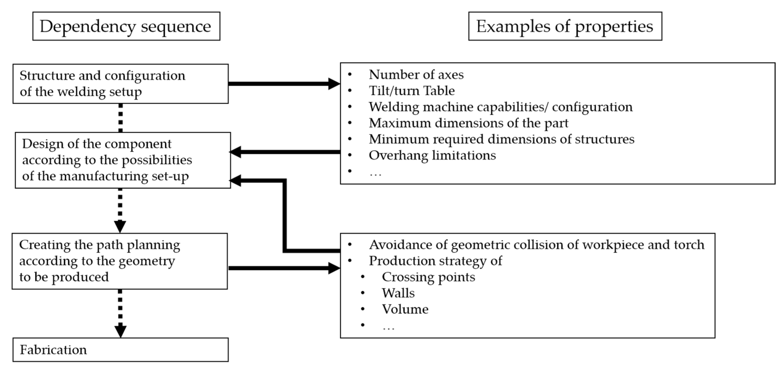
1.3. Manufacturing Strategies and Possibilities

For the manufacturing of complex parts, the geometry needs to be broken down to simple geometries representing the features that occur in the complex structure. By the manufacturing planning for those simple geometries, restrictions regarding geometrical features can be identified and taken into account during the design of the parts to be manufactured.

Before the realization of geometrical features such as overhangs, undercuts etc., the optimal path for a single layer needs to be identified. In the literature, promising approaches are presented for different layer geometries. Among those are crossings, sharp edges, branches, and so on. Michel et al. [10] presented a method for the layer path generation for complex 3d geometries using modular path planning (MPP). It is based on the feature-based design method, combined with a more efficient layer-by-layer planning. The MPP workflow starts with the slicing of the component, where the 3d-CAD model is separated into individual 2d-layers. The resulting 2d-layers along the build-up direction vary in size and form, depending on the 3d-input geometry, and the MPP allows the adaption of the path in every single layer. The next step is the segmentation, which is the fundamental idea of MPP. Segmentation means the subdivision of one layer into small, simple patterns, each with a different, optimal tool path, see Figure 2. During segmentation, some basic rules should be applied, e.g., that sharp edges shall be avoided and replaced by bigger radii. After the segmentation of the layer, a path for each generated section can be generated. Here, the single sections can have different filling strategies. The path planning is followed by the zoning process, where an allocation of appropriate welding parameters is performed for each segment or even within a single segment.

Regarding the path planning step, various filling strategies can be applied. Figure 3 shows the most commonly applied build-up patterns. The first one is the raster or linear filling. The raster pattern follows a bead-by-bead deposition with start- and stop-points between the single weld beads while the zigzag, also known as meander pattern, connects the single beads and has only one start-point and one stop-point per layer. When using the contour pattern, the outer contour of a layer is taken as a reference, and is placed in the layer as a path in various scales. The individual paths of the contour pattern are closed, and thus each consists of a start- and a stop-point. By connecting the individual paths, a spiral pattern is obtained. The spiral also represents the outer contour of the layer, but has only one start-point and one stop-point. Depending on the application, the most suitable build-up strategy can be selected. For the means of force-flow optimized structures, the raster pattern with contour path is the most suitable, as it allows a high degree of geometric freedom and the height difference on the top surface is not very pronounced.

Ding et al. presented in [11] a method for a gap free path pattern generation based on medial axis transformation (MAT). This technique was first proposed by Blum [12]. For generating the media axis of a shape, circles with the largest possible radius are inserted in the shape to be filled. As depicted in Figure 4, the centres of all circles build the medial axis, which is basically the line for the parallel filling of the layer.

However, the path to be applied strongly depends on the part that has to be manufactured and, of course, on the manufacturing system and the path planning software. For each welding set-up, process parameter set, material, and path planning software, another filling-strategy may apply. Coming back to the design process, often the geometry does not meet the necessary requirements to be considered directly ready for production. In this case, the geometry has to be manually changed. Some software solutions for path planning are already available with the ability to adapt the geometry through the constraints of the fabrications process. With the creation of a printable path, the generation of the geometry is usually completed. With regard to the high degree of automation in other industries, the manual adaption of the geometry to manufacturing possibilities for structural components also needs to be automated.

In this paper, a design method for DED-arc components is presented, which takes manufacturing possibilities into account. It is based on self-organizing systems. For this, an initial geometry was generated as a solid part, then it was force-flow optimized. The originated geometric features were transformed into a small-scale case study demonstrator. For this representative geometry, the path planning was conducted and the robot path was generated. Afterwards, the manufacturing restraints of a Kuka 6-Axis robot manufacturing system were identified for a certain parameter set, applying 3-axis manufacturing. The restraints identified were given back to the design process and were considered in the generation of the geometry of a steel node.

2. Materials and Methods

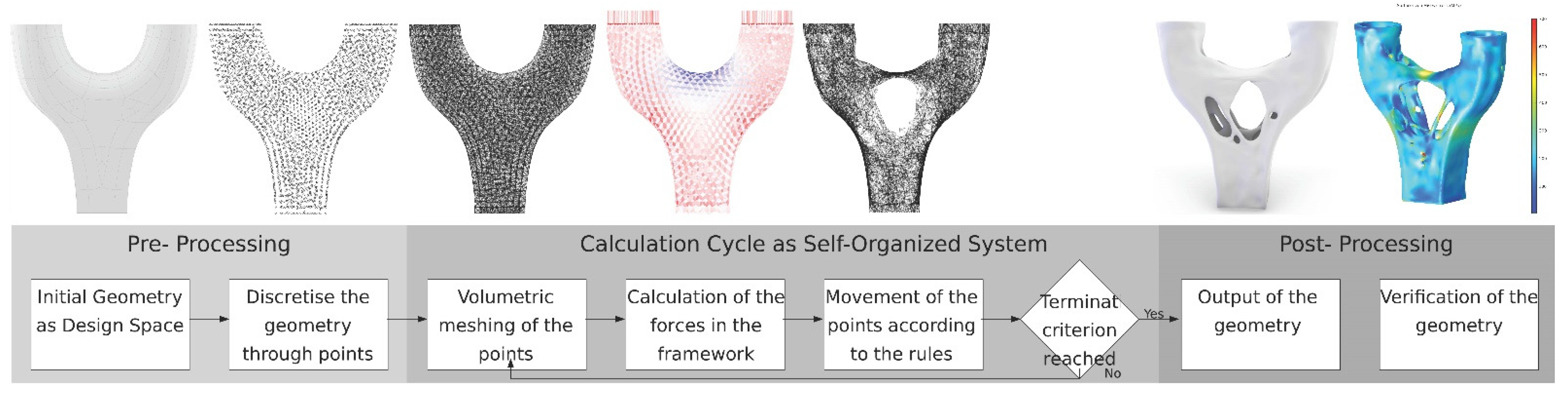
2.1. Self-Organizing System as Design Method for Structural Components

The term self-organizing system describes a system in which a global pattern or behavior is generated through the interaction of independent elements. It is used when the observation of a system consisting of many components reveals a pattern or internal order without an external controlling authority. It is rather the case that the observed behavior results from the interaction and collective behavior of the elements itself. A system described as self-organizing is one in which elements interact in order to achieve, dynamically, a global function or behavior [13] or, according to William Ross Ashby, each subsystem has adapted to the environment formed by all other subsystems [14].

Self-organizing systems are known from everyday life and observations without being explicitly classified as such for everyone. Typical examples are flocks of birds or fishes, the pattern that emerges when liquids are heated on one side, the behavior of insect colonies, or the interaction of neurons in the brain. The fact that self-organizing systems can also be used for optimization tasks can be seen in the example of ants finding their way to a food source. Initially, the ants swarm out in search of food. As soon as an ant has found something, it goes back to the anthill. On the way there, it leaves a pheromone trail. This trail points the way for other ants. The shorter the path, the more ants will choose this path and also leave a pheromone trail, while alternative longer paths are chosen less frequently. Due to the volatility of the pheromones, the best path is ultimately marked most strongly.

2.2. Application of a Self-Organized System for Force Flow Optimization

In order to apply the methodology of a self-organizing system for finding the shape of a geometry for additive manufacturing, some terms must be defined in advance. Because of the broad spectrum of applications of self-organizing systems, it is difficult to find a generally valid definition. For this paper, the following working definition by Camazine et al. is used:

“Self-organization is a process in which pattern at the global level of a system emerges solely from numerous interactions among the lower-level components of the system. Moreover, the rules specifying interactions among the system’s components are executed using only local information, without reference to the global pattern.”

[15] (p. 8)

The term self-organization already contains the concept of organization, which indicates an inner order or the goal of such an order. From the point of view of a force-flow-optimal material distribution within the design space for a given load case and a specific purpose, such as a node in steel construction, the material distribution in the base geometry corresponds to a highly disordered state. The material is equally distributed everywhere, regardless of how much it is utilized. If the design space is discretized in terms of points (for example, one point for each molecule), the result is an almost chaotic arrangement with no identifiable pattern. As a rule, however, mechanical considerations of components do not take place at the molecular level. With the transfer from the nanoscale to the microscale, the points can be regarded as the corner points of a partial volume. If the geometry is resolved as a tetrahedron mesh, the individual partial volume of the geometry is a single tetrahedron and the point is a vertex of this tetrahedron. The arrangement of the points can be arbitrary and chaotic, as long as the complete volume is filled. Self-organizing systems are often used to represent complex issues and models. Yet the concept of complexity is far less sharply defined than one might expect, and is repeatedly the subject of scientific work. A definition of complexity is not given in this paper, but some remarks should be made on this. Banzhaf notes:

“The treatment of chaotic systems has been derived from non-linear system theory. Chaotic systems are usually low-dimensional systems which are unpredictable, despite being deterministic. The reason being that the non-linear interaction among its components prohibits detailed analysis and prediction. Complex systems, on the other hand, have many degrees of freedom, mostly interacting in complicated ways. Complexity itself can be measured, notably there exist a number of complexity measures in computer science, but describing or measuring complexity is not enough to understand complex systems. The notion of emergence has been introduced in complex systems theory in order to explain the appearance of new qualitative features on the level of the entire system that where not present at the level of its components.”

[16] (pp. 10–11)

The complexity of a system is linked to emergence. While a system exhibits complex behavior on the macroscopic level, the individual participant can only show quite simple behavior on the microscopic level. This can be simplified according to Aristotle as the whole is more than the sum of its parts. This very simplified description of emergence already shows that there is a need for an observation on a micro and a macro level, as both are not independent of each other. With regard to emergence, there are different ways of looking at it, which are illuminated in an elaboration by Wolf and Holvoet [17] in relation to self-organizing systems. In the approach presented here, emergence can be seen as the pattern of points that is created in order to generate a geometry for additive manufacturing.

Also of importance is the point of view and purpose of the self-organizing system when interpreting the results. Atmanspacher [18] and Edmonds [19] show in their elaboration that the recognition and interpretation of complexity is strongly dependent on the viewpoint of the observer. The same applies to the interpretation of a pattern and its recognition. In the context of this work, an approach is adopted that considers the mechanical behavior of a geometry under the influence of force. With an increasing number of boundary conditions to be met, the complexity of the task to find a topology-optimized geometry, which meets all required boundary conditions, also increases. Only from this perspective is meaning assigned to the emergence of the system and interpreted accordingly.

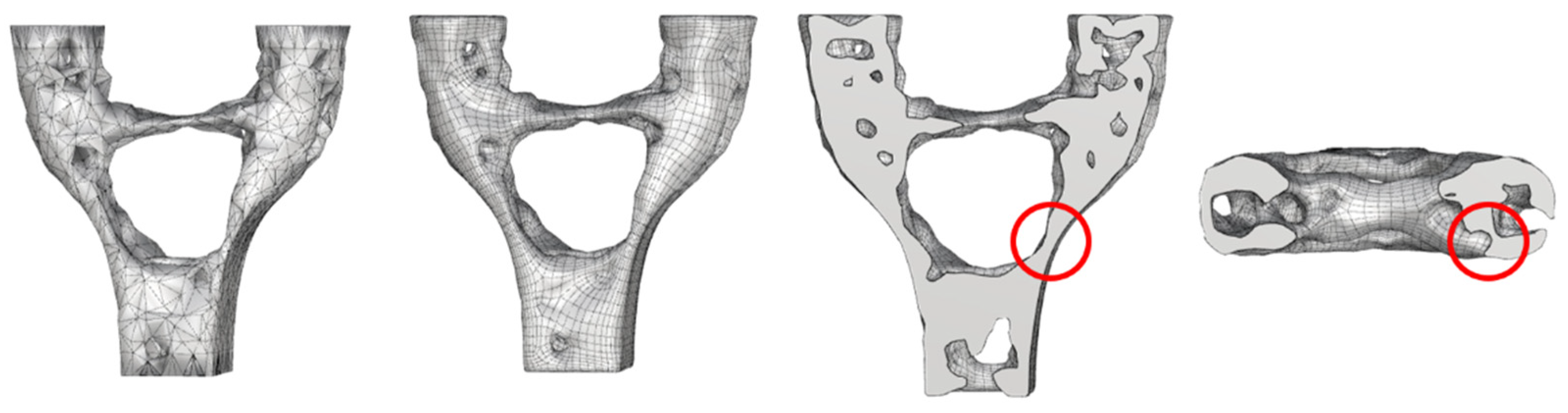
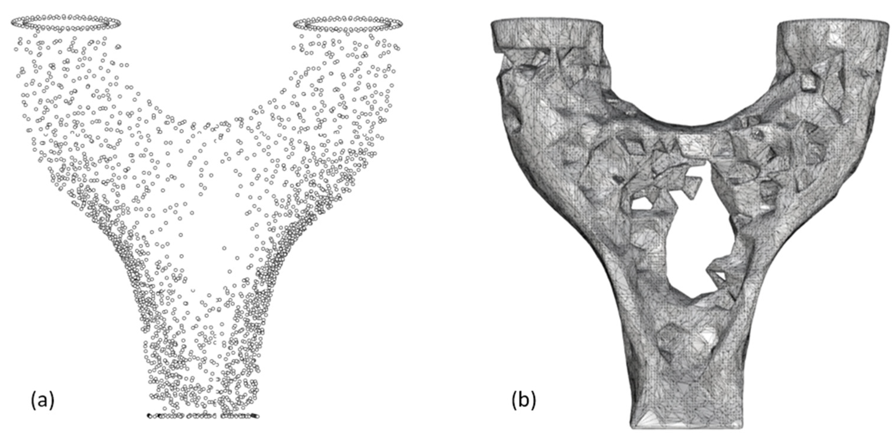
2.3. The Use of a Self-Organizing Systems to Find the Shape of a Topologically Optimized Node in Steel Construction

The process of creating a geometry for DED-arc takes place in several steps. The goal is an efficient material utilization and compliance with the restrictions regarding manufacturing. The individual steps of geometry generation via self-organizing systems are explained in more detail below. A schematic graphical representation of the design process is shown in Figure 5.

In terms of finding the shape of a geometry under a specific load case, the initial state is the design space. The design space limits the movement of the points and thus represents the first means of giving the geometry a predefined shape. The creation of the initial geometry is therefore the step where the architectural design is defined. In the variant presented here, the volume of the initial geometry later serves as a reference for the targeted termination criterion of the iteration cycle.

After creating the initial geometry as a volume, it is populated with points that are as evenly distributed as possible. The self-organizing system used here is based on these points. They serve as agents of the self-organizing system, which is a reason the approach presented in this paper is dealing with an agent-based model (ABM). The point itself is very simple in this consideration and only contains its position in space. In a further step, rules are applied to this point via iteration cycle. The behavior of the point as a single agent in the system is defined by the rules, which apply to all points. This leads to a movement of the points and thus to a change in their position in space.

In the next step, the points are volumetrically meshed with each other. This step leads to a definition of the neighborhoods of the points among each other as shown in Figure 5, third graph from the left. At the same time, this step discretizes the volume of the initial geometry into individual tetrahedrons. The edges of the tetrahedron not only serve to define the neighborhoods of the individual points among each other, but also as a set of rods for calculating the flow of forces within the geometry. In order to be able to generate a change in the geometric topology on a macroscopic scale, a mechanism is implemented here that removes tetrahedrons with an edge length that is too long from the volumetric network.

In the mechanical calculation step, the edges of the tetrahedrons are assumed to be members of a framework. Starting from the initial geometry, the mechanical boundary conditions are defined. These include individual points as load application points and points that serve as supports. In this example, it is a Y-node with load from above and restraint at the base as shown in the middle diagram of Figure 5. The red and blue colored areas represent the utilization of the individual members of the framework. This step is used to calculate the load from a continuous stress field in a geometry, defined as a volume, to a calculation of bar forces of a discrete representation of the initial geometry. Through this simplification, it is possible to apply a self-organizing system as a problem on a graph with a heuristic solution. At the same time, however, this simplification leads to a reduction in the accuracy of the calculation of the force flow.

With the calculation results of the previous step, rules for the behavior and interaction of the points are established. A distinction can be made between rules that cause the points to move and rules that restrict or prevent the points from moving. As an example, a movement rule for force flow optimization is presented here. A greedy heuristic is used for the force-flow optimization. For this purpose, a ranking of the sensitivity numbers of all neighboring points of a considered point is created. From this ranking, the neighboring point with the highest sensitivity value is taken as the direction if this sensitivity value is greater than that of the currently considered point. Otherwise, the point remains where it is. The sensitivity number is based on the elastic strain energy of the bars of the framework and is, in the basic form, calculated for each bar as follows:

$${\alpha }_i^E=\frac{1}{2}{f}_i^2{l}_i$$

(1)

The element sensitivity of each bar element ${\alpha }_i^E$ results from the force$f_i$ in the bar and its length$l_i$. In the approach used here, the self-organizing system consists of points. For this reason, the sensitivity of the bar elements must be related to the points. For this, several steps are necessary, which includes both a filtering over neighboring points and an averaging with the sensitivities of the previous iteration step.

This leads to a behavior on the macro level in which a point concentration occurs in areas with a high load on the bars by reducing the edge length to this area. The following rules serve as an example for rules that restrict the movement of the points. Points on which loads are applied for the framework calculation and points that serve as support points are basically excluded from movements. There is also a limit value that ensures that points do not move too close together. This prevents the points from concentrating in only one place after several iterations.

In order to create a self-organizing system that generates a force-flow-optimized geometry as a pattern, a balance must be found between rules for the movement of the points and rules for the restriction of the movement of the points. The movement rule is designed in such a way that the system returns to a state that is equivalent to the original one when no forces are acting on the framework. This loss of emergence and reversion to a chaotic distribution with respect to a force flow optimized material distribution is a typical property of self-organizing systems.

The graph between the points, the calculation of the forces in the framework, and the movement of the points according to the heuristic is carried out iteratively until the termination criterion is reached. This iteration loop represents the self-organizing system in a narrower sense and is used to solve the following optimization problem:

$$inf C=\frac{1}{2}{f}^{t}u$$

(2)

$$s. t. V_t-{\sum }_{i=0}^N{V}_i=0$$

(3)

Here C is the average compliance resulting from the elastic strain energy of the system. With $V_t$ as the target volume and $V_i$ the individual partial volumes of the elements during the calculation, the objective function is given in (2). This function is solved heuristically with the given approach.

After completion of the iterative process, the geometry is available as a rough mesh. This must then be smoothed and transferred into a format suitable for additive manufacturing. The result of a complete calculation is shown as an example in the second illustration from the right in Figure 5.

To check the result, the geometry was transferred into a common FEA software and calculated linearly elastic with the assumed load. The counterplot (Figure 5 on the right) shows a good utilization of the material. However, at points such as fillets and transitions in the material thickness, overloads in the material become visible. There, the steel node would deform plastically. To avoid this, it would be advantageous to perform shape optimization after topology optimization to reduce stress peaks that may occur.

After the generation of a geometry by self-organizing systems, the consideration of manufacturing restrictions, which strongly depend on the used set-up and software, is a step that needs to be undertaken. The approach for the identification and implementation of such restrictions is described in the following section.

2.4. Approach Description

A general description for the creation of the geometry and the execution of the path planning was given in the previous sections. There is a direct dependency between the presented aspects as shown schematically in Figure 6. For this reason, the interactions and how the dependencies were resolved are illustrated below using a node geometry as an example. The most obvious constraint results from the manufacturing setting itself. This can be seen in the example of the overhang. Depending on the degrees of freedom of the robotic production system and the presence of a tilt/turn-table, there is a different limit for the overhang. In particular, the tilt/turn-table as an additional axis reduces restrictions with regard to the overhang to such an extent that in the end it no longer has any significance.

To determine the limitations of DED-arc manufacturing in terms of geometry, the following approach was selected. A Y-node was force-flow optimized under a representative load. The force-flow-optimized node fulfils exclusively mechanical requirements. The resulting geometry was examined with regard to manufacturing possibilities. For this purpose, individual parts or structures of the node were cut out as a Case Study Demonstrator. Subsequently, it was investigated how this Case Study Demonstrator can be manufactured and where the manufacturing limits are. The general workflow is given in Figure 7.

After obtaining the optimized geometry of the steel node to be produced, the model needs to be transferred to the manufacturing planning. A slicing must be conducted and strategies for the manufacturing with regard to the manufacturing system need to be identified, both for the single layers and the whole structure.

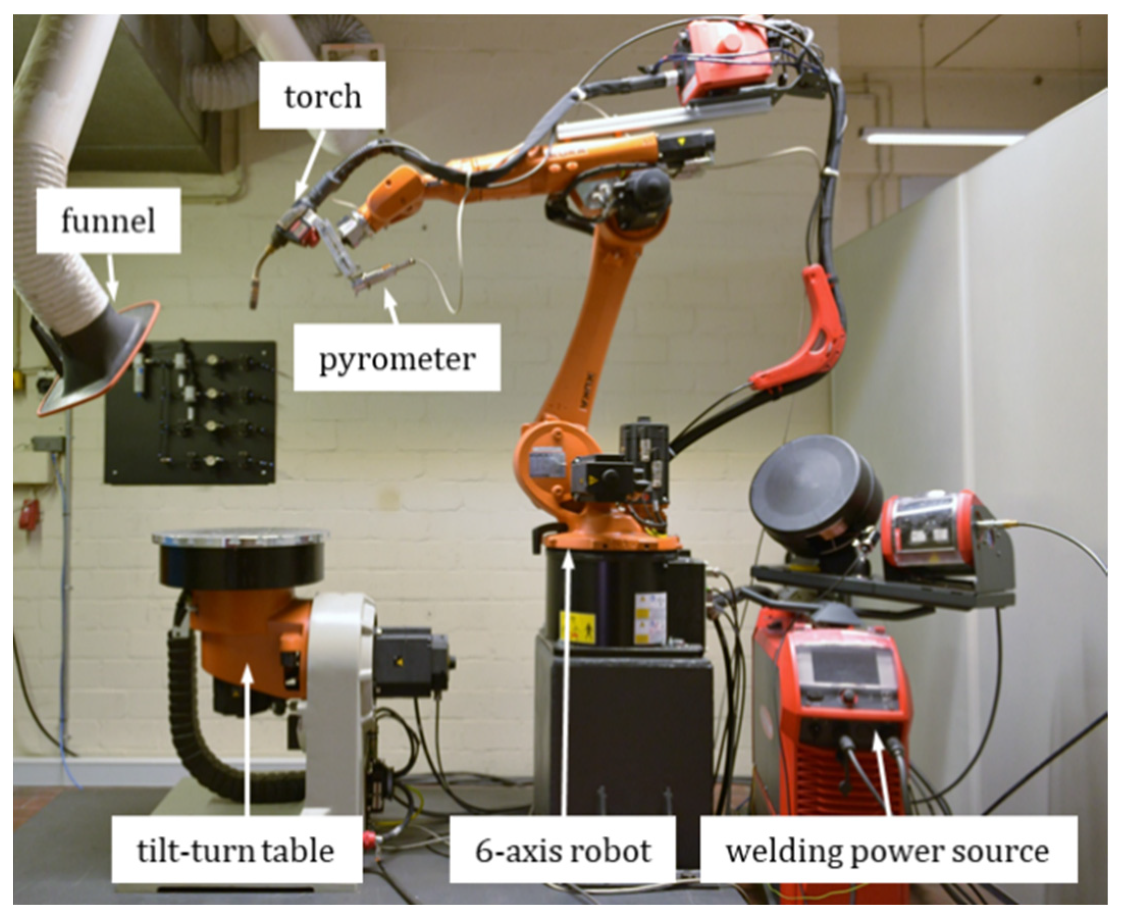
2.5. Wire Arc Additive Manufacturing

The experimental setup for the manufacturing of the Case Study Demonstrator consists of a KUKA KR-22 6-axis robotic system with a tilt/turn positioning table, coupled with a Fronius TPS500i welding power source, Figure 8. For the path planning and the subsequent generation of the robot program, the software DCAM CAD/CAM by SKM Informatik was used.

The Case Study Demonstrator used for the identification of manufacturing restraints is depicted in Figure 9. It is a cutout of the optimized steel node containing different geometrical features. One of the two features that are investigated more closely is the change of the wall thickness, with respect to the minimum wall thickness. The other one is the overhang, which is, due to the building strategy and the wall thickness close to the undercut, an overhang parallel to the welding direction. The layer height was, based on previous investigations, set to 2.2 mm. Despite the presence of a tilt/turn-table, these restraints were only identified for 3-axis manufacturing.

Table 1. Process parameters for the sample manufacturing.

Parameter	Value
Average Current	110 A
Average Voltage	14.9 V
Wire feed speed	3 m/min
Welding speed	45 cm/min
Average energy input per unit length	2.1 kJ/cm
Interpass temperature	200 °C

provides an overview of the process parameters. The applied characteristic curve was CMT Dynamic. The average current ${\overline{I}}_i$ and voltage ${\overline{U}}_i$ were obtained from process monitoring using a HKS WeldScanner with a sample rate of 1 kHz. As shielding gas, M21 was used, with a composition of 18% CO₂ and 82% Argon. The flow rate was 16 L/min. Further, the contact tip to workpiece distance was set to 15 mm. In general, it can be said that an adjustment of the parameters leads to the fact that with increasing energy input, the beads become wider and the melt pool larger. This leads to larger minimum wall thicknesses and smaller maximum realizable overhangs.

As a fabrication strategy/build up pattern, the raster pattern was chosen (compare Figure 3a), as it showed the best results regarding lack of fusion. A contour path was added to the infill, as that provides a better surface of the resulting part. The fabrication strategy of a representative layer is shown in Figure 10.

3. Results

3.1. Initial Design of Nodal Connector

As described in Section 2.3, a force-flow optimized geometry was created in the first step. The geometry is depicted in Figure 11. The load on these Y-nodes is one compressive force per branch. At the base point, the node is assumed to be rigid. The calculation was made with 2250 points as a self-organising system. The other key data of the calculation are given in

Table 2. Parameter of the geometry finding process.

Parameter	Value
Points	2501
Bars as elements	17,000
Iteration	312
Volume-Fraction	0.3
Mean compliance C	0.00218 kNm

. It can be seen that the geometry has different thicknesses over the height as well as the depth. However, due to the DED-arc method, a geometric minimum thickness needs to be maintained (red circles in Figure 11).

The originally created mesh-based geometry had to be transformed into a cleaned-up closed geometry in several steps. This was performed by transforming the triangular mesh of the surface into a quad-mesh by a marching cube algorithm with subsequent quad meshing. Both are included in the Grasshopper extension of Rhinocerus 3D. During this transformation, the mesh is slightly changed, which has led to a change in the wall thicknesses within the geometries. It should also be mentioned that the influence of the element size on the results has not been studied so far.

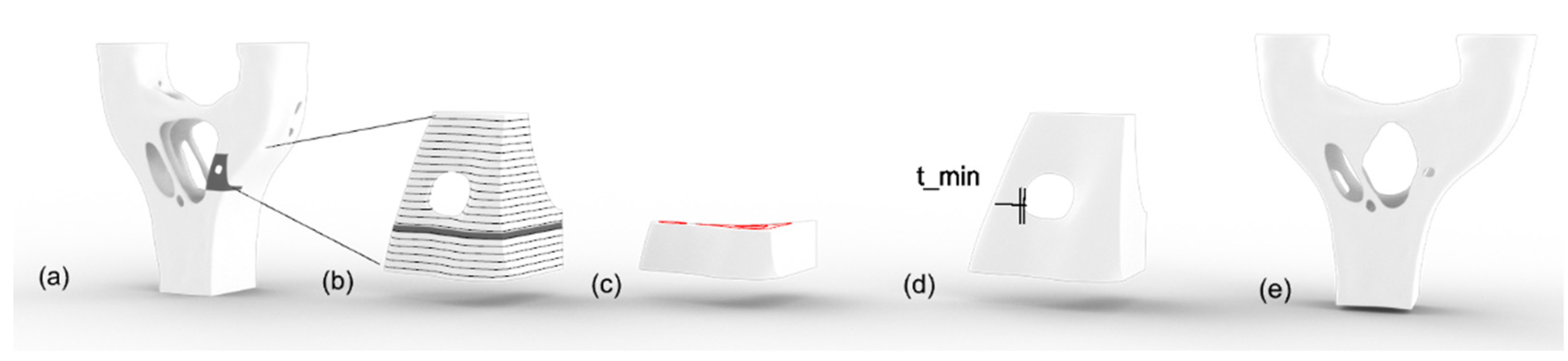
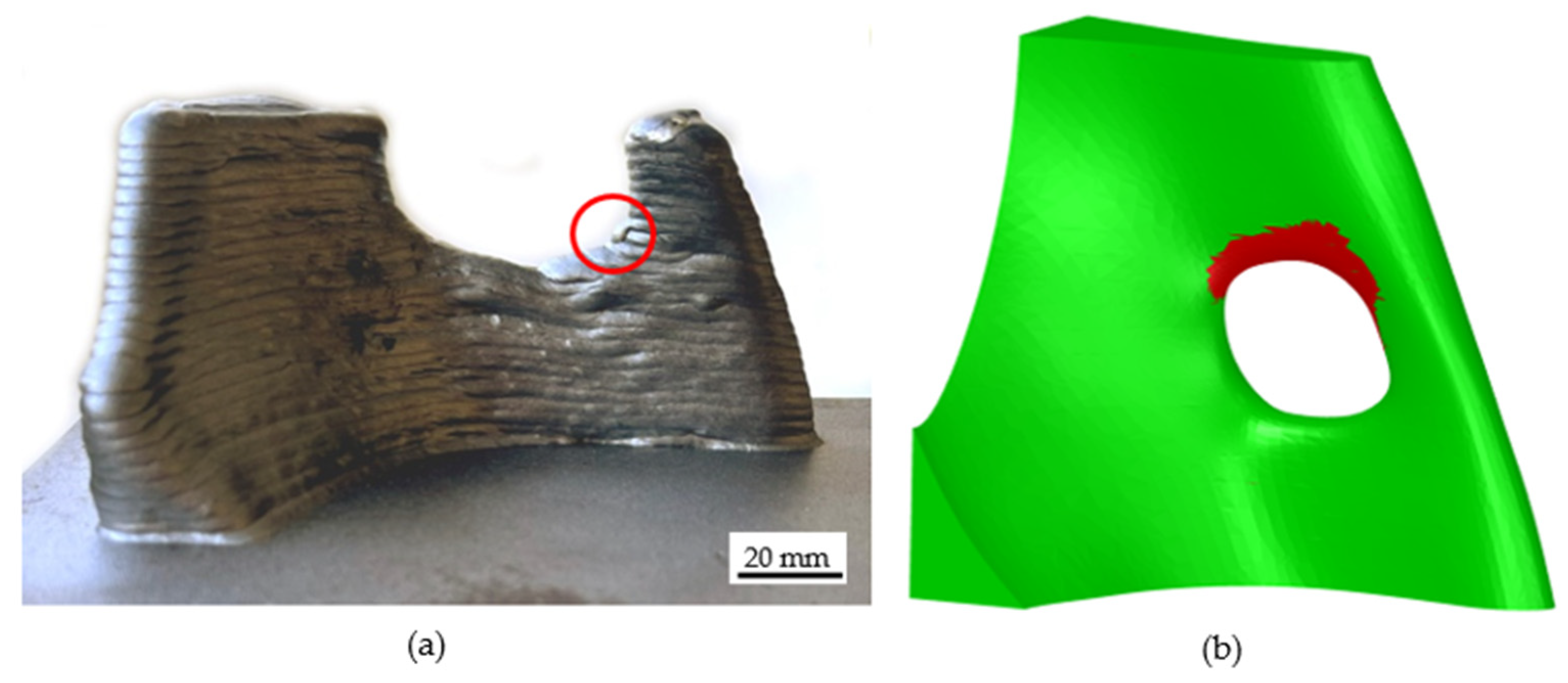
3.2. Deriving Manufacturing Restraints by the Fabrication of a Representative Detail of a Force Flow Structure

For the initial implementation of manufacturing restraints in the design process, two characteristics where investigated. The first one is the minimal wall thickness and the second is the maximum overhang.

3.2.1. Minimal Wall Thickness

When generating a force-flow optimized structure, the wall width may be reduced in some areas which carry less load. Considering the manufacturing process of DED-arc, there is a limit, which depends on the width of a single weld bead. That means it is also dependent on the welding parameters. Furthermore, it is affected by the fabrication strategy for the layer, particularly the presence of a contour path. When applying a contour path, the minimum width would be the width of two weld beads minus the overlap.

For the applied welding parameters and the chosen build-up strategy, the minimum wall thickness was determined to 9 mm, as shown in Figure 12. By the consideration of this restraint during the design process of the force-flow optimized structure, the generated mesh will be reordered. This enables a better material utilization and of course, a better shape accuracy.

3.2.2. Overhang Parallel to Welding Direction

There are two different types of overhangs. The first one would be the overhang that is perpendicular to the welding direction. In this case, bigger overhangs (up to 90°) are possible. When welding an overhang parallel to the welding direction, for example as it occurs for the undercut in the Case Study Demonstrator, the maximum overhang is much lower. The reason for that is described in [20]. For the overhang parallel to the welding direction, there is not enough support material, and thus the torch is missing the previous welded layer. Figure 13 shows the limit of the overhang parallel to the welding direction. For the used parameter set and a 3-axis manufacturing approach, the maximum is at 18°. This was identified by the formation of droplets when welding the layer with an overhang to the previous layer of higher than 18°. The overhang analysis (Figure 13b) shows all areas with a critical overhang (red).

By considering the maximum overhang in the welding direction during the design, the undercuts would be modified and the upper part of it would taper with an overhang of smaller than 18°.

3.3. Iteration of Initial Design Considering Manufacturing Restraints

In the previous section, it was shown which manufacturing constraints could be determined using the Case Study Demonstrator. In addition to the overhang as an abort criterion, the minimum thickness of the component was also determined. This must be taken into account when generating the geometry. For this purpose, a behavior rule was created for the agents of the self-organizing system that guarantees the minimum thickness at every point of the component.

The rule is illustrated in Figure 14a. Each point of the surface mesh is considered individually. Starting from this point, all neighboring points within the distance with the length of the minimum thickness of the geometry are selected. Then all the faces of the surface mesh that belong to the previously selected points are collected. Next, the surface normal of these individual faces are placed in the point of interest and a ray is constructed for each normal. For each ray it is examined whether there is an intersection point with the geometry and, if so, how far away it is. If the distance is less than the minimum thickness, the point under consideration is transposed along the corresponding ray so that the distance to the intersection point with the geometry is equal to the minimum thickness. The parameters for the thickness rule are listed in

Table 3. Parameter of the geometry finding process with thickness rule.

Parameter	Value
Points	2501
Bars as elements	17,000
Iteration	312
Volume-fraction	0.3
Mean compliance C	0.00208 kNm
Min. thickness	12.5 mm

.

The result of applying the minimum thickness rule can be seen in Figure 15. The same node as in Figure 11 is shown after the force flow optimization, but with an additional behavior rule for the points. It can be seen in the red circled areas that the thickness of the structure is higher than in the initial geometry. This also leads to a change in the geometry of the structure. The topology has changed and there are larger holes and openings.

In addition to the rule for maintaining the minimum thickness, Figure 14b schematically shows the approach of a rule intended to limit the overhang within the structure. Again, the normal of each triangle of the surface mesh is used as a reference. Based on the angle of the surface normal, the lowest vertices of the considered triangle surface can then be selected and rotated around the uppermost one, so that the surface normal has a maximum overhang angle +90° to the vertical. The additional 90° result from the vertical as a reference, which results from the production direction with respect to gravity. This rule is applied to all vertices belonging to a face with a downward pointing surface normal.

In Figure 16a, it can be seen that the agents of the self-organizing system move further and further downwards due to the overhang rule. This is caused by the direction of movement, since the compensation of the overhang is carried out by a downward rotation. The result is a lower concentration of agents in the upper part of the geometry, which next leads to gaps and defects when the points are connected.

4. Conclusions and Recommendation

In the work presented here, it was shown that there is a direct connection between the design of a component for additive manufacturing using DED-arc and the manufacturing restrictions. In the first investigation, a geometry was generated using a new optimization approach. This approach aims to generate a geometry that is optimized for force flow and takes additional geometric constraints into account that are easy to implement. This is achieved by reducing the optimization problem to the question of the position of points in space. By considering the optimization task as a self-organizing system, additional constraints can be applied to the optimization. It is possible to directly access the position of the points on the surface which themselves define the shape of the geometry.

In addition, a Case Study Demonstrator was used to investigate which geometric constraints can occur in the manufacturing process with DED-arc. As an example, the minimum thickness of a component and the limitation of the overhang within the structure could be identified. It could be shown that it is possible to comply with the minimum thickness in all cross-sectional areas with the presented method. In contrast, compliance with the overhang rule could not be sufficiently applied because the geometry does not have a closed surface and therefore cannot be used. There is still a need to integrate this into the system.

To sum up the following conclusions could be drawn:

• It was shown that it is possible to create a mechanical optimized structure using self-organizing systems
• A method was presented where Case Study Demonstrators were used to investigate manufacturing issues. It was possible to determine the restrictions that the geometry must comply with in order to be producible for additive manufacturing by DED-arc.
• It was shown that with the presented method for generating the geometry, geometrical boundary conditions, such as the minimum thickness of the geometry, could be taken into account.
• Further boundary conditions such as the limitation of the overhang could not yet be successfully implemented with the presented method and are therefore still subject of research.

References

1. Buchanan, C.; Gardner, L. Metal 3D printing in construction: A review of methods, research, applications, opportunities and challenges. Eng. Struct. 2019, 180, 332–348. [Google Scholar] [CrossRef]
2. Ding, D.; Pan, Z.; Cuiuri, D.; Li, H. Wire-feed additive manufacturing of metal components: Technologies, developments and future interests. Int. J. Adv. Manuf. Technol. 2015, 81, 465–481. [Google Scholar] [CrossRef]
3. DebRoy, T.; Wei, H.L.; Zuback, J.S.; Mukherjee, T.; Elmer, J.W.; Milewski, J.O.; Beese, A.M.; Wilson-Heid, A.; De, A.; Zhang, W. Additive manufacturing of metallic components—Process, structure and properties. Prog. Mater. Sci. 2018, 92, 112–224. [Google Scholar] [CrossRef]
4. Ding, D.; Shen, C.; Pan, Z.; Cuiuri, D.; Li, H.; Larkin, N.; van Duin, S. Towards an automated robotic arc-welding-based additive manufacturing system from CAD to finished part. Comput.-Aided Des. 2016, 73, 66–75. [Google Scholar] [CrossRef] [Green Version]
5. Feucht, T.; Lange, J.; Erven, M. 3-D-Printing with Steel: Additive Manufacturing of Connection Elements and Beam Reinforcements. ce/papers 2019, 3, 343–348. [Google Scholar] [CrossRef]
6. Reimann, J.; Henckell, P.; Ali, Y.; Hammer, S.; Rauch, A.; Hildebrand, J.; Bergmann, J.P. Production of Topology-optimised Structural Nodes Using Arc-based, Additive Manufacturing with GMAW Welding Process. J. Civ. Eng. Constr. 2021, 10, 101–107. [Google Scholar] [CrossRef]
7. Rafieazad, M.; Ghaffari, M.; Vahedi Nemani, A.; Nasiri, A. Microstructural evolution and mechanical properties of a low-carbon low-alloy steel produced by wire arc additive manufacturing. Int. J. Adv. Manuf. Technol. 2019, 105, 2121–2134. [Google Scholar] [CrossRef]
8. Bourlet, C.; Zimmer-Chevret, S.; Pesci, R.; Bigot, R.; Robineau, A.; Scandella, F. Microstructure and mechanical properties of high strength steel deposits obtained by Wire-Arc Additive Manufacturing. J. Mater. Process. Technol. 2020, 285, 116759. [Google Scholar] [CrossRef]
9. Rodrigues, T.A.; Duarte, V.; Avila, J.A.; Santos, T.G.; Miranda, R.M.; Oliveira, J.P. Wire and arc additive manufacturing of HSLA steel: Effect of thermal cycles on microstructure and mechanical properties. Addit. Manuf. 2019, 27, 440–450. [Google Scholar] [CrossRef]
10. Michel, F.; Lockett, H.; Ding, J.; Martina, F.; Marinelli, G.; Williams, S. A modular path planning solution for Wire + Arc Additive Manufacturing. Robot. Comput.-Integr. Manuf. 2019, 60, 1–11. [Google Scholar] [CrossRef]
11. Ding, D.; Pan, Z.; Cuiuri, D.; Li, H. A practical path planning methodology for wire and arc additive manufacturing of thin-walled structures. Robot. Comput.-Integr. Manuf. 2015, 34, 8–19. [Google Scholar] [CrossRef] [Green Version]
12. Blum, H. A Transformation for Extracting New Descriptions of Shape; MIT Press: Cambridge, MA, USA, 1967; pp. 362–380. [Google Scholar]
13. Gershenson, C. A General Methodology for Designing Self-Organizing Systems. ECCO Work. Pap. 2005. [Google Scholar] [CrossRef]
14. ASHBY, W.R. Principles of the self-organizing dynamic system. J. Gen. Psychol. 1947, 37, 125–128. [Google Scholar] [CrossRef] [PubMed]
15. Camazine, S.; Bonabeau, E.; Deneubourg, J.-L.; Franks, N.R.; Theraula, G. Self-Organization in Biological Systems; Princeton University Press: Princeton, NJ, USA, 2001; ISBN 0691212929. [Google Scholar]
16. Banzhaf, W. Self-organizing Systems. In Encyclopedia of Complexity and Systems Science; Springer: New York, NY, USA, 2009; pp. 8040–8050. [Google Scholar] [CrossRef]
17. de Wolf, T.; Holvoet, T. Emergence Versus Self-Organisation: Different Concepts but Promising When Combined. In Engineering Self-Organising Systems; Hutchison, D., Kanade, T., Kittler, J., Kleinberg, J.M., Mattern, F., Mitchell, J.C., Naor, M., Nierstrasz, O., Pandu Rangan, C., Steffen, B., et al., Eds.; Springer: Berlin/Heidelberg, Germany, 2005; pp. 1–15. ISBN 978-3-540-26180-3. [Google Scholar]
18. Atmanspacher, H. On Macrostates in Complex Multi-Scale Systems. Entropy 2016, 18, 426. [Google Scholar] [CrossRef] [Green Version]
19. Edmonds, B. Complexity and Scientific Modelling. Found. Sci. 2000, 5, 379–390. [Google Scholar] [CrossRef]
20. Plangger, J.; Schabhüttl, P.; Vuherer, T.; Enzinger, N. CMT Additive Manufacturing of a High Strength Steel Alloy for Application in Crane Construction. Metals 2019, 9, 650. [Google Scholar] [CrossRef]
Figure 1. Development of relative work productivity per worker in Germany since 1991 (100%), data taken from [1].
Buildings 12 02154 g001
Figure 2. Flowchart of the MPP method: layer segmentation, path planning, and zoning, by Michel et al. [10].
Buildings 12 02154 g002
Figure 3. Schematic of different build-up patterns: (a) raster, (b) zigzag, (c) contour and (d) spiral.
Buildings 12 02154 g003
Figure 4. Schematic for the generation of the medial axis, by [11].
Buildings 12 02154 g004
Figure 5. Presentation of the basic process of form finding. From left: Initial design as design space; point representation of the geometry; volumetric mesh of the point representation; calculation of the bar forces by means of FEA; volumetric mesh as result of the calculation cycle; output geometry as volumetric model; verified geometry on FEA model.
Buildings 12 02154 g005
Figure 6. Dependencies between manufacturing setup, geometry generation and path planning.
Buildings 12 02154 g006
Figure 7. Exemplary representation of the process for finding the manufacturing restrictions for the DED-arc setting used (a) Initial design of the node, (b) cutout used as Case Study Demonstrator, (c) first 14 layers of the demonstrator with tool path, (d) location of the constraint “minimal wall thickness”, (e) optimized node.
Buildings 12 02154 g007
Figure 8. Experimental set-up.
Buildings 12 02154 g008
Figure 9. (a) Part to be manufactured for the identification of the constraints minimum wall thickness and maximum overhang for 3-axis manufacturing (b) generated robot path (first 24 layers) for a layer height of 2.2 mm with a raster + contour filling strategy.
Buildings 12 02154 g009
Figure 10. Robot path of the first layer of the Case Study Demonstrator.
Buildings 12 02154 g010
Figure 11. From left to right: tetrahedron-surface-mesh of the generated geometry, quad-mesh of the geometry, vertical section through the node and horizontal section through the node. The calculation was performed without an additional condition.
Buildings 12 02154 g011
Figure 12. Criterion of minimum wall thickness (a) obtained wall thickness (b) planned robot path.
Buildings 12 02154 g012
Figure 13. Criterion of overhang parallel to the welding direction: (a) result of a 3 axis manufacturing of the part with droplets forming at an overhang of 18° and (b) overhang analysis with a threshold of 18°.
Buildings 12 02154 g013
Figure 14. (a) graphical representation of the minimum thickness rule and (b) graphical representation of a rule to limit the overhang.
Buildings 12 02154 g014
Figure 15. (a) tetrahedron-surface-mesh of the generated geometry (b) quad-mesh of the geometry (c) vertical section through the node, (d) horizontal section through the node. The calculation was performed with the additional condition of minimum thickness of 12.5 mm.
Buildings 12 02154 g015
Figure 16. (a) Graphical representation of the points of the volumetric mesh as agents of the self-organizing system. (b) Representation of the geometry after an intermediate step for the transformation from triangle mesh to quad mesh.
Buildings 12 02154 g016