Investigative Study on Adaptive Thermal Comfort in Office Buildings with Evaporative Cooling Systems (ECS) under Dry Hot Climate

Abstract

Evaporative cooling systems (ECS) in buildings, which are driven by cleaner and more sustainable energy, had been widely applied in recent years especially for the dry hot regions in summer. In this study, an investigation was conducted for office buildings by using ECS in Urumqi (China) from July to August 2021. Through subjective survey and objective measurements, 577 initial questionnaires and measured data were obtained. Outcomes showed that the indoor expectative temperature (T_e) was received by 26.6 °C, 0.7 °C lower than neutral temperature (T_n). And the acceptable intervals for the 90% and 80% level were obtained at 27.1–28.9 °C and 26.4–30.3 °C, respectively. It appeared to possess a wider scope than that calculated by PMV algorithm, which further indicted that subjects have adapted to the local climate. Furthermore, the adjustment PMV models (ePMV, APMV) were found to have an effectively narrow gap comparing to the actual thermal sensation vote (TSV). The appropriate usage intervals of ePMV and APMV were quantified by T_op < 27.6 °C/T_op > 29.8 °C, 27.6 °C < T_op < 29.8 °C, respectively. These findings may provide reference values for the revision of local energy-saving standard to some extent.

1. Introduction

1.1. Research Motivation

With the acceleration process of China’s urbanization, building technology brings with it new threats. For instance, efficient urban construction loses sight of the trade-off relationships between energy demand and thermal comfort. A large amount of conventional energy is used at the expense of environmental protection [1,2,3,4]. For sake of creating a more comfortable indoor thermal environment, the heating, ventilation and air conditioning (HVAC) system consumed approximately 50% of the building energy in more than half a century when it was widely used [5]. Furthermore, the refrigerant in a is the key offender in environmental pollution. Therefore, the exploration of indoor thermal environments under the background of cleaner and sustainable energy is put on the agenda.

Evaporative cooling systems (ECS), which are characterized by energy conservation, environmental friendliness, high efficiency and economic benefits, have been widely considered in recent years. They are driven by dry air energy (the difference among wet and dry bulb air temperatures). Meanwhile, through the process of heat and humidity exchange between water and air cools the indoor temperature [6,7]. Due to the abundant resource of dry air energy in northwest of China, it is the most suitable area for the application of this system. It is also worth mentioning that ECS can save around 30–80% energy demand compared to conventional air-conditioned buildings based on refrigerants and with less pollution [8].

In accordance with the explanation from the American Society of Heating, Refrigeration and Air Conditioning Engineers (ASHRAE), thermal comfort is a psychological state in which occupants are satisfied with current physical environment [9]. Several influential global standards had been established for evaluating the indoor thermal environment through the efforts of generations, such as the ASHRAE Standard [9], ISO 7730 [10], EN 15251 [11], and CIBSE Guide [12], from which the thermal comfort study can be classified as static and adaptive approach. Fanger’s predicted mean vote (PMV) model is based on steady-state heat transfer theory that takes six body/environmental parameters into consideration [13]. However, it is found not to be an appropriate way of calculating the thermal comfort levels in ECS buildings, as it ignores the ability of occupants adapting to a specific regional climatic environment. The adaptive comfort approach, which focuses on the people–environment interaction and takes the occupants’ natural tendency to adapt to changes in the thermal environment as well as restoring their comfort into account, has been regarded as reasonable and accurate [14,15]. Therefore, it is imperative to conduct a complete field survey for ECS buildings considering various cultural settings, economic levels, and individual habits to establish an adaptive thermal comfort model.

1.2. Previous Studies

Multiple studies have been carried out to probe thermal comfort standards based on field investigations in recent years; the results are different from varying climatic characteristics, seasons, and indoor operating modes, shown as in

Table 1. Summary of previous thermal comfort studies with different modes.

Mode	Scholars	Location	Season	Type	Model	1 Tn (°C)	2 CTI (°C)
3 ECS	Tewari [16]	Jaipur	Summer	Office	7 TSV = 0.27 9 Top − 7.63	28.15	24.5–31.8
	Bravo [17]	Maracaibo	Summer	Dwelling	TSV = 0.295 10 Ta − 8.2834	28.08	-
4 AC	Fu [18]	Guangzhou	Summer	Office	8 MTSV = 0.301Top − 7.902	26.2	29.27
	Indraganti [19]	Tokyo	Summer	Office	TSV = 0.299Top − 8.109	27.1	-
	Wang [30]	Harbin	Winter	Office	TSV = 0.2746Ta − 5.4226	19.7	-
	Jiang [31]	Gansu	Winter	Classroom	TSV = 0.18Top − 2.56	14.2	12.6–16.9
	Hwang [20]	Taiwan	Summer	Classroom	TSV = 0.14 11 ET* − 3.76	24.7	24.2–29.3
5 NV	Fu [18]	Guangzhou	Winter	Office	MTSV = 0.157Top − 3.262	20.7	-
	Liu [21]	Turpan	Spring	Dwelling	MTSV = 0.232Top − 6.035	22.53	12.5–31.5
			Summer		MTSV = 0.349Top − 9.152	24.37
			Winter		MTSV = 0.114Top − 2.013	23.45
	Yu [22]	Shanghai	Summer	Dwelling	MTSV = 0.124Top − 3.145	25.4	18.5–32.2
			Winter		MTSV = 0.076Top − 1.273	16.8	5.6–28.0
	Zhou [28]	Hunan	Winter	Dwelling	MTSV = ln(Top −7.42) −0.07	11.4	7.5–15
	Zhang [23]	Guangzhou	Summer	Office	TSV = 0.256 12 SET* − 6.515	25.4	23.5–27.4
	Wu [29]	Guangzhou	Winter	Office	TSV = 0.2027Top − 4.7173	23.27	-
	Jiang [31]	Gansu	Winter	Classroom	TSV = 0.14Top − 1.95	13.9	14.8–17.7
6 MM	Tse [24]	Cardiff	Summer	Office	TSV = 0.2203Top − 4.2482	19.3	14.7–23.8
			Winter		TSV = 0.2181Top − 3.6769	16.9	12.3–21.4
	Ming [25]	Chongqing	Spring	Office	TSV = 0.22Top − 5.77	26.23	23.0–28.0
			Summer		TSV = 0.29Top − 7.59	26.17	24.7–29.0
			Autumn		TSV = 0.27Top − 6.96	25.78	22.0–28.8
	Wu [26]	Changsha	Summer	Office	TSV = 0.18Top − 4.86	27.0	24.2–28.4
	Martin [27]	Seville	All	Office	MTSV = 0.17Top − 4.33	25.47	-

Note: ¹ neutral (comfort) temperature; ² comfort temperature interval; ³ evaporative cooling system; ⁴ air-conditioned buildings; ⁵ naturally ventilated buildings; ⁶ mixed mode buildings; ⁷ thermal sensation vote; ⁸ mean thermal sensation vote; ⁹ operating temperature; ¹⁰ indoor air temperature; ¹¹ new effective temperature; ¹² standard effective temperature.

. In summer, it can be found that the neutral temperature (T_c) for all locations is in the range of 24.0–29.0 °C regardless of indoor working conditions [16,17,18,19,20,21,22,23,24,25,26,27], except in Cardiff, which is relatively low [24]. The reason is mainly due to the indoor setting temperature of this region being lower than in other sites. As for winter, T_c is roughly distributed between 16.0–24.0 °C, which is lower than in summer [18,21,22,24,27,28,29,30,31]. Among them, only the studies in northwest China [21] and Hunan [28] are out of range, leading the T_c with less than 14.5 °C. The reasonable explanation is that extreme local climate has affected human thermal adaptation. In addition, there are basically two types of thermal comfort models in previous studies: Fanger’s PMV/PPD models with static conditions and adaptive models with dynamic conditions. However, the outcomes indicated that the authentic thermal sensation may go beyond the predicted range provided by the ASHRAE Standard [9], EN 15251 [11] which is based on the PMV model. For example, field studies were conducted for AC office buildings [18,19] and classrooms [20] located in different climatic zones during the summer season, and results reported that the neutral temperatures were different from ASHRAE Standard with the PMV model always significantly overestimating the actual thermal sensation due to the wider range of adaptations by subjects. Comparing another group of NV office buildings in Guangzhou [29], although nearly half of the measured data exceed beyond the comfort zone from ASHRAE, most of them are still distributed in an acceptable range based the on adaptive model. Furthermore, J. Tse [24], R. Ming [25], and E. Martin [27] were all focusing on MM office buildings to explore the thermal adaption in different seasons, and jointly pointed out that owing to occupants being more sensitive to environmental changes, a wider range of acceptability on the part of themselves in buildings exists.

Evaporative cooling systems are becoming increasingly prevalent in the office buildings of China to ensure indoor thermal comfort during summer season [32,33]. This study is significant because with the massive application of cleaner energy sources, indoor thermal environments created by ECS are quite different from the conventional working modes, such as NV, AC, and MM buildings. The main reason is it can provide occupants with both a physical approach (such as operating windows flexibility) and mechanical cooling systems [16]. Moreover, exploring the ECS adaptive model can also reduce unnecessary energy usage to a large extent, so as to reach the “Double Carbon” target set by the Chinese government. Unfortunately, there are hardly any elaborate field studies on thermal comfort implemented in ECS office buildings in China. Meanwhile, the adaptive models for the prediction of thermal comfort are not yet established, which means the cooling load required for such buildings in summer cannot be accurately gained. Therefore, only by gathering sufficient information from field investigation can an in-depth quantitative analysis be obtained. Through quantitating the optimal interval of the predicted model by former researchers, the relationships between thermal comfort and environmental indexes can be systematically summarized to fill in the gaps for correlational research. The innovation of the present study is the first attempt to adopt field investigations, subjective responses, and objective measurements for exploring occupants’ thermal sensations and adaptive models in ECS office buildings in China. Moreover, the optimal interval of adjustment of PMV models based on a steady-state condition is also quantified to compare with the adaptive model. It may provide a new ideas for improving the accuracy of thermal evaluation.

1.3. Purpose of the Study

With the issues mentioned above, the purpose of this paper mainly lies upon five points as follows:

(1)

To probe the authentic indoor physical environment and thermal comfort in office buildings by using ECS in Urumqi during the summer season.

(2)

To determine the neutral (comfort) temperature, expectative temperature, and acceptable temperature ranges for these office subjects.

(3)

To establish an adaptive model of human sensation in consideration of the specific dry hot climatic condition.

(4)

To search the appropriate usage intervals of adjustment-predicted models for ECS office buildings in Urumqi.

(5)

To analyze the differences between the adaptive model and different working modes using previous studies.

2. Methodology

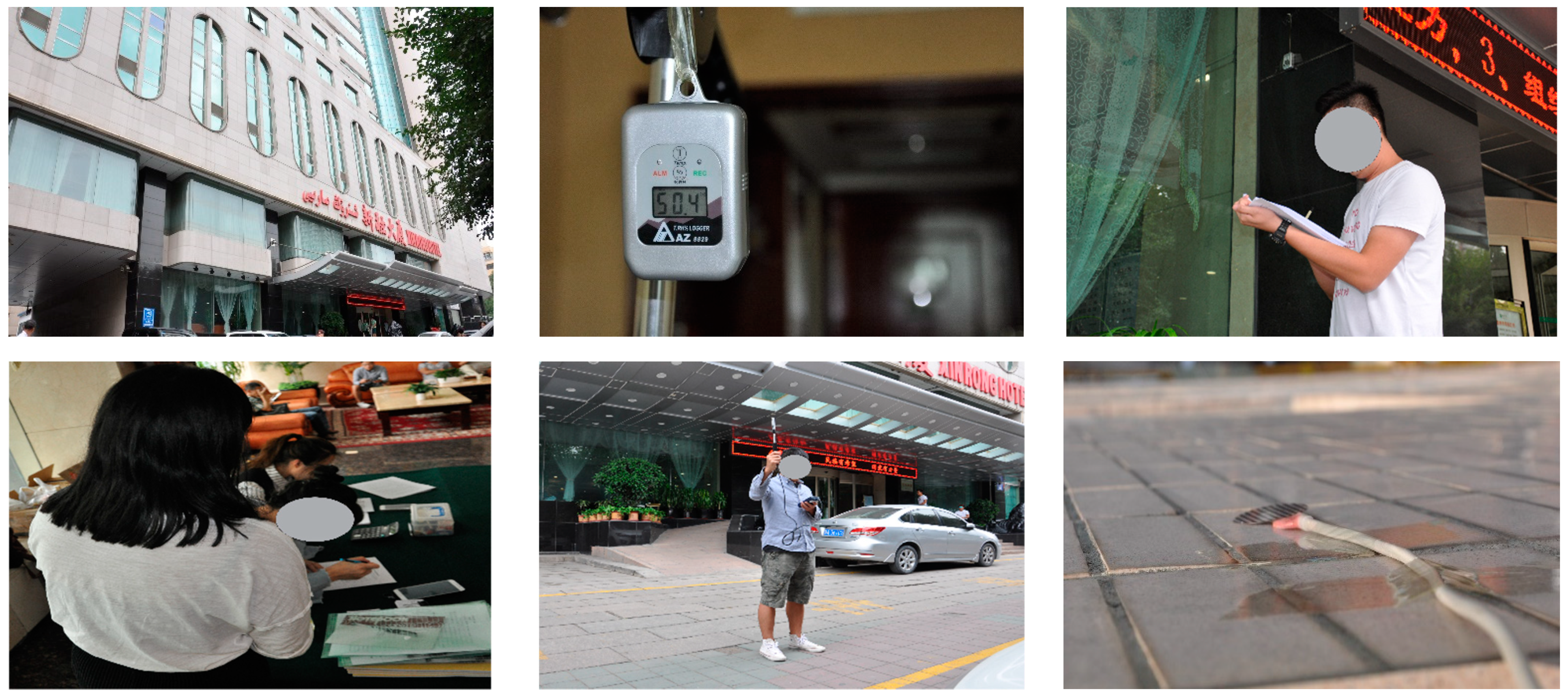
2.1. Overview of the Investigation

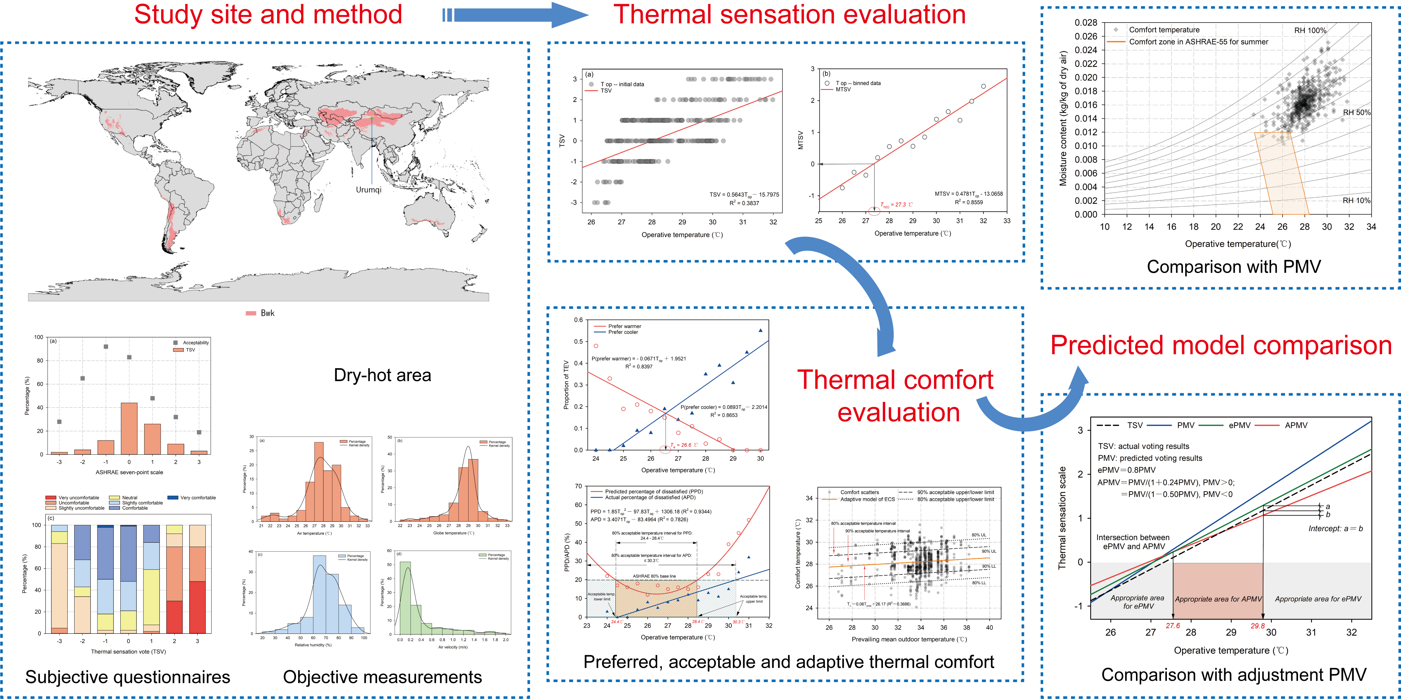
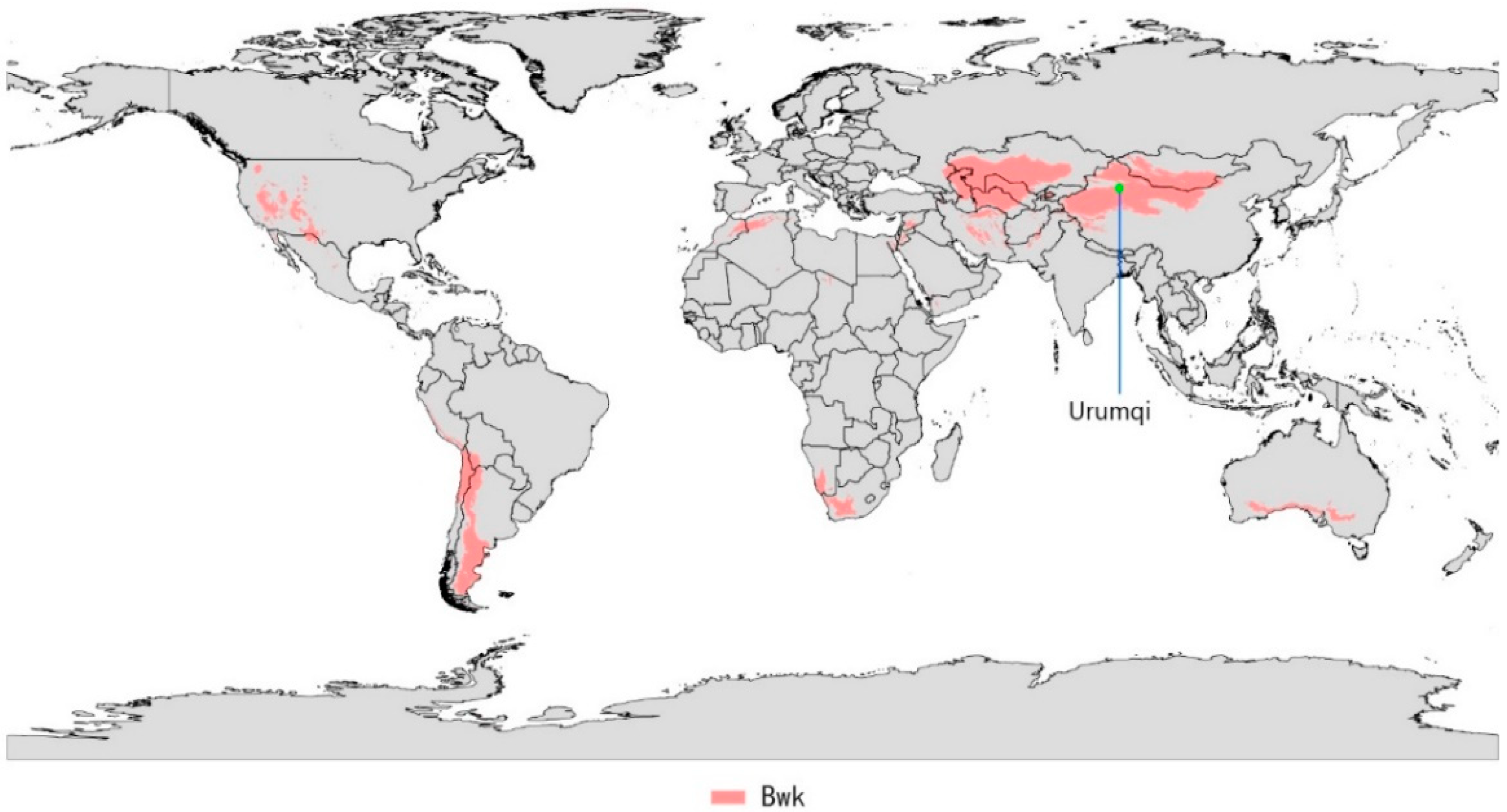
2.1.1. Location and Regional Climatic Conditions

The survey site of this study is in Urumqi, the capital of Xinjiang autonomous region, which is located in the northwest of China (latitude: 43.47° N, longitude: 87.37° E and elevation: 917.9 m above mean sea level) [34]. Based on the Köppen–Geiger climate classification, Urumqi can be classified as a cold desert climate zone (Bwk) [35], with a dry hot characteristic in summer and dry cold in winter, as shown in Figure 1. The hottest period throughout the year is from June to August with maximum outdoor temperature of up to 38.4 °C. The coldest period is from December to February with a minimum temperature of up to −12.6 °C (Figure 2). The maximum difference between outdoor wet and dry bulb air temperature in summer can reach approximately by 15.7 °C. Meanwhile, due to the intense solar radiation and sparse precipitation (less than 200 mm/year), Urumqi experiences a dry hot climate in summer with lower relative humidity which the mean value roughly equal to 45.5%. Therefore, the insufficient moisture in the atmosphere throughout the year, especially in summer, can lead to thermal discomfort (such as dehydration) due to the higher skin evaporation.

2.1.2. Target Building Characteristics

The 8 surveyed office buildings in this study were all located within 6 km of the Urumqi central area. Meanwhile, the main principle of the selected testing space was as follows: (1) there should be similarity or consistency in the use of new energy systems (refer to ECS); (2) the occupants’ usage rate should be as high as possible so as to minimize the accidental error of measuring results; (3) the indoor thermal environment indexes required by subjects are in substantial agreement. Additionally, the heat transfer coefficient (U-value) of these buildings (roof and exterior wall) can be calculated by thermal physical property parameters of each layer material [36]. In addition, surveyed buildings were both equipped with direct evaporate cooling systems, and the specific pattern was the combination of evaporative cooling high temperature chillers, evaporative cooling fresh air processors and terminals (fan coils).

Table 2. Description of the surveyed office buildings.

No.	Age	Wall		Roof		Window
		Construction	U-Value W/(m2·K)	Construction	U-Value W/(m2·K)	Construction	U-Value W/(m2·K)	SHGC
01	6	-	-	Poured concrete	0.24	Double glazing with vacuum layer	1.8	0.6
02	9	Steel-framed concrete	0.32	Poured concrete	0.24	Double glazing with vacuum layer	1.8	0.5
03	10	-	-	Poured concrete	0.24	Double glazing with vacuum layer	2	0.6
04	15	Double brick	0.35	Cement and asbestos sheet	0.24	Double glazing with vacuum layer	1.8	0.65
05	18	Double brick	0.3	Cement and asbestos sheet	0.22	Single glazing	2.2	0.5
06	18	Steel-framed concrete	0.4	Poured concrete	0.3	Single glazing	2	0.6
07	20	Double brick	0.46	Cement and asbestos sheet	0.26	Single glazing	2.2	0.5
08	24	Steel-framed concrete	0.44	Poured concrete	0.3	Single glazing	2.4	0.5

summarized the details of the surveyed office buildings.

2.2. Subjective Questionnaire Survey

The original plan of this work was to hand out 600 questionnaires, and 577 valid datasets were received, which consisted of 328 males and 249 females. It must be pointed out that the selected subjects all lived in Urumqi for several years and had adapted to the local climate. The questionnaire mainly composed of three parts as shown below: Section A considered the basic background of participants such as gender, age, height, weight etc. Due to clothing, insulation cannot be easily and directly calculated most of the time; the values are estimated based on ASHRAE Standard 55 [9]. The metabolic rate was also determined according to the corresponding activity levels in that norm; the statistical results are shown in

Table 3. Summary of background information of investigated subjects.

Gender	Number	Categories	Age	Height (cm)	Weight (kg)	1 CI (clo)	2 BSA (m2)	3 BMI (kg/m2)	4 MR (met)
Male	328 (340)	5 Max.	58	190.2	94.0	0.66	2.21	28.8	1.8
		6 Min.	15	162.0	48.0	0.25	1.52	15.6	1.0
		Mean	26.2	174.8	71.3	0.35	1.75	22.2	1.1
		7 SD	5.5	6.8	9.2	0.07	0.15	2.6	0.13
Female	249 (260)	Max.	55	173.0	74.0	0.71	1.88	23.5	2.0
		Min.	13	151.0	42.0	0.28	1.35	15.1	0.9
		Mean	24.8	162.2	51.5	0.38	1.54	19.5	1.1
		SD	5.8	4.9	11.1	0.09	0.15	2.1	0.18
Total	577 (600)	Max.	58	190.2	94.0	0.71	2.21	28.8	2.0
		Min.	13	151.0	42.0	0.25	1.35	15.1	1.0
		Mean	25.6	169.5	63.5	0.36	1.67	21.4	1.1
		SD	5.6	5.4	10.4	0.09	0.15	2.7	0.14

Note: ¹ clothing insulation; ² body surface area; ³ body mass index; ⁴ metabolic rate; ⁵ maximum value; ⁶ minimum value; ⁷ standard deviation.

. Section B collected occupants’ subjective thermal responses, which included a thermal sensation vote (TSV), thermal expectative vote (TEV), thermal comfort vote (TCV), and thermal acceptability vote (TAV). The ASHRAE seven-point scale was used for recording TSV, TEV, and TCV; TAV was evaluated by five-point scale to describe the overall indoor thermal satisfaction [9,37,38]; see

Table 4. The scales of occupants’ subjective thermal evaluation.

Scale	Thermal Vote Index
	1 TSV	2 TEV	3 TCV	4 TAV
(−3)	Cold	Much cooler	Very uncomfortable	-
(−2)	Cool	Cooler	Uncomfortable	Clearly unacceptable
(−1)	Slightly cool	Slightly cooler	Slightly uncomfortable	Unacceptable
(0)	Neutral	No change	Neutral	Slightly acceptable
(+1)	Slightly warm	Slightly warmer	Slightly comfortable	Acceptable
(+2)	Warm	Warmer	Comfortable	Clearly acceptable
(+3)	Hot	Much warmer	Very comfortable	-

Note: ¹ thermal sensation vote; ² thermal expectative vote; ³ thermal comfort vote; ⁴ thermal acceptability vote.

. Section C regarded human adaptive behavior to avoid thermal dissatisfaction and generally took two aspects into account. One was the transformation of room physical parameters such as adopting shading measures, raising/lowering the design temperatures of the ECS, operating the exterior fenestration, and using fans. The other consisted of auto-adaptive actions that cover changing clothing and activity levels, as well as drinking iced beverages, etc.

2.3. Objective Environmental Measurements

Physical measurements were conducted simultaneously with the questionnaires obtained from July to August 2021. The test period went from 7:30 am to 19:30 pm during investigation days, from which the outdoor physical parameters including air temperature (T_a), relative humidity (RH), air velocity (V_a) and solar radiation intensity (SR) were measured. Meanwhile, indoor parameters comprised air temperature (T_a), black globe temperature (T_g), relative humidity (RH), and air velocity (V_a), which were all tested using calibrated instruments. The sampling time of the instruments was 10 min after it became stable. In addition, T_a and RH were measured adopting an AZ-8828 thermometer recorder at a vertical height of 0.6 m, 1.7 m, and 3.3 m above the ground. The physical meaning was to extract sensitive areas of occupants’ heads when sitting and standing, as well as the plane height of the evaporative cooling air-conditioner. As for the outdoor situations, the instruments were set at a height of 1.2 m in shaded places to avoid errors caused by the intensity of solar radiation. V_a was tested using a Testo 425 anemometer with an accuracy of ±0.05 m/s and at the same position compared to T_a and RH. T_g was recorded by using a 45 mm black sphere at a height of 0.6 m with its probe installed at the center of it, and the SR was obtained using an 8-channel solar intensity data-logger which usied a circular probe with a diameter of 10 cm attached to the building’s exterior façade. The details of the instruments’ parameters are shown in

Table 5. The detail parameters of test instruments.

Parameters	Equipment	Type	Range	Accuracy
Air temperature (°C)	Thermometer recorder	AZ-8828	−40–85 °C	±0.3 °C
Relative humidity (%)	Thermometer recorder	AZ-8828	0–100%	±3%
Air velocity (m/s)	Anemometer	Testo-425	0–20 m/s	±0.05 m/s
Global temperature (°C)	Black-ball thermometer	WBGT-2010	0–80 °C	±0.6 °C
Solar radiation (W/m2)	Solar intensity meter	DaqPRO-5300	0–2000 W/m2	±3%

, and Figure 3 presents some of the pictures taken during the field investigation. Moreover, the average and standard deviation values of all measured data were calculated for further analysis.

2.4. Evaluation Index and Processing Method

In this study, several indexes were evaluated to assess the accuracy of the results. The theory of the adaptive thermal comfort model emphasized the time variability of occupants’ comfortable setting point, especially with the change in outdoor temperature [15]. Therefore, the prevailing mean outdoor temperature (T_pma), as an exponentially weighted mean value that took the historical temperatures’ distribution into account, was calculated according to the algorithm in the ASHRAE Standard [9] and EN 15251 [11], shown as in Equation (1).

T_{pma =} (1 − α) (T_od-1 + αT_od-2 + α²T_od-3 +…+ α⁶T_od-7)

(1)

where T_pma is prevailing mean outdoor temperature (7 days prior) (°C); α is a constant varying from 0 to 1, which reflects the rapid response degree of continuous mean change for outdoor temperatures, a value of 0.6–0.9 is recommended according to the ASHRAE Standard [9]. However, a lower value may be more appropriate for dry hot climates; thus, the α value of 0.6 was chosen for the latter calculation; T_od-1 is the average daily outdoor temperature on the previous day (°C); T_od-2 is the average daily outdoor temperature before 2 days (°C); etc. It is important to note that, the current day’s mean outdoor temperature was not used in the equation, the primary reason being that the highest temperature of the current day was not obtained until 15:00 pm.

The same was true for the indoor thermal environments, although the air temperature (T_a) could be easily received from on-site measurements. However, due to the special climatic characteristics of Urumqi, the envelope of local buildings usually had stronger heating storage performance to enhance thermal retardation. In other words, the influence of radiation heat transfer on human thermal comfort should not be neglected. Hence, the operative temperature (T_op), which takes both air temperature (T_a) and mean radiant temperature (T_mrt) into consideration, was deemed a more accurate evaluation indicator. It is also widely applied to international standards in ASHRAE-55 [9], with the specific algorithm shown in Equations (2) and (3) [31,39].

T_op = (h_c·T_a + h_r·T_mrt)/(h_c + h_r)

(2)

T_mrt = [(T_g + 273)⁴ + 2.5 × 10⁸ × V_a^0.6 × (T_g − T_a)]^0.25 − 273

(3)

where T_op is the operative temperature (°C); h_c is the convective heat transfer coefficient W/(m²·K); h_r is the radiation heat transfer coefficient W/(m²·K). In this study, the value of h_c and h_r are adopted at 3.8 W/(m²·K) and 4.8 W/(m²·K), respectively; T_mrt is mean radiant temperature (°C), which is calculated by measuring T_a, T_g, and V_a. Among them, T_a represents indoor air temperature (°C); T_g denotes black globe temperature (°C), and V_a refers to air speed (m/s).

Neutral (comfort) temperature (T_c) was calculated in two ways in this study. One was by performing linear regression analysis of the actual thermal sensation vote (TSV) and indoor operative temperature (T_op), shown in Equation (4) [40]. When TSV was equal to zero, the corresponding T_op was the comfort temperature (T_c), and the regression coefficient reflected the sensitivity of occupants’ thermal sensation to temperature variation. The other was the Griffiths constant method, that is, if the mean thermal sensation vote (MTSV) and mean operate temperature were achieved during the investigation period, the T_c could be easily acquired, see Equation (5) [41,42].

TSV = a·T_op + b

(4)

T_c = T_{op (mean)} + (0 − MTSV)/G

(5)

where TSV is the thermal sensation vote; a is regression coefficient; b is intercept; T_c is comfort temperature (°C); T_{op (mean)} is mean the operating temperature (°C); MTSV represents mean thermal sensation vote; G is the mean of the Griffiths constant.

In addition, expectative temperature (T_e) was determined by adopting a combination of weighted linear regression and binned methods. The acceptable temperature interval was obtained via predicted percentage of dissatisfaction (PPD) and actual percentage of dissatisfaction (APD). Additionally, due to the differences between occupants’ adaptability, there might have been a large gap between predicted mean vote (PMV) and actual thermal sensation vote (TSV). Therefore, an adaptive thermal comfort model was established to probe the relationships between neutral (comfort) temperature and outdoor climatic conditions. Once the T_c were obtained, the prevailing mean outdoor temperatures (T_pma) for the corresponding period were then recorded, and finally regression analysis between T_c and T_pma was conducted to acquire the actual adaptive equation. It should be pointed out that no restrictions on relative humidity are involved in ASHRAE-55 [9] for processing the thermal adaptive model. Meanwhile, R.L. Hwang [43] also corroborated that the influencing weight of RH is much less than the indoor temperature for used in the thermal comfort study. Therefore, the effect of RH on occupants’ thermal adaptability was not investigated in the current research.

3. Results

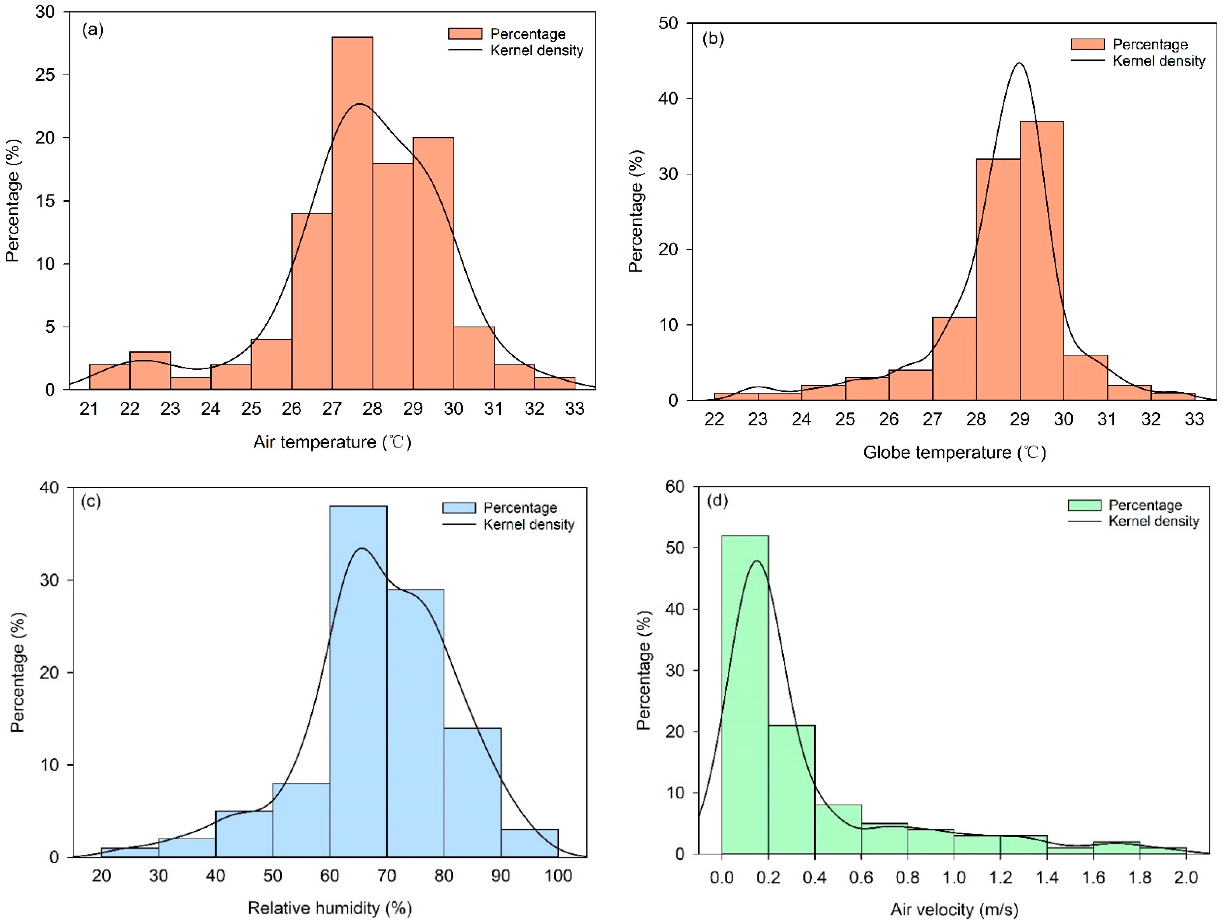
3.1. Objective Thermal Environment

3.1.1. Variation of Outdoor Thermal Environment

The results of the outdoor thermal environmental parameters during the field investigations are presented in

Table 6. The measured results of outdoor/indoor environmental parameters.

Variables	Unit	Height	1 Max.	2 Min.	Mean	3 SD
Outdoor air temperature (Ta-out)	°C	1.2 m	38.2	26.8	36.2	3.4
Outdoor relative humidity (RHout)	%	1.2 m	56.8	16.5	36.6	5.1
Outdoor air velocity (Va-out)	m/s	1.2 m	3.6	0.08	0.68	0.65
Solar radiation (SR)	W/m2	-	262.2	2.4	142.8	185.6
Indoor air temperature (Ta-in)	°C	0.6 m	31.2	21.6	27.7	1.7
		1.7 m	31.5	21.4	28.2	1.6
		3.3 m	32.8	22.1	28.5	1.3
Indoor relative humidity (RHin)	%	0.6 m	86.5	24.5	62.8	11.1
		1.7 m	85.0	26.2	63.7	11.0
		3.3 m	90.2	27.5	63.6	10.5
Indoor air velocity (Va-in)	m/s	0.6 m	1.5	0	0.16	0.21
		1.7 m	1.8	0.02	0.14	0.25
		3.3 m	2.0	0.02	0.22	0.18
Black globe temperature (Tg)	°C	0.6 m	32.6	22.8	29.1	1.6

Note: ¹ maximum value; ² minimum value; ³ standard deviation.

. It can be seen that the outdoor air temperature in Urumqi ranged from 26.8 °C to 38.2 °C, with mean and standard deviation (SD) values of 36.2 °C and 3.4 °C, respectively. Outdoor relative humidity oscillated between 16.5% and 56.8% and was less than 40% most of the time (mean = 36.6%, SD = 5.1%). Except for the outdoor instantaneous air speed values of a specific period being large (≥3 m/s), the mean and SD values were 0.68 m/s, 0.65 m/s, respectively.

3.1.2. Variation of Indoor Thermal Environment

Table 6 summarized the different values of the measured indoor environmental parameters. Comparing with Figure 4a, the variations in indoor air temperatures were mainly distributed from 26 °C to 30 °C and the maximum value even exceeded 32.5 °C. As the height increased, the temperatures rose slightly. Around 75% of the values were higher than 27 °C, which surpassed the neutral (comfort) temperatures in other previous studies. The globe temperature, shown in Figure 4b, was slightly higher than air temperature due to the coupling effect of radiation and convection being considered. The highest frequency varied from 27 °C to 31 °C with the average and SD values of 29.1 °C and 1.6 °C, respectively. Figure 4c showed the variation of indoor relative humidity in summer, as the ECS reduced the air temperature by absorbing heat through evaporation and the process carried large amounts of moisture into the ambient air, the mean values of RH located at a higher level (approximately 60–90%) than NV [44], AC [19], and MM [24] buildings. Figure 4d presented the variation of indoor air velocity in summer, the values were basically between 0.14 m/s and 0.23 m/s, over roughly 50% of which were below 0.2 m/s. The primary reason was ease of affectation by the outdoor environment and always being maintained in a steady state, which generally satisfied the reference in the ASHRAE Standard [9].

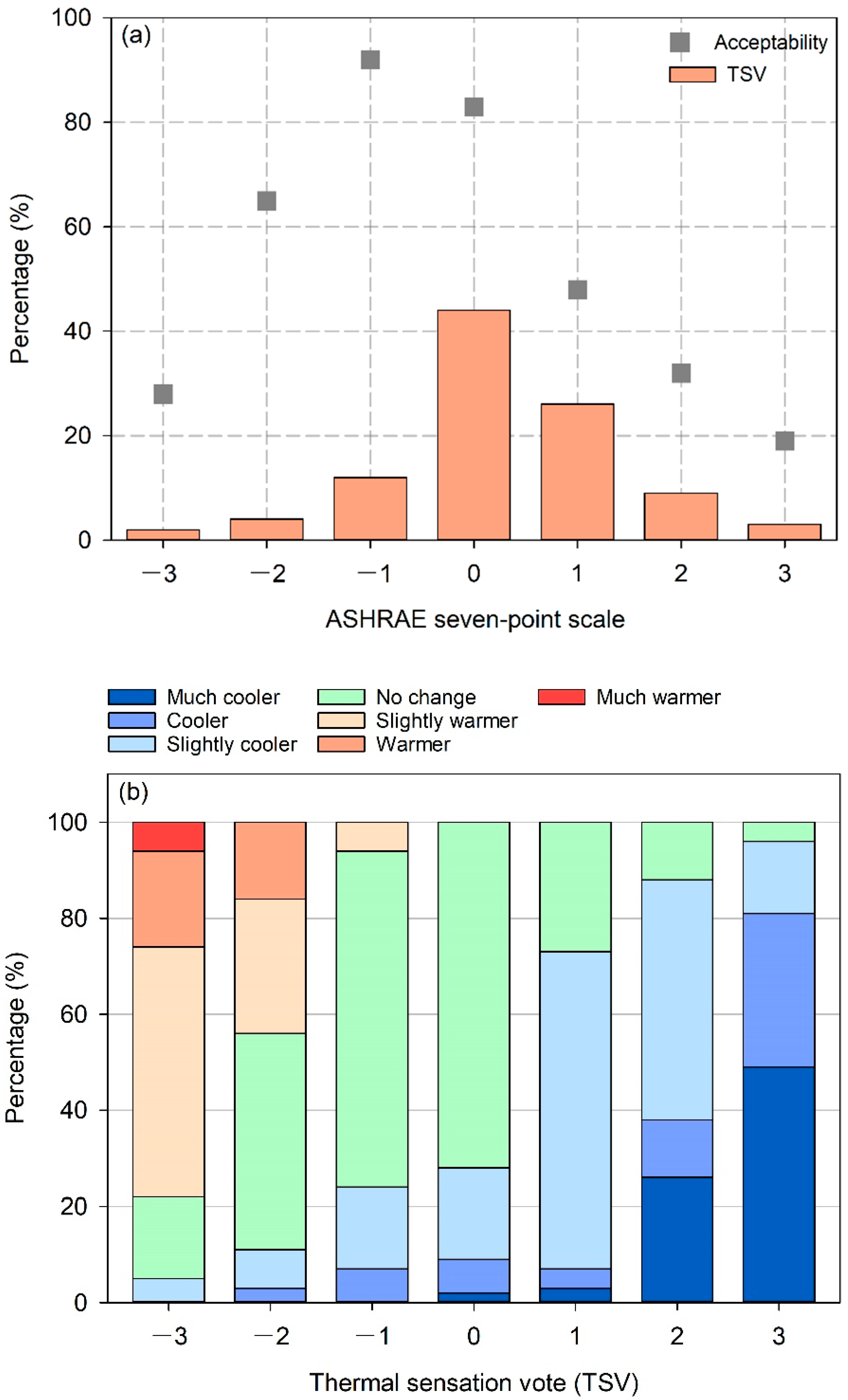
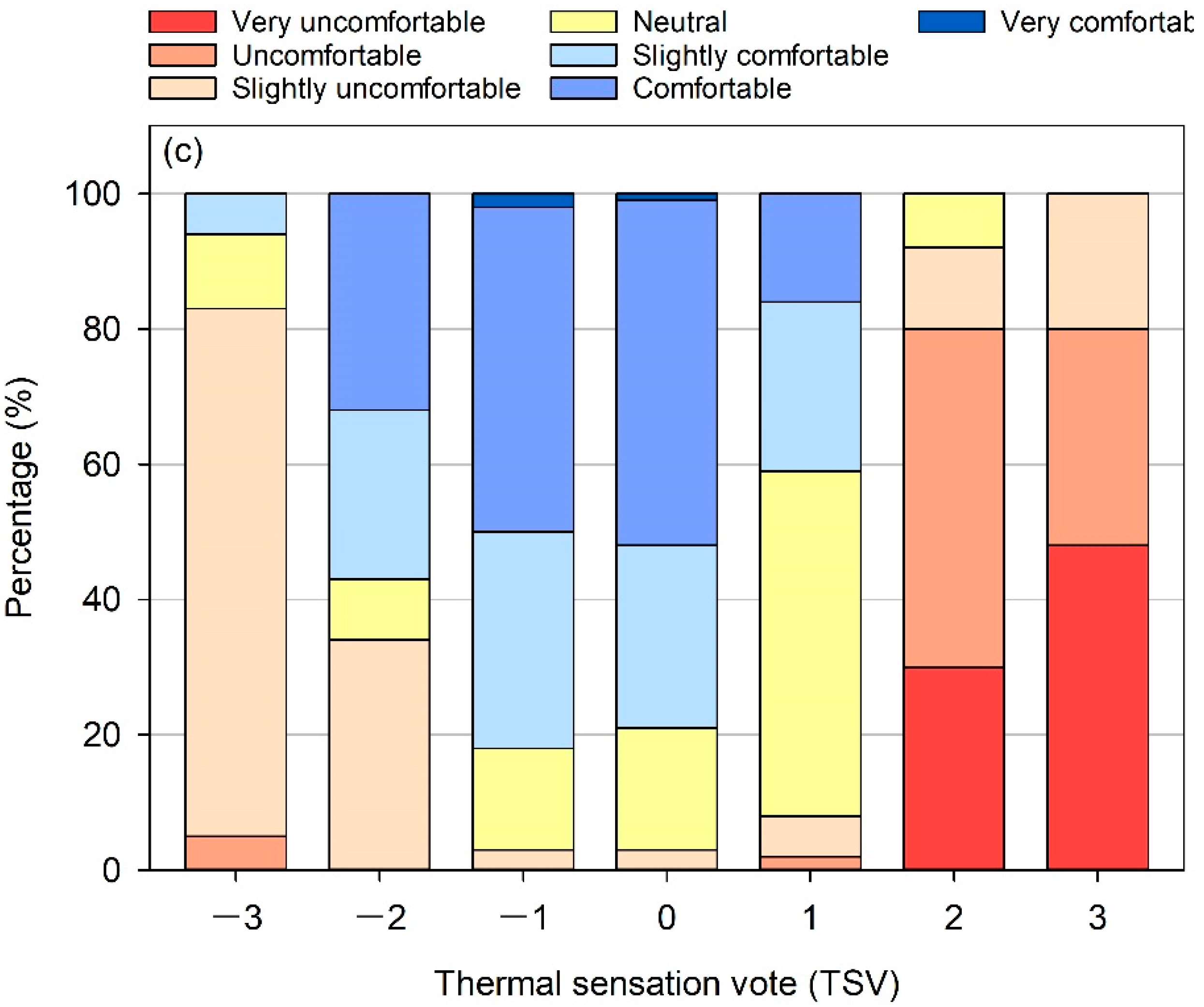
3.2. Subjective Thermal Responses

Figure 5a shows the results of the thermal sensation vote (TSV) and overall thermal acceptability vote (TAV) in each TSV interval. The highest percentage of votes were neutrality (TSV = 0), in which approximately 44% and beyond 80% of the occupants’ TSV were distributed across the comfort bandwidth (±1). The proportions of thermal acceptability all surpassed 80% when TSV scale was “slightly cool” (−1) and “neutral” (0), and less than 50% on the warmer side (1 to 3). It illustrated that subjects were more inclined to cooler indoor environments than to warmer ones in summer. In terms of the thermal expectation vote (TEV), Figure 5b summarized the proportion of ingredients for the TEV in each TSV scale. The percentage of cooler preference (the sum of “slightly cooler”, “cooler”, and “much cooler”) maintained an upward trend with the level of TSV increasing from −3 to 3, while the warmer appeals gradually declined. The highest votes of “no change” occurred when the TSV equaled 0 that was approximately 72%, and still 28% of the occupants preferred a cooler environment on this scale. The outcomes indicated that the neutral state (TSV = 0) was not always the best strategy for all participants; the variation between thermal sensation and expectation may have existed to some extent, which also confirmed the basic conclusion of previous studies by Z. Wu [26], R. Thapa [45], S.A. Damiati [46], and M.K. Singh [47]. Based on the coupling effect of indoor air temperature, relative humidity, and wind speed, the overall thermal comfort vote is presented in Figure 5c. Neutrality and comfort state (including “slightly comfortable”, “comfortable” and “very comfortable”) all exceeded 90% between −1 and 1. Although a significant proportion of subjects expected a cooler environment when TSV equaled 1, there were still around 51% and 41% of the people feeling neutral and comfortable, further revealing that the perennial living conditions had improved the heating resistance of local residents in summer.

3.3. Neutral (Comfort) Temperature

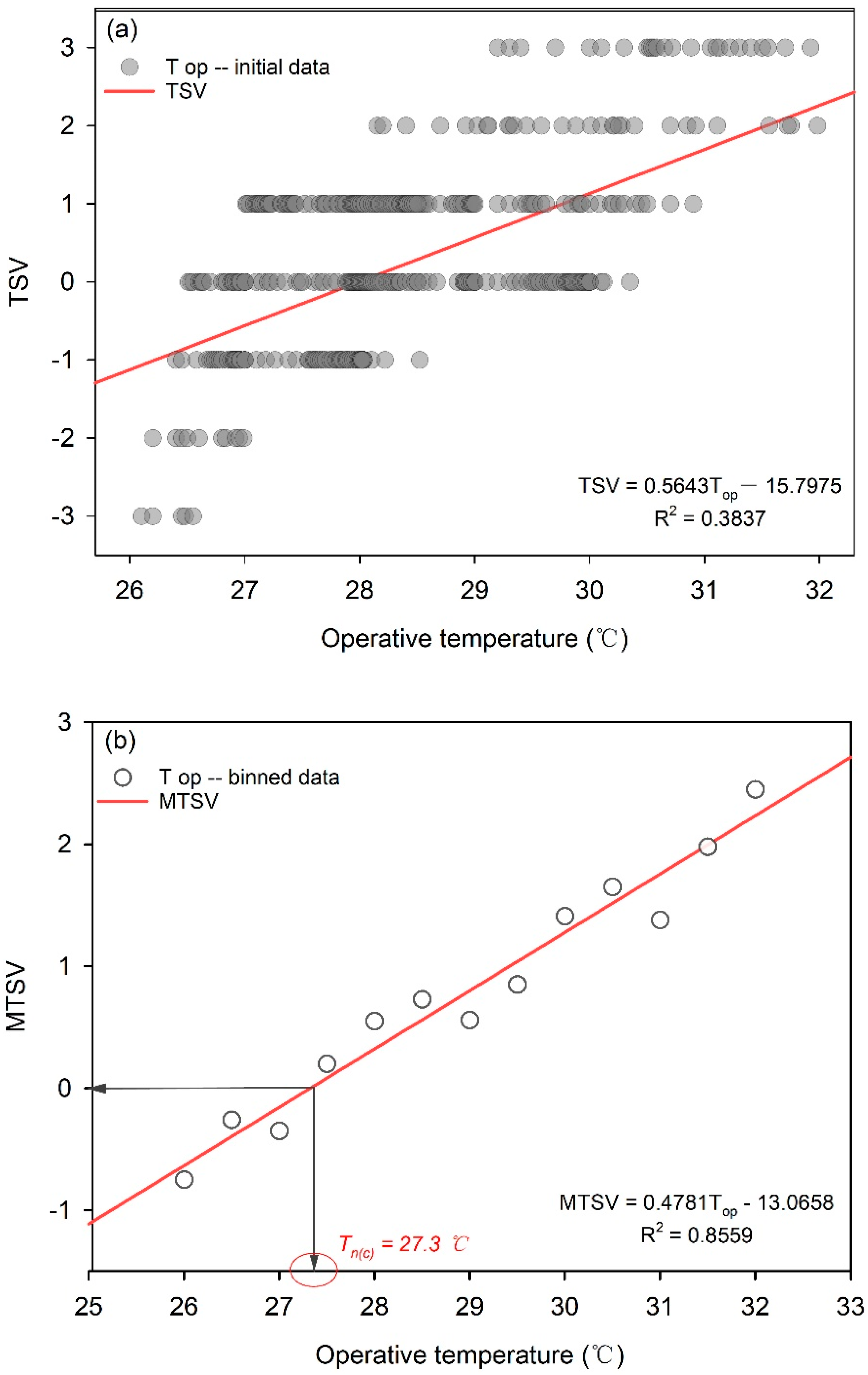
3.3.1. Linear Regression Analysis

The exploration of the critical point at which occupants felt neither too cold nor too hot, neutral temperature, also known as comfort temperature, was carried out using linear regression analysis between indoor operative temperature (T_op) and thermal sensation vote (TSV). T_c is determined when TSV equals zero. The initial data for TSV and T_op is collected in Figure 6a, from which the regression equation is shown as Equation (6). The slope of the fitted curve was 0.5643, which illustrates that approximately 1.78 °C modification in T_op led to one unit change in TSV.

TSV = 0.5643T_op − 15.7975 (R² = 0.3837, p < 0.05)

(6)

Furthermore, considering the diversity of factors that affect thermal sensation and the differences among individuals, numerous researchers have adopted the mean thermal sensation vote (MTSV) instead of the TSV [18,21,27,28]. In the current research, by setting the binned data at a 0.5 °C interval of T_op to receive the linear regression model between T_op(mean) and MTSV in Figure 6b, it can be seen that MTSV is well fitted with T_op by the specific linear equation shown in Equation (7).

MTSV = 0.4781T_op − 13.0658 (R² = 0.8559, p < 0.05)

(7)

It is obvious that, when comparing the neutral temperature obtained by direct regression analysis (T_c = 27.9 °C), the outcomes calculated by bin method (T_c = 27.3 °C) were basically in agreement. Although the determination coefficient (R²) increased significantly, it was also consistent with the model assumptions made by C. Fu [18] and regarded as a reasonable value. Furthermore, it is slightly higher than the results of AC, NV, and MM mode in Table 1 due to the specific local climate and psychosomatic adaptation.

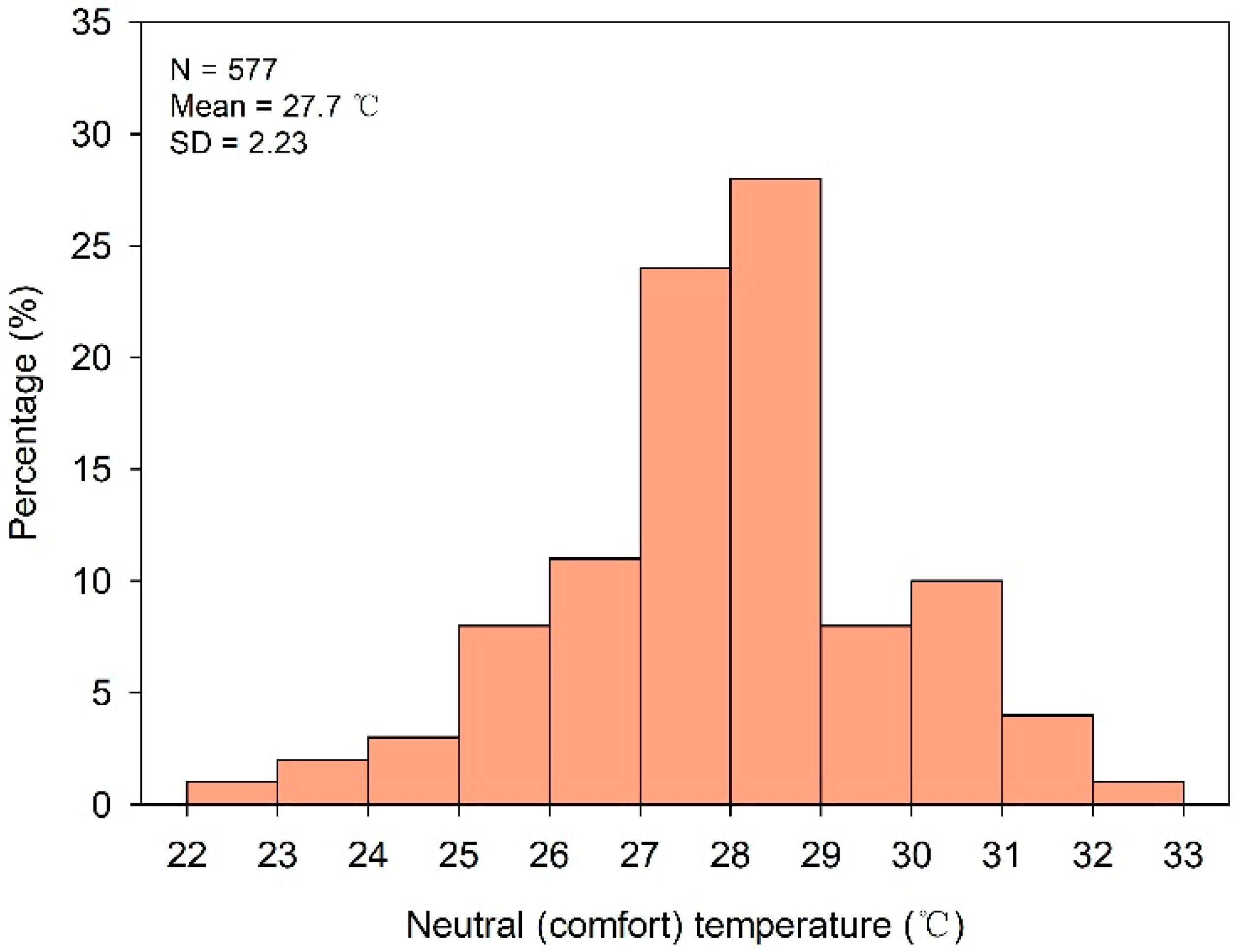
3.3.2. Griffiths Constant Method

On account of the limitations of experimental conditions, this research applied the Griffiths constant method to further calculate the indoor comfort temperature in summer and avoid the errors caused by relatively small sample size. It recommends adopting a simple standard value as a linear regression coefficient (Griffiths constant) between the thermal sensation vote and operative temperature. Three empirical values (0.25, 0.33, and 0.50) were probed in previous studies by P. Tewari [16], Z. Wu [26], M.A. Humphreys [48], and H.B. Rijal [49]. In the current study, a value of 0.50 was adopted for further calculation mainly because there was almost no difference between the mean globe temperature (TSV = 0) and comfort temperature. Figure 7 summarized the distribution of indoor comfort temperature with the binned data at 1 °C. The comfort temperature interval ranged from 22 °C to 33 °C and above 80% of the values were scattered between 26 °C and 30 °C. In addition, the mean value of the comfort temperature was 27.7 °C, which is basically similar to the results calculated by linear regression (27.3 °C).

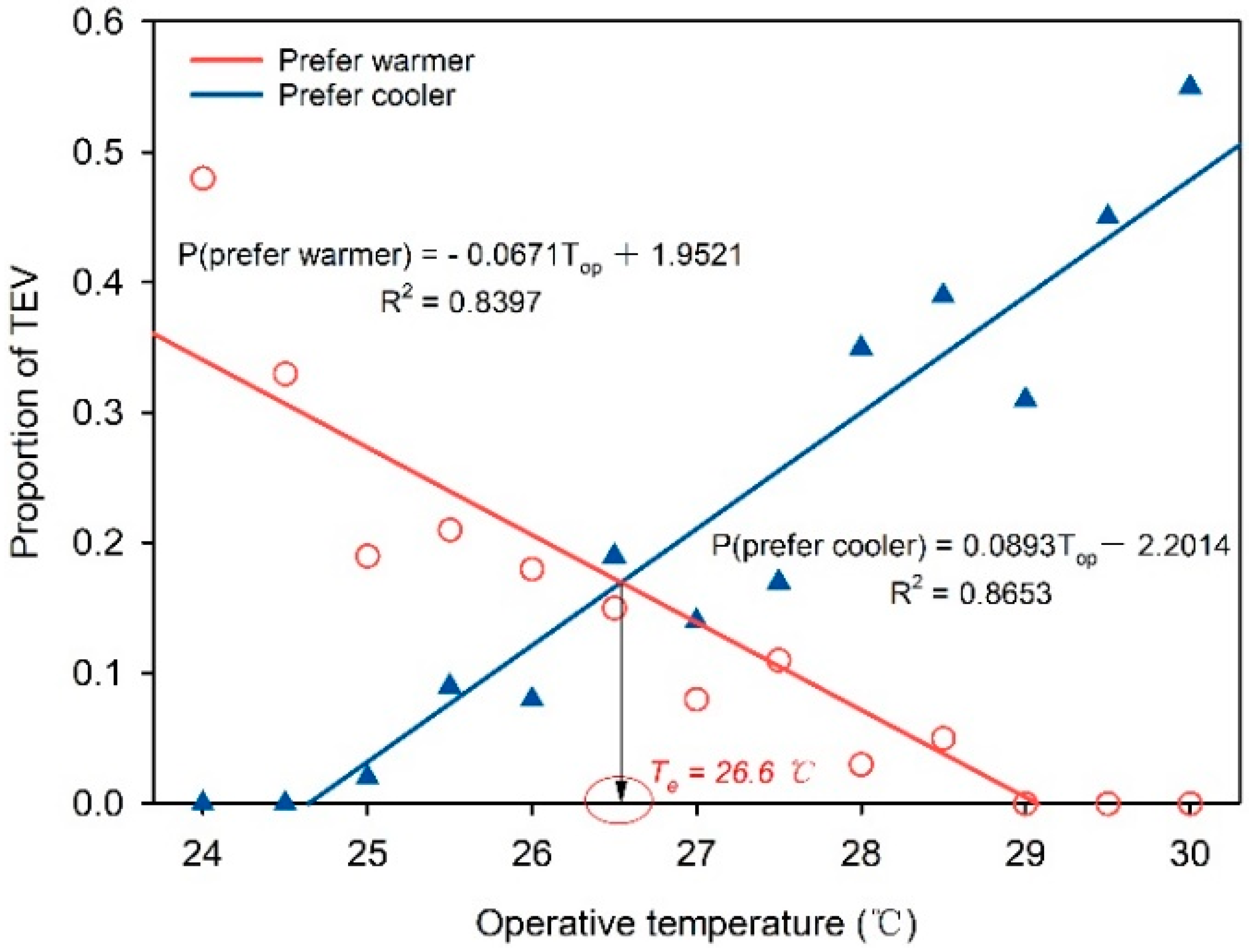
3.4. Expectative Temperature

According to the discussion in Section 3.2, there might be a disparity between neutral temperature and expectative temperature. In other words, occupants generally preferred a warmer state over the neutral one in a cold climate, and pursued cooler conditions in hot climates, which also had been confirmed in former studies [24,26,50]. In this section, a binned method combined with a half-degree-Celsius and weighted linear regression analysis were adopted to evaluate the indoor expectative temperature. All of the thermal responses were divided into two groups: namely “prefer warmer” (TEV > 0 + half votes of “no change”) and “prefer cooler” (TEV < 0 + half votes of “no change”). In addition, we calculated the percentage of votes in “prefer warmer” and “prefer cooler” for each 0.5 °C interval, respectively. Then regressing against with the corresponding operative temperature to obtain two regression models. Figure 8 presents the results of expectative temperature for investigated ECS office buildings, and the regression equations are listed as follows in Equations (8) and (9).

P (prefer warmer) = −0.0671T_op + 1.9521 (R² = 0.8397, p < 0.001)

(8)

P (prefer cooler) = 0.0893T_op − 2.2014 (R² = 0.8653, p < 0.001)

(9)

Based on Figure 8, the value of indoor expectative temperature (T_e) appeared at the intersection point of two fitting equations, which was 26.6 °C in this study. It was lower by approximately 0.7 °C than neutral (comfort) temperature (27.3 °C by linear regression). The deviation between T_e and T_c was smaller than in previous studies by C. Fu [18] (1–3 °C) and J.M.Y. Tse [24] (0.4–1.9 °C), which was mainly due to the occupants’ higher physiological adaptation to the local dry hot climate in summer.

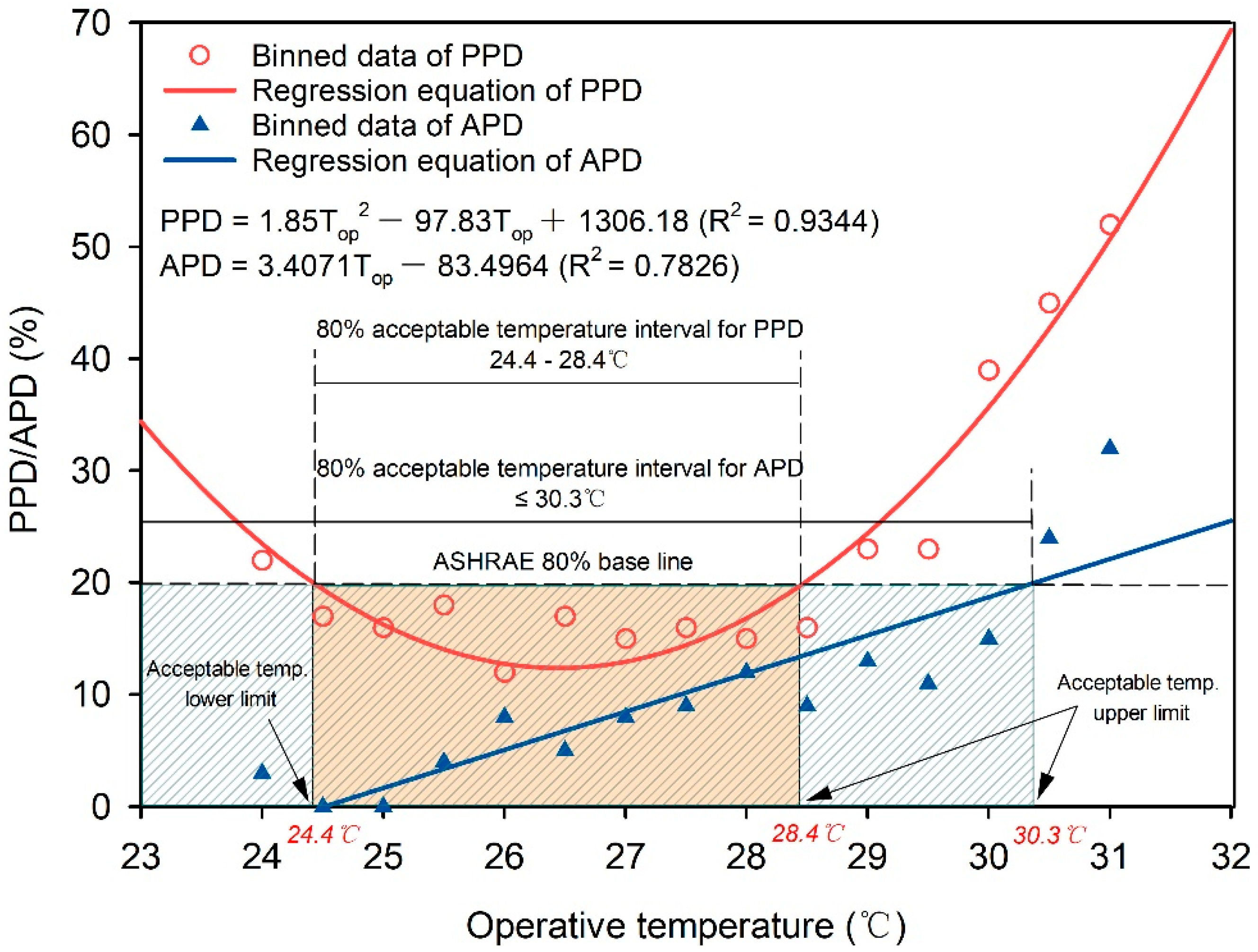
3.5. Acceptable Temperature Interval

In the quest to explore the value limitations of the acceptable temperature range, typical questions were set in the questionnaire for occupants, such as “Could you accept the thermal environment at the moment?” Meanwhile, the occupants’ percentage of acceptance rates within each temperature interval were calculated, and then a multiple regression method was adopted to determine the relationships between acceptance rate and operative temperature. As discussed above, the TSV was not in the neutral state when the actual percentage of dissatisfaction (APD) was lowest. Instead, it was asymmetrically distributed on both sides of TSV = 0. Therefore, the APD and PPD were calculated with 0.5 °C binned data against the indoor operative temperature in Figure 9. The regression models were presented as Equations (10) and (11).

PPD = 1.85 T_op² − 97.83T_op + 1306.18 (R² = 0.9344, p < 0.001)

(10)

APD = 3.4071T_op − 83.4964 (R² = 0.7826, p < 0.001)

(11)

According to ASHRAE-55 [9], an acceptability limitation of 80% was defined as the evaluation criteria for receiving the indoor acceptable temperature interval; see Figure 8. The predicted limitation of the 80% acceptable interval was 24.4–28.4 °C, while the upper limit of the actual situation was 30.3 °C, 1.9 °C higher than that calculated by PPD. The wider bandwidth of temperature acceptability illustrated that the local occupants with higher environmental adaptation and the conventional PMV-PPD model underestimated the subjects’ heating tolerance in ECS office buildings.

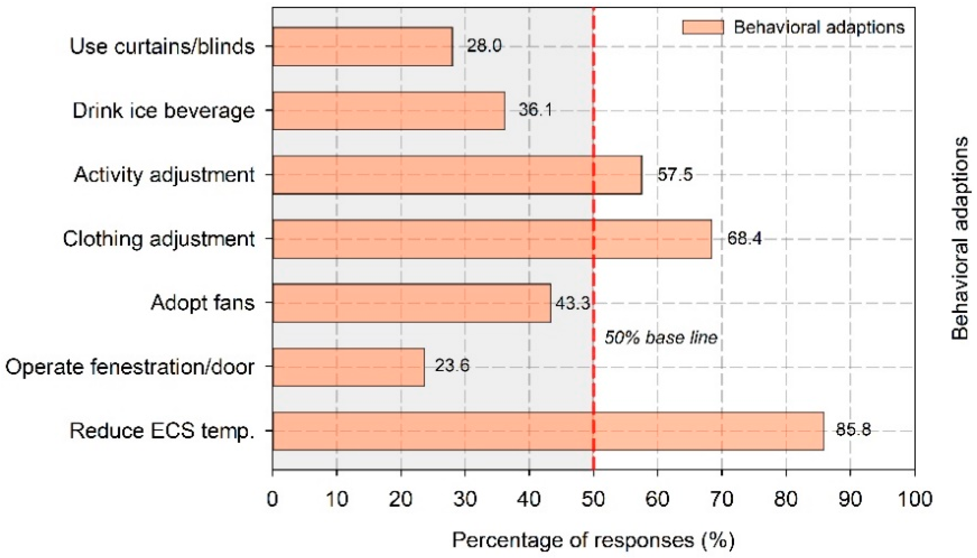
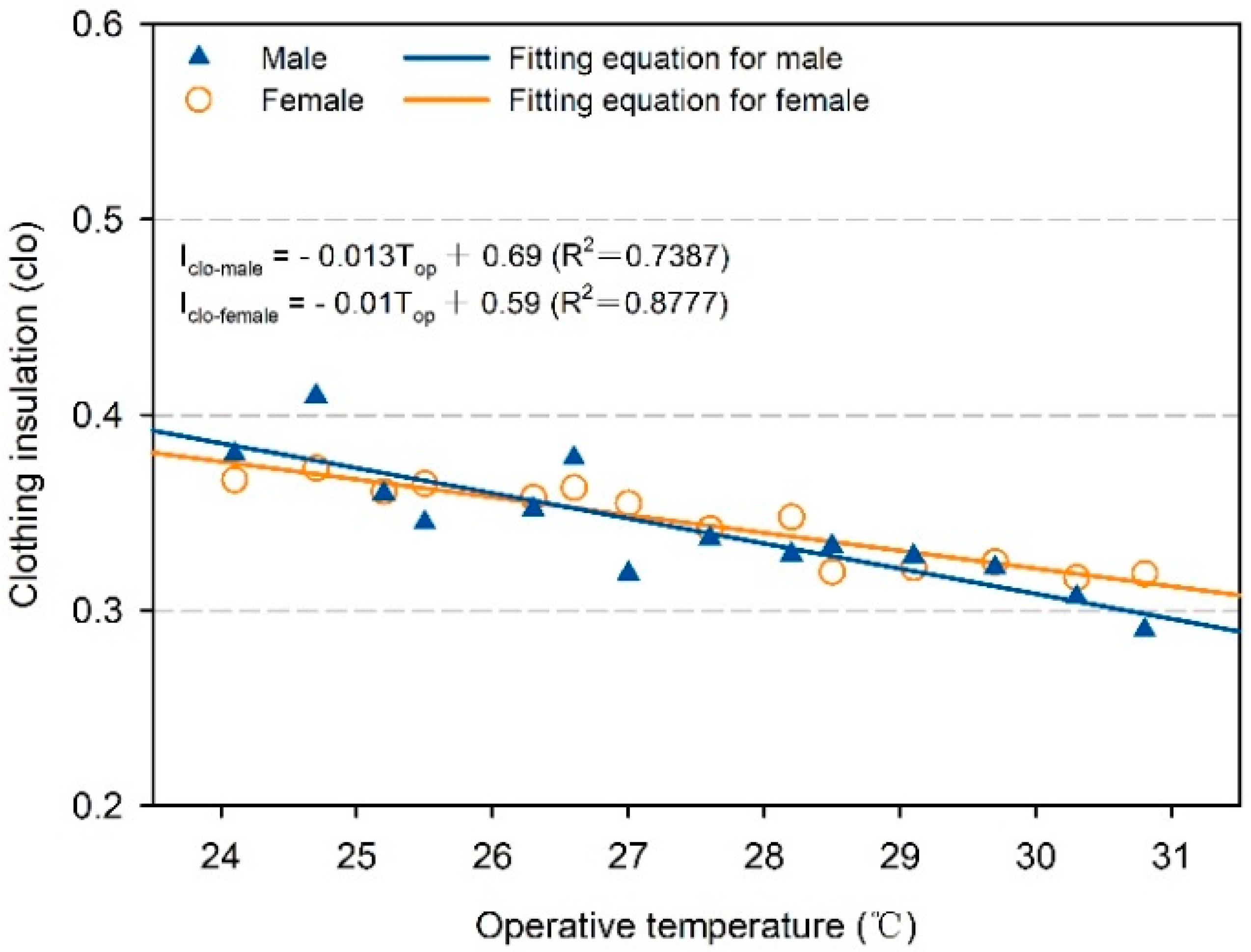
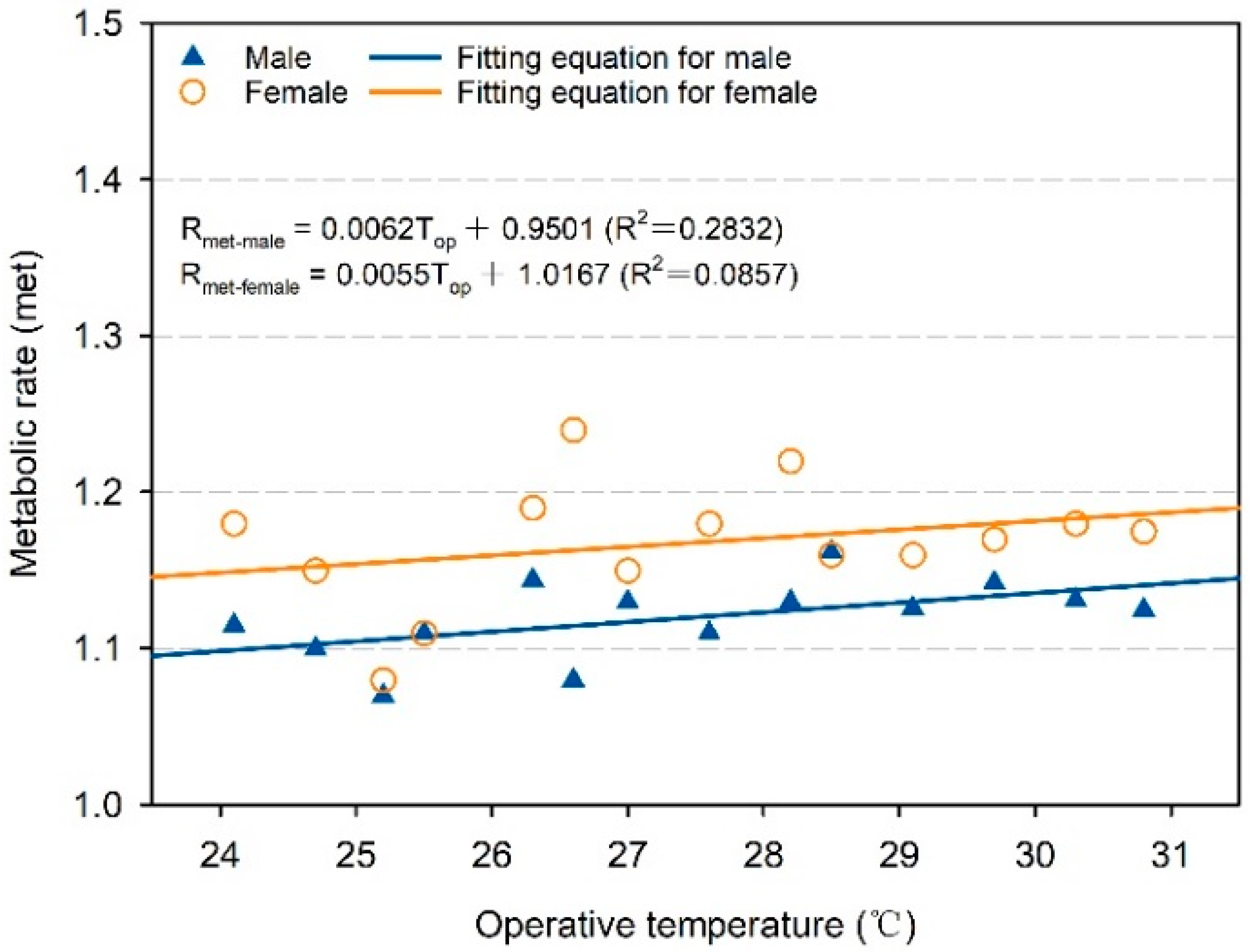
3.6. Thermal Adaption

Thanks to the conventional predicted model (PMV-PPD) being unable to reflect the objective situation accurately, it is meaningful to further analyze the quantitative relationships of body thermal adaptability. Generally speaking, adaptive regulation of human body mainly involves three aspects: behavioral, psychological, and physiological adaption [40,51]. Although the behavioral adaptions could be easily obtained via questionnaire survey, psychological and physiological adjustment need to be judged by a long-term process and past experience. Therefore, this section focused on the relationships between three adaptive mechanisms mentioned above and indoor/outdoor temperatures. Section 3.6.1 discusses behavioral adaption, and adaptive comfort models that consider the coupling relationship between psychological and physiological adaption were applied are discussed in in Section 3.6.2.

3.6.1. Physical and Auto-Adaptive Behavior

Behavioral adaptions including actions taken intentionally or unintentionally to change one’s thermal equilibrium, which can be divided into physical adjustment (using curtains/blinds, switching on/off ECS, etc.) and auto-adaptive actions (such as changing clothing, changing activity levels, etc.). Figure 10 summarized the intent frequency of seven common modes of behavioral regulations when subjects felt hot in summer with evaporative cooling systems. The top three choices that surpassed the base line of 50% were reducing the set point of ECS temperature, changing clothing and decreasing activity levels, with the consequence approximately at 85.8%, 68.4%, and 57.5%, respectively. Although the use of equipment could satisfy the compensation requirements of thermal comfort, a large amount of energy would be wasted by operating windows/doors at irregular times.

During the survey period, we observed the actual clothing situation of local subjects in 8 office buildings. From which two of the most common clothing combinations could be summarized: (a) thin trousers, short-sleeve shirt, and sneakers; (b) walking shorts, T-shirt, and sandals. Meanwhile, based on the recommended value of clothing insulation in ASHRAE-55 [9], the total values were approximately 0.34 clo (type “a”) and 0.30 clo (type “b”), respectively. Furthermore, with the grouping of the indoor operative temperature by 0.5 °C, the mean T_op and the corresponding average clothing insulation of each group were calculated in Figure 11. It can be easily seen that a negative correlation existed between T_op and clothing insulation regardless of gender, but the slope was slightly different. A 1 °C increase in T_op could lead to 0.013 clo and 0.010 clo decreases in clothing insulation for males and females, respectively. The tiny deviation reflected the men with slightly greater dependence on clothing than women in this region.

Due to the ability of thermal discomfort to be effectively regulated by changing activity levels, the relationship between T_op and the metabolic rate was also probed with the same method, as shown in Figure 12. The subjects mostly maintained the sitting position with light physical activity during the period of investigation. Based on ASHRAE-55 [9], the metabolic rate was defined as M ≤ 1.2 met (70 W/m²). From the results of the weighted linear regression, there was no obvious linear relationship between T_op and metabolic rate as the determining coefficient (R²) of the fitting equation was 0.2832 and 0.0857 for males and females, respectively. This further manifested that metabolic rate is more influenced by various activity levels than surrounding environmental parameters.

3.6.2. Physical and Auto-Adaptive Behavior

Using an adaptive approach that emphasizes the importance of long-term life experiences in thermal sensation and environmental parameters, R.J. de Dear [15] and J.F. Nicol [52] explored the relationships between prevailing mean outdoor temperature (T_pma) and comfort temperature. They confirmed that the T_pma is a more accurate index than that of outdoor instantaneous climatic values. Therefore, in current study, the adaptive model for occupants in ECS office buildings was established by adopting regression analysis among T_c (mainly refer to −1 ≤ TSV ≤ 1) and T_pma (average temperature at the matching time with each T_c, which ranged from 26.8 °C to 38.2 °C according to the algorithm of Equation (1)). Figure 13 showed the relationships between indoor operative temperatures (comfort scatters) and prevailing mean outdoor temperature, with the linear fitting formula presented in Equation (12).

T_c = 0.06T_pma + 26.17 (R² = 0.3686, p < 0.001)

(12)

In accordance with the theory of thermal acceptability, there were 80% and 90% acceptable rate limits corresponding to the PMV of ±0.85 and ±0.5 [13,53]. The four indicators were applied to explore the regression model via Equations (7) and (12). Additionally, from Figure 13, the equations of the lower and upper limits of 80% and 90% acceptable indoor comfort temperatures were obtained; see Equations (13)–(16).

T_80%,UL = 0.06T_pma + 27.95

(13)

T_{80%, LL} = 0.06T_pma + 24.39

(14)

T_90%,UL = 0.06T_pma + 27.21

(15)

T_{90%, LL} = 0.06T_pma + 25.13

(16)

From the calculation results, two indoor acceptable operative temperature intervals (referring to 80% and 90%) were received by approximately 1.78 °C (interval/2, i.e., 3.56 °C/2) and 1.04 °C (interval/2, i.e., 2.08 °C/2), respectively. As the prevailing average outdoor temperature increased, comfort temperatures were also added slightly and mainly distributed from 27.1 °C to 28.9 °C for the 90% limit area. Meanwhile, the slope of lower/upper limit equations were basically consistent with the adaptive model. Although regional differences (climate, culture, physiological characteristics, etc.) may lead to adaptive models varying from other studies, it provided a comparative reference for the definition of comfort zones under the current norms of ASHRAE-55 [9].

4. Discussion

4.1. Comparison with Predicted Thermal Sensation

As mentioned above, the “comfort zone method” proposed in ASHRAE-55 was according to the algorithm of the PMV model [9], which defined a typical indoor thermal environment with 80% acceptability (based on 10% overall and 10% partial thermal comfort dissatisfaction). In the current research, the indoor air velocity was distributed between 0.14 m/s and 0.23 m/s for most of the time, with an average value of approximately 0.17 m/s, lower than the upper limit specified in ASHRAE-55 (still air of 0.2 m/s). In addition, the mean value of physical activity 1.1 met with a clothing insulation of 0.36 clo also conformed with the basic requirement of that standard (1–1.3 met, less than 0.5 clo, respectively) [9]. Therefore, the data on indoor operative temperatures with specific humidity ratios in ECS office buildings were recorded to compare with the thermal comfort zone of ASHRAE-55, for questing the relationships between the adaptive model and PMV algorithm.

In Figure 14, the indoor air state parameters were determined by operative temperature (X-axis) and relative humidity with a certain amount of moisture content (Y-axis). There were scarcely any comfort dots distributed within the recommended comfort zone (light orange shaded area), most of which were scattered across the upper limit of ASHRAE-55; the wider acceptable temperature interval with higher relative humidity in ECS office buildings was beyond the recommended zone. It suggests that the PMV model adopted in ASHRAE-55 cannot be an appropriate method for assessing this working mode in Urumqi. The causes of the deviation are mainly due to three aspects as follows: Firstly, thermal comfort (coupling effect) and thermal neutrality (TSV = 0) were regarded as the same concept during the process of establishing the PMV model. However, the former described a coupling effect of behavioral, psychological, and physiological sensations, which was difficult to adopt a certain fixed parameter for judging the comfort evaluation for. In other words, the PMV model based on thermal neutrality may to some extent impose inevitable limitations on the predicted results. In addition, the heat dissipation of evaporation in the heat balance equation using PMV takes the comprehensive influence of four indexes into account, namely heat loss by skin vapor diffusion (E_sv), heat loss by sweat diffusion (E_sd), heat loss by latent respiration (E_lr) and heat loss by dry respiration (E_dr) [13]. Nevertheless, the calculations of mean skin surface temperature (T_sk) and sweat evaporation were both made under the assumption that within the range of the thermal neutral state, T_sk and E_sd were fixed values because they were only affected by the metabolic rate. Thus, the PMV equation could accurately reflect the offset of thermal comfort when occupants felt uncomfortable at some special period, such as during the process of sweating profusely. Lastly, although it gave full consideration to the six major factors affecting thermal comfort, the uniqueness of the subjects did not cover the degree of climatic adaptation and self-regulation for local occupants in different regions.

In order to narrow the deviation between actual sensation votes (TSV) and predicted voting results (PMV), researchers have made unremitting efforts for several generations. P.O. Fanger [54] pointed out that the gap is mainly due to the neglect of occupants’ expectations and psychological adaptation to the actual environment. An expectation factor named “e” was later carried out to modify the original PMV model, with the specific mathematical model described as Equation (17) [54]:

ePMV = e × PMV

(17)

where the two essential conditions of the expectation factor (e, 0.5–1) were duration time period of the hot weather and the comparison between local air-conditioned and non-air-conditioned buildings. In Urumqi, the weather is hot during summer season and in a certain amount of ECS office buildings, which belonging to the medium expectation level, the value of 0.8 for “e” was adopted for further analysis.

Based on the better-fitting relationship between T_c and T_pma, R. Yao [55] defined the principle of the “black box” in automatic control theory and proposed an adaptive coefficient “λ” that reflects the influence of thermal sensation to correct the raw equation. Meanwhile, the adaptive predicted model (APMV) was obtained by adopting the least square method as shown in Equation (18).

APMV = PMV/(1 + λPMV)

(18)

where the adaptive coefficient (λ) for cool and warm conditions were both taken the society, culture, climate, psychology, and behavioral adaptation into account seriously. According to the recommended values of the Chinese National Norm [56], λ for public buildings in Urumqi (severe cold zone C) is equal to −0.5 for cool conditions (PMV < 0) and 0.24 for warm conditions (PMV > 0).

As discussed above, the comparison of results between TSV (actual mean vote in Figure 5b from questionnaires), PMV (predicted index), ePMV, and APMV (predicted adaptive index) is presented in Figure 15. By contrasting the TSV with PMV, a relatively large error existed compared to ePMV and APMV, which illustrated that the original model underestimated the occupants’ heat tolerance in summer. The higher indoor operative temperature, the larger the deviation. Additionally the phenomenon of the “scissors difference” was also attested by J. Jiang [31] and Z. Zhang [57]. To further explore the adjustment results, we set the two values as the interval limitation. Point 1 is the intersection of ePMV (green solid line) and APMV (red solid line), which corresponds to the X-coordinate of approximately 27.6 °C. Point 2 is determined by the absolute value of the Y-coordinate difference between TSV and ePMV/APMV. With the intercepts as “a” (|YTSV–YePMV|) and “b” (|YTSV–YAPMV|), respectively, when “a” was equal to “b”, point 2 was obtained at around 29.8 °C in this research. In this way, three intervals were defined by those two points. When T_op was lower than 27.6 °C or higher than 29.8 °C, it could be observed that the fitting effects of ePMV were better than the APMV when comparing with authentic thermal sensation. The opposite situation appeared by T_op ranging from 27.6 °C to 29.8 °C, which showed a smaller error in the APMV. Much less considered but no less important, although the proposed adaptive predicted models could effectively narrow the gap in the actual situation, the accuracy was within a certain operative temperature range. Those results may vary from each other under different climatic conditions and indoor operating modes. In this study, more appropriate intervals for the usage of the adaptive predicted model of APMV and ePMV were gained at 27.6 °C < T_op < 29.8 °C, T_op < 27.6 °C/T_op > 29.8 °C, respectively.

4.2. Comparison with Previous Research using Different Modes

By using evaporative cooling systems in office buildings during the summer season, the indoor neutral temperature was around 27.3 °C, 0.7 °C higher than the expectative temperature (26.6 °C). The comfort interval for the 90% and 80% acceptable levels were about 27.1–28.9 °C, 26.4–30.3 °C, respectively. Although a certain percentage of occupants (exceeding 40%) could accept the current environment, there was still a willingness among them to be slightly cooler. Furthermore, the overall acceptability in TSV = −1 was also higher than in the neutral state (compared with Figure 5a,b). It was in agreement with the basic conclusion by P. Tewari [16] and Z. Zhang [57].

In addition, to better understand the differentiation characteristics of ECS buildings, we also performed a regression analysis on environmental parameters without ECS (NV mode) in the same testing period.

Table 7. Comparison of adaptive model with previous research using different modes.

Mode	Scholars	Location	Season	Type	Adaptive Model
1 ECS	Tewari [16]	Jaipur	Summer	Office	5 Tc = 0.22 6 Trm-out + 21.5
	Current research	Urumqi	Summer	Office	Tc = 0.06Tpma-out + 26.17
2 AC	Indraganti [62]	Qatar	All	Office	Tc = 0.049Trm-out + 22.5
	Fu [18]	Guangzhou	Summer	Office	Tc = 0.18 7 Tpma-out + 22.89
	López-Pérez [63]	Tuxtla Gutiérrez	Summer	Classroom	Tc = 0.13Trm-out + 22.7
	Ricciardi [64]	Northern Italy	Summer	Office	Tc = 0.15Trm-out + 19.35
	Rijal [65]	Tokyo/Yokohama	All	Office	Tc = 0.065Trm-out + 23.9
3 NV	Current research	Urumqi	Summer	Office	Tc = 0.17Tpma-out + 23.94
	Yu [22]	Shanghai	Summer Winter	Dwelling	Tc = 0.418Tpma-out + 15.96 Tc = 0.706Tpma-out + 9.375
	Indraganti [58]	Hyderabad	Summer	Office	Tc = 0.26Trm-out + 21.4
	Dhaka [59]	Jaipur	Summer Winter	Office	Tc = 0.75To + 5.4
	Singh [60]	India	Autumn	Office	Tc = 0.36To + 16.94
	Fu [18]	Guangzhou	Winter	Office	Tc = 0.78Tpma-out + 9.42
	López-Pérez [63]	Tuxtla Gutiérrez	Summer	Classroom	Tc = 0.32Trm-out + 18.45
	Thapa [61]	Mirik	All	Office	Tc = 0.64Tpma-out + 9.02
	Rijal [65]	Tokyo/Yokohama	All	Office	Tc = 0.21Trm-out + 20.8
4 MM	Rupp [66]	Florianópolis	All	Office	Tc, NV = 0.56Tpma-out + 12.74 Tc, AC = 0.09Tpma-out + 22.32
	Martin [27]	Seville	All	Office	Tc = 0.2427Trm-out + 19.284

Note: ¹ evaporative cooling system; ² air-conditioned buildings; ³ naturally ventilated buildings; ⁴ mixed mode buildings; ⁵ indoor comfort temperature; ⁶ running mean outdoor temperature; ⁷ prevailing mean outdoor temperature.

summarized the comparison results of current research with previous thermal adaptive models using different modes. The results observed that the actual T_c in ECS buildings were higher than AC and MM mode, and lower than NV mode. The reasons mainly, attributed to usage behaviors and thermal history, varied from each other across different modes. For AC mode, the indoor environment was less influenced by outdoor temperature owing to windows and doors being closed for most of the time; a relatively stable environment may reduce occupants’ thermal sensitivity to surrounding physical stimuli. Additionally, the more flexible operating modes in ECS buildings made their cooling effect slightly less than that of AC, which lead to the higher heating tolerance of occupants in summer. For the NV mode, the phenomenon that dominated the surrounding environment was even more pronounced, and the resulting upper limit of acceptable temperature was higher than in this study by about 0.85–2 °C in [18,22,58,59,60,61]. Therefore, the significant differences above indicate that it is necessary to establish an adaptive model for ECS buildings instead of depending on results provided by AC and NV modes.

4.3. Potential Application of Adaptive Model

There is no doubt that an adaptive model can better predict the neutral temperature of occupants by using outdoor climate data. Yet, how it could be potentially applied in other regions? As a matter of fact, it depends on two prerequisites: (1) cooling degree days (CDDs) of ECS; (2) potential of regional evaporation. Only considered climatic conditions and ignored CDDs would lead the areas with high evaporation potential and fewer CDDs would require classification in high application zones, further resulting in the waste of investment and deviations in occupants’ thermal history. Through a trade-off analysis of the two factors above, the adaptive model of ECS buildings in Urumqi may be potentially applied in the northeastern Xinjiang autonomous region, northwest Gansu province, and western Inner Mongolia autonomous regions. For one thing, the difference between dry and wet bulb air temperatures in these regions are approximately 12.1~16.8 °C, where the atmosphere is rich in dry air energy. For another, this kind of climate zone has a large requirement for ECS in summer and with similar CDD values. As for worldwide, the adaptive model may also have reference value for optimizing indoor design parameters during the cooling season in Turkey, Kazakhstan, Iran, and other “Belt and Road” (B&R) developing countries.

5. Conclusions

With the conjoined analyses above, this research conducted a systematic investigation on office buildings with evaporative cooling systems (ECS) during the summer season in Urumqi, China. According to the results of the data calculation, the following conclusions can be summarized:

(1)

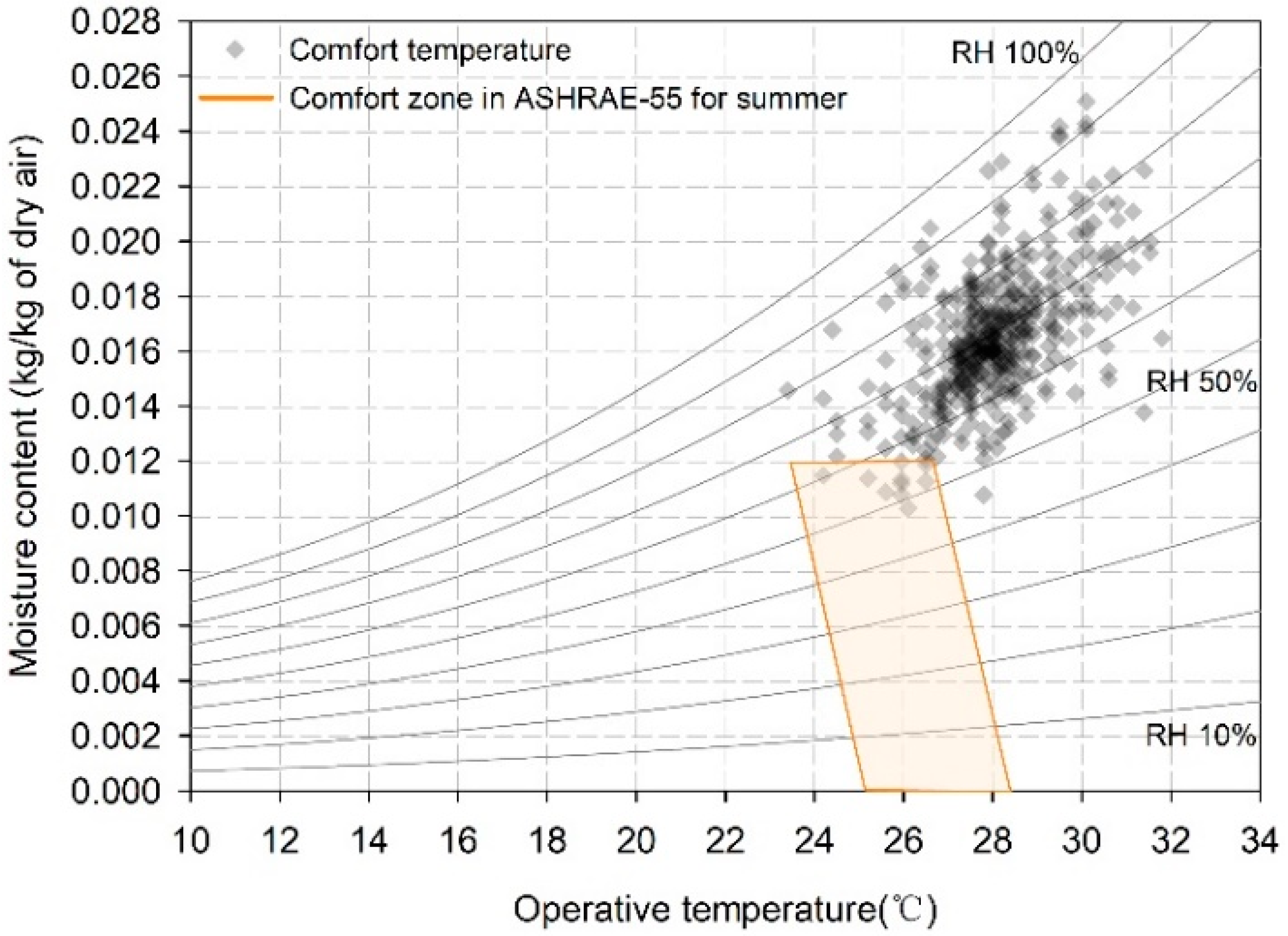
In office buildings with ECS in Urumqi during the summer season, the variations of indoor air temperatures were mainly distributed from 26 °C to 30 °C with the relative humidity remaining at a higher level (60–90%). Mean air velocity was under 0.2 m/s for more than half of the time.

(2)

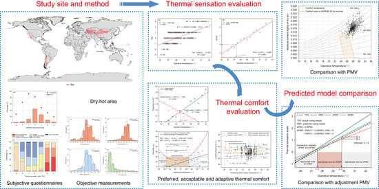
Although over 40% of the occupants could accept the current environment, there was still a willingness among them for it to be slightly cooler, which indicated that the deviation existed between thermal neutrality and expectation. The expectative temperature (T_e) was 26.6 °C, approximately 0.7 °C lower than the neutral temperature (T_n) of 27.3 °C. The upper limit of 80% acceptable interval for APD was 30.3 °C, 1.9 °C higher than that calculated by PPD.

(3)

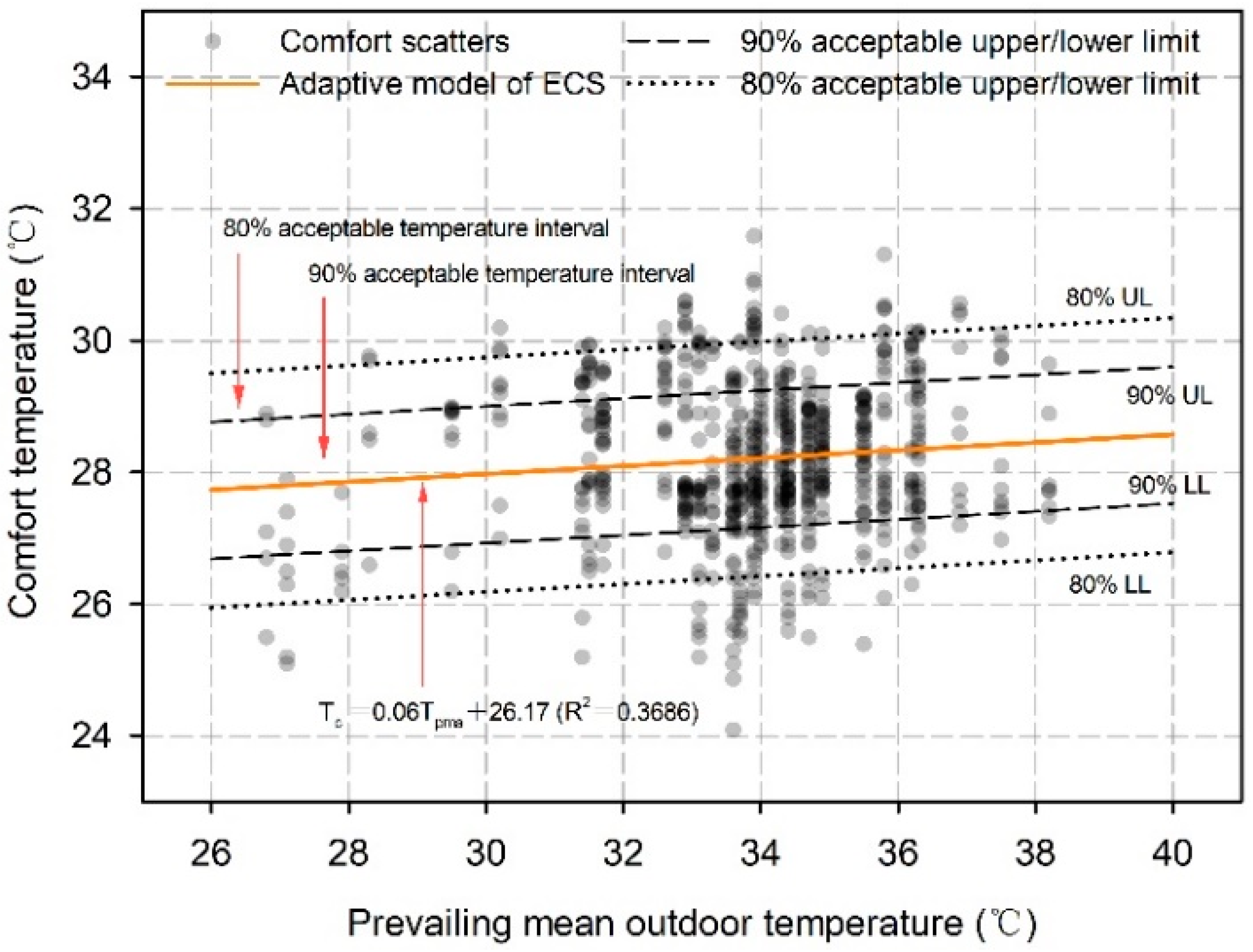
Due to the close relationship between comfort temperature and outdoor climatic conditions, an adaptive thermal comfort model was established for ECS office buildings. Based on the coupling effects of subjects’ behavioral habits, psychological preference and physiological accommodation, the specific mathematical equation could be expressed as T_c = 0.06T_pma + 26.17 (26.8 °C ≤ T_pma ≤ 38.2 °C). In addition, the comfort interval for the 90% and 80% acceptable levels were further obtained at 27.1–28.9 °C and 26.4–30.3 °C, respectively.

(4)

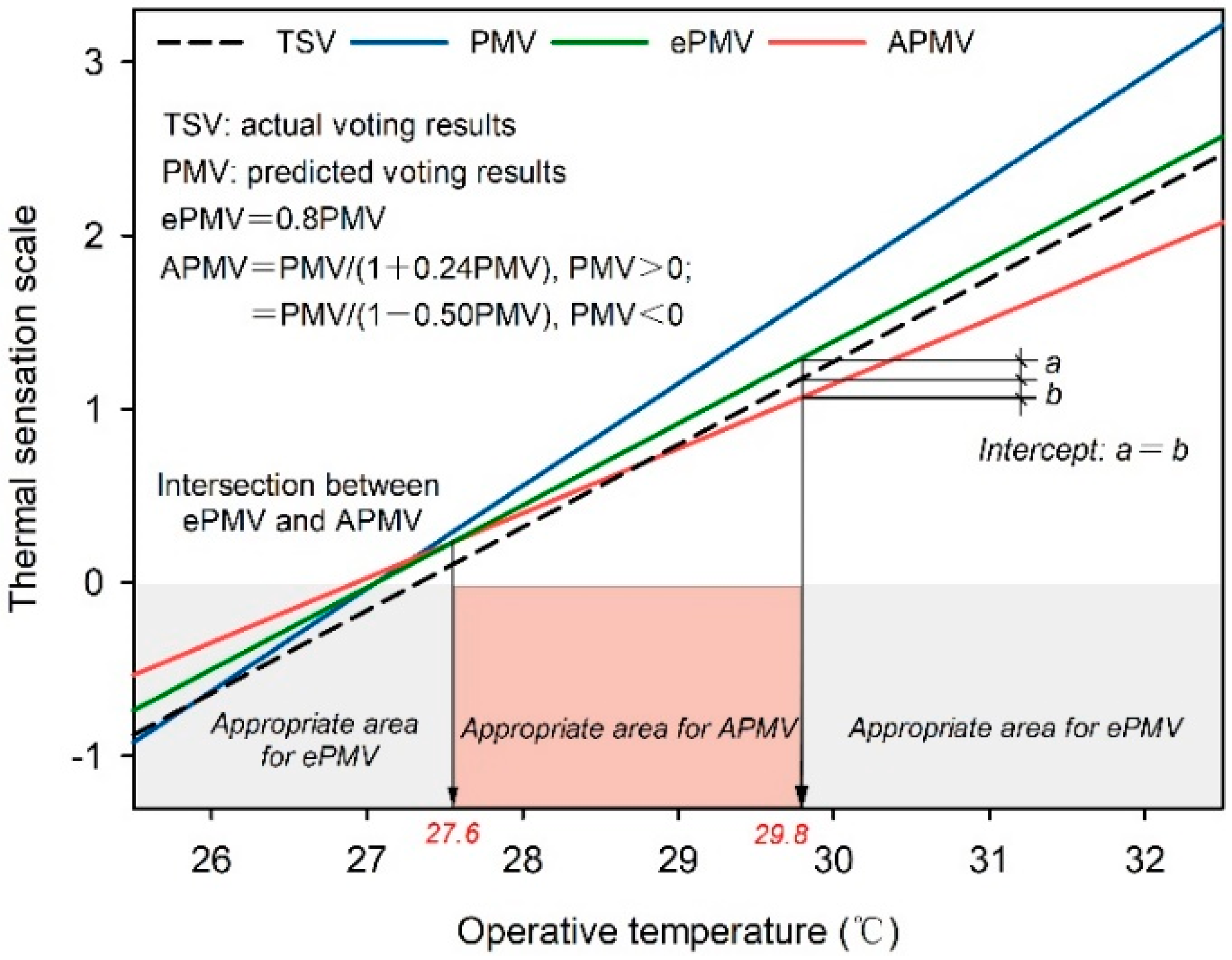
PMV had been proven not applicable for evaluating the actual thermal sensation in ECS office buildings due to its underestimation of subjects’ heating tolerance in summer. Meanwhile, by quantitating the adjustment PMV model can receive the optimal usage interval for ePMV and APMV of T_op < 27.6 °C/T_op > 29.8 °C, and 27.6 °C < T_op < 29.8 °C, respectively.

(5)

By comparing with previous studies on different indoor working modes, it can be observed that the neutral temperature (T_n) in ECS office buildings was basically higher than AC and MM modes, and lower than the NV mode. This was mainly attributed to the occupants’ various behavioral adjustments and thermal history in Urumqi.

Above all, through the exploration in this study, one can maintain actual thermal sensation under the background of cleaner and sustainable energy. Meanwhile, taking the difference analysis with conventional working conditions could further improve the quality of the indoor environment. Additionally, it should make full use of the occupants’ thermal adaptability under the specific environment to appropriately elevate the indoor design temperature in summer, so as to provide reference values for the revision of local energy-saving standards.

References

1. CHN. China Building Energy Efficiency Annual Development Report; Building Energy Conservation Research Center: Beijing, China; Tsinghua University: Beijing, China, 2016. [Google Scholar]
2. Yang, L.; Yan, H.Y.; Lam, J.C. Thermal comfort and building energy consumption implications—A review. Appl. Energy 2014, 115, 164–173. [Google Scholar] [CrossRef]
3. Guo, Y.; Bart, D. Optimization of design parameters for office buildings with climatic adaptability based on energy demand and thermal comfort. Sustainability 2020, 12, 3540. [Google Scholar] [CrossRef]
4. Osterman, E.; Tyagi, V.V.; Butala, V.; Rahim, N.A.; Stritih, U. Review of PCM based cooling technologies for buildings. Energy Build. 2012, 49, 37–49. [Google Scholar] [CrossRef]
5. Pérez-Lombard, L.; Ortiz, J.; Pout, C. A review on buildings energy consumption information. Energy Build. 2008, 40, 394–398. [Google Scholar] [CrossRef]
6. Xuan, Y.M.; Xiao, F.; Niu, X.F.; Huang, X.; Wang, S.W. Research and application of evaporative cooling in China: A review (I)–Research. Renew. Sustain. Energy Rev. 2012, 16, 3535–3546. [Google Scholar] [CrossRef]
7. Watt, J.R.; Brown, W.K. Evaporative Air Conditioning Handbook, 3rd ed.; The Fairmont Press: Lilburn, GA, USA, 1997. [Google Scholar]
8. Huang, X.; Liu, M. Study of evaporative cooling application condition in Xinjiang area of China. Refri. Air Condi. 2001, 1, 33–38. (In Chinese) [Google Scholar]
9. ANSI/ASHRAE 55–2020; Thermal Environmental Conditions for Human Occupancy. American Society of Heating, Refrigerating and Air-Conditioning Engineers, Inc.: Peachtree Corners, GA, USA, 2020.
10. EN ISO 7730; Ergonomics of the Thermal Environment: Analytical Determination and Interpretation of Thermal Comfort Using Calculation of the PMV and PPD Indices and Local Thermal Comfort Criteria. International Organization for Standardization: Geneva, Switzerland, 2005.
11. E. CEN 15251; Indoor Environment Input Parameters for Design and Assessment of Energy Performance of Buildings Addressing Indoor Air Quality, Thermal Environment, Lighting and Acoustics. European Committee for Standard: Brussels, Belgium, 2007.
12. Gibse, G.A. Environmental Design; The Chartered Institution of Building Services Engineers: London, UK, 2006. [Google Scholar]
13. Fanger, P.O. Analysis and Applications in Environmental Engineering; Danish Technical Press: Copenhagen, Denmark, 1970. [Google Scholar]
14. Humphreys, M.A.; Nicol, J.F. Understanding the adaptive approach to thermal comfort. ASHRAE Trans. 1998, 104, 991–1004. [Google Scholar]
15. De Dear, R.J.; Brager, G.S. Thermal comfort in naturally ventilated buildings: Revisions to ASHRAE standard 55. Energy Build. 2002, 34, 549–561. [Google Scholar] [CrossRef] [Green Version]
16. Tewari, P.; Mathur, S.; Mathur, J.; Kumar, S.; Loftness, V. Field study on indoor thermal comfort of office buildings using evaporative cooling in the composite of India. Energy Build. 2019, 199, 145–163. [Google Scholar] [CrossRef]
17. Bravo, G.; Gonzalez, E. Thermal comfort in naturally ventilated spaces and under indirect evaporative passive cooling conditions in hot-humid climate. Energy Build. 2019, 63, 79–86. [Google Scholar] [CrossRef]
18. Fu, C.; Mak, C.M.; Fang, Z.; Oladokun, M.O.; Zhang, Y.; Tang, T. Thermal comfort study in prefab construction site office in subtropical China. Energy Build. 2020, 217, 109958. [Google Scholar] [CrossRef]
19. Indraganti, M.; Ooka, R.; Rijal, H.B. Thermal comfort in offices in summer: Findings from a field study under the ‘setsuden’ conditions in Tokyo, Japan. Build. Environ. 2013, 61, 114–132. [Google Scholar] [CrossRef]
20. Hwang, R.L.; Lin, T.P.; Kuo, N.J. Field experiments on thermal comfort in campus classrooms in Taiwan. Energy Build. 2006, 38, 53–62. [Google Scholar] [CrossRef]
21. Liu, Y.; Rong, F.; He, W.; He, Q.; Yan, L. Adaptive thermal comfort and climate responsive building design strategies in dry-hot and dry-cold areas: Case study in Turpan, China. Energy Build. 2019, 209, 109678. [Google Scholar]
22. Jiao, Y.; Yu, H.; Yu, Y.; Wang, Z.; Wei, Q. Adaptive thermal comfort models for homes for older people in Shanghai, China. Energy Build. 2020, 215, 109918. [Google Scholar] [CrossRef]
23. Zhang, Y.; Wang, J.; Chen, H.; Zhang, J.; Meng, Q. Thermal comfort in naturally ventilated buildings in hot-humid area of China. Build. Environ. 2010, 45, 2562–2570. [Google Scholar] [CrossRef]
24. Tse, J.M.Y.; Jones, P. Evaluation of thermal comfort in building transitional spaces–Field studies in Cardiff, UK. Build Environ. 2019, 156, 191–202. [Google Scholar] [CrossRef] [Green Version]
25. Ming, R.; Yu, W.; Zhao, X.; Liu, Y.; Li, B.; Essah, E.; Yao, R. Assessing energy saving potentials of office buildings based on adaptive thermal comfort using a tracking-based method. Energy Build. 2020, 208, 109611. [Google Scholar] [CrossRef]
26. Wu, Z.; Li, N.; Wargocki, P.; Peng, J.; Li, J.; Cui, H. Field study on thermal comfort and energy saving potential in 11 split air-conditioned office buildings in Changsha, China. Energy 2019, 182, 471–482. [Google Scholar] [CrossRef]
27. Martin, E.; Lissen, J.M.S.; Martin, J.G.; Ruiz, P.; Brotas, L. Field study on adaptive thermal comfort in mixed mode office buildings in southwestern area of Spain. Build Environ. 2017, 1323, 30277–30279. [Google Scholar]
28. Zhou, L.; Li, N.; He, Y.; Peng, J.; Wang, C.; Yongga, A. A field survey on thermal comfort and energy consumption of traditional electric heating devices (Huo Xiang) for residents in regions without central heating systems in China. Energy Build. 2019, 196, 134–144. [Google Scholar] [CrossRef]
29. Wu, T.; Cao, B.; Zhu, Y. A field study on thermal comfort and air-conditioning energy use in an office building in Guangzhou. Energy Build. 2018, 168, 428–437. [Google Scholar] [CrossRef]
30. Wang, Z.; Li, A.; Ren, J.; He, Y. Thermal adaptation and thermal environment in university classrooms and offices in Harbin. Energy Build. 2014, 77, 192–196. [Google Scholar] [CrossRef]
31. Jiang, J.; Wang, D.; Liu, Y.; Di, Y.; Liu, J. A field study of adaptive thermal comfort in primary and secondary school classrooms during winter season in Northwest China. Build. Environ. 2020, 175, 106802. [Google Scholar] [CrossRef]
32. Lv, J.; Jing, J.; Fu, Y.; Liu, H. Experimental and numerical study of a multi-unit evaporative cooling device in series. Case Stud. Therm. Eng. 2020, 21, 100727. [Google Scholar] [CrossRef]
33. Xuan, Y.M.; Xiao, F.; Niu, X.F.; Huang, X.; Wang, S.W. Research and applications of evaporative cooling in China: A review (Ⅱ)–Systems and equipment. Renew. Sustain. Energy Rev. 2012, 16, 3523–3534. [Google Scholar] [CrossRef]
34. CHN GB50178–1993; Standard of Climatic Regionalization for Architecture. China Planning Press: Beijing, China, 1993.
35. Kottek, M.; Grieser, J.; Beck, C.; Rudolf, B.; Rubel, F. World map of the Köppen-Geiger climate classification updated. Mete Zeit 2006, 15, 259–263. [Google Scholar] [CrossRef]
36. CHN GB50176–2016; Code for Thermal Design of Civil Building. China Planning Press: Beijing, China, 2016.
37. Dhaka, S.; Mathur, J.; Wagner, A.; Agarwal, G.D.; Garg, V. Evaluation of thermal environmental conditions and thermal perception at naturally ventilated hostels of undergraduate students in composite climate. Build. Environ. 2013, 66, 42–53. [Google Scholar] [CrossRef]
38. Kant, K.; Kumar, A.; Mullick, S.C. Space conditioning using evaporative cooling for summers in Delhi. Build. Environ. 2001, 36, 1–11. [Google Scholar] [CrossRef]
39. EVS-EN ISO 7726; Ergonomics of the Thermal Environments–Instruments for Measuring Physical Quantities. ISO: Geneva, Switzerland, 2003.
40. Yang, L.; Yan, H.Y.; Mao, Y.; Yang, Q. The basis of climatic adaption for human thermal comfort. J. Sci. Press 2017, 79–80. (In Chinese) [Google Scholar]
41. Griffiths, I.D. Thermal Comfort in Building with Passive Solar Features: Field Studies; Commission of the European Communities: London, UK, 1991. [Google Scholar]
42. Griffiths, I.D. Thermal Comfort in Buildings with Passive Solar Features: Field Studies; EN3S-090 Report to the Commission of the European Communities; Commission of the European Communities: London, UK, 1990. [Google Scholar]
43. Hwang, R.L.; Cheng, M.J.; Lin, T.P.; Ho, M.C. Thermal perceptions, general adaptation methods and occupant’s idea about the trade-off between thermal comfort and energy saving in hot-humid regions. Build. Environ. 2009, 44, 1128–1134. [Google Scholar] [CrossRef]
44. Kumar, S.; Mathur, J.; Mathur, S.; Singh, M.K.; Loftness, V. An adaptive approach to define thermal comfort zone on psychrometric chart for naturally ventilated buildings in composite climate of India. Build. Environ. 2016, 109, 135–153. [Google Scholar] [CrossRef] [Green Version]
45. Thapa, R.; Rijal, H.B.; Shukuya, M. Field study on acceptable indoor temperature in temporary shelters built in Nepal after massive earthquake 2015. Build. Environ. 2018, 135, 330–343. [Google Scholar] [CrossRef]
46. Damiati, S.A.; Zaki, S.A.; Rijal, H.B.; Wonorahardjo, S. Field study on adaptive thermal comfort in office buildings in Malaysia, Indonesia, Singapore, and Japan during hot and humid season. Build. Environ. 2016, 109, 208–223. [Google Scholar] [CrossRef]
47. Singh, M.K.; Mahapatra, S.; Atreya, S.K. Thermal performance study and evaluation of comfort temperatures in vernacular buildings of North-East India. Build Environ. 2010, 45, 320–329. [Google Scholar] [CrossRef]
48. Humphreys, M.A.; Nicol, J.F.; Roaf, S. Adaptive Thermal Comfort: Foundations and Analysis; Routledge: London, UK, 2016. [Google Scholar]
49. Rijal, H.B.; Yoshida, H.; Umemiya, N. Seasonal and regional differences in neutral temperatures in Nepalese traditional vernacular houses. Build Environ. 2010, 45, 2743–2753. [Google Scholar] [CrossRef]
50. Villadiego, K.; Velay-Dabat, M.A. Outdoor thermal comfort in a hot and humid climate of Colombia: A field study in Barranquilla. Build Environ. 2014, 75, 142–152. [Google Scholar] [CrossRef]
51. Li, B.; Zheng, J.; Yao, R.; Jing, S. Indoor Thermal Environment and Human Thermal Comfort; Chongqing University Press: Chongqing, China, 2012. (In Chinese) [Google Scholar]
52. Nicol, J.F.; Humphreys, M.A. Adaptive thermal comfort and sustainable thermal standards for buildings. Energy Build. 2002, 34, 563–572. [Google Scholar] [CrossRef]
53. De Dear, R.J.; Brager, G.; Cooper, D. Developing an adaptive model of thermal comfort and preference. ASHRAE Trans. 1997, 104, 145–167. [Google Scholar]
54. Fanger, P.O.; Toftum, J. Extension of the PMV model to non-air-conditioned buildings in warm climates. Energy Build. 2002, 34, 533–536. [Google Scholar] [CrossRef]
55. Yao, R.; Li, B.; Liu, J. A theoretical adaptive model of thermal comfort–adaptive predicted mean vote (aPMV). Build Environ. 2009, 44, 2089–2096. [Google Scholar] [CrossRef]
56. CHN GB/T50785–2012; Evaluation Standard for Indoor Thermal Environment in Civil Buildings. Chongqing University: Chongqing, China, 2012.
57. Zhang, Z.; Zhang, Y.; Khan, A. Thermal comfort of people in a super high-rise building with central air-conditioning system in the hot-humid area of China. Energy Build. 2020, 209, 109727. [Google Scholar] [CrossRef]
58. Indraganti, M.; Boussaa, D. An adaptive relationship of thermal comfort for the Gulf Cooperation Council (GCC) Countries: The case of offices in Qatar. Energy Build. 2018, 159, 201–212. [Google Scholar] [CrossRef]
59. López-Pérez, L.A.; Flores-Prieto, J.J.; Ríos-Rojas, C. Adaptive thermal comfort model for educational buildings in a hot-humid climate. Build. Environ. 2019, 150, 181–194. [Google Scholar] [CrossRef]
60. Ricciardi, P.; Buratti, C. Thermal comfort in open plan offices in northern Italy: An adaptive approach. Build. Environ. 2012, 56, 314–320. [Google Scholar] [CrossRef]
61. Rijal, H.B.; Humphreys, M.A.; Nicol, J.F. Towards an adaptive model for thermal comfort in Japanese offices. Build. Res. Inf. 2017, 45, 717–729. [Google Scholar] [CrossRef]
62. Indraganti, M.; Ooka, R.; Rijal, H.B. Field investigation of comfort temperature in Indian office buildings: A case of Chennai and Hyderabad. Build. Environ. 2013, 65, 195–214. [Google Scholar] [CrossRef]
63. Dhaka, S.; Mathur, J.; Brager, G.; Honnekeri, A. Assessment of thermal environmental conditions and quantification of thermal adaptation in naturally ventilated buildings in composite climate of India. Build. Environ. 2015, 86, 17–28. [Google Scholar] [CrossRef] [Green Version]
64. Singh, M.K.; Ooka, R.; Rijal, H.B.; Takasu, M. Adaptive thermal comfort in the offices of north-east India in autumn season. Build. Environ. 2017, 124, 14–30. [Google Scholar] [CrossRef]
65. Thapa, S.; Bansal, A.K.; Panda, G.K. Thermal comfort in naturally ventilated office buildings in cold and cloudy climate of Darjeeling, India–An adaptive approach. Energy Build. 2018, 160, 44–60. [Google Scholar] [CrossRef]
66. Rupp, R.F.; de Dear, R.J.; Ghisi, E. Field study of mixed-mode office buildings in southern Brazil using an adaptive thermal comfort framework. Energy Build. 2018, 158, 1475–1486. [Google Scholar] [CrossRef]
Figure 1. Climate classification and selection of sites.
Buildings 12 01827 g001
Figure 2. Annual meteorological parameters of Urumqi.
Buildings 12 01827 g002
Figure 3. Photographs of the field investigation process.
Buildings 12 01827 g003
Figure 4. The distribution of indoor thermal environmental parameters: (a) air temperature; (b) globe temperature; (c) relative humidity; (d) air velocity.
Buildings 12 01827 g004
Figure 5. The results of subjective questionnaires: (a) thermal sensation vote and thermal acceptability; (b) distribution of thermal expectative vote in each TSV interval; (c) distribution of overall comfort vote in each TSV interval.
Buildings 12 01827 g005aBuildings 12 01827 g005b
Figure 6. Regression analysis between operative temperature and thermal sensation vote: (a) initial data; (b) binned data.
Buildings 12 01827 g006
Figure 7. The frequency distribution of Griffiths neutral temperature (G = 0.5).
Buildings 12 01827 g007
Figure 8. Regression analysis of expectative temperature.
Buildings 12 01827 g008
Figure 9. Acceptable temperature interval determined by APD and PPD.
Buildings 12 01827 g009
Figure 10. The intent frequency of behavioral adaptions.
Buildings 12 01827 g010
Figure 11. The relationship between operative temperature and clothing insulation.
Buildings 12 01827 g011
Figure 12. The relationship between operative temperature and metabolic rate.
Buildings 12 01827 g012
Figure 13. The relationship between indoor comfort temperature and prevailing mean outdoor temperature in summer.
Buildings 12 01827 g013
Figure 14. Comparison of comfort temperatures (this study) with recommended the comfort zone in ASHRAE-55 (PMV model) for summer.
Buildings 12 01827 g014
Figure 15. Comparison of TSV (this study) with previous adaptive predicted models.
Buildings 12 01827 g015