Development and Test of a New Fast Estimate Tool for Cooling and Heating Load Prediction of District Energy Systems at Planning Stage

Abstract

During the design and planning stage of a district energy system, the prediction of the cooling and heating loads is an important step. The accurate estimate of the load pattern can provide a basis for the configuration and optimization of the system. To meet the demand in practical application, this paper proposes a fast load prediction method for district energy systems based on a presimulated forward modelling database and KNN (K-nearest neighbor) algorithm and develops it into a practical tool. Owing to the absence of some design parameters at the planning stage, scenario analysis is also used to determine some input conditions for load prediction. In this paper, the scenarios cover three types of building: office, shopping mall and hotel. To test the performance of this new method, we randomly selected 15 virtual buildings (5 buildings for each type) with different design parameters and took their detailed BPS (building performance simulation) model as a benchmark to assess the prediction results of the new method. The index “ratio of the hours with effective prediction” is defined as the ratio of the hours whose relative error of hourly load prediction is less than 15% to the hours whose load is not 0 in the whole year, and the test result shows that this index is not less than 0.9 (90%) for the predicted cooling load of all 45 test cases and the predicted heating load of 25 of the 45 cases. As a research achievement with practical value, this paper accomplishes the programming work of the tool and makes it into a software. The application of this software in the actual project of district energy system is also presented. The performance of the new load prediction tool was compared with the traditional approach commonly used in engineering—the load estimation based on reference building models—and the result shows that the fast load estimate tool can provide the same level of prediction accuracy as traditional simulation methods.

1. Introduction

Human activities in urban areas will continuously consume a lot of energy and emit carbon dioxide and pollutants into the environment. For the sustainable development of the city and society, planners and engineers are committed to improving energy efficiency and reducing the environmental impact of energy production and consumption. A district energy system is a kind of proven solution that can meet the above demands. By definition, the district energy system refers to an integrated energy system that can solve the multiple energy requirements of human activities in a specific district (e.g., heating, cooling, hot water, gas and power supply, etc.). The “district” referred to can be an urban street block divided by administration, an industrial/research park, or a community with multiple types of buildings [1]. Through the rational planning, design and operation control of district energy systems, the efficient production, transmission, distribution and consumption of various forms of energy in cities can be realized. In addition, district energy systems can utilize many new energy technologies such as cogeneration, renewable energy and smart grids to further promote energy conservation and emission reduction [2]. At present, society is taking “carbon neutralization” as the goal of energy planning, which means that district energy systems will have a broader application prospect.

High-quality planning and design are the foundation of a successful district energy system. During the planning and design stage, the accurate prediction of community loads and energy demands can provide a reliable calculation basis for the configuration of the energy system [3]. The load prediction is also a significant step to further optimize the design of the system [4]. For example, load levelling, which refers to smoothing the load profile by reducing the difference between the on-peak and off-peak loads, is an effective technique to lower the operation cost and prolong the life cycle of the system [5]. The simplest and most convenient approach to estimate the load in engineering practice is to multiply the load intensity index per unit area by the building area. However, these “load indices” are mainly based on experiences and very likely to result in overestimation of loads; their values are static in the calculation, which means they cannot reflect the dynamic characteristics of loads on the annual scale [6]. In many application and research scenarios such as economic analysis or community load levelling, a prediction of the hourly loads of buildings is required. Although designers and engineers can calculate the hourly loads using BPS (building performance simulation) tools (e.g., eQuest, DeST, EnergyPlus, etc.) for a project at the planning and design stage [7], they need to collect sufficient geometric and physical information about the buildings, which is usually quite difficult in this preliminary stage of a project [8]. Thus, this paper proposes a new method to predict the hourly loads of buildings for district energy systems at the planning stage. To meet practical needs, this new method should ensure both the accuracy of the prediction and the convenience of use.

The loads of a district energy system refer to the superposition of the instantaneous loads of multiple buildings at the same time pace. Therefore, the load prediction of district energy can be divided into two main steps: load prediction for every individual building with different types and functions in the district; and the superposition and correction of multiple prediction results on the scale of cities or communities. For the former step, there have already been a lot of related studies. In 2012, Zhao and Magoules published a review on the prediction methods of building energy consumption and the proposal for future prospects [9]. At present, using BPS software is still the most commonly used method for the load prediction of individual buildings. For example, Han et al. predicted the annual and peak cooling load for several types of buildings based on the prototypical building models established with DeST [10]. Ourghi et al. proposed an approach to predict the annual energy consumption of office buildings by DOE-2 models, while the influence of building shape on cooling and heating loads was also considered [11]. Nihar et al. used an EnergyPlus model to predict the energy consumption of a building to realize the optimal control of the operable windows [12]. Lim and Zhai proposed a Monte Carlo simulation method combined with EnergyPlus modelling to obtain the regression formula of the building energy consumption [13]. Zhu et al. also used the stochastic modelling method based on EnergyPlus models to predict the cooling and heating loads of buildings at the planning stage [14]. However, modellers can only establish the BPS models on a case-by-case basis, which is not very convenient to the nonprofessional users in practice. Another common load prediction method is the statistical method based on monitoring data [15]. Many types of data-driven model, such as multiple nonlinear regression [16], time series [17], artificial neural network (ANN) [18], support vector machine (SVM) [19] and grey-box models [20], have been successfully applied to the load prediction for a single building. It can be seen that an accurate prediction result will be obtained based on correct detailed building information (for the simulation method) or sufficient monitoring data (for the statistical method).

The latter step is the superposition of the predicted results of multiple individual buildings in space and time on the district scale. Researchers have independently completed some related studies in decades. For example, Chow et al. used DOE-2 models to predict the cooling load of a new community for the optimal design of the district cooling system [21]. Shimoda et al. established a series of detailed building models to predict the energy consumption and CO2 emissions at the city scale [22]. Ren et al. created a prototypical building model database and used it to predict the end-use electricity consumption in a residential area [23]. The data-driven model has also been applied in the load prediction of a district energy system, although a larger scale of data is required than the individual building. Warnken et al. used the regression model method to forecast the sector-wide building energy consumption of the tourism accommodation industry in Australia [24]. Jiang et al. used the ANN model to predict the hourly cooling loads for a community with a district cooling system based on the annual monitoring data [25]. Wan et al. established a correlation model of cooling/heating loads and weather parameters using the principal component analysis method [26]. Shamshirband et al. utilized the adaptive neuro-fuzzy algorithm to predict district heating loads [27]. Al-Shammari et al. trained a data-driven model that combines SVMs with FFA to predict the loads of a district heating system [28]. Ferracuti et al. analysed three types of data-driven models for the load prediction in real buildings and found that they can show good accuracy at short-term prediction periods [29]. In sum, the statistical methods are more suitable for the buildings or district energy systems in operation instead of the planning and design phase due to the requirement for the monitoring data of loads.

In recent year, the concept of “UBEM (urban building energy modelling)” has gradually attracted the attention of academic and engineering communities [30]. Urban energy planning is one of very important domains of applications of UBEM. Some bottom-up physical-based UBEM tools have had the function of guiding the planning and design of district energy systems, such as CityBES, OpenIDEAS, CEA, URBANopt, TEASER, etc. [31]. Some other scholars also reviewed the statistical methods used for UBEM [32] or established the data-driven framework for UEUM (urban energy use modelling) by case studies [33], which both reveal that big data is a very important part and one of the future trends in the development of UBEM. However, there is still a slight deviation from the focus of UBEM tools and the requirement of district load prediction in practice. Now, a major challenge of UBEM is the shortage of computing resources [34]. Therefore, the analysis of a single building is usually simplified in many UBEM tools, which is reasonable on the urban scale. As the object of district energy planning, the scale of a community is much smaller than that of a city, and planners often need more accurate load prediction data; in addition, in many actual planning projects, the available building information is limited, and the relevant staff are likely to be nonprofessional in modelling and simulation. Therefore, it is necessary to develop a load prediction tool that can strike a balance between convenience and accuracy to better meet the actual needs of engineers.

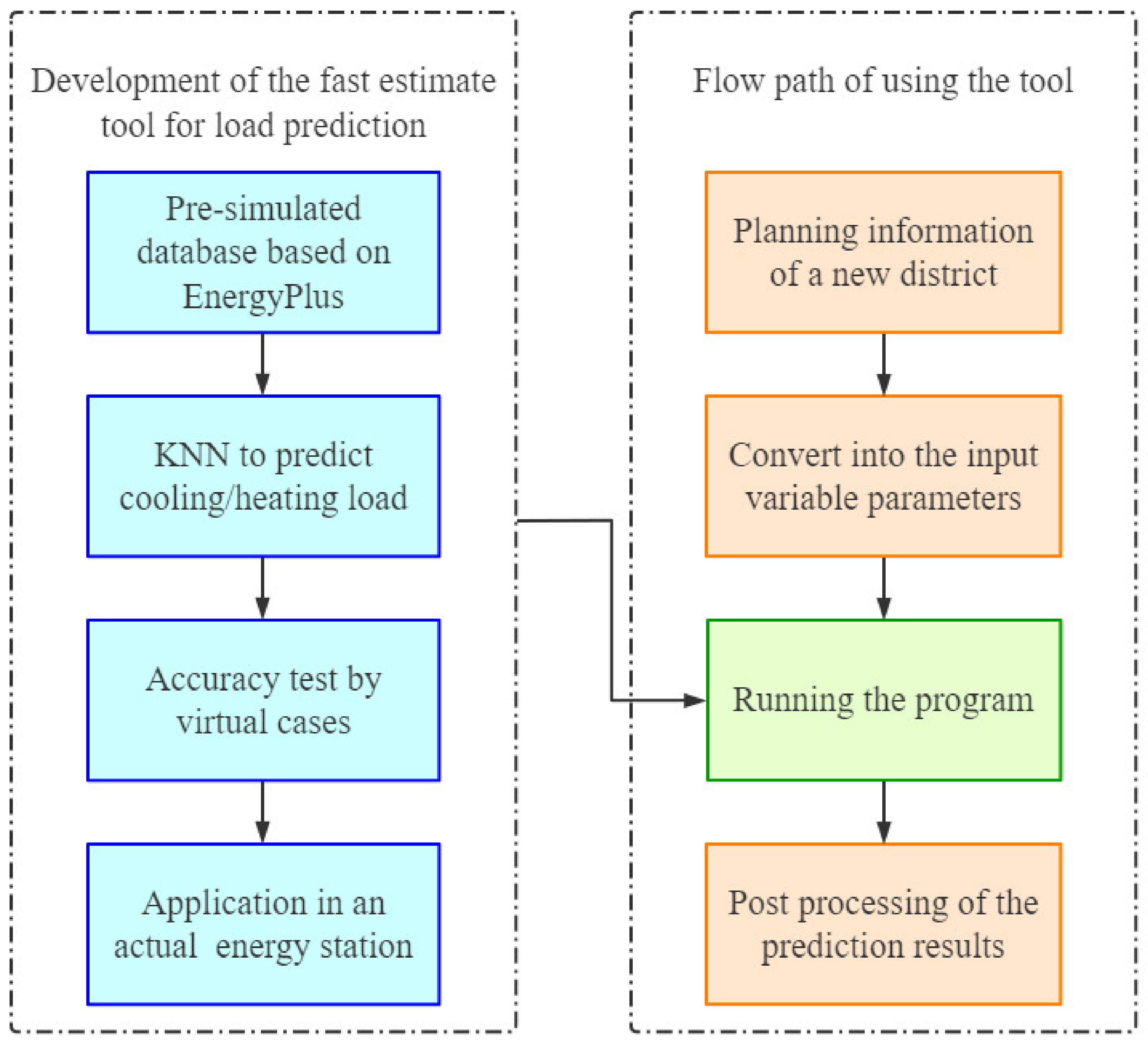
This paper proposes a fast load prediction method for district energy systems based on a presimulated building model database and KNN (K-nearest neighbor) algorithm. In general, a district energy system is usually an integrated system combined with centralized heating, cooling and electricity supply to meet the demands of a specific district/community. On the scale of hourly time-step, the electricity load is relatively stable and periodic throughout the whole year, but the cooling and heating loads have a strong correlation with the state of indoor environment and outdoor climate. Thus, the method proposed in this paper is only aimed at the prediction of cooling and heating loads. The novelty of this method is to provide a new idea of utilizing a large number of forward simulation models and machine learning technology (KNN) to develop a practical tool for cooling/heating load prediction at the planning stage of district energy systems. The decision makers who are not professional in BPS can easily use this tool to perform load prediction in actual projects without a tedious modelling process, but with guaranteed accuracy.

2. Methodology

The specific research methodology of this study is as follows (Figure 1):

(1)

Establishment of a forward modelling database: As the foundation of this study, we used EnergyPlus to establish a large number (5625) of BPS models. Each model corresponds to a design scenario of new buildings and all models form a database that can cover most scenarios of buildings in district energy planning.

(2)

Development of the KNN-algorithm-based method for load prediction: According to the planning information of the new community, the total building area of each design scenario in the district can be determined. For every single scenario, this paper proposes a new approach to predict the hourly specific cooling and heating load per building area of the whole year based on a machine learning method: the KNN algorithm. In this approach, the building model database established in Step (1) is used as the data source for KNN algorithm. This new method is finally developed into a practical fast estimate tool for cooling and heating load prediction in regional energy planning.

(3)

Accuracy test of the tool: We firstly randomly generated 15 different building models (5 offices, 5 shopping malls and 5 hotels). The scenario analysis of this study covers 3 different scenarios for each type of building. Therefore, these 15 virtual buildings were arranged and combined with 3 design scenarios, and then 45 test cases could be totally obtained. For each case, we used two methods to accomplish the load prediction: simulation method based on BPS models and the new method developed in this paper. The simulation results of the detailed building models were selected as the baseline of the predicted value; since a detailed BPS model can generate the simulation data with enough accuracy for the load prediction at the design stage, these data are regarded as the baseline for the new load prediction method proposed in this paper to be compared with. The difference (relative error) between the results of these two methods are used as the index to evaluate the accuracy of the fast estimate tool.

(4)

Development of the software and the application in an actual project: The tool is developed into a software with graphic UIs by Python and QtDesigner. To present how to apply the software in an actual project, an actual application case is also conducted in this paper. The fast estimate tool is used to predict the cooling and heating load of a new community at the planning stage of Shanghai West Hongqiao energy station. After the energy station is put into operation, the annual measurement data of cooling and heating for the object community are utilized to verify the accuracy of the predicted result made at the planning stage, which can show the effectiveness of the load prediction tool in practice.

The following parts of this chapter will give the details of the main work to be conducted in (1) and (2).

2.1. Presimulated Building Model Database

2.1.1. Settings of Model Parameters

The load estimate method developed in this study is based on KNN algorithm. To train the machine learning model, sufficient data should be prepared in advance. In this paper, we establish a presimulated BPS model database to generate a large amount of hourly load data. Every model in the presimulated database has a unique set of parameters, which means they correspond to a building with a unique design scenario. In order to ensure the applicability of the database under different design conditions, the parameters of the models in the database should be set in an appropriate way: the values of the input variables to predict the loads should be available at the planning and design stage, while the value ranges of these variables should cover most of the scenes that may appear in reality. This subsection will introduce the detailed settings of the model parameters in the database.

To be a useful tool in practice, a concise and clear UI (user interface) is required. Users can import the planning information from the UI. This means that the load prediction tool is such a function: to output 8760 hourly cooling and heating loads of a whole year with this input information. Thus, the database should provide the training data in the same format. The variable parameters of the models in the database correspond to the input variables on the UI, while the presimulation results of these models correspond to the output loads. This section will first introduce the settings of the input variables and the variable model parameters. As listed in

Table 1. Input variables on the UI of the load prediction tool.

Item Name	Subitem Name	Range or Options
(1) Location (City)		Shanghai
(2) Geometric parameters	(2a) Length/width/height	>0 m
	(2b) Total floor area	>0 m2
	(2d) Number of floors	>0
(3) Building type		Office, shopping mall and hotel
(4) Envelope	(4a) Area ratio of window to wall	0.1~0.7
	(4b) Exterior wall/window/roof with compliant heat transfer coefficient	Yes
	(4c) Exterior window with compliant solar heat gain coefficient (SHGC)	Yes
(5) Scenario type		3 scenarios for each building type
(6) Probability for the scenario		0~1

, the input variables on the UI are determined based on the actual situation of energy planning project.

Then, the parameter settings of the models in the database can be determined according to this input variable list. In

Table 2. Parameter settings of the building models in database.

Class	Item	Setting
Meteorological Parameters	(1) Annual hourly weather data	The typical meteorological year (TMY) file of Shanghai
Geometric parameters	(2) Shape factor [m−1]	0.12/0.16/0.2/0.24/0.28
	(3) Area ratio of the southward projected to the total side surface (ARST)	0.25/0.28/0.31/0.34/0.37
	(4) Floor height [m]	3/3.5/4/4.5/5
	(5) Number of floors	3
Envelope parameters	(6) U-value of exterior wall/window/roof	See Table 3
	(7) SHGC of exterior window	See Table 3
	(8) Area ratio of window to wall (ARWW)	0.1/0.25/0.4/0.55/0.7
Indoor Conditions	(9) Lighting power density	See Table 4
	(10) Plug equipment power density	See Table 4
	(11) Occupant density	See Table 4
	(12) Volume of fresh air [m2/(h·p)]	30
	(13) Indoor design temperature	See Figure 3 and Figure 4
Other parameters	(14) Building type	Office/shopping mall/hotel
	(15) Schedule	See Figure 5, Figure 6 and Figure 7 and Table 5

, the parameter settings of the main factors that affect the cooling and heating load of the building are clearly shown. Part of the model parameters that corresponds to the input information from the users is variable (5 levels of values for each variable parameter), and part of the others remains unchanged in all the models in the database. In the following paragraphs, the setting of each model parameter will be introduced in detail.

To predict 8760 hourly cooling and heating loads of the building, the annual hourly weather data are required. In the presimulation of the building models in the database, the TMY file of the city where the project is located should be used. The tool developed in this paper only focuses on the application in Shanghai, so the TMY file of Shanghai for EnergyPlus was used to generate the simulation results of the database. If this tool needs to be applied for the projects in another city, a new database should be presimulated with the TMY file of this city. The approach to establish the presimulated BPS model database is universal.

The geometric parameters are the main part of the input information. In general, designers would basically determine the length, width, height, number of floors and total area of the building in the new community during the planning phase. These parameters can describe the approximate shape of the building, while supposing that the new building is a rectangular cylinder and ignoring some unimportant details. However, the variation of these parameters and the cooling/heating loads does not show an immediate correlation (for example, a linear positive correlation). Thus, some other geometric parameters that influence the loads directly should be used for the construction of the model database. Based on the existing related research [35], the following three variables are selected as the variable geometric parameters: shape factor (S), area ratio of the southward projection surface to the total side surface (ARST, α), and floor height (h_f).

Shape factor refers to the ratio of the external surface area of building in contact with ambient environment to the volume it encloses. The impact of shape factor on building loads is very significant. A larger shape coefficient expresses a larger specific external surface area per unit floor area. This will result in more heat transfer through the envelope, which means that the cooling and heating load of buildings will be larger. Another variable parameter is ARST, which reflects the aspect ratio and the orientation of buildings. The larger the proportion of southward projection area, the more heat the building gains, which will lead to a larger cooling load and a smaller heating load. Moreover, the floor height is also selected as a variable model parameter to determine the 3D shape of the building model (only 2 variables are not enough for the determination of a 3D model).

To simplify the modelling process, all models in the database have only 3 floors. These simplified building models are used to output the hourly specific cooling and heating load per unit floor area of top floor, middle floor and bottom floor, respectively. The database model that corresponds to the actual building is the model with the same length, width and floor height, except that the numbers of floors are different (arbitrary number for the actual building but 3 floors for the database model, as shown by Figure 2), and the actual specific load can be calculated by the presimulation results of the corresponding database model (Equation (1)):

$$L_t=L_{tf}+\left(n_f-2\right)L_{mf}+L_{bf}$$

(1)

where L_t refers to the total specific (cooling or heating) loads per unit floor area of the building (W/m²); L_tf, L_mf, and L_bf refer to the specific (cooling or heating) loads per unit floor area of the top floor, the middle floor and the bottom floor, respectively (W/m²); and n_f refers to the number of floors in the actual building.

The correlation between the three selected variable model parameters (S, α and h_f) and the original input information from users is determined by the following simultaneous equations based on geometric laws (Equation (2)):

$$\left\{\begin{array}{c}S=\frac{2\left(l+w\right)h^{\prime }+lw}{lw{h}^{\prime }}\\ \alpha =\frac{l{h}^{\prime }}{2\left(l+w\right)h^{\prime }}\\ h_f=\frac{h}{n_f}=\frac{h^{\prime }}{3}\end{array}\right.\stackrel{solving}{\Rightarrow } \left\{\begin{array}{c}l=\frac{2h^{\prime }}{\left(1-2\alpha \right)\left(\mathrm{S}{h}^{\prime }-1\right)}\\ w=\frac{h^{\prime }}{\alpha \left(\mathrm{S}{h}^{\prime }-1\right)}\\ h^{\prime }=3h_f\end{array}\right.$$

(2)

where l, w and h refer to the length, width and height of the building from the original input information, respectively (m); h’ refers to the height of the building model in the database (m). Note that the shape factor (α) in this paper refers to the shape factor of the model in the database rather than that of the actual building.

Based on Equation (2), the variable parameters for load prediction and the 3D size of the building can be converted to each other. This system of equations is used to determine the precise size of the model for the establishment of the presimulated model database. For example, supposing that the three variable geometric parameters are at the third level (S = 0.2, α = 0.31, h_f = 4 m), the geometry size of this case should be 45 m/28 m/12 m (length/width/height), and the modeller can easily build the model in EnergyPlus by referring to these size data. On the other hand, these equations are also used to convert the input geometric information from the UI into S, α and h_f. Since these parameters can directly influence the cooling and heating load, they will be utilized in KNN algorithm to realize the load prediction. A detailed introduction will be presented in Section 2.1.2.

The thermal property of envelope also affects the heat gain/loss of the building. These parameters can be important variables for BPS with detailed models, whereas their values are often still uncertain during the planning phase since the materials and the insulation measures are not determined at such a preliminary stage of the project. For this fast estimate tool, all parameters about the thermal property of envelope are set according to the current code for design of building energy efficiency (as shown in

Table 3. Envelope parameters of the building models in database.

Item	Unit	Value
(1) Heat transfer coefficient of exterior wall	W/(m2·K)	0.8
(2) Heat transfer coefficient of roof	W/(m2·K)	0.5
(3) Heat transfer coefficient of exterior window	W/(m2·K)	2.5
(4) SHGC of exterior window (northward)		0.4
(5) SHGC of exterior window (others)		0.35

) [36]. In practical use, the thermal parameters of envelope are not required except for the area ratio of window to wall; for different buildings, the value of this parameter varies widely, and unlike other thermal parameters of building materials, the value of the area ratio of window to wall (ARWW) can be approximately determined in the preliminary design scheme at the planning stage. Therefore, this parameter is selected as the variable parameter in the database models.

The parameters of indoor conditions that can affect the cooling and heating load include lighting power density, plug equipment power density, occupant density and indoor temperature set-points in summer and winter. On an hourly scale, these parameters basically change within a period of one day. Thus, they should be set in the form of “benchmark value + daily schedule”. The design standard for energy efficiency of public buildings in China provides the recommended values of these schedules in the computation of hourly cooling and heating load [36]. The benchmark values should be set by reference to the design scenario of the building. In this study, the load prediction tool provides 3 scenarios for each type of building for users to select in the scenario analysis.

Table 4. Benchmark values of indoor condition parameters in database.

Building Type	Scenario No.	Lighting Power Density [W/m2]	Plug Equipment Power Density [W/m2]	Occupant Density [m2/p]
Office	1	11	20	4
	2	18	13	8
	3	9	15	10
Shopping mall	1	12	13	3
	2	19	13	4
	3	10	13	8
Hotel	1	15	20	15
	2	15	13	30
	3	7	15	25

shows the settings of the benchmark values corresponding to all scenarios. For the schedule settings, the daily variations are illustrated by Figure 3, Figure 4, Figure 5, Figure 6 and Figure 7, and

Table 5. Operation time for cooling and heating system.

Building Type	Cooling Period	Heating Period	Daily Operation Time
Office, weekdays	May~Sep	Nov~Mar	7:00~19:00
Office, weekends			-
Shopping mall			8:00~21:00
Hotel			0:00~24:00

presents the operation time for the cooling and heating system in the buildings.

A total of 5625 groups of parameter values can be obtained by arranging all the above variable parameters of the building models (5 × 5 × 5 × 5 × 3 × 3 = 5625, as illustrated by Figure 8). Each group of parameter values corresponds to a BPS model in the presimulated database. In other words, the database used in this paper should store the information about the parameters of 5625 building models and their simulation results. The next subsection will demonstrate the process to generate such a database in detail.

2.1.2. Generating Database

All the BPS models in the database are derived from a prototypical building model. The prototypical model is established by DesignBuilder. The variable parameters of this model are set as follows: shape factor is 0.15 m⁻¹; ARST is 0.25; floor height is 3 m; ARWW is 0.1; building type is office; and the No. of indoor condition scenarios is 1 (as illustrated by Figure 9). This model is the first case in the database, and it is noted as the No. 0 building. No. 1~No. 5624 building corresponds to other 5624 models with different parameter settings. The task to generate over 5000 building models is too difficult for manual modellers. To automate this process, the scripts of models that record the values of parameters can be changed by programs. Since the model file of EnergyPlus (.idf files) can be opened and edited as a text document, the automatic model generation process would be implemented by a program that can automatically modify and save text files. In this study, we used Python to write such a program.

Moreover, the running simulation of these models and the postprocessing of calculation results would be also implemented by programs in an automated way. The simulation is completed in a multiprocess way on an 8-core CPU, and 5625 models only take 3.6 h in total. The calculation results include 6 sequences of load values: the hourly specific cooling/heating load per unit floor area of the top floor, the middle floor and the bottom floor. Every sequence contains 8760 values. The amount of data is very large, so we have to use a professional database to store them. MySQL is used in this study, since MySQL is open source software and its function is enough for the development task of the load prediction tool.

MySQL is a kind of relational database management system. Relational database stores data in different tables instead of putting all data in a large warehouse, which increases the speed and flexibility. Therefore, the structure of the presimulated model database must follow the regulations of relational database. As shown in Figure 10, there are 5626 tables in the database in total: one general table and 5625 subtables. There are 5625 rows in the general table, and each row of data corresponds to a building, in which the 6 variable parameters (shape factor, ARST, floor height, ARWW, building type and indoor condition scenario) and the building No. are recorded. The load data are recorded in the subtables, and each subtable corresponds to a building and stores its calculation results (6 sequences in total, 8760 items in each sequence). A database for the load prediction tool applied in Shanghai was generated in this paper. For databases applied in other cities, it can be established with the same process.

2.2. Load Prediction Tool Based on KNN Algorithm

The load prediction tool developed in this study is based on KNN algorithm. KNN is a nonparametric learning algorithm in machine learning, which is often used in classification and regression. The principle is as follows: for data space X and Y, when there is a linear or approximately linear mapping relation between X and Y (f: X→Y), an arbitrary y in Y (the mapping point of x in X) can be obtained through the interpolation calculation of a point set {y’} (a set of the mapping point of x’, which are the nearest neighbor points of x in X) (as illustrated by Figure 11). When there are enough data samples in the sample space, KNN algorithm has high accuracy. The presimulated database provides 5625 data samples, which is adequate to reflect the mapping relationship between X (the variable model parameters) and Y (hourly cooling and heating loads) in this study.

The variable parameters in the load prediction tool should be divided into two categories: continuous parameter and discrete parameter. Building type and indoor condition scenarios are both discrete parameters, which means that they will not be involved in KNN algorithm. Other 4 continuous parameters constitute a 4-dimensional data space; the 5 levels in each dimension form a 4-dimensional hypercube, and the big hypercube is composed of 625 (5 × 5 × 5 × 5 = 625) small hypercubes. When the information of a new building is input, it can be positioned to a certain point in this data space. Then, KNN algorithm is used to search which hypercube this point is in and all the vertices of this hypercube. These vertices are the nearest neighbor of the prediction point, and the corresponding load data stored in the database of these neighbor points would be used for interpolation to compute the hourly loads of the prediction point. The specific steps are introduced as follows:

(1)

Convert the input information of the prediction building into 6 variable parameters (shape factor, ARST, floor height, ARWW, building type and indoor condition scenario) by Equation (2) given in Section 2.1. It can be regarded as a prediction point in the data space.

(2)

Determine the data points from the database values to form the sample space according to the values of two discrete parameters. For example, supposing that the building type and indoor condition scenarios of one case are office and No. 1, respectively, it means that only the building models in the database whose settings of these two parameters are the same should be used in the load prediction of this case.

(3)

Search the vertices of the smallest hypercube that embodies the prediction point. For other 4 continuous parameters, each of them represents one dimension of the 4-dimensional data space. In each dimension, the prediction point must fall between the two levels. By pairwise comparison, we can determine which two levels the prediction point is between in each dimension. For example, supposing that the coordinates of a prediction point are shape factor = 0.2 m⁻¹, ARST = 0.3, floor height = 3.8 m, ARWW = 0.5, the point is located in the following intervals at four dimensions: [0.19, 0.23] (shape factor), [0.28, 0.31] (ARST), [3.5, 4] (floor height), [0.4, 0.55] (ARWW). Through full arrangement, a total of 16 vertices of the hypercube can be easily determined.

(4)

Sometimes the prediction point is not located inside a hypercube, but in a cube of the hypercube exactly (the prediction point coincides with a level in 1 dimension), on a surface (coincides in 2 dimensions), an edge (coincides in 3 dimensions) or even at the vertex (coincides in all 4 dimensions) of the hypercube. In this situation, the vertices of the cube (or surface/edge/vertex) that the prediction point is located at are regarded as the nearest neighbor for KNN algorithm.

(5)

Compute the hourly specific cooling/heating loads by Equation (3). All 6 groups of 8760 hourly load values should be calculated individually, which means the computation would be performed 52,560 (8760 × 6 = 52,560) times. Finally, the loads of 4 types of floors are added together according to Equation (2) to output the results of the prediction point.

$$y=\frac{{{\displaystyle \sum }}_{i=1}^p\left\{{\left[\sqrt{{{\displaystyle \sum }}_{j=1}^4{\left({x^{\prime }}_{i,j}-x_j\right)}^2}\right]}^{-1}{y^{\prime }}_i\right\}}{{{\displaystyle \sum }}_{i=1}^p\left\{{\left[\sqrt{{{\displaystyle \sum }}_{j=1}^4{\left({x^{\prime }}_{i,j}-x_j\right)}^2}\right]}^{-1}\right\}}$$

(3)

where y refers to the value of prediction point in space Y (in this study, it refers to hourly specific cooling/heating load); y’_i refers to the value of the i-th nearest neighbor in space Y; x_j refers to the value of prediction point in space X at the j-th dimension (in this study, it refers to 4 variable parameters—shape factor, ARST, floor height and ARWW); x_i,j refers to the value of the i-th nearest neighbor in space X at the j-th dimension; and p refers to the number of nearest neighbors (the value takes 16, 8, 4, 2 or 1 in different conditions).

For the load prediction of district energy system at planning stage, this tool should be applied combined with scenario analysis. Here are the specific operation steps:

(1)

Determine the variable parameters of 3 types of building based on known planning information and output the prediction results of these buildings in all 3 design scenarios by the load prediction tool developed in this study.

(2)

Determine the probability for different scenarios occurs in 3 types of building by scenario analysis and carry out the weighted sum of the prediction results under 3 design scenarios is according to the probability for each type of building.

(3)

Calculate the total hourly cooling/heating load of the community according to planned building area of each type of building.

3. Test and Result

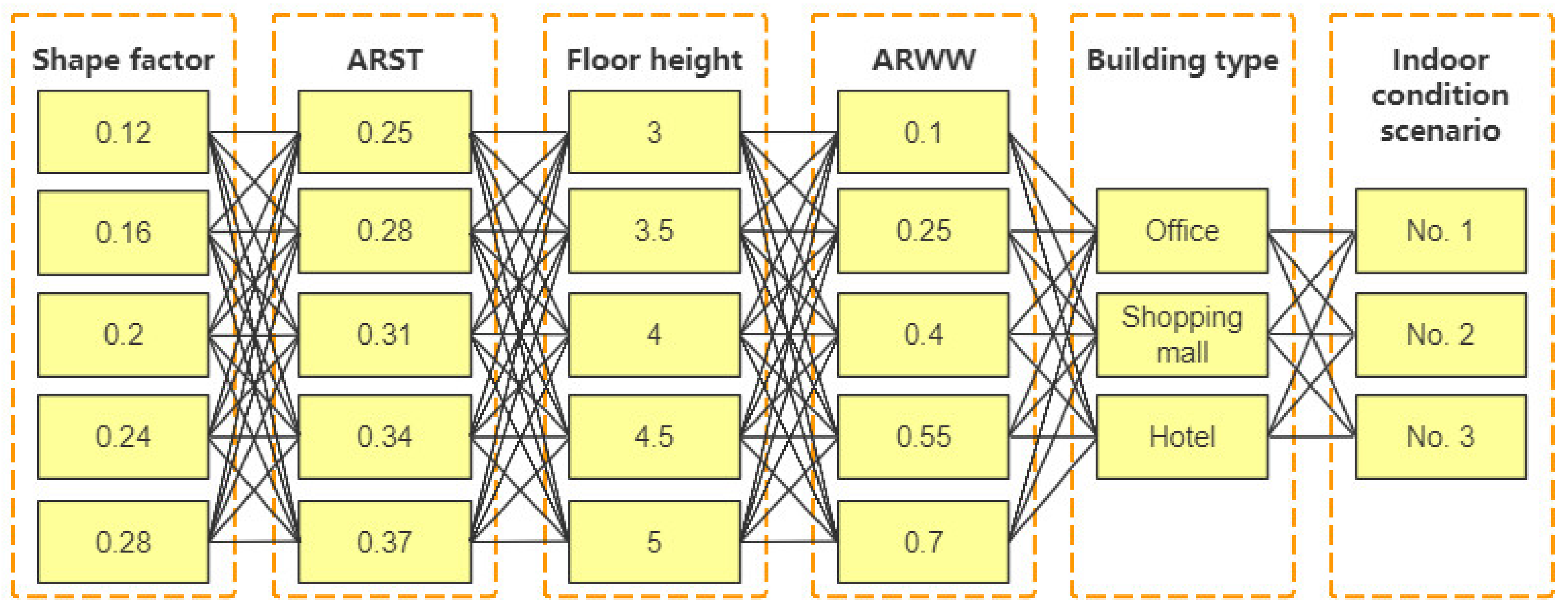
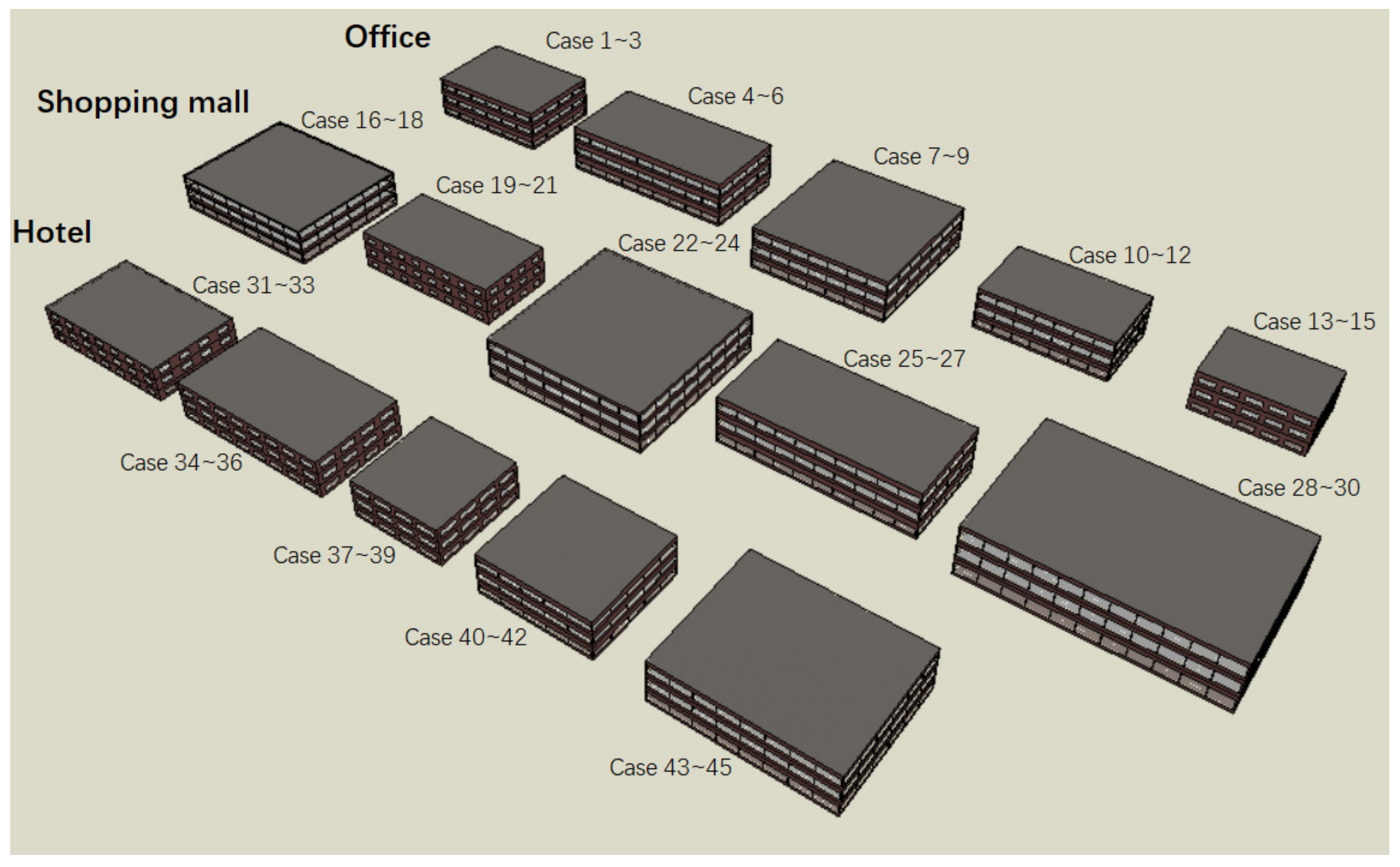
The developed tool requires a test to verify its accuracy and effectiveness. The test objects are 15 randomly generated BPS models with different input information. Among these 15 buildings, there are 5 of each type (office, shopping mall and hotel). For the sake of simplicity, the geometric parameters of the five models in each group are the same. In the load prediction tool, there are three kinds of settings to be chosen as the indoor condition scenarios for each type of building. Therefore, we arranged and combined these 15 virtual buildings with three different scenarios to create a total of 45 test cases. The model parameters of these test cases are presented in

Table 6. Model parameters of 45 test cases.

Building Type	Case No.	Shape Factor [m−1]	ARST	Floor Height [m]	ARWW	Indoor Condition Scenario
Office	1–3	0.220	0.292	4	0.35	No. 1~3
	4–6	0.194	0.333	4.5	0.4
	7–9	0.179	0.250	4.2	0.5
	10–12	0.230	0.310	4	0.5
	13–15	0.259	0.292	3.8	0.3
Shopping mall	16–18	0.197	0.281	3.5	0.6	No. 1~3
	19–21	0.231	0.328	3.6	0.2
	22–24	0.172	0.250	4	0.55
	25–27	0.193	0.338	4.5	0.45
	28–30	0.153	0.300	4.8	0.6
Hotel	31–33	0.238	0.313	3.2	0.25	No. 1~3
	34–36	0.220	0.321	3.5	0.3
	37–39	0.255	0.250	3.5	0.35
	40–42	0.226	0.259	3.8	0.4
	43–45	0.187	0.276	4	0.5

.

The development goal of the fast estimate tool for load prediction is to replace the detailed modelling method in the planning stage of a district energy system, improve the working efficiency without losing the accuracy of the prediction results and facilitate its use for nonprofessionals. This means that the simulation result of the detailed BPS model can be regarded as the baseline for the accuracy test of the tool. Thus, for all 45 of these test cases, their detailed BPS models are established in DesignBuilder (Figure 12) to output the baseline values, while the predicted values are also obtained by the fast load estimate tool. The difference (relative error) between the predicted and the baseline values presents the accuracy of the prediction results.

In the comparison between the prediction results and the baseline, a total of 8760 pairs of load values need to be compared with each other. Through preliminary observation of the prediction results, we find that the baseline and predicted loads are both very small in some hours. This may lead to a problem, in that the relative errors of these hours would be very large due to the small baseline value, although the absolute value of the gap between the baseline and the prediction is not big. 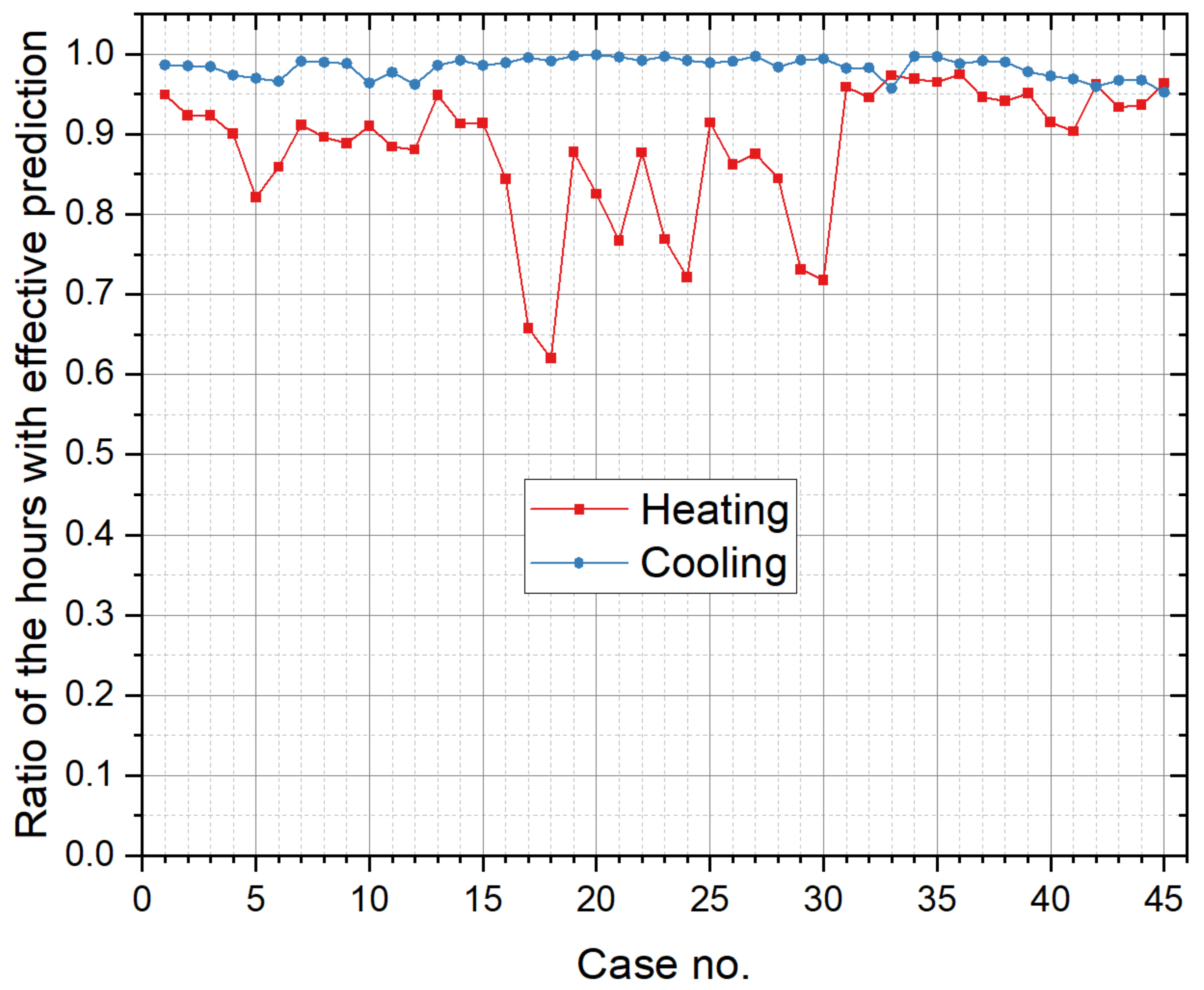For example, supposing that one of the baseline values of the cooling load is 1 W/m² and the predicted value is 1.5 W/m², the relative error would be very large (50%) in this hour. The aim of the development is to make the prediction results of the fast estimate tool close to the baseline value in the hours with significant cooling and heating loads, but this does not require benchmarking with the baseline value at every time. Therefore, a new index, “ratio of the hours with effective prediction”, is used to evaluate the accuracy of the prediction results on an annual scale. This index is defined as the ratio of the hours whose relative error of predicted load is less than 15% (referring to the requirement in ASHRAE Guideline [37]) to the hours with nonzero values of loads in the whole year. Moreover, the RE (relative error) of the peak value and the accumulated value of annual cooling and heating loads (equivalent to the cooling/heating energy consumed by the building during the whole year) are also computed as the test results.

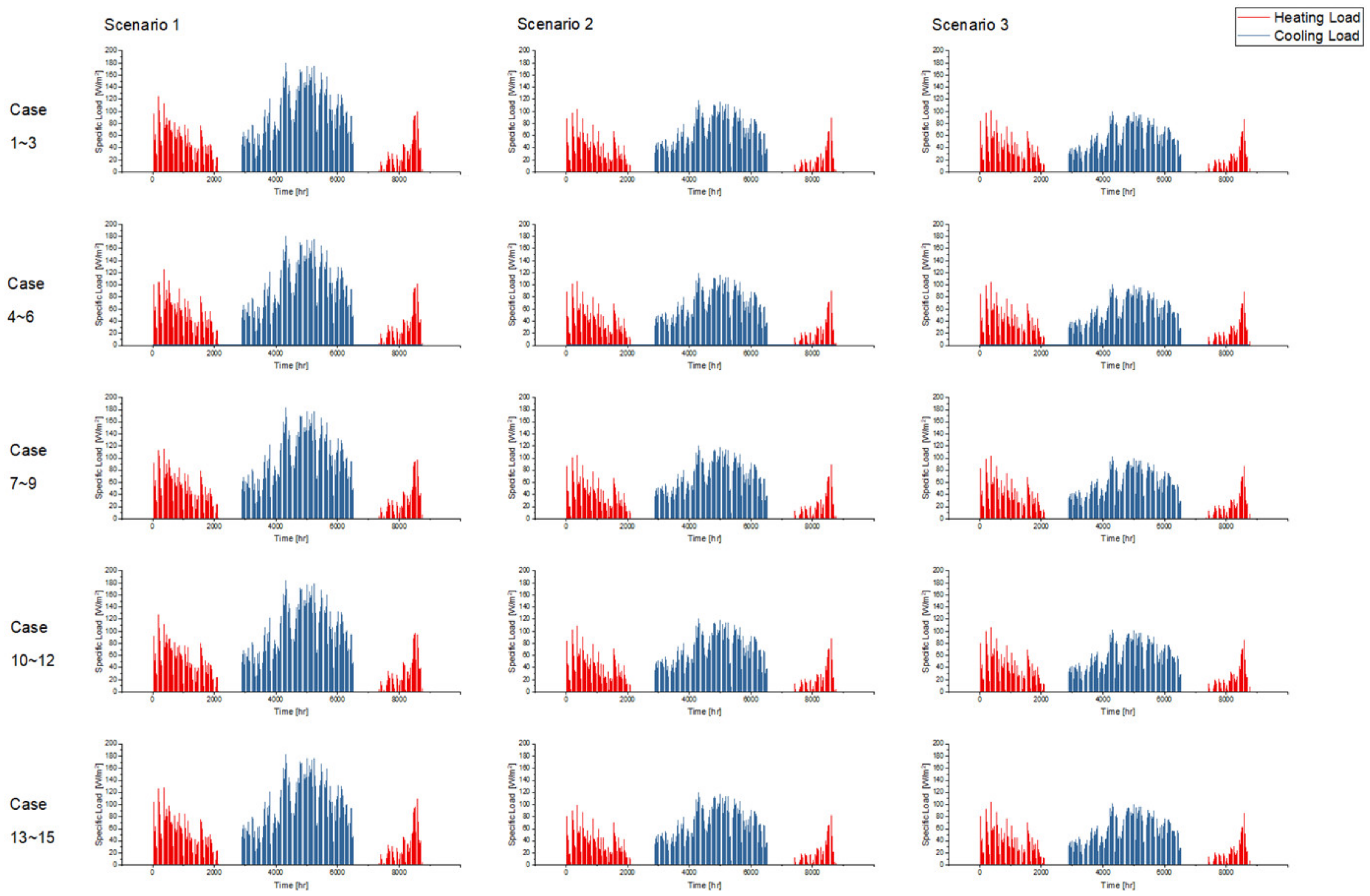
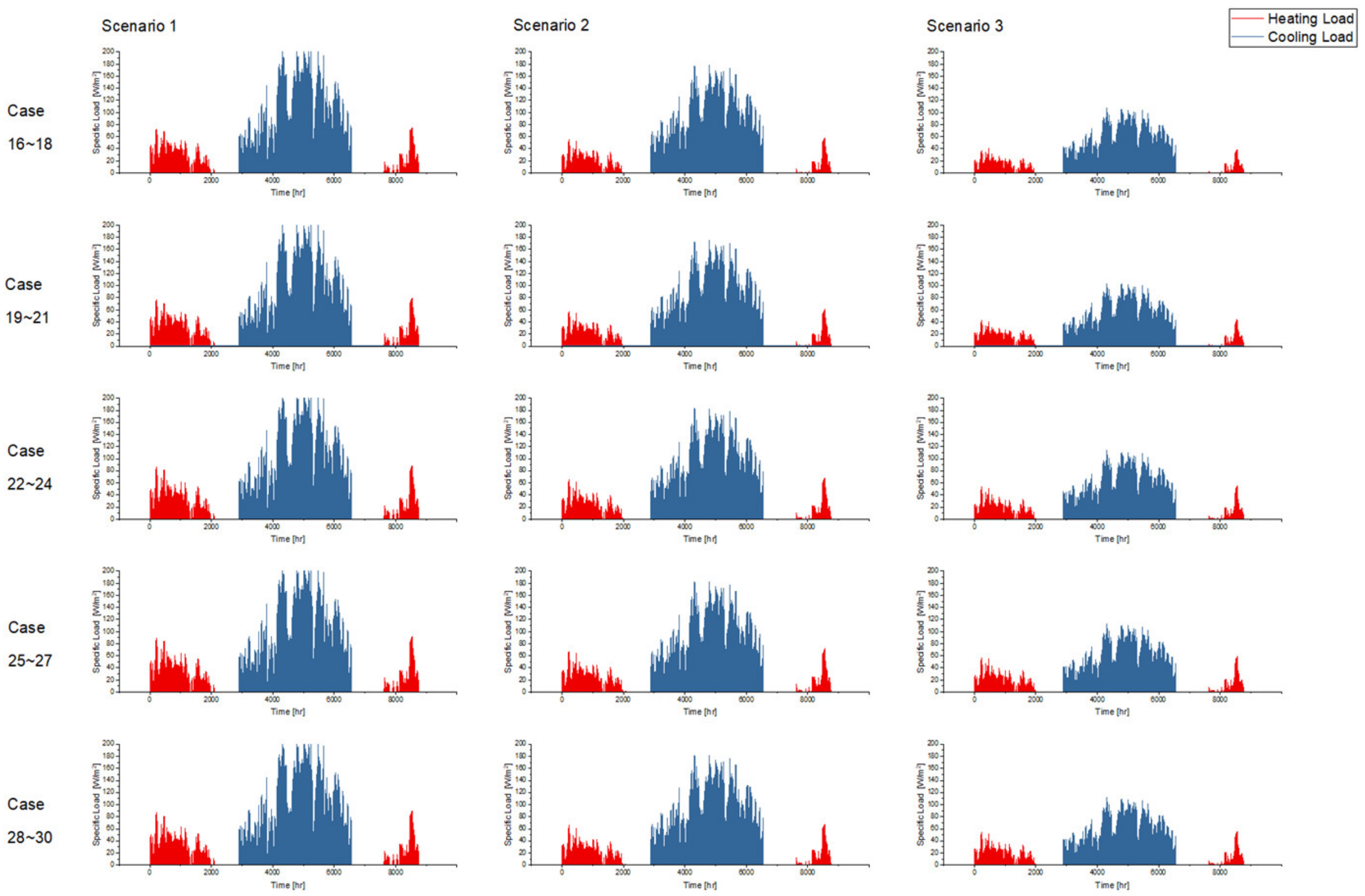
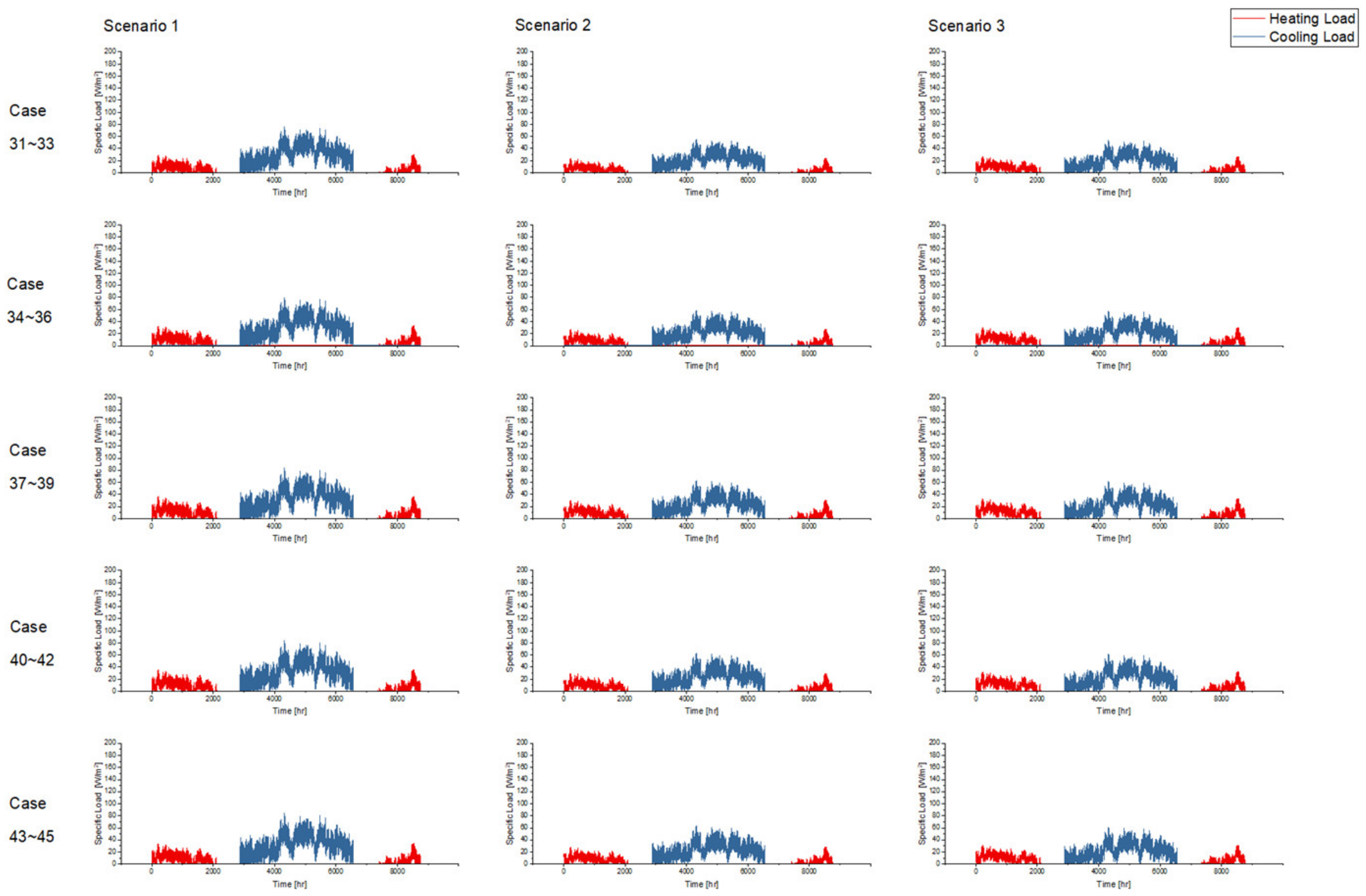
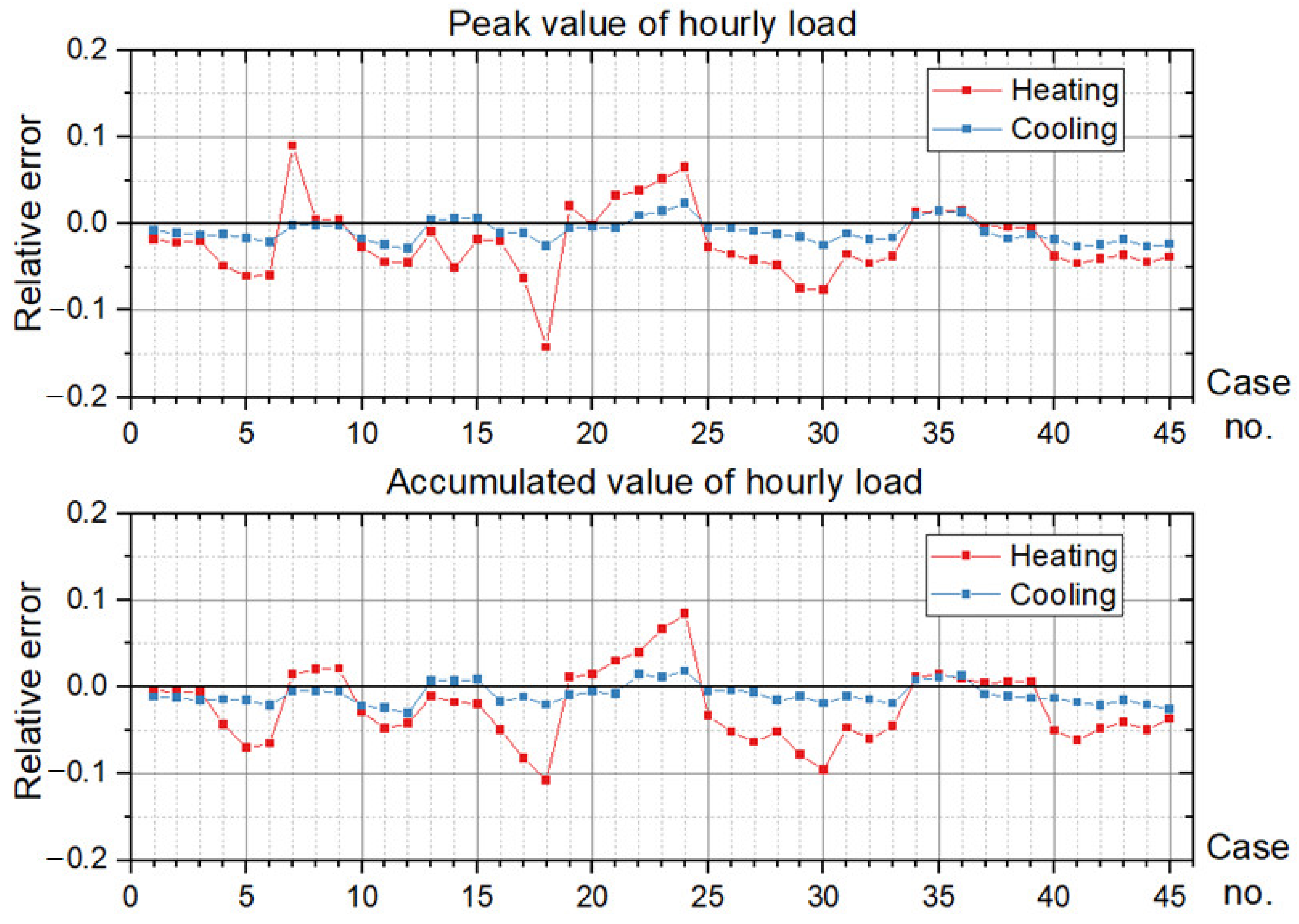
Figure 13, Figure 14 and Figure 15 illustrate the original prediction results of all the 45 cases. To show the overall condition of the prediction results, a line graph is used to illustrate the frequency distribution of “ratio of the hours with effective prediction” (Figure 16). Figure 17 presents the RE of the peak and the accumulated value of annual cooling and heating loads.

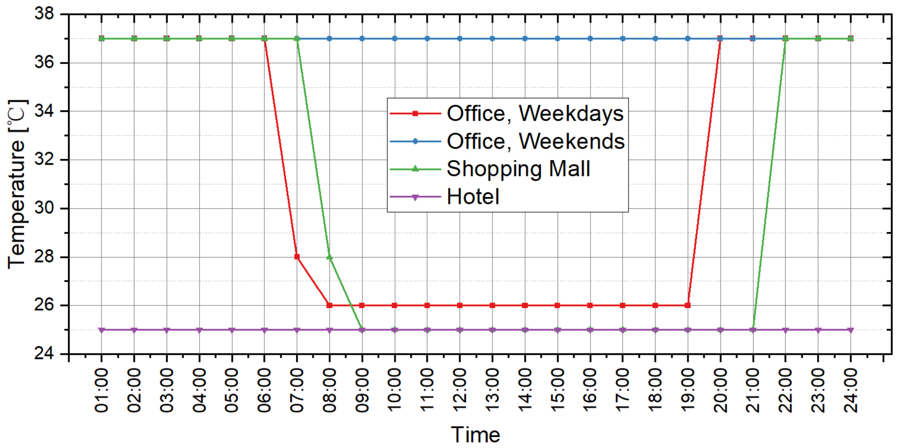
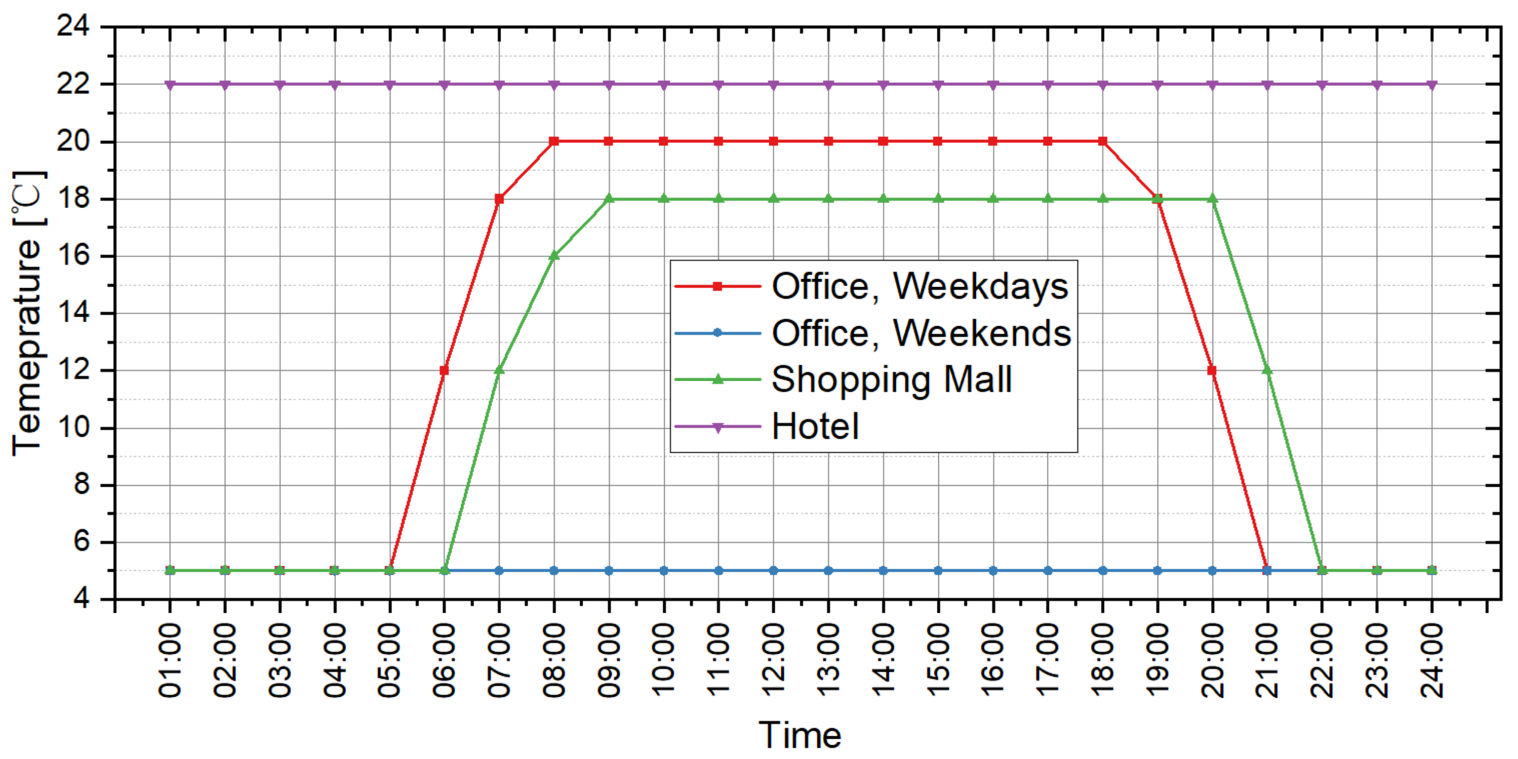
From the perspective of cooling load prediction, the test results of all cases are good: the “ratios of the hours with effective prediction” of the 45 test cases are higher than 0.95, which means that more than 95% of hours with nonzero cooling loads can be accurately predicted in all test cases; and the RE of the peak and the accumulated values of hourly load are both less than 0.05 in all test cases. This verifies that the method proposed in this paper has good performance in cooling load prediction. For heating load prediction, the test results show that the predictions of heating load in office and hotel cases (Cases 1~15 and Cases 31~45) are fairly good: the “ratio of the hours with effective prediction” is higher than 0.9 in most cases (25 of the 30 cases) and higher than 0.8 in all cases; the RE of the peak values of hourly load is less than 0.05 in 26 of the 30 cases and less than 0.1 in all cases; and the RE of the accumulated values of hourly load is less than 0.05 in 25 of the 30 cases and less than 0.1 in all cases. For the heating load prediction in the shopping mall cases (Cases 16~30), the accuracy is relatively worse than other cases on the scale of a single building: the “ratio of the hours with effective prediction” varies in the range of 0.6~0.95, and the RE of the peak and the accumulated values of hourly load are both less than 0.1 in all test cases except Case 18 (less than 0.15). According to the parameter settings of indoor conditions and operation schedules, the indoor design temperature in winter is relatively low (18 °C in shopping mall, 20 °C in office and 22 °C in hotel), and the occupancy density is relatively high. This results in the small absolute values of heating load in shopping malls, which leads to the poor performance of the indices that quantify the prediction accuracy. However, we can trust that this error will not cause a big bias for district energy planning since the error is still small in the terms of absolute values, although it is quite large in the terms of relative values. The application of the load prediction tool in an actual project of district energy planning, introduced in the next section, will confirm this view.

4. Application in an Actual Project

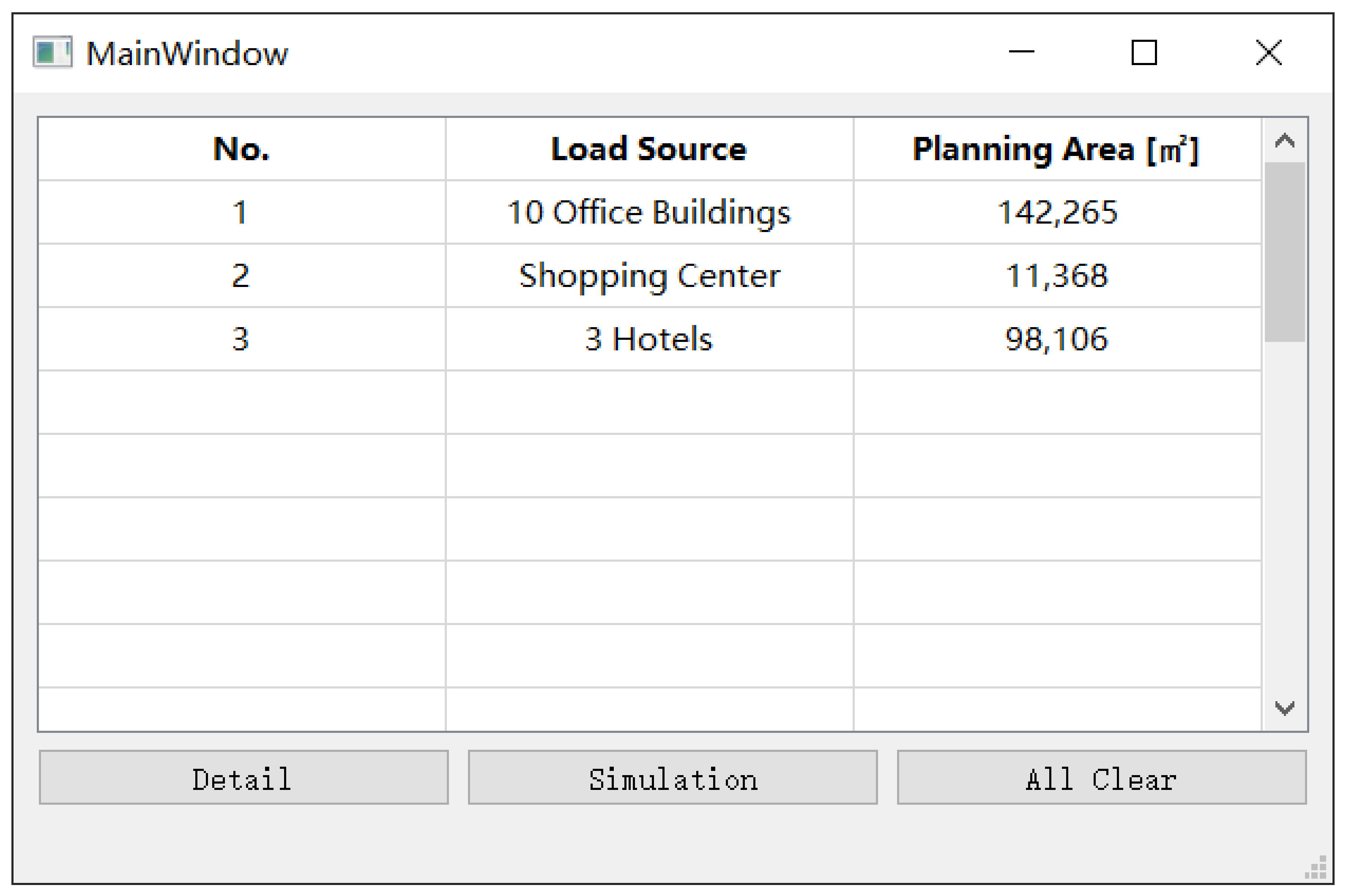
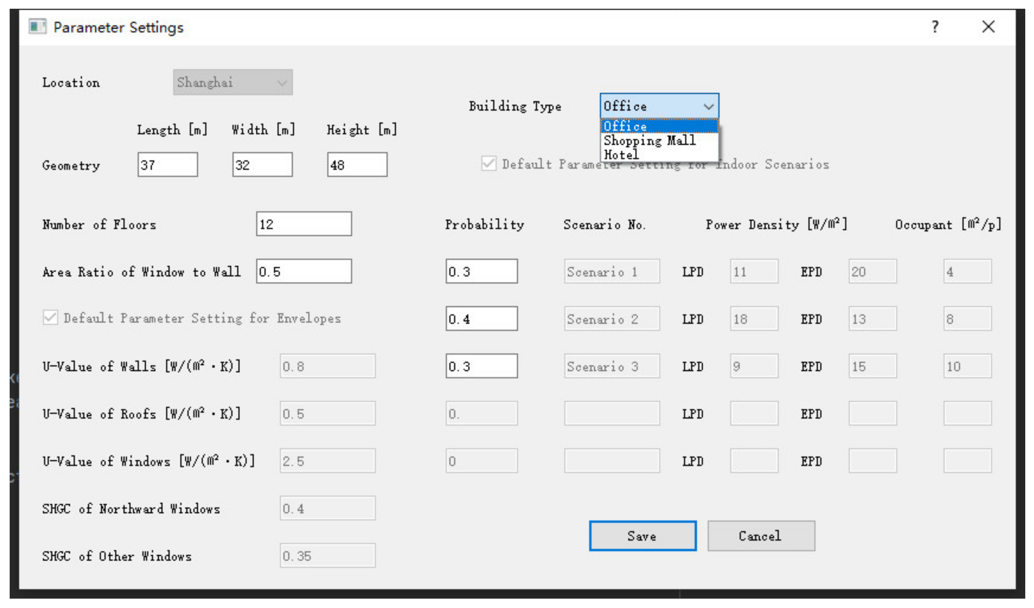
To make the research achievements practically valuable, we developed a fast estimate tool of load prediction with Python and QT Designer. The main UI is shown in Figure 18. In this software, users can set multiple types of load source (buildings) in the community as the input to predict the hourly cooling and heating loads for district energy planning. The maximum number of load sources is 20, and for each type of source, the detail parameter settings can be edited by clicking the “Detail” button with the table cell highlighted. The UI of detail parameter settings is as illustrated by Figure 19.

In this UI, users can input the length, width, height, the number of floors and the ARWW of the corresponding building to the highlighted load source. In the background of the software, the program will transfer the original geometric parameters (length, width and height) into the database parameters (shape factor, ARST and floor height). The building type for selection includes office, shopping mall and hotel, and after determining the building type, three default indoor scenarios will be displayed in the following boxes. At this time, the users need to input the probability of these scenarios. Obviously, some boxes in this UI are disable. For the parameter boxes of the envelopes and the indoor conditions, they are regarded as the constants for the application scenarios in this paper, so the values in these boxes are only used to exhibit the settings of the model parameters in the software. However, in further studies, we will expand the scale of the presimulated building model database to enable these values as the variable inputs. This provides an orientation for the software to upgrade.

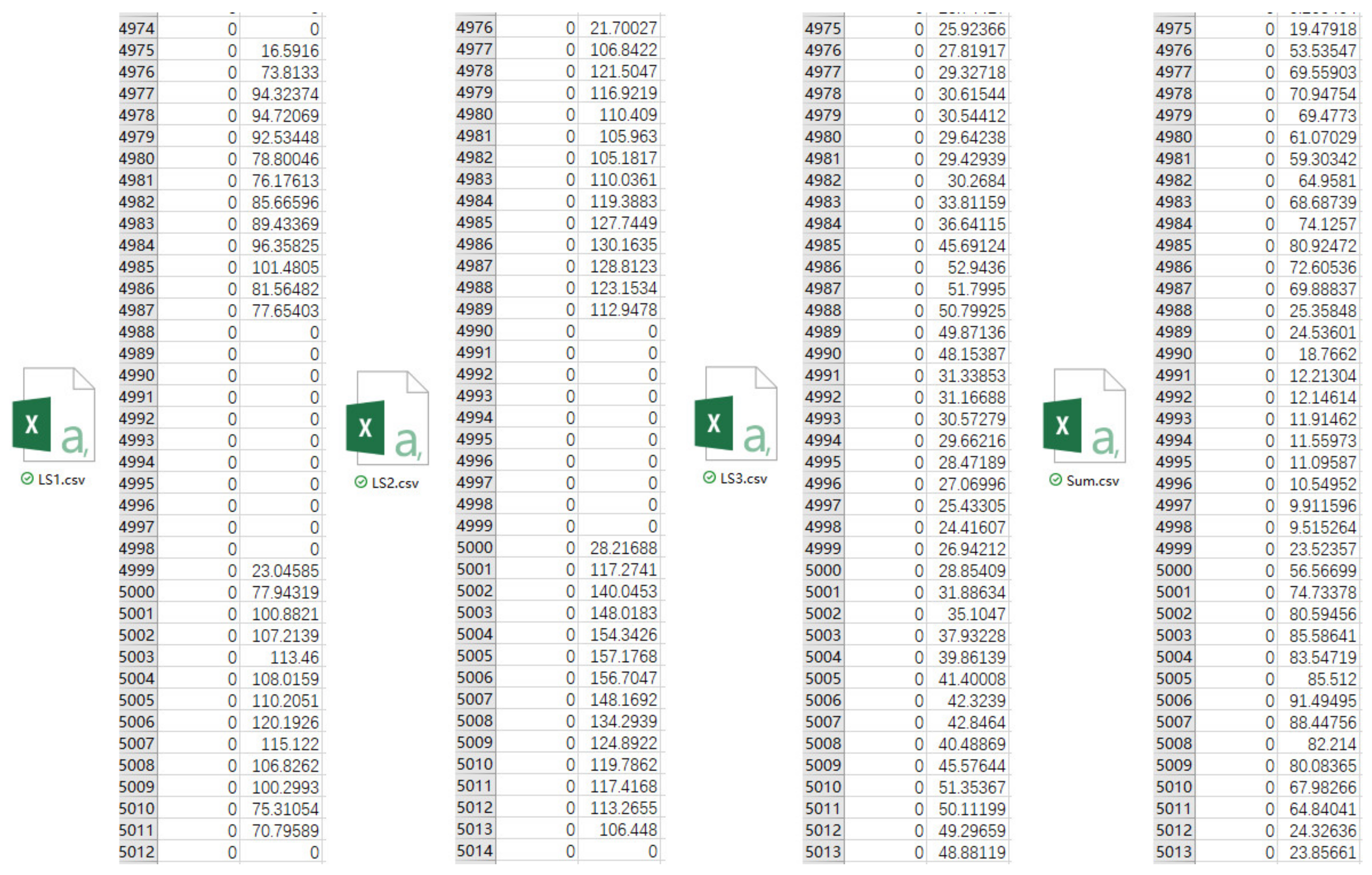
After all variables have been input, the user should click the “Save” button to return to the main UI. Then, the software can start the computation by clicking the “Simulation” button, and a total of four csv files will be generated and opened automatically to show the results (as illustrated by Figure 20). LS1.csv, LS2.csv and LS3.csv are the hourly loads of three types of load source (10 office buildings and shopping malls and 3 hotels, respectively), and Sum.csv is the total hourly cooling and heating loads of the community.

To demonstrate how to apply the software in an actual project, an actual application case is conducted in this paper. We used the fast estimate tool to predict the cooling and heating load of a new community at the planning stage of Shanghai West Hongqiao energy station. This actual project has been analysed by the authors’ team in the previous study [34]. In that paper, we completed the load prediction for community load levelling based on the prototypical model method. Different from the traditional methodology, the predicted loads can be obtained without modelling for the buildings in the community in this study. Up to now, since the energy station has been put into operation for more than one year (only Stage 1 has been completed in total 3 stages), the measurement data of annual cooling and heating energy in the metering system of the energy station can be utilized to show the difference between the predicted results made at the planning stage and the actual values in operation.

The planning information of the district is as follows: the settings of input parameters are listed in

Table 7. Settings of other parameters for load prediction.

Building	Shape Factor [m−1]	ARST	Floor Height [m]	ARWW	Number of Floors
Office	0.200	0.268	4	0.5	12
Shopping mall	0.151	0.299	4.5	0.5	4
Hotel	0.193	0.282	4	0.5	24

; and the planning building areas and the scenario settings of the three types of buildings in this district are listed in

Table 8. Building areas and scenario settings of 3 types of buildings.

Building	Building Area [m2]	Probability
		Scenario 1	Scenario 2	Scenario 3
Office	142,265	0.3	0.4	0.3
Shopping mall	11,368	0.4	0.4	0.2
Hotel	98,106	0.3	0.5	0.2
Total	251,739	-	-	-

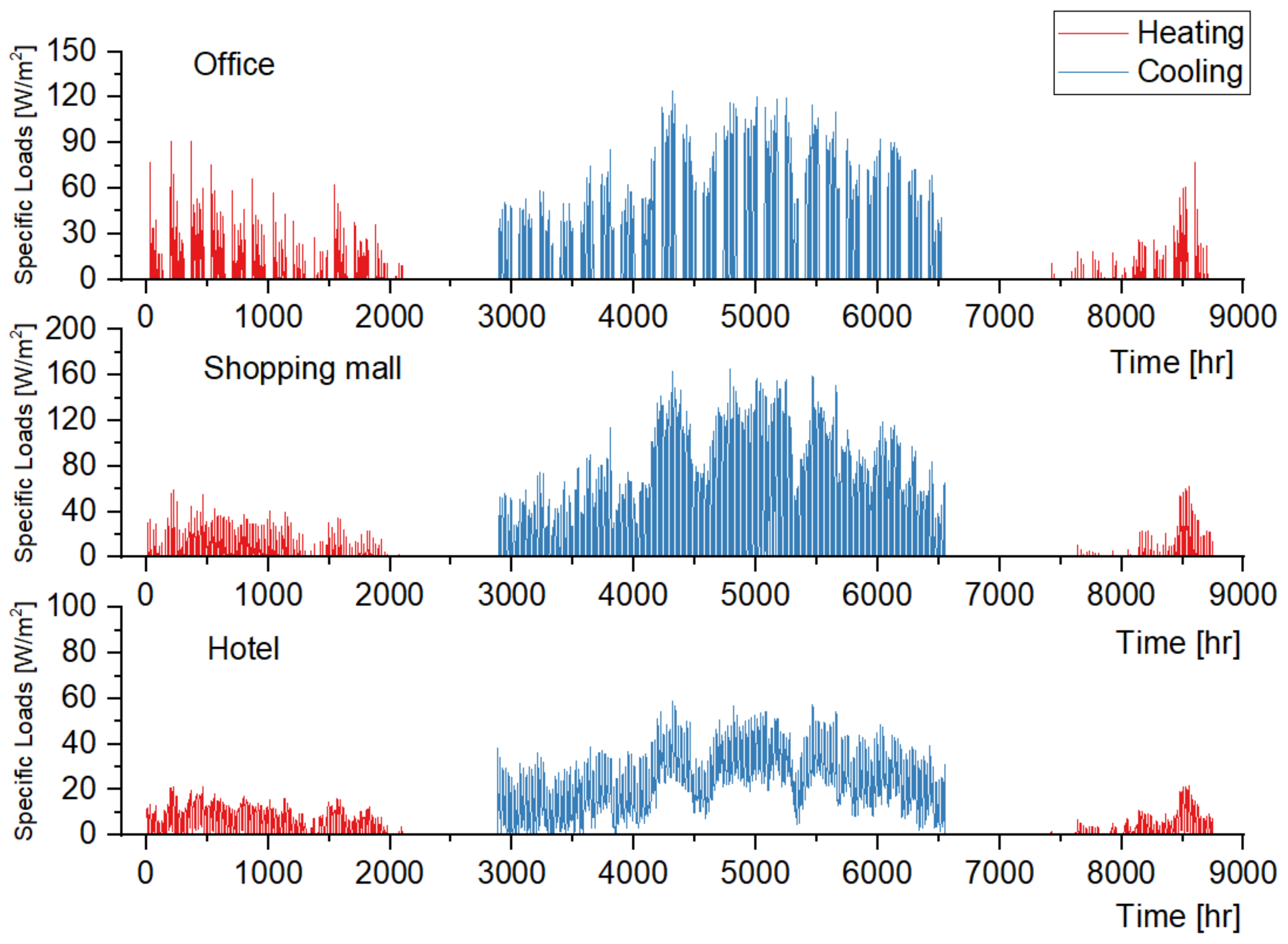
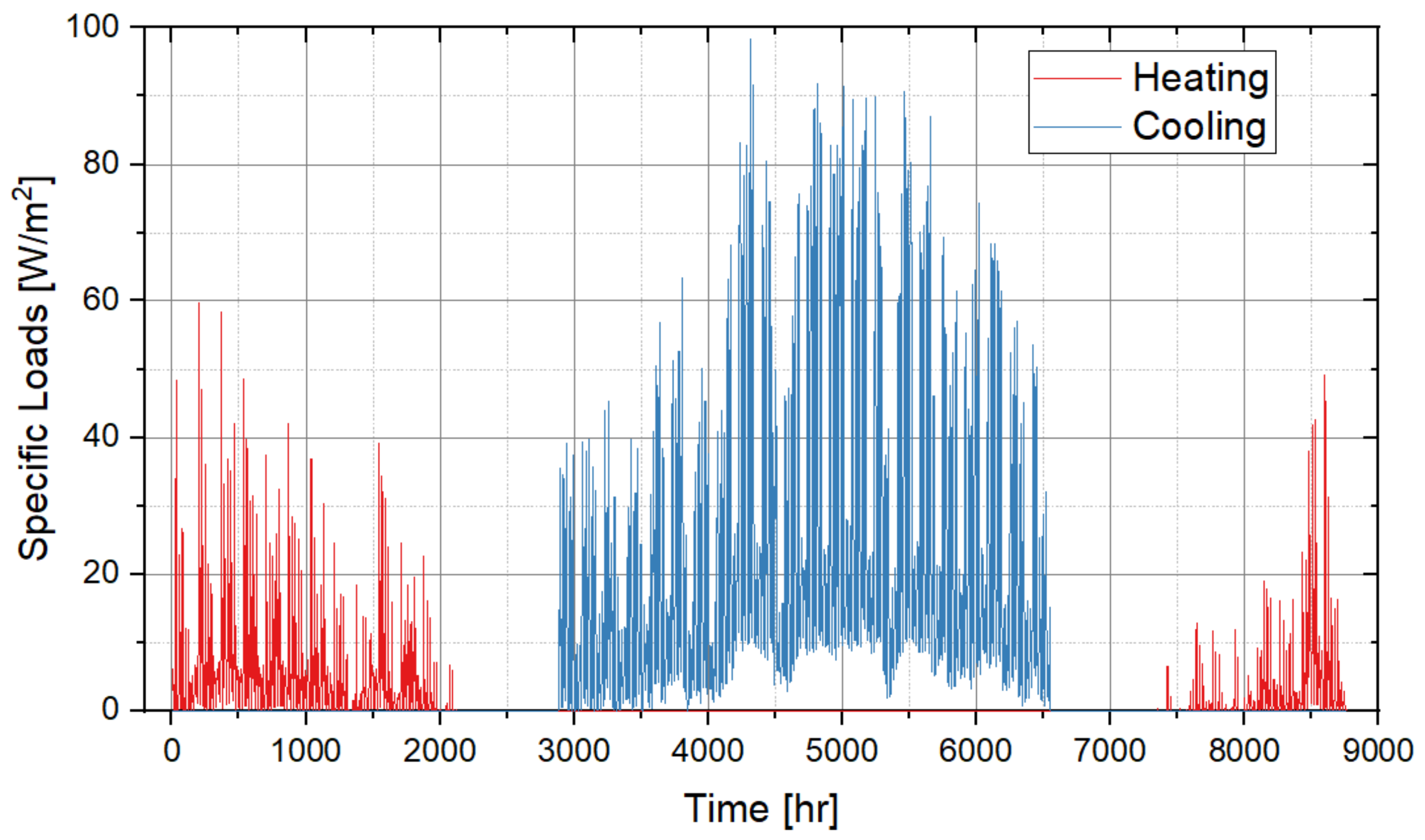
. The input information of this actual case in the software UI has been already shown in Figure 18 and Figure 19. The three types of load source in Figure 18 are consistent with the three building types in Table 7. As a display of the prediction result, the predicted values of hourly specific cooling and heating loads of these three buildings for the whole year are shown in Figure 21. The hourly cooling and heating load of the district can be obtained by multiplying the specific loads per unit floor area of the three buildings with the building area and adding them together. The result is as illustrated by Figure 22.

By adding 8760 hourly cooling and heating loads of the whole year together, the annual cooling and heating energy that the energy station supplies to the district would be obtained. According to the energy audit data of the past year, we can determine the actual cooling and heating energy generated by the energy station in 2020. In

Table 9. Comparison between predicted and actual annual cooling/heating energy.

Annual Specific Energy	Cooling Season [kWh/m2]	Heating Season [kWh/m2]
Actual value	69.55	13.86
Predicted value by detailed modelling	85.08	16.17
RE	22.32%	16.69%
Predicted value by fast estimate tool	82.36	14.48
RE	18.42%	4.50%

, the actual values of annual cooling and heating energy and the predicted values calculated by the fast estimate tool and the detailed modelling method are compared with each other. The result shows that this fast load estimate tool can provide the same level of prediction accuracy as traditional simulation methods. To a certain extent, the prediction result obtained by the fast estimate tool is smaller and better than the simulation result of detailed modelling, since the design load is generally much greater than the actual load. In addition, the index used in Section 3, “ratio of the hours with effective prediction”, which reflects the prediction accuracy on the hourly scale, is also computed based on the predicted loads of the planning district in this section. Since the measurement data of hourly loads is unavailable, this paper only compares the predicted values by detailed modelling (selected as the reference values) and the values by fast estimate tool (as listed in

Table 10. “Ratio of the hours with effective prediction” on the scale of district prediction.

Cooling/Heating	Cooling Season	Heating Season
Number of the hours with nonzero load	3635	3200
Number of the hours with RE >15%	2	1
“Ratio of the hours with effective prediction”	99.97%	99.95%

). The result further indicates that there are not any significant differences between the prediction accuracy of the fast estimate tool and the traditional modelling method on the one hand, and it confirms the conclusion drawn in the previous section on the other hand: the prediction error at the hours with small absolute values of predicted loads will not cause a big bias for district energy planning.

5. Conclusions

The present research introduces a new method for fast cooling/heating load prediction of a district energy system at the planning stage. Based on this new method, a practical tool has been developed in this paper. Firstly, we established a presimulated building model database to provide sufficient data for the machine learning-based load prediction method. Then, we developed the fast estimate tool for load prediction based on the KNN algorithm and the presimulated database. Next, we conducted a test that contains 45 virtual test cases to compare the prediction performance of this tool and detailed modelling. Finally, we also introduced a case of a real energy station to demonstrate the application of this tool in actual project. As the main achievement of this study, the fast estimate tool for load prediction developed in this study has been verified to be able to provide the same level of prediction accuracy as traditional simulation methods, while it is easy to be used by nonprofessionals and saves a lot time for modelling.

However, there are some shortcomings to this study that can be improved in further research. The improvement work could mainly be carried out in following two respects:

(1) A presimulated database with more input parameters.

Considering the actual situation in the planning stage, the thermal property of the envelope and the indoor condition are not available for users to change in the settings, but they are only involved in the selection of different design scenarios. This may be good just for the situation in this study, but more variable model parameters for load prediction can make the new method also applicable for work in the stage of detailed scheme design. For example, the U-values of the exterior wall/window/roof, the SHGC of the exterior window, the density of lighting power, plug equipment power and occupancy can all be set as variable parameters for users to input, and thereby this fast estimate tool can be used to analyse a more detailed design scheme.

To reveal the deviation caused by ignoring the differences between the envelope parameters in different design scenarios, we used the fast estimate tool to carry out an additional simulation test based on the results of the case study in Chapter 4. The main steps of the test are as follows:

Step 1. Find the original EnergyPlus models that were used to output the predicted annual cooling/heating energy “by detailed modelling” and check the settings of the envelope parameters. Their values should be set according to Table 3.

Step 2. Assume that there would be two other virtual communities; the types, areas and indoor conditions of the buildings in these communities are the same as the real community in the case study, but only the envelopes are different. For one virtual community (VC 1), the buildings are all well-insulated; and for another (VC 2), the envelopes are very light. Therefore, the envelope parameters of the EnergyPlus models should be adjusted to the values in

Table 11. Envelope parameters of the buildings in two virtual communities.

Item	Unit	VC 1	VC 2
(1) Heat transfer coefficient of exterior wall	W/(m2·K)	0.4	1.0
(2) Heat transfer coefficient of roof	W/(m2·K)	0.3	0.75
(3) Heat transfer coefficient of exterior window	W/(m2·K)	1.8	3.0
(4) SHGC of exterior window (northward)		0.25	0.45
(5) SHGC of exterior window (others)		0.25	0.45

to simulate the annual cooling/heating load of these two virtual communities.

Step 3. Compare the predicted values between the original models and VC 1 or 2 (

Table 12. Comparison between the predicted values of original models and VC 1 or 2.

Predicted Values by Fast Estimate Tool	Specific Cooling Energy [kWh/m2]	Specific Heating Energy [kWh/m2]
Original models	82.36	14.48
VC 1 (well-insulated)	81.03	12.87
RE	−1.61%	−11.12%
VC 2 (poorly insulated)	87.51	18.83
RE	6.26%	30.06%

). It indicates that the relative errors of −1.61%~6.26% (annual specific cooling energy) and −11.12%~30.06% (annual specific heating energy) caused by ignoring the differences in the thermal properties of building envelope will be probably introduced to the results when using this tool to analyse a community in Shanghai. On one hand, this deviation can be sometimes accepted at the planning stage of a district energy system, even though the RE of the specific heating energy is relatively high, but the absolute value of the error is still acceptable. On the other hand, it also shows that making more input parameters editable in the estimate tool is a valuable research direction, which will further improve the computation accuracy of the tool.

An upgraded estimate tool with more input parameters means a larger presimulated database. The approach to establish such a larger database is similar to what is introduced in this paper. However, the main difficulty is too much computation. If all the parameters listed above are considered, the dimension number of the database will be 11. Supposing that there are five levels on each dimension and also three types of building, the number of models in the database will be more than 1.46 × 10⁸ (3 × 5¹¹). The establishment and storage of such a large database is extremely inconvenient. The method of sampling or clustering may be needed to reduce the size of the database.

(2) More applications in actual conditions.

The new load prediction tool has been only applied in one actual project in this paper. Even in this application case, we can still find that the predicted value of load in the design phase is often larger than the real situation. In the goal of this paper, the benchmarking object of the fast load prediction tool is only the simulation method based on BPS models. Therefore, the gap between predicted and actual values would be the next problem to be solve. By applying this tool in more actual energy stations with measurement data, the key factors that affect the actual cooling and heating load and make it deviate from the predicted result may be found. This work can further improve the practical application value of this new load prediction tool.

References

1. Wu, X.; Wang, Y.; Song, C.; Tian, C.; Qin, X. Thinking of district energy system based on HVAC professional perspective—Concept, planning and design. HV AC 2017, 49, 2–14. [Google Scholar]
2. UNEP (United Nations Environment Program). District Energy in Cities: Unlocking the Potential of Energy Efficiency and Renewable Energy. 2016. Available online: https://www.unep.org/resources/report/district-energy-cities-unlocking-potential-energy-efficiency-and-renewable-energy (accessed on 1 December 2021).
3. Long, W. Important stage of building energy efficiency: Community energy planning. Heat. Vent. Air Cond. 2008, 3, 31–38. [Google Scholar]
4. Sameti, M.; Haghighat, F. Optimization approaches in district heating and cooling thermal network. Energy Build. 2017, 140, 121–130. [Google Scholar] [CrossRef]
5. Hemmati, R.; Saboori, H. Short-term bulk energy storage system scheduling for load leveling in unit commitment: Modeling, optimization, and sensitivity analysis. J. Adv. Res. 2016, 7, 360–372. [Google Scholar] [CrossRef] [PubMed] [Green Version]
6. Lyu, Y.; Pan, Y.; Liu, H.; Yan, J. Application of cooling and heating load prediction for district energy supply: A case in West Hongqiao 1# energy station. J. Glob. Energy Interconnect. 2021, 4, 197–203. [Google Scholar]
7. Clarke, J.A. Energy Simulation in Building Design, 2nd ed.; Butterworth-Heinemann Elsevier Ltd.: Oxford, UK, 2001. [Google Scholar]
8. Hong, T.; Langevin, J.; Sun, K. Building simulation: Ten challenges. Build. Simul. 2018, 11, 871–898. [Google Scholar] [CrossRef] [Green Version]
9. Zhao, H.; Magoules, F. A review on the prediction of building energy consumption. Renew. Sustain. Energy Rev. 2012, 16, 3586–3592. [Google Scholar] [CrossRef]
10. Han, C.; Duanmu, L.; Shu, H.; Li, X.; Wang, Z. Establishment of district building models for cooling load prediction. Build. Energy Environ. 2012, 31, 9–11. [Google Scholar]
11. Ourghi, R.; Al-Anzi, A.; Krarti, M. A simplified analysis method to predict the impact of shape on annual energy use for office buildings. Energy Convers. Manag. 2007, 48, 300–305. [Google Scholar] [CrossRef]
12. Nihar, K.; Bhatia, A.; Garg, V. Optimal control of operable windows for mixed mode building simulation in EnergyPlus. IOP Conf. Ser. Earth Environ. Sci. 2019, 238, 012052. [Google Scholar] [CrossRef]
13. Zhu, L.; Zhang, J.; Wang, F.; Sun, Y.; Tian, W.; Zhu, C. Prediction and characteristics analysis of building heating and cooling loads at planning phase. J. Cent. South Univ. Sci. Technol. 2020, 51, 2969–2977. [Google Scholar]
14. Lim, H.; Zhai, Z. Influences of energy data on Bayesian calibration of building energy model. Appl. Energy 2018, 231, 686–698. [Google Scholar] [CrossRef]
15. Zhu, M.; Pan, Y.; Lyu, Y.; Wang, Q.; Li, Y.; Huang, Z.; Tao, Q. Application review of energy consumption prediction models in building energy efficiency optimization. Build. Sci. 2020, 36, 35–46. [Google Scholar]
16. Korolija, I.; Zhang, Y.; Marjanovic-Halburd, L.; Hanby, V.I. Regression models for predicting UK office building energy consumption from heating and cooling demands. Energy Build. 2013, 59, 214–227. [Google Scholar] [CrossRef]
17. Gayeski, N.T.; Armstrong, P.R.; Norford, L.K. Predictive pre-cooling of thermo-active building systems with low-lift chillers. HVACR Res. 2012, 18, 858–873. [Google Scholar]
18. Sholahudin, S.; Han, H. Simplified dynamic neural network model to predict heating load of a building using Taguchi method. Energy 2016, 115, 1672–1678. [Google Scholar] [CrossRef]
19. Li, Q.; Meng, Q.; Cai, J.; Yoshino, H.; Mochida, A. Applying support vector machine to predict hourly cooling load in the building. Appl. Energy 2009, 86, 2249–2256. [Google Scholar] [CrossRef]
20. Harb, H.; Boyanov, N.; Hernandez, L.; Streblow, R.; Muller, D. Development and validation of grey-box models for forecasting the thermal response of occupied buildings. Energy Build. 2016, 117, 199–207. [Google Scholar] [CrossRef]
21. Chow, T.T.; Fong, K.F.; Chan, A.L.S.; Yau, R.; Au, W.H.; Cheng, V. Energy modelling of district cooling system for new urban development. Energy Build. 2004, 36, 1153–1162. [Google Scholar] [CrossRef]
22. Shimoda, Y.; Yamaguchi, Y.; Okamura, T.; Taniguchi, A.; Yamaguchi, Y. Prediction of greenhouse gas reduction potential in Japanese residential sector by residential energy end-use model. Appl. Energy 2010, 87, 1944–1952. [Google Scholar] [CrossRef]
23. Ren, Z.; Paevere, P.; Grozev, G.; Egan, S.; Antieev, J. Assessment of end-use electricity consumption and peak demand by Townsville’s housing stock. Energy Policy 2013, 61, 888–893. [Google Scholar] [CrossRef]
24. Warnken, J.; Bradley, M.; Guilding, C. Exploring methods and practicalities of conducting sector-wide energy consumption accounting in the tourist accommodation industry. Ecol. Econ. 2004, 48, 125–141. [Google Scholar] [CrossRef] [Green Version]
25. Jiang, X.; Long, W.; Li, M. Hourly cooling load analysis and prediction in a district cooling system. J. Cent. South Univ. 2010, 1, 357–363. [Google Scholar]
26. Wan, K.; Li, H.; Liu, D.; Lam, J. Future trends of building heating and cooling loads and energy consumption in different climates. Build. Environ. 2011, 46, 223–234. [Google Scholar] [CrossRef]
27. Shamshirband, S.; Petkovic, D.; Enayatifar, R.; Abdullah, A.H.; Markovic, D.; Lee, M.; Ahmad, R. Heat load prediction in district heating systems with adaptive neuro-fuzzy method. Renew. Sustain. Energy Rev. 2015, 48, 760–767. [Google Scholar] [CrossRef]
28. Al-Shammari, E.T.; Keivani, A.; Shamshirband, S.; Mostafaeipour, A.; Yee, P.L.; Petkovic, D.; Ch, S. Prediction of heat load in district heating systems by Support Vector Machine with Firefly searching algorithm. Energy 2016, 95, 266–273. [Google Scholar] [CrossRef]
29. Ferracuti, F.; Fonti, A.; Ciabattoni, L.; Pizzuti, S.; Arteconi, A.; Helsen, L.; Comodi, G. Data-driven models for short-term thermal behaviour prediction in real buildings. Appl. Energy 2017, 204, 1375–1387. [Google Scholar] [CrossRef]
30. Reinhart, C.F.; Davila, C.C. Urban building energy modeling—A review of a nascent field. Build. Environ. 2016, 97, 196–202. [Google Scholar] [CrossRef]
31. Ferrando, M.; Causone, F.; Hong, T.; Chen, Y. Urban building energy modeling (UBEM) tools: A state-of-the-art review of bottom-up physics-based approaches. Sustain. Cities Soc. 2020, 62, 102408. [Google Scholar] [CrossRef]
32. Abbasabadi, N.; Ashayeri, M.; Azari, R.; Stephens, B.; Heidarinejad, M. An integrated data-driven framework for urban energy use modeling (UEUM). Appl. Energy 2019, 253, 113550. [Google Scholar] [CrossRef]
33. Deng, Z.; Chen, Y.; Yang, J.; Chen, Z. Archetype identification and urban building energy modeling for city-scale buildings based on GIS datasets. Build. Simul. 2022, 15, 1547–1559. [Google Scholar] [CrossRef]
34. Hong, T.; Chen, Y.; Luo, X.; Luo, N.; Lee, S.H. Ten questions on urban building energy modeling. Build. Environ. 2020, 168, 106508. [Google Scholar] [CrossRef] [Green Version]
35. Xu, L.; Pan, Y.; Lin, M.; Huang, Z. Community load leveling for energy configuration optimization: Methodology and a case study. Sustain. Cities Soc. 2017, 35, 94–106. [Google Scholar] [CrossRef]
36. GB 50189:2015; Design Standard for Energy Efficiency of Public Buildings. China Architecture & Building Press: Beijing, China, 2015.
37. American Society of Heating, Refrigerating and Air-Conditioning Engineers (ASHRAE). ASHRAE Guideline 14-2014: Measurement of Energy, Demand and Water Savings; American Society of Heating, Refrigerating and Air-Conditioning Engineers: Atlanta, GA, USA, 2014. [Google Scholar]
Figure 1. Flow chart of the methodology.
Buildings 12 01671 g001
Figure 2. Models of the actual building and in database.
Buildings 12 01671 g002
Figure 3. Indoor design temperature in summer.
Buildings 12 01671 g003
Figure 4. Indoor design temperature in winter.
Buildings 12 01671 g004
Figure 5. Schedule of lighting power density.
Buildings 12 01671 g005
Figure 6. Schedule of plug equipment power density.
Buildings 12 01671 g006
Figure 7. Schedule of occupant density.
Buildings 12 01671 g007
Figure 8. All arrangements of variable model parameters.
Buildings 12 01671 g008
Figure 9. Prototypical building model in DesignBuilder.
Buildings 12 01671 g009
Figure 10. Structure of the presimulated model database.
Buildings 12 01671 g010
Figure 11. Principle of KNN algorithm.
Buildings 12 01671 g011
Figure 12. Building models of 45 test cases.
Buildings 12 01671 g012
Figure 13. Original results of Cases 1~15.
Buildings 12 01671 g013
Figure 14. Original results of Cases 16~30.
Buildings 12 01671 g014
Figure 15. Original results of Cases 31~45.
Buildings 12 01671 g015
Figure 16. “Ratio of the hours with effective prediction” of 45 test cases.
Buildings 12 01671 g016
Figure 17. Other indices to evaluate the prediction accuracy.
Buildings 12 01671 g017
Figure 18. Main UI of the fast estimate tool.
Buildings 12 01671 g018
Figure 19. UI of the detail parameter settings.
Buildings 12 01671 g019
Figure 20. Computation result files.
Buildings 12 01671 g020
Figure 21. Predicted hourly specific cooling and heating loads of three types of buildings.
Buildings 12 01671 g021
Figure 22. Predicted hourly total cooling and heating loads of the district energy system.
Buildings 12 01671 g022