A Comprehensive Study on Integrating Clustering with Regression for Short-Term Forecasting of Building Energy Consumption: Case Study of a Green Building

Abstract

Integrating clustering with regression has gained great popularity due to its excellent performance for building energy prediction tasks. However, there is a lack of studies on finding suitable regression models for integrating clustering and the combination of clustering and regression models that can achieve the best performance. Moreover, there is also a lack of studies on the optimal cluster number in the task of short-term forecasting of building energy consumption. In this paper, a comprehensive study is conducted on the integration of clustering and regression, which includes three types of clustering algorithms (K-means, K-medians, and Hierarchical clustering) and four types of representative regression models (Least Absolute Shrinkage and Selection Operator (LASSO), Support Vector Regression (SVR), Artificial Neural Network (ANN), and extreme gradient boosting (XGBoost)). A novel performance evaluation index (PI) dedicated to comparing the performance of two prediction models is proposed, which can comprehensively consider different performance indexes. A larger PI means a larger performance improvement. The results indicate that by integrating clustering, the largest PI for SVR, LASSO, XGBoost, and ANN is 2.41, 1.97, 1.57, and 1.12, respectively. On the other hand, the performance of regression models integrated with clustering algorithms from high to low is XGBoost, SVR, ANN, and LASSO. The results also show that the optimal cluster number determined by clustering evaluation metrics may not be the optimal number for the ensemble model (integration of clustering and regression model).

1. Introduction

The building sector is recognized as a major consumer of energy worldwide. According to the United Nations Environment Program (UNEP), the building sector accounts for 40% of global energy [1] and contributes to one-third of the global carbon emissions [2,3]. The energy consumed by buildings in the operation phase accounts for 80% to 90% of the entire life cycle [4]. Therefore, many efforts have been made to decrease the energy consumption of buildings, especially in its operation phase. For example, many buildings are retrofitted to save energy with many energy-saving technologies, such as photovoltaic technology, solar thermal technology, ground source pump technology, and automatic sunshade [5]. However, more operation systems mean they are more likely to cause operation defaults. According to some reports [6,7], the energy saved after building renovation remains below design expectations. The study of this paper in fact arises from a requirement from a green building in Shenzhen, to detect abnormal energy consumption in real-time. More specifically, the total energy consumption in the coming hour needs to be predicted. After the measured data are obtained, the manager can compare the predicted data with the measured data. If there is a great difference between them, the manager can respond immediately to detect faults.

In general, prediction models can be divided into physical and data-driven models [8]. Physical models forecast energy consumption based on thermal dynamics and the energy behavior of buildings. Many software products have been developed based on physical models, including EnergyPlus, DOE-2, TRNSYS, and eQUEST [9]. However, physical models present some deficiencies such as professional knowledge requirements, and the high costs of data collection and computation [10]. For green buildings with many energy-saving technologies, many systems are involved. This means that, in addition to the physical models of buildings, the models of systems are also needed, which can further increase workload and difficulties.

Compared with physical models, little information about physical buildings and systems is required for data-driven models. The models themselves can discover potentially useful (sometimes previously unknown) relationships with efficient computation. Therefore, high prediction accuracy can be achieved without much domain knowledge. In addition, more and more building operational data can be obtained from the Building Automation System (BAS). These conditions significantly facilitate the usage of many data-driven models in the building field, such as Least Absolute Shrinkage and Selection Operator (LASSO) [11], Support Vector Regression (SVR) [12,13], Artificial Neural Network (ANN) [14,15], and extreme gradient boosting (XGBoost) [16].

With the rapid development of prediction technology, one of the ensemble machine learning technologies, the integration of clustering and regression, has gained great popularity in the building field because of its excellent performance. In the study of Wang et al. [11], K-means++ was used for data clustering, and for each cluster, LASSO and Long Short-Term Memory (LSTM) were used to capture the linear and nonlinear relationship within the data, respectively. The results indicate that the integration of clustering and regression can predict short-term solar intensity with higher precision. In the study of Yang et al. [17], k-Shape clustering was combined with SVR models to improve the building energy forecasting accuracy of ten institutional buildings. The results revealed that the forecasting accuracy of the SVR model is significantly improved by utilizing the results of the proposed clustering method. In the study of Karijadi et al. [18], a fuzzy C-means clustering approach was processed before SVR to predict building electricity load. The experimental results demonstrated that this implementation could improve SVR prediction accuracy. In the study of Li et al. [19], the same combination (fuzzy C-means clustering algorithms and SVR) was used to predict cooling load. It was also found that the performance of the ensemble model is better than the single SVR model. In the study of Zhou [20], an ensemble model that combines an ANN model based on the K-means cluster algorithm was proposed to predict system operation energy consumption. It could be found that the ensembled ANN model has a higher prediction accuracy than the original ANN model. In the study of Zheng and Wu [21], the K-means clustering algorithm was ensembled with an extreme gradient boosting (XGBoost) model for short-term wind power forecasting. It was shown that the proposed model produces a higher forecasting accuracy than the original XGBoost.

When integrating clustering and regression models, the cluster number is an important parameter to be determined. Going through different cluster numbers might be quite time-consuming, because an individual model is needed for each cluster, and there are normally many parameters to be optimized in each model. In recent studies, instead of going through all possible cluster numbers, clustering evaluation metrics was used directly to determine the optimal cluster number. In the study of Karijadi et al. [18], a fuzzy C-means clustering approach was processed before SVR to predict building electricity load. The optimal cluster number was determined by the Modified Partition Coefficient (MPC) index. The experimental results demonstrated that this implementation could improve SVR prediction accuracy. In the study of Luo [22], K-means clustering was ensembled with ANN to forecast the building cooling demand 24 h ahead where the cluster number was determined by the Davies–Bouldin index. The results indicated that the ensembled model had a 4.2% and 3.1% improvement compared to the original ANN model. In the study of Chen et al. [23], the improved K-means clustering method was ensembled with XGBoost for power saving potential prediction where the optimal cluster number was also determined by the Davies–Bouldin Index. In the study of Wang [24], wind turbine clustering was combined with CFD pre-calculated flow fields for wind power forecasting. The Calinski–Harabaz index (CHI) was used to find the optimal number of clusters. The results indicated that the clustering approach can decrease the annual forecasting RMSE of the whole wind farm by up to 5.2%.

In summary, current studies have shown that the integration of clustering and regression can predict more accurately than the original regression model [25]. The fundamentals of performance improvement can be explained as follows. A certain prediction task normally includes many patterns. Taking building energy consumption as an example, there are different patterns, such as different months with different weather conditions, working days and nonworking days, and working hours and nonworking hours. The use of clustering analysis can automatically find these patterns or even some underlying patterns that were previously unknown and separate them into different groups. Then, dedicated regression models are used for different patterns with homogeneous datasets. This can technically improve the prediction accuracy. However, some questions have not been answered properly in previous studies.

• First, there are many types of regression models. What types of regression models are suited for integrating clustering?
• Second, previous studies have demonstrated that the ensemble model can improve the prediction performance of the regression using the cluster number determined by clustering evaluation metrics. However, this number is only the optimal number for the clustering algorithm. Is it also the optimal number for the prediction performance of ensemble models?
• Third, which ensemble model has the best performance for short-term forecasting of building energy consumption?

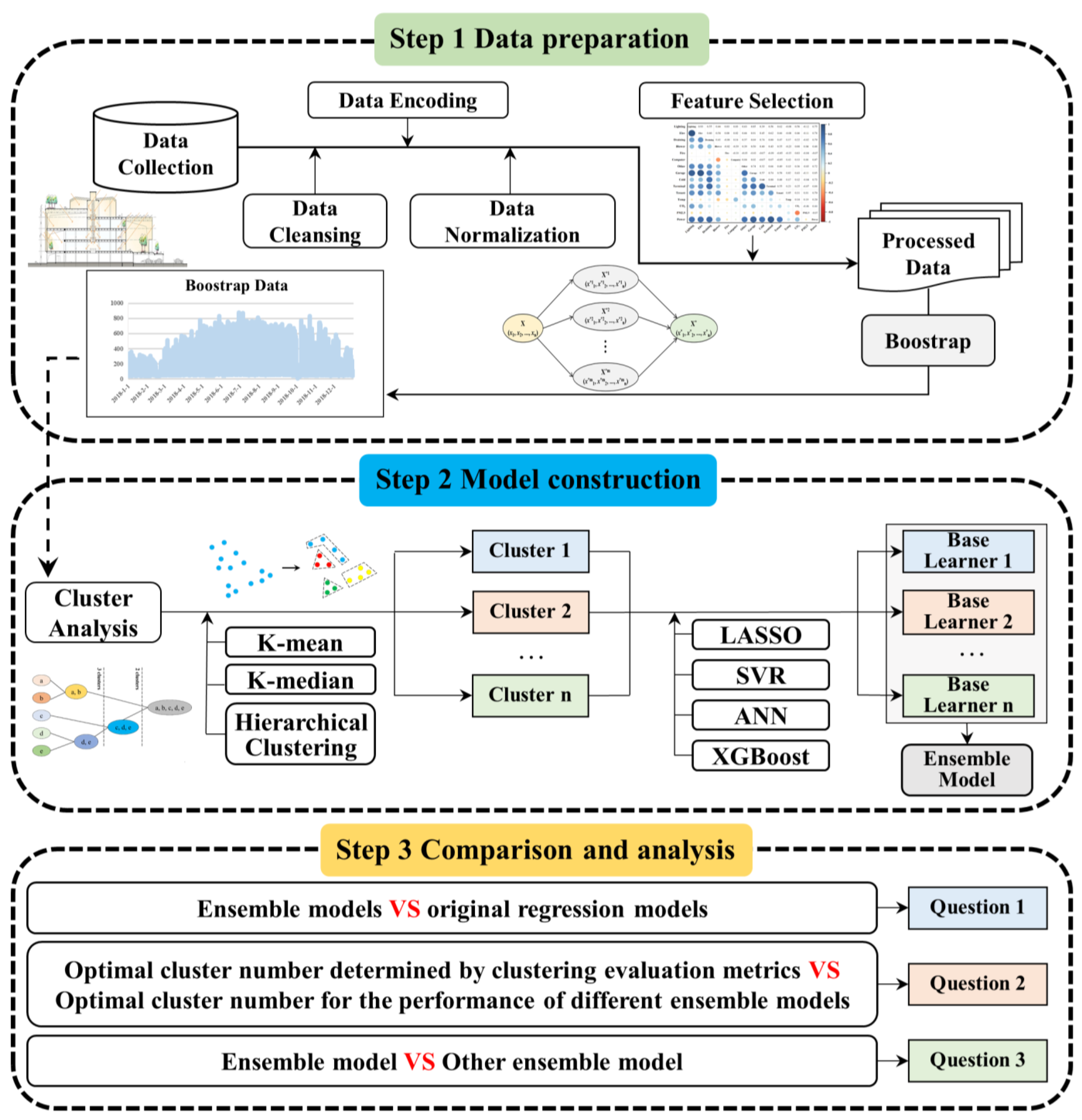
In this study, based on a practical requirement in a project (with the object of a real green office building in Shenzhen, China), a comprehensive study is conducted to systematically study the integration of clustering and regression and answer the above questions. More specifically, this study considers three clustering algorithms (K-means, K-medians, and Hierarchical clustering) and four representative regression models (LASSO, SVR, ANN, and XGBoost) to study the performance improvement of various integrations of clustering and regression models. A novel performance evaluation index dedicated to comparing the performance of two prediction models is also proposed. In addition, different cluster numbers (from 2 to 20 with an increment of 1) are set to find the optimal cluster numbers for different ensemble models, and these numbers are compared with the optimal cluster numbers determined by clustering evaluation metrics.

This paper is organized as follows. Section 2 presents the research outline, clustering algorithms and regression models, clustering evaluation metrics, and the proposed performance evaluation index. Section 3 presents the case study of the green building, including data used in detail and model implementation details. In Section 4, the performances of prediction models are compared using the proposed performance evaluation index. The three questions mentioned above are analyzed. Conclusions are drawn in Section 5.

2. Methodology

2.1. Research Outline

Figure 1 presents the general research outline that includes three steps. The first step is data preparation, including data collection, data cleansing, data encoding, data normalization, and feature selection. In the first step, the data expansion technology is used because the data amount may not be sufficient for complicated models (such as ANN and XGBoost). The technologies and methods used in the first step of data preparation are introduced in Section 2.2.

The second step is model construction. In this step, three clustering algorithms (K-means, K-medians, and Hierarchical clustering) and four regression models (LASSO, SVR, ANN, and XGBoost) are integrated, which generates 12 types of ensemble models. There are two reasons for selecting these specific clustering and regression algorithms. First, they are frequently used in the building energy field. Second, they are representative models based on different theories. These clustering algorithms and regression models are introduced in Section 2.3 and Section 2.4, respectively.

In the last step, three comparisons are conducted to answer the three questions mentioned in the Introduction. (1) The performances of ensemble models and the original regression models are compared to find what types of regression models are suited for integrating clustering. Here, a proposed performance evaluation index dedicated to comparing the performance of two prediction models is used, which is introduced in Section 2.5.2. (2) The optimal cluster numbers determined by clustering evaluation metrics and the optimal cluster numbers for the prediction performance of different ensemble models are compared to analyze their relationship. Here, the clustering evaluation metrics used are introduced in Section 2.5.1. (3) The performances of different ensemble models are compared to find the best model for short-term forecasting of building energy consumption. Here, to facilitate the comparison among different ensemble models, the performance of a classical regression model is selected as a baseline. This model is a time series prediction model, Autoregressive Integrated Moving Average (ARIMA) [26], which only uses time sequence data (i.e., historical total energy consumption in this study) as inputs.

2.2. Data Preparation

Three types of data from the building automation system are collected in this study, including time-related data, environmental data, and energy consumption data.

2.2.1. Data Cleansing

In the process of data collection, loss and abnormalities often occur due to signal transmission failures. Therefore, it is necessary to clean the data, namely data cleansing, which is the process of detecting and correcting (or removing) missing or abnormal data and then replacing these data with normal values [27]. In this study, the abnormal data are replaced by the data in the previous time point.

2.2.2. Data Encoding and Normalization

In the energy consumption prediction tasks, many categorical features serving as the inputs need to be encoded into valued variables, such as day type and weather type [8]. In addition, to reduce model prediction errors and improve solution convergence speed and model training efficiency, MinMaxScaler normalization technology [28] is used in this study to normalize the data to distribute between 0 and 1.

2.2.3. Feature Selection

Feature selection is used to obtain useful and representative information from raw data as model inputs. There are two reasons for this implementation. First, feature selection could discard the redundant information contained in the original historical data, which could decrease the risk of over-fitting. Second, feature selection helps to reduce the dimensionality of model inputs, which can reduce the computational load in model development [29,30]. In this study, the Pearson correlation coefficient (PCCs) is used for correlation analysis. The value of PCC is between −1 and 1. A larger absolute value means a stronger linear relationship between two parameters [31].

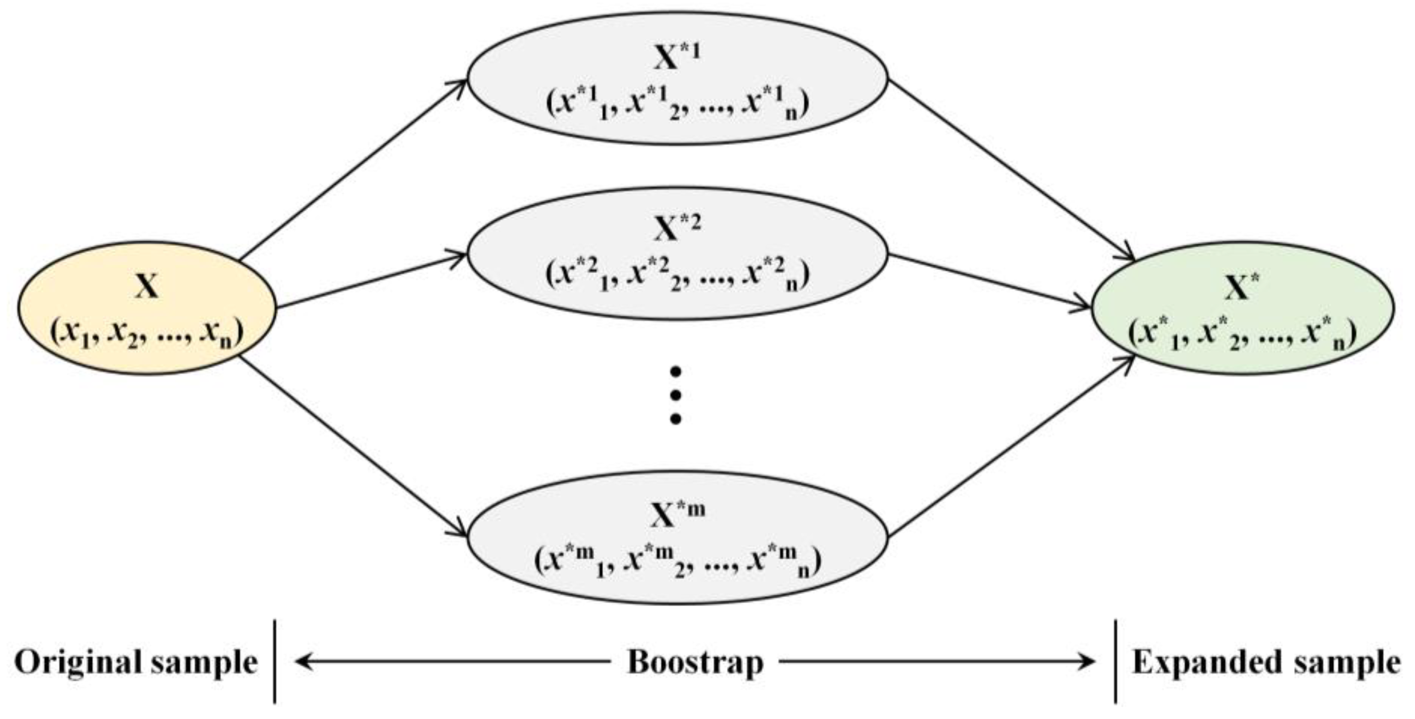
2.2.4. Data Expansion

Bootstrap is a data expansion technology achieved by random resampling of the original data. More specifically, based on the collected data, a certain number of new samples are extracted each time through resampling. It should be noted that data can be repeatedly extracted more than once. Figure 2 shows a schematic of a typical bootstrap process. Each vector (e.g., x₁) in the original dataset (i.e., X) includes all the inputs and outputs. Each bootstrap dataset (e.g., X^*1) is generated by randomly sampling n times from the original dataset (i.e., X). This process is repeated m times until all the bootstrap datasets are generated [32].

2.3. Clustering Algorithms

In this section, three clustering algorithms are briefly introduced, including K-means, K-medians, and Hierarchical clustering.

2.3.1. K-Means Algorithm

The K-means algorithm was proposed by MacQueen [33], which is a widely used clustering algorithm. Classic K-means can divide a set of data into K clusters according to the distance between each dataset and each cluster center, as defined in Equation (1).

$$P^{*}=\arg \min {{\displaystyle \sum }}_{j=1}^K{{\displaystyle \sum }}_{w_i\in p_j}^{n}dist\left({\parallel w_i-c_j\parallel }^2\right)$$

(1)

where $P^{*}$ denotes the best partition; $w_i$ denotes the feature selected (inputs) in the dataset; $c_j$ denotes the cluster center of cluster j. The algorithm first randomly initializes K cluster centers and assigns other data to the nearest cluster. Then, it updates the center of each cluster and iterates the above process. This process terminates until no individual moves to another cluster, or the cluster center does not change anymore [8].

2.3.2. K-Medians Algorithm

The K-medians algorithm is a variation of the K-means algorithm. Therefore, they have the same framework. The main difference between them is the determination of the cluster center. For the K-medians algorithm, the median instead of the average of the individuals in one cluster is recognized as the cluster center [34]. This difference could bring the K-medians algorithm advantages in some scenarios. It is known that the average value can be significantly changed by outliers, while these outliers almost have no impact on the median value. Therefore, the K-medians algorithm might be more effective than the K-means algorithm when outliers are encountered.

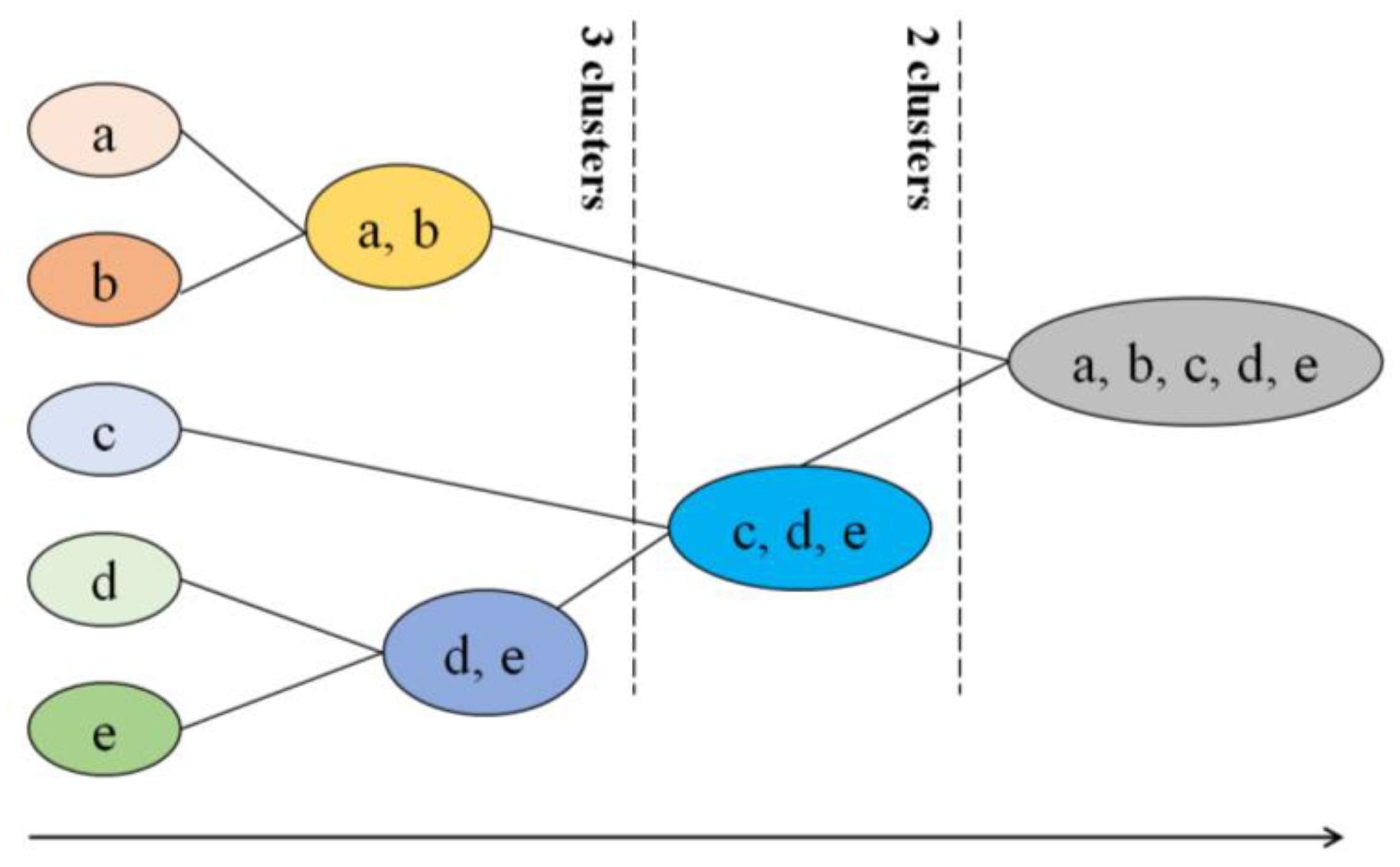
2.3.3. Hierarchical Clustering

In the building energy field, Hierarchical clustering (HC) is normally used to organize datasets into a tree-like hierarchy from bottom to top [35], as illustrated in Figure 3. At the beginning of the algorithm, each data sample (a, b, c, d and e) is treated as a single cluster. To characterize the inter-cluster similarity, the distances among different clusters are computed [35]. Then, the two closest clusters are merged. This merging process iterates until a certain criterion is met, for example, the cluster number is achieved. In this study, the square Euclidean distance is used to calculate the distances among different clusters.

2.4. Regression Models

2.4.1. Least Absolute Shrinkage and Selection Operator

Least Absolute Shrinkage and Selection Operator (LASSO) regression is a modification of linear regression, where the model is penalized for the sum of absolute values of the weights. Thus, the absolute values of weight can be (in general) reduced [36]. In this way, it can effectively simplify the model and reduce the over-fitting problem.

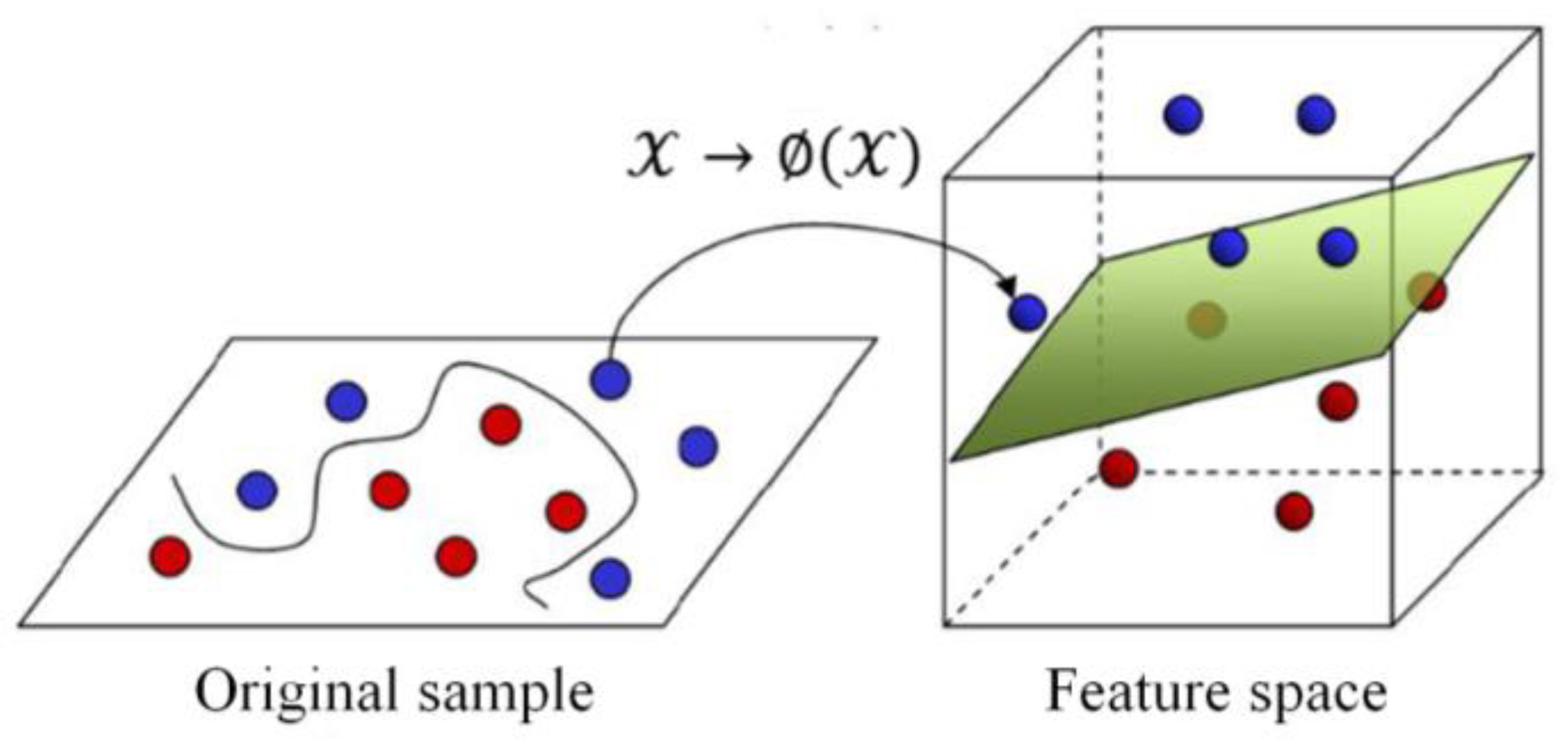
2.4.2. Support Vector Regression

Support Vector Regression (SVR) is a machine learning technique that was proposed by Vapnik et al. [37,38] based on statistical learning theory and the structural risk minimization principle. The basic idea of SVR is to introduce a kernel function, map the input space to a high-dimensional feature space through nonlinear mapping, and carry out linear regression on this feature space. This basic idea can be illustrated in Figure 4.

2.4.3. Artificial Neural Network

The Artificial Neural Network (ANN) is a technique based on a collection of connected units or nodes called artificial neurons. An artificial neuron receives a signal and then processes it, and the output of each neuron is computed by some nonlinear functions. Typically, neurons are aggregated into layers. A typical neural network usually has three layers, i.e., one input layer, one hidden layer, and one output layer. In this study, a fully connected neural network is used.

2.4.4. Extreme Gradient Boosting

Extreme Gradient Boosting (XGBoost) is an improved decision tree algorithm proposed by Chen [39] that uses a gradient boosting framework. Here, boosting is a general term in machine learning where multiple weak learners (e.g., regression trees) are ensembled to create a single strong learner. The gradient boosting (compared with boosting) further enhances the flexibility of the boosting algorithm by constructing the new regression trees to be maximally correlated with the negative of the gradient of the loss function. This helps the convergence of the loss function and allows arbitrary differentiable loss functions to be used in the model building process [40]. Readers can refer to Ref. [41] for more details about regression trees and boosting.

2.5. Performance Evaluation Index

2.5.1. Clustering Evaluation Metrics

In this study, two clustering evaluation metrics are used to calculate the optimal cluster numbers for clustering algorithms, including the Davies–Bouldin index (DBI) and Calinski–Harabaz index (CHI).

The Davies–Bouldin index (DBI) [42] is calculated as the average similarity of each cluster with a cluster most similar to it. A lower DBI means the clusters are better separated, which also means the cluster number is more proper. The similarity of cluster i and j, $R_{ij}$, is described in Equation (2).

$$R_{ij}=\frac{s_i+s_j}{d_{ij}}$$

(2)

where $s_i$ is the intra-cluster dispersion of cluster i, which also means the average distance between each point of cluster i and the center of cluster i; $d_{ij}$ is the distance between the centers of cluster i and cluster j. After finding the most similar cluster for each cluster, the Davies–Bouldin index can be calculated by Equation (3).

$$DB=\frac{1}{k}{{\displaystyle \sum }}_{i=1}^k\underset{i\ne j}{\max }{R}_{ij}$$

(3)

The Calinski–Harabaz index (CHI) [43] (i.e., variance ratio criterion) is described in Equation (4). Here, $B_k/\left(K-1\right)$ is the dispersion of data points (in one cluster) to other clusters. $W_k/\left(N-K\right)$ is the dispersion of these data points to their own cluster. A higher value of CHI means the clusters are dense and well separated, which also means the cluster number is more proper.

$$CH=\frac{B_k}{K-1}/\frac{W_k}{N-K}$$

(4)

$$B_k={{\displaystyle \sum }}_{k=1}^K{n}_k{\parallel c_k-c\parallel }^2$$

(5)

$$W_k={{\displaystyle \sum }}_{k=1}^K{{\displaystyle \sum }}_{i=1}^{n_k}{\parallel d_i-c_k\parallel }^2$$

(6)

where K is the cluster number; N is the total number of data points; $n_k$ is the number of points in cluster k; $c_k$ is the center of cluster k; c is the global center; $d_i$ is each data point.

2.5.2. Prediction Performance Evaluation

In this study, a novel metric called performance improvement (PI) is proposed to comprehensively quantify the performance improvement of the new model compared with the basic model, as shown in Equation (7).

$$PI={{\displaystyle \sum }}_{i=1}^n\frac{1}{n}·\frac{Inde{x}_b}{Inde{x}_p}$$

(7)

where Index refers to the performance index of a prediction model, such as mean absolute error (MAE), mean absolute percent error (MAPE), and root-mean-square error (RMSE). $Inde{x}_b$ is the index of the basic model, while $Inde{x}_p$ is the index of the proposed new model. n is the total number of the performance index.

It can be observed from the equation that PI eliminates the magnitude differences between the evaluation indices by standardization. The comprehensive performance of the proposed new model can be considered better than the basic model when PI is larger than one. A larger PI means a larger performance improvement of the new model compared with the basic model.

In this study, three indexes, MAE, MAPE, and RMSE [44] (as shown in Equations (8)–(10)), are used for the combination of PI. Therefore, PI in this study can be described in Equation (11). It is worth noting that the ensemble model is a couple of many individual models. Therefore, the index of an ensemble model is the weighted average (according to the amount of data in different clusters) of these individual models.

$$MAE=\frac{1}{N}{{\displaystyle \sum }}_{i=1}^N\left|y_i-{\widehat{y}}_i\right|$$

(8)

$$MAPE=\frac{1}{N}{{\displaystyle \sum }}_{i=1}^N\frac{\left|\left(y_i-{\widehat{y}}_i\right)\right|}{y_i}\times 100\%$$

(9)

$$RMSE=\sqrt{\frac{1}{N}{{\displaystyle \sum }}_{i=1}^N{\left(y_i-{\widehat{y}}_i\right)}^2}$$

(10)

where ${\widehat{y}}_i$ is the prediction value of the model; $y_i$ is the measured value; N is the total number of measurements.

$$PI=\frac{1}{3}\times \left(\frac{MA{E}_b}{MA{E}_p}+\frac{MAP{E}_b}{MAP{E}_p}+\frac{RMS{E}_b}{RMS{E}_p}\right)$$

(11)

3. Case Study

As mentioned in the Introduction, this study arises from a requirement from a retrofitted green building in Shenzhen, China. Therefore, the data of this building are directly used for the test.

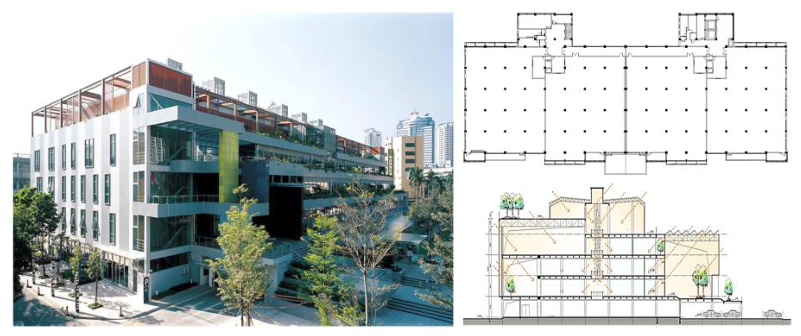
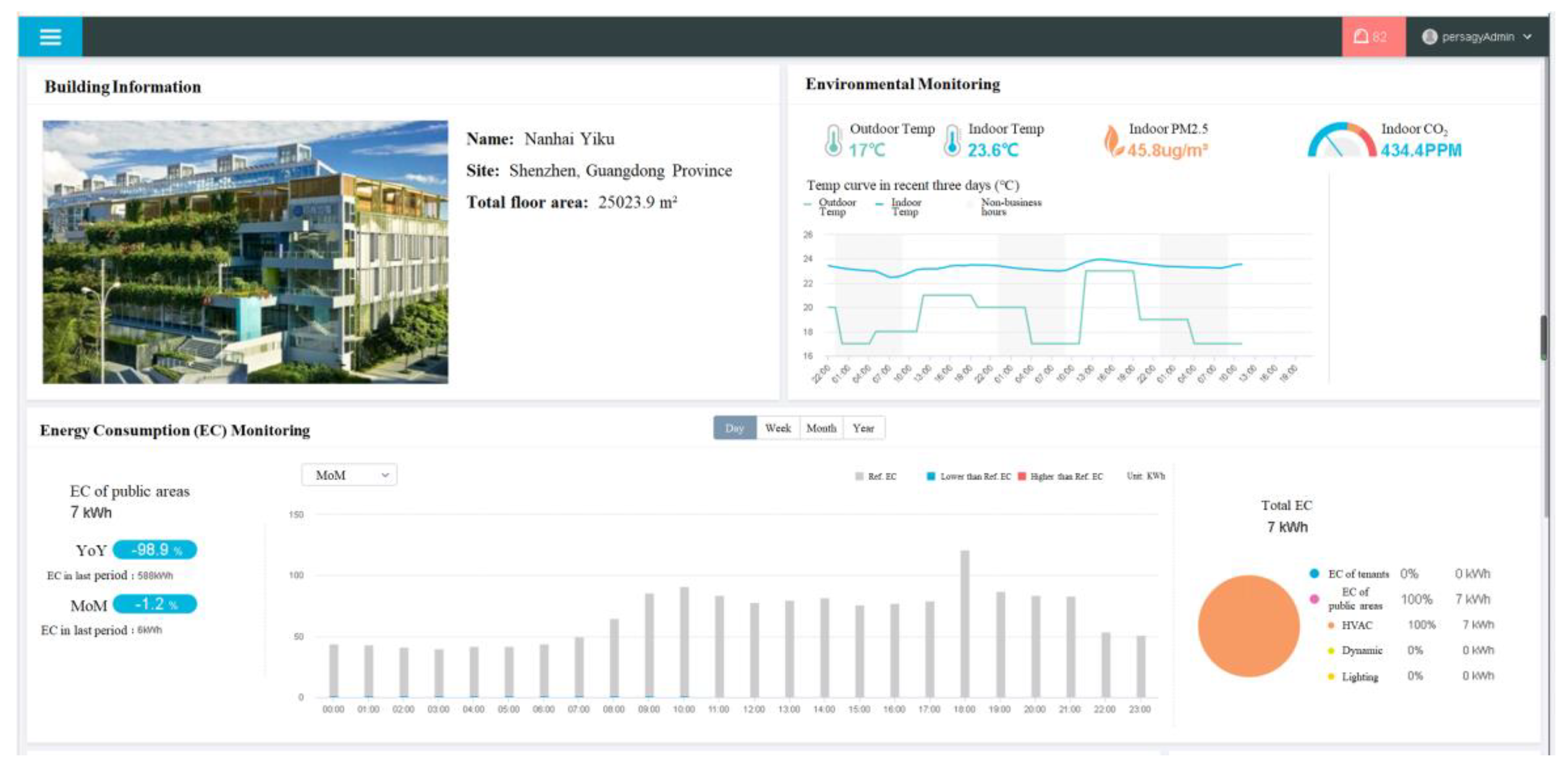
3.1. Building Description

The green building is shown in Figure 5. Some detailed information about this building is summarized in

Table 1. Detailed information of the green building.

Item	Detail
Building type	Office building
Location	Shenzhen, China
Build time	1980s
Floors	5
Height (m)	21.5
Building area (m2)	25,000
Air conditioning area (m2)	16,259

. In this building, the basement is a garage. On the first floor, there are a garage, an administrative office, an equipment room, an archive, and shops. The second to fourth floors are used as technology research and development offices. The fifth floor serves as a multi-purpose hall and an activity room.

The building was retrofitted in 2008 for energy saving. In the process, the architecture was redesigned. Moreover, many energy-saving technologies were used to reduce energy consumption, such as photovoltaic technology, solar thermal technology, ground source pump technology, a rainwater collection system, and artificial wetlands. Therefore, this building is a typical green and energy-saving building and it has won many national green building awards, including the “National Green Building Innovation Award” and “International Housing Association (IHA) Green Architecture Award”.

3.2. Data Preparation

3.2.1. Data Collection

The building is equipped with an intelligent building energy management system (shown in Figure 6) that can monitor real-time operational data. This system collects a large amount of data and presents these data visually. Here, the time interval of data collection is one hour. Moreover, the system can export the collected data in Excel format, which can be accessed easily by Python.

In this study, a total of 18 variables in the current (t) hour are collected as initial inputs (before feature selection) to predict the total energy consumption (one output) in the coming (t + 1) hour, as summarized in

Table 2. Initial inputs and one output of the energy consumption prediction task.

		Parameter	Abbreviation	Unit
Input	Time-related features	Month *	Month
		Day type *	Day type
		Working day type *	Working type
		Hour *	Hour
	Environmental features	Indoor temperature	T	°C
		CO2 concentration	CO2	ppm
		PM2.5 concentration *	PM2.5	μg/m3
	Energy consumption (EC) features	EC of tenants *	Tenant	kW·h
		EC of air conditioning (AC) terminals *	Terminal	kW·h
		EC of cold/heat source of AC systems *	Cold/heat	kW·h
		EC of the public lighting system*	Lighting	kW·h
		EC of the firefighting system	Firefighting	kW·h
		EC of the garage	Garage	kW·h
		EC of elevators	Elevator	kW·h
		EC of draining pumps *	Draining	kW·h
		EC of blowers *	Blower	kW·h
		EC of computer rooms	Computer	kW·h
		Other energy consumption *	Other	kW·h
Output		Total energy consumption	Total	kW·h

* Input selected after the process of feature selection. Other forms of energy consumption include the energy consumption of the emergency lighting system and the fire roller shutter system.

. It can be observed from the table that the initial input variables include time-related features, environmental features, and energy consumption features. Here, the time-related features include month, day type (Sunday, Monday, ..., Saturday), working day type (working day or nonworking day), and hour. The day type and working day type are determined according to the calendar. It should be noted that these two concepts can provide different information because the holiday (nonworking day) could happen on a weekday or a weekend. For energy consumption features, the hourly total energy consumption in the current (t) hour is also known, while it is not included in the inputs. The reason is that the hourly total energy consumption is the sum of each sub-metering that has been included in the inputs.

As mentioned above, the time interval of data collection is one hour. Therefore, for a calendar year (from 1 January 2018 to December 31, 2018), a matrix of 8,760×19 (18 inputs and 1 output) is obtained. There are 24 sets of data missed, which are then filled by the data in the previous time point.

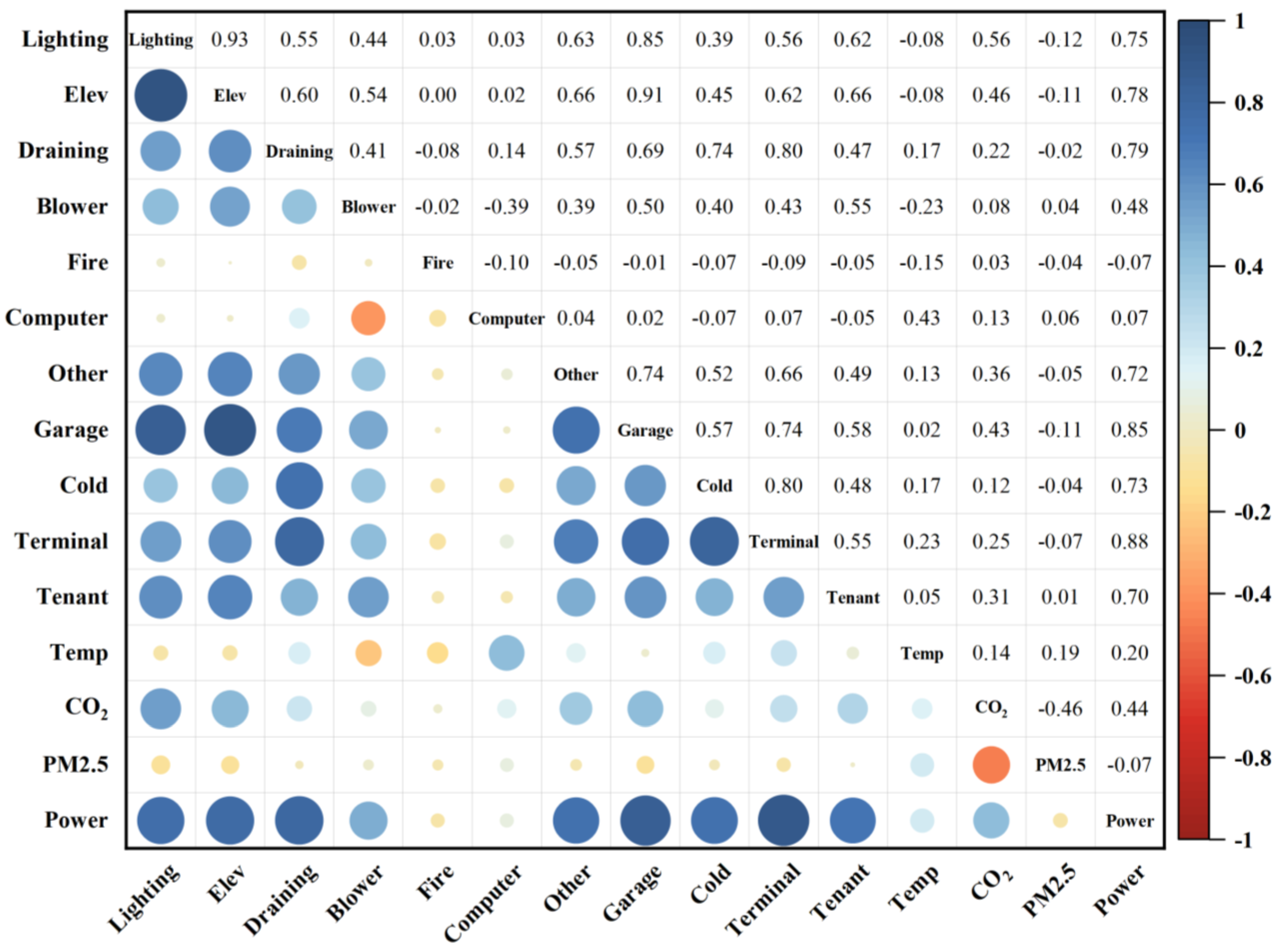
3.2.2. Feature Selection

As mentioned in Section 2.2, the collected data are processed by data cleansing, data encoding, and data normalization. Then, feature selection is conducted, which is introduced as follows. As mentioned in Section 2.2.3, the Pearson correlation coefficient (PCC) is used to quantify the relationship among features and the output. It should be noted that only the environmental features and energy consumption features are implemented by feature selection according to PCC, while the time-related features are not involved. The reason is that PCC can only reflect the linear relationship between variables, while the time-related features normally have a nonlinear relationship with other variables. The results are shown in Figure 7. It can be observed from the figure (the rightmost column) that the PCCs between the total energy consumption (in t + 1 h) and other variables (in t hour) are −0.07 for the energy consumption of the firefighting system, 0.07 for computer room energy consumption, −0.07 for PM2.5, and 0.20 for average indoor air temperature. By comparison, the absolute values of other PCCs are larger than 0.4. Therefore, these four features are discarded in the prediction. Here, the reasons for the weak relationship between these four features and the total energy consumption are analyzed. For the firefighting system, it is in a standing state for the most of time, so its energy consumption is almost constant. Similar to the energy consumption of the firefighting system, the average indoor air temperature also remains stable during the working hours of office buildings. It is interesting to find that the concentration of indoor PM2.5 has a small correlation with the total energy consumption (with a CPP of −0.07), while the concentration of indoor CO₂ has a relatively large correlation with the total energy consumption (with a CPP of 0.44). The reason might be that the indoor CO₂ is partly generated by workers whose number has a strong relationship with energy consumption. By comparison, there is no such relationship for PM2.5. Figure 7 also shows the relationship among different input variables. It can be found that the energy consumption of the lighting system and elevators (with a PCC of 0.93) and the energy consumption of the lighting system and the garage (with a PCC of 0.85) are highly correlated. It is quite reasonable as these three variables are all related to the number of workers. Therefore, only the energy consumption of the lighting system is used, while the other two variables are discarded.

In summary, after feature selection, a total of 12 (i.e., 18 − 6) variables in the current (t) hour are used as inputs to predict the total energy consumption (one output) in the coming hour (t + 1).

3.3. Data Expansion

As mentioned in Section 3.2.1, there are 8760 original datasets in total. In this study, 70% of the datasets (randomly selected) are used as training data and the remaining 30% are used as test data. Then, the bootstrap technology is used to expand the training data. The training data expansion is conducted because the number of datasets in some clusters is not sufficient for fully training the regression model after the process of clustering. To determine a proper expansion time, it is increased gradually. It is found that the prediction performance does not further increase when the expansion time is larger than five. Therefore, five times are determined finally.

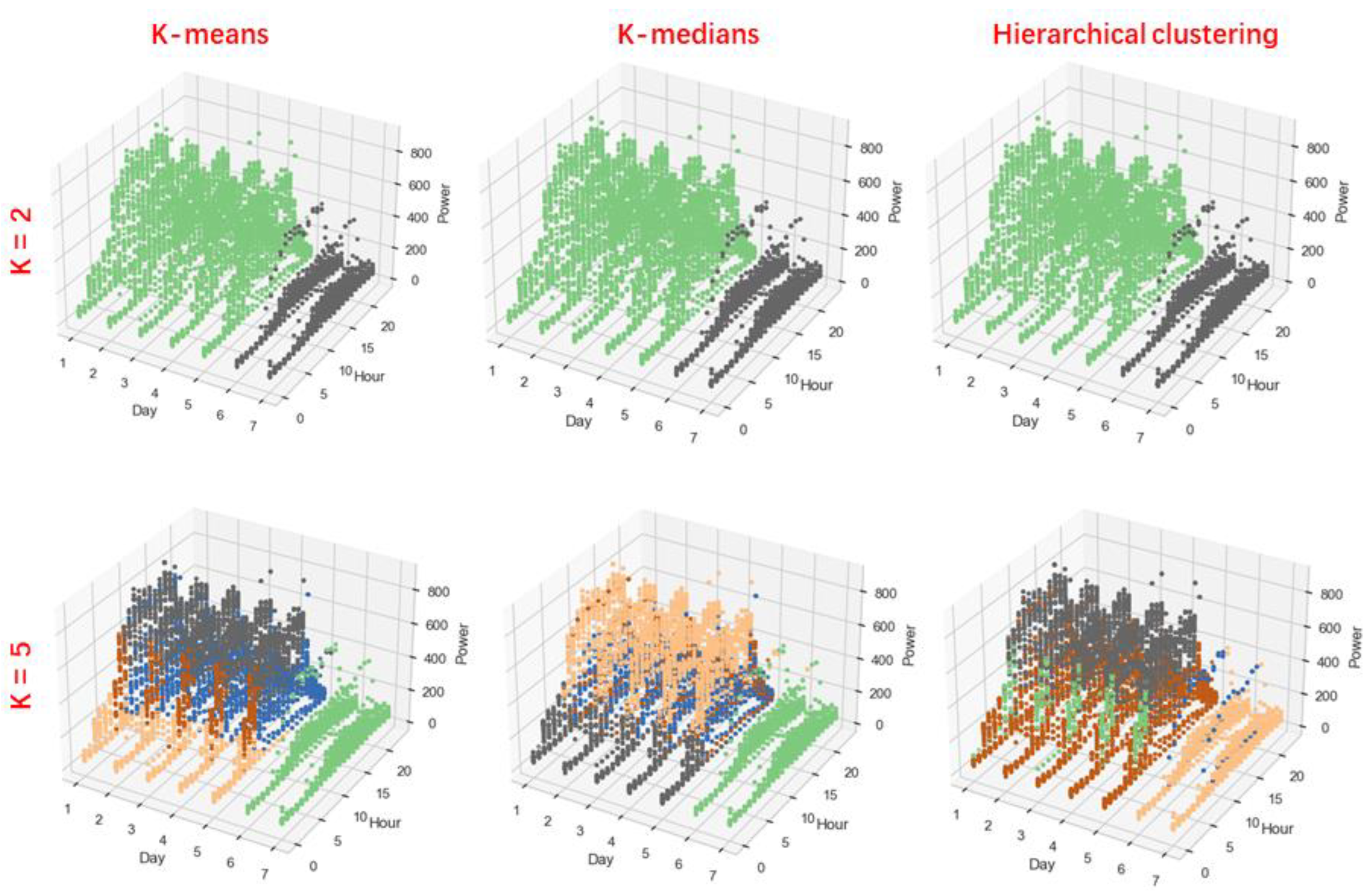
3.4. Cluster Analysis

As mentioned in Section 2.1, the K-means algorithm, K-medians algorithm, and Hierarchical clustering are used for data clustering. Two clustering evaluation metrics (Davies–Bouldin index, DBI, and Calinski–Harabaz index, CHI) are used to calculate the optimal cluster numbers for different clustering algorithms. In addition, different cluster numbers (from 2 to 20 with an increment of 1) are set to find the optimal cluster numbers for different ensemble models, and these numbers are compared with the optimal cluster numbers determined by clustering evaluation metrics.

3.5. Prediction Model Implementation

In this work, three regression models (LASSO, SVR, and ANN) are realized by the scikit-learn library [45] of Python. The fourth regression model XGBoost is realized by the XGBoost package of Python. The parameters of each regression model are optimized through cross-validation and grid search. The parameters to be optimized for each regression model are briefly introduced as follows.

In LASSO regression, the parameter to be optimized is λ, the coefficient to penalize weights. It controls the strength of the L1 penalty, which can be considered as the amount of shrinkage. When λ is equal to zero, no parameters are eliminated. The LASSO regression is equal to the normal linear regression. In this study, the optimal λ is selected from a geometric progression with a range from 0.00001 to 100.

In support vector regression (SVR), parameters optimization is performed considering the kernel function, the complexity parameter C, and the parameter gamma. (1) The concept of the kernel function is introduced in Section 2.4.2. In this study, three types of kernel functions are considered for optimization, including linear, polynomial (Poly), and Gaussian radial (also known as Radial Basis Function, RBF) basis function kernels [46]. (2) For complexity parameter C, in general, a larger C tends to make the model more prone to overfitting, while a smaller C is more likely to cause underfitting; the candidate values of C take the form of ${10}^x$, where x are integers ranging from −5 to 5. (3) Parameter gamma controls the shape of the decision boundary. A smaller gamma makes the decision boundary more flexible and smoother, while a larger gamma makes the decision boundary more complicated and sharper. In this study, the candidate values of gamma take the form of ${10}^y$ in which y are integers ranging from −5 to 1.

In ANN, parameters optimization is performed considering (1) the number of hidden neurons (ranging from 10 to 40 with an increment of 5) and (2) the activation function (including Tanh, ReLU, and sigmoid).

In XGBoost, parameters optimization is performed considering (1) the number of estimators (ranging from 100 to 200 with an increment of 20); (2) the learning rate number (ranging from 0.05 to 0.3 with an increment of 0.05); (3) the max depth (ranging from 3 to 10 with an increment of 1). The squared loss is selected as the objective (or loss function).

4. Results and Discussion

As mentioned in Section 2.1, three comparisons are conducted to answer the three questions mentioned in the Introduction. These three comparisons are presented in Section 4.1, Section 4.2, and Section 4.3, respectively.

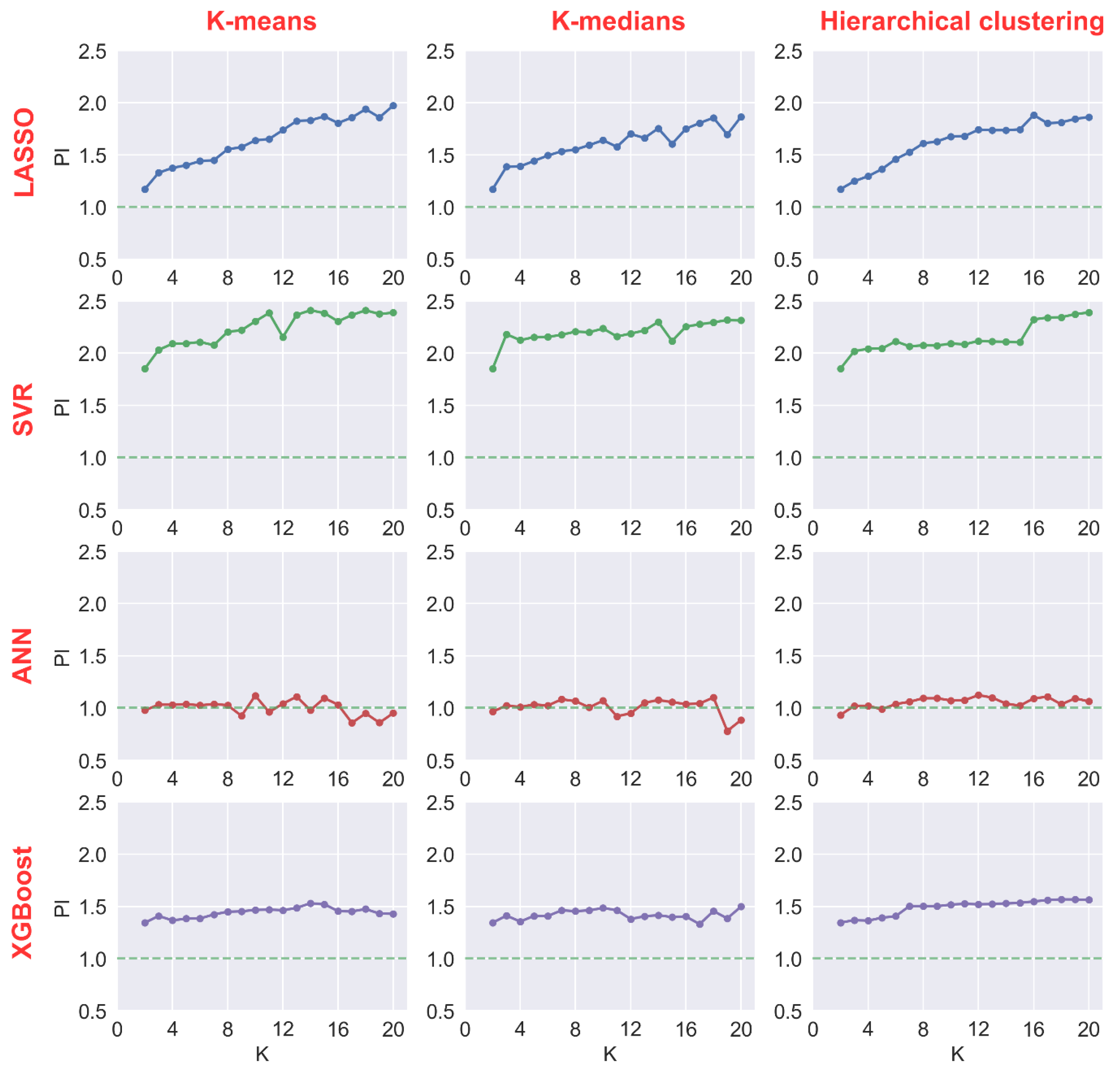
4.1. Performance Improvement by Integrating Clustering

As mentioned in Section 2.1, the proposed novel metric, performance improvement (PI), is used to compare the performance of ensemble models and the original regression models (with parameters optimization and performance being shown in

Table 3. Parameters optimization result and performance of different regression models.

Method	Parameters	Optimal Value	MAE	MAPE	RMSE
LASSO	Lambda	0.00001	37.96	26.87	61.79
SVR	Kernel function	RBF	34.5	21.74	64.37
	C	1
	Gamma	0.01
ANN	Hidden neurons	25	20.02	11.37	34.39
	Activation	Sigmoid
XGBoost	Number of estimators	140	21.87	12.22	40.36
	Learning rate	0.3
	Max depth	7

). A larger PI means a larger performance improvement of the new model (ensemble model) compared with the basic model (original regression model). The results are presented in Figure 8. Three columns indicate three clustering algorithms and four lines indicate four regression models. Each subfigure is the combination of these clustering algorithms and regression models.

In the first line of Figure 8, it can be observed that the PIs are larger than one, which means that all the three clustering algorithms can increase the performance of the LASSO regression model. This is reasonable as the original LASSO regression is a linear regression, while there is a nonlinear relationship in the prediction task. After clustering, the data in one group could have a higher linear relationship, which can technically improve the prediction performance. It can also be found that the PI increases gradually with the increase in K and the limitation of this trend is near 18. In fact, this trend becomes smooth when K is larger than 12. Therefore, the tradeoff between prediction performance and computation cost should be considered in real applications.

In the second line of Figure 8, it can be observed that the PIs are larger than that in the first line with a certain K value and clustering algorithm. This means that clustering algorithms can improve the performance of SVR models more significantly compared with the LASSO regression. It can also be found that PI increases gradually with the increase in K, while this trend is not that significant when K is large. The reason for the great improvement in integrating clustering algorithms on top of SVR is explained as follows. First, the general benefit brought by clustering is that data in each group could have a high similarity, which is favorable for regression. Second, clustering algorithms can divide the original data into different groups so each group has a smaller amount of sample. This is very favorable for SVR because it does not need all the data to find the hyperplane. In addition, a smaller amount of data can avoid the problem of high mapping dimensions for the kernel function. Thus, better performance and strong generalization ability can be obtained.

In the third line of Figure 8, it can be observed that the PIs are near one. This means that clustering algorithms cannot significantly increase the performance of the ANN model. In some cases, with a large K (for K-means and K-medians), PIs are even smaller than one. One possible reason is that too many clusters can reduce the information contained in each cluster, which may not be sufficient to fully train the ANN model.

In the fourth line of Figure 8, it can be observed that the PIs are slightly larger than one. In addition, the increase in K cannot further significantly increase the PI. The reason can be explained as follows. XGBoost itself is an ensemble model of decision trees with classification functions. Therefore, the previous clustering analysis only has little effect on the prediction performance of XGBoost.

In summary, the performance improvement by integrating clustering on different regression models from high to low is SVR, LASSO, XGBoost, and ANN. For the comparison of columns, there is no significant difference between these three clustering algorithms (K-means, K-medians, and Hierarchical clustering). More work is then conducted to find whether it is because of the high similarity among the results of different clustering algorithms.

Table 4. The maximum and minimum amount of data in clusters when K = 2, K = 5, K = 10, and K = 20.

Cluster Number	Maximum/Minimum and Proportion	K-Means	K-Medians	Hierarchical Clustering
K = 2	Maximum	31,104	31,104	31,104
	Proportion	71.01%	71.01%	71.01%
	Minimum	12696	12696	12696
	Proportion	28.99%	28.99%	28.99%
K = 5	Maximum	12674	12633	19268
	Proportion	28.94%	28.84%	43.99%
	Minimum	2477	4869	321
	Proportion	5.65%	11.12%	0.73%
K = 10	Maximum	7156	8461	12375
	Proportion	16.34%	19.32%	28.25%
	Minimum	1865	2328	58
	Proportion	4.26%	5.31%	0.13%
K = 20	Maximum	4095	4704	8845
	Proportion	9.35%	10.74%	20.19%
	Minimum	54	326	13
	Proportion	0.12%	0.74%	0.03%

shows the maximum and minimum amount of data in clusters when K = 2, K = 5, K = 10, and K = 20. Figure 9 also illustrates the result when K = 2 and K = 5. It can be found that when K = 2, all the methods can properly divide the data into working day data and nonworking day data. That is also the reason why there is a great performance improvement when K = 2 compared to when no clustering method is used (shown in Figure 8). With the increase in the number of clusters, the result of Hierarchical clustering especially shows a great difference from the other methods. This means that different unobvious patterns can be found by different cluster methods. These new patterns can also improve the prediction performance of the ensemble model. However, the performance improvement is not that significant compared with the case when the obvious patterns are found (i.e., working day and nonworking day).

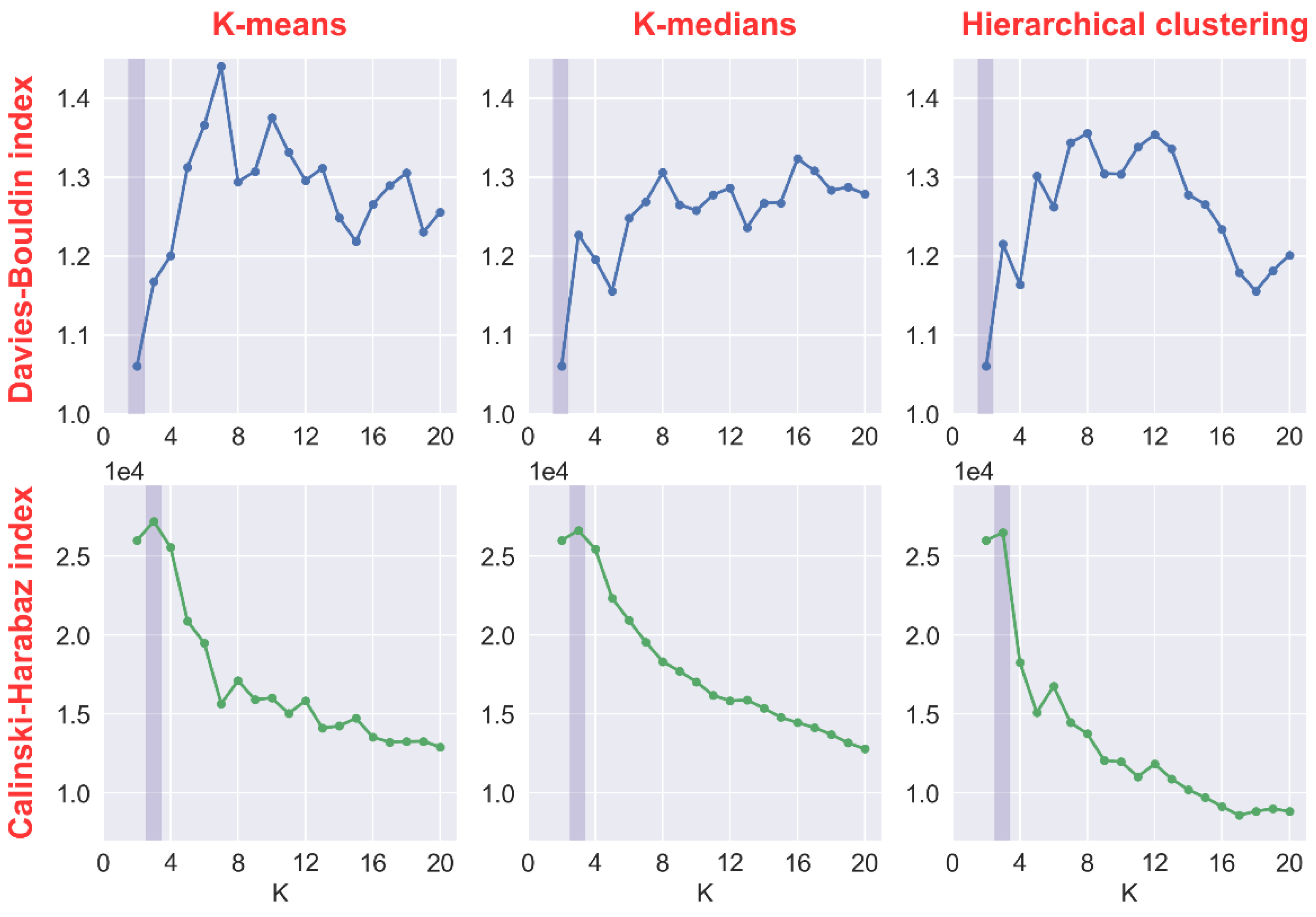
4.2. Optimal Cluster Number

Figure 10 presents the variation in Davies–Bouldin index (DBI) and Calinski–Harabaz index (CHI) with the increase in cluster number. These indexes are used to decide the optimal cluster number in previous studies [22,24]. As mentioned in Section 2.5.1, the lowest value of DBI and the highest value of CHI indicate the optimal cluster number. Therefore, it can be observed from the figure that the optimal cluster number determined by the Davies–Bouldin index (DBI) and Calinski–Harabaz index (CHI) are 2 and 3, respectively, regardless of the clustering algorithms. Compared with the result in Figure 8, it can be found that 2 or 3 are quite close to the optimal cluster number of ANN and XGBoost. However, they are not close to the optimal cluster number of LASSO and SVR, especially for LASSO. In real applications, clustering evaluation metrics can be first used to estimate the optimal cluster number for LASSO and SVR, and more clusters can be tried after considering the tradeoff between prediction performance and computation cost.

4.3. Performance of Different Models in Energy Consumption Prediction Task

In this section, the performances of different ensemble models are compared to find the best model for short-term forecasting of building energy consumption. As mentioned in Section 2.1, to facilitate the comparison among different ensemble models, the performance of the Autoregressive Integrated Moving Average (ARIMA) is selected as a baseline. The performances of the best ensemble models for different regression algorithms are summarized in

Table 5. Performance of the best ensemble models for different regression algorithms.

	ARIMA	LASSO	SVR	ANN	XGBoost
Clustering Algorithm		K-Means	K-Means	Hierarchical Clustering	Hierarchical Clustering
MAE	29.86	21.65	16.32	19.13	14.94
MAPE	13.68	11.65	8.15	10.26	7.51
RMSE	54.71	33.21	26.27	28.42	25.06
PI vs. ARIMA	1.00	1.40	1.86	1.61	2.00

.

The performance of regression models integrated with clustering algorithms from high to low is XGBoost (integrated with Hierarchical clustering with a PI of 2.00 compared with ARIMA), SVR (integrated with K-means with a PI of 1.86 compared with ARIMA), ANN (integrated with Hierarchical clustering with a PI of 1.61 compared with ARIMA), and LASSO (integrated with K-means with a PI of 1.40 compared with ARIMA). It is found that although clustering algorithms can most significantly improve the performance of SVR, XGBoost and Hierarchical outperform SVR and K-means. The reason is that the performance of XGBoost is much better than that of the SVR model.

In summary, because of the working patterns of the building, the use of the ensemble model (clustering and regression model) is favorable for the prediction of building power consumption. For the cluster number, when the obvious pattern is found by the clustering algorithm, there is a great performance improvement. When the cluster number further increases, the increase in unobvious patterns can also increase the performance of the ensemble model. However, two aspects need to be considered. First, increasing the number of clusters reduces the information of data in each cluster, which may not be sufficient for training the regression model. Second, the tradeoff between prediction performance and computation cost should be considered in real applications.

5. Conclusions

In this study, based on a practical requirement of a green office building in Shenzhen, a comprehensive study is conducted to systematically study the integration of clustering and regression and answer the questions that are not well explained. A performance evaluation index dedicated to comparing the performance of two prediction models is proposed. The main conclusions are as follows.

• In general, integrating clustering with regression can effectively improve the prediction performance of the regression model. In this study, the results show that the performance improvement by integrating clustering with different regression models from high to low is SVR, LASSO, XGBoost, and ANN. More specifically, integrating clustering almost has a negligible impact on the ANN model.
• The optimal cluster number determined by clustering evaluation metrics may not be the optimal number for the ensemble model (integration of clustering and regression). In this study, the optimal cluster numbers determined by clustering evaluation metrics are quite close to the optimal numbers of ANN and XGBoost. However, they are not closed to the optimal numbers of LASSO and SVR, especially for LASSO.
• In this study, there is no great difference among clustering methods (K-means, K-medians, and Hierarchical clustering) in the task of short-term building energy consumption prediction.
• In this study of predicting the energy consumption of the coming hour, the performance of different regression models integrated with clustering algorithms from high to low is XGBoost, SVR, ANN, and LASSO.

There are some limitations of this study. In this work, only the variables in the previous hour are used. In fact, the data in the past few hours could be considered, which may further increase the performances of models. The outdoor temperature is not included in the model inputs, due to the absence of data. In the future, more measured data of different buildings will be studied to further demonstrate the findings in this study and draw more general and concrete conclusions.

References

1. Lu, W.; Tam, V.W.; Chen, H.; Du, L. A holistic review of research on carbon emissions of green building construction industry. Eng. Constr. Arch. Manag. 2020, 27, 1065–1092. [Google Scholar] [CrossRef]
2. Kneifel, J.; Webb, D. Predicting energy performance of a net-zero energy building: A statistical approach. Appl. Energy 2016, 178, 468–483. [Google Scholar] [CrossRef] [Green Version]
3. Walker, S.; Labeodan, T.; Boxem, G.; Maassen, W.; Zeiler, W. An assessment methodology of sustainable energy transition scenarios for realizing energy neutral neighborhoods. Appl. Energy 2018, 228, 2346–2360. [Google Scholar] [CrossRef]
4. Ramesh, T.; Prakash, R.; Shukla, K.K. Life cycle energy analysis of buildings: An overview. Energy Build. 2010, 42, 1592–1600. [Google Scholar] [CrossRef]
5. Lu, X.; Hinkelman, K.; Fu, Y.; Wang, J.; Zuo, W.; Zhang, Q.; Saad, W. An Open Source Modeling Framework for Interdependent Energy-Transportation-Communication Infrastructure in Smart and Connected Communities. IEEE Access 2019, 7, 55458–55476. [Google Scholar] [CrossRef]
6. Liu, Y.; Liang, J.; Wang, X.; Ouyang, Y. Status, Problems and Countermeasures of Energy-Saving Assessment for Building Energy-Saving Projects. Sustain. Dev. 2013, 3, 116–122. [Google Scholar]
7. Turner, C.; Frankel, M. Green Building Performance Evaluation: Measured Results from LEED New Construction Buildings; Texas A&M University: College Station, TX, USA, 2008. [Google Scholar]
8. Chen, Z.; Chen, Y.; Xiao, T.; Wang, H.; Hou, P. A novel short-term load forecasting framework based on time-series clustering and early classification algorithm. Energy Build. 2021, 251, 111375. [Google Scholar] [CrossRef]
9. Wang, H.; Xu, P.; Lu, X.; Yuan, D. Methodology of comprehensive building energy performance diagnosis for large commercial buildings at multiple levels. Appl. Energy 2016, 169, 14–27. [Google Scholar] [CrossRef]
10. Dong, Z.; Zhu, P.; Bobker, M.; Ascazubi, M. Simplified Characterization of Building Thermal Response Rates. Energy Procedia 2015, 78, 788–793. [Google Scholar] [CrossRef]
11. Wang, Y.; Shen, Y.; Mao, S.; Chen, X.; Zou, H. LASSO and LSTM Integrated Temporal Model for Short-Term Solar Intensity Forecasting. IEEE Internet Things J. 2018, 6, 2933–2944. [Google Scholar] [CrossRef]
12. Paudel, S.; Elmitri, M.; Couturier, S.; Nguyen, P.H.; Kamphuis, R.; Lacarrière, B.; Le Corre, O. A relevant data selection method for energy consumption prediction of low energy building based on support vector machine. Energy Build. 2017, 138, 240–256. [Google Scholar] [CrossRef]
13. Zhang, F.; Deb, C.; Lee, S.E.; Yang, J.; Shah, K.W. Time series forecasting for building energy consumption using weighted Support Vector Regression with differential evolution optimization technique. Energy Build. 2016, 126, 94–103. [Google Scholar] [CrossRef]
14. Azadeh, A.; Ghaderi, S.F.; Sohrabkhani, S. Annual electricity consumption forecasting by neural network in high energy consuming industrial sectors. Energy Convers. Manag. 2008, 49, 2272–2278. [Google Scholar] [CrossRef]
15. Kalogirou, S.A. Artificial neural networks in energy applications in buildings. Int. J. Low-Carbon Technol. 2006, 1, 201–216. [Google Scholar] [CrossRef]
16. Xue, P.; Jiang, Y.; Zhou, Z.; Chen, X.; Fang, X.; Liu, J. Multi-step ahead forecasting of heat load in district heating systems using machine learning algorithms. Energy 2019, 188, 116085. [Google Scholar] [CrossRef]
17. Yang, J.; Ning, C.; Deb, C.; Zhang, F.; Cheong, D.; Lee, S.E.; Sekhar, C.; Tham, K.W. k-Shape clustering algorithm for building energy usage patterns analysis and forecasting model accuracy improvement. Energy Build. 2017, 146, 27–37. [Google Scholar] [CrossRef]
18. Karijadi, I.; Chou, S.Y.; Dewabharata, A.; Cheng, R.G. Electricity Load Prediction using Fuzzy c-means Clustering EMD based Support Vector Regression for University Building. In Proceedings of the 2019 International Conference on Fuzzy Theory and Its Applications (iFUZZY), New Taipei, Taiwan, 7–10 November 2019; pp. 163–168. [Google Scholar]
19. Li, X.; Deng, Y.; Ding, L.; Jiang, L. Building cooling load forecasting using fuzzy support vector machine and fuzzy C-mean clustering. In Proceedings of the International Conference on Computer & Communication Technologies in Agriculture Engineering, Chengdu, China, 12–13 June 2010. [Google Scholar]
20. Zhou, Z. Hybrid Modeling of Central Air-Conditioning Cold Source System Energy Consumption with K-means Cluster Algorithm. IOP Conf. Ser. Earth Environ. Sci. 2019, 295, 52035. [Google Scholar] [CrossRef]
21. Zheng, H.; Wu, Y. A XGBoost Model with Weather Similarity Analysis and Feature Engineering for Short-Term Wind Power Forecasting. Appl. Sci. 2019, 9, 3019. [Google Scholar] [CrossRef] [Green Version]
22. Luo, X. A novel clustering-enhanced adaptive artificial neural network model for predicting day-ahead building cooling demand. J. Build. Eng. 2020, 32, 101504. [Google Scholar] [CrossRef]
23. Chen, H.; Wang, S.; Tian, Y. A new approach for power-saving analysis in consumer side based on big data mining. In Proceedings of the 2018 IEEE Power & Energy Society General Meeting (PESGM), Portland, OR, USA, 5–10 August 2018. [Google Scholar]
24. Wang, Y.; Liu, Y.; Li, L.; Infield, D.; Han, S. Short-Term Wind Power Forecasting Based on Clustering Pre-Calculated CFD Method. Energies 2018, 11, 854. [Google Scholar] [CrossRef] [Green Version]
25. Voyant, C.; Notton, G.; Kalogirou, S.; Nivet, M.-L.; Paoli, C.; Motte, F.; Fouilloy, A. Machine learning methods for solar radiation forecasting: A review. Renew. Energy 2017, 105, 569–582. [Google Scholar] [CrossRef]
26. Bartholomew, D.J. Time Series Analysis Forecasting and Control; JSTOR: New York, NY, USA, 1971. [Google Scholar]
27. Bourdeau, M.; Zhai, X.Q.; Nefzaoui, E.; Guo, X.; Chatellier, P. Modeling and forecasting building energy consumption: A review of data-driven techniques. Sustain. Cities Soc. 2019, 48, 101533. [Google Scholar] [CrossRef]
28. Raju, V.N.G.; Lakshmi, K.P.; Jain, V.M.; Kalidindi, A.; Padma, V. Study the Influence of Normalization/Transformation Process on the Accuracy of Supervised Classification. In Proceedings of the 2020 Third International Conference on Smart Systems and Inventive Technology (ICSSIT), Tirunelveli, India, 20–22 August 2020. [Google Scholar]
29. Morán, A.; Fuertes, J.J.; Prada, M.A.; Alonso, S.; Barrientos, P.; Díaz, I.; Domínguez, M. Analysis of electricity consumption profiles in public buildings with dimensionality reduction techniques. Eng. Appl. Artif. Intell. 2013, 26, 1872–1880. [Google Scholar] [CrossRef]
30. Fan, C.; Xiao, F.; Zhao, Y. A short-term building cooling load prediction method using deep learning algorithms. Appl. Energy 2017, 195, 222–233. [Google Scholar] [CrossRef]
31. Edelmann, D.; Móri, T.F.; Székely, G.J. On relationships between the Pearson and the distance correlation coefficients. Stat. Probab. Lett. 2020, 169, 108960. [Google Scholar] [CrossRef]
32. Efron, B.; Tibshirani, R.J. An Introduction to the Bootstrap; Chapman & Hall: New York, NY, USA, 1993; p. 436. [Google Scholar]
33. MacQueen, J. Some methods for classification and analysis of multivariate observations. In Proceedings of the Fifth Berkeley Symposium on Mathematical Statistics and Probability, Oakland, CA, USA, 1 January 1967; pp. 281–297. [Google Scholar]
34. Bradley, P.S.; Mangasarian, O.L.; Street, W.N. Clustering via concave minimization. Adv. Neural Inf. Process. Syst. 1997, 9, 368–374. [Google Scholar]
35. Nikolaou, T.G.; Kolokotsa, D.; Stavrakakis, G.S.; Skias, I.D. On the Application of Clustering Techniques for Office Buildings’ Energy and Thermal Comfort Classification. IEEE Trans. Smart Grid 2012, 3, 2196–2210. [Google Scholar] [CrossRef]
36. Tibshirani, R. Regression shrinkage and selection via the lasso. J. R. Stat. Soc. Ser. B 1996, 58, 267–288. [Google Scholar] [CrossRef]
37. Vapnik, V.; Golowich, S.E.; Smola, A. Support vector method for function approximation, regression estimation, and signal processing. Adv. Neural Inf. Process. Syst. 1997, 281–287. [Google Scholar] [CrossRef]
38. Vapnik, V. The Nature of Statistical Learning Theory; Springer: Berlin/Heidelberg, Germany, 1999. [Google Scholar]
39. Chen, T. Introduction to Boosted Trees; University of Washington Computer Science: Seattle, DC, USA, 2014; Volume 22, pp. 14–40. [Google Scholar]
40. Natekin, A.; Knoll, A. Gradient boosting machines, a tutorial. Front. Neurorobotics 2013, 7, 21. [Google Scholar] [CrossRef] [PubMed] [Green Version]
41. Friedman, J.H. Stochastic gradient boosting. Comput. Stat. Data Anal. 2002, 38, 367–378. [Google Scholar] [CrossRef]
42. Davies, D.L.; Bouldin, D.W. A cluster separation measure. IEEE Trans. Pattern Anal. Mach. Intell. 1979, 1, 224–227. [Google Scholar] [CrossRef]
43. Caliński, T.; Harabasz, J. A dendrite method for cluster analysis. Commun. Stat.-Theory Methods 1974, 3, 1–27. [Google Scholar] [CrossRef]
44. Wang, H.; Lu, X.; Xu, P.; Yuan, D. Short-term Prediction of Power Consumption for Large-scale Public Buildings based on Regression Algorithm. Procedia Eng. 2015, 121, 1318–1325. [Google Scholar] [CrossRef] [Green Version]
45. Garreta, R.; Moncecchi, G. Learning Scikit-Learn: Machine Learning in Python; Packt Publishing: Birmingham, UK, 2013. [Google Scholar]
46. Karatzoglou, A.; Meyer, D.; Hornik, K. Support Vector Machines in R. J. Stat. Softw. 2006, 15, 1–28. [Google Scholar] [CrossRef]
Figure 1. Research outline of the study.
Buildings 12 01701 g001
Figure 2. Schematic of the bootstrap method.
Buildings 12 01701 g002
Figure 3. Schematic of Hierarchical clustering algorithm.
Buildings 12 01701 g003
Figure 4. Schematic of Support Vector Regression.
Buildings 12 01701 g004
Figure 5. The green building of the case study.
Buildings 12 01701 g005
Figure 6. The energy management system of the green building.
Buildings 12 01701 g006
Figure 7. Pearson correlation coefficients of different variables in the green building.
Buildings 12 01701 g007
Figure 8. Performance improvement of different ensemble models (clustering and regression) compared with the corresponding original regression model.
Buildings 12 01701 g008
Figure 9. Cluster results when K = 2 and K = 5.
Buildings 12 01701 g009
Figure 10. Optimal cluster number determined by Davies–Bouldin index (DBI) and Calinski–Harabaz index (CHI).
Buildings 12 01701 g010