Stochastic Simulation of Mould Growth Performance of Wood-Frame Building Envelopes under Climate Change: Risk Assessment and Error Estimation

Abstract

Previous studies have shown that the effects of climate change on building structures will increase the mould growth risk of the wood-frame building envelope in many circumstances. This risk can be controlled by wind-driven rain deflection, improving water tightness of the exterior facade, and improving cladding ventilation. However, the effectiveness of these risk mitigation strategies are subject to various uncertainties, such as the uncertainties of wall component properties and micro-climatic conditions. The objective of this paper is to apply stochastic hygrothermal simulation to evaluate the mould growth risk of a brick veneer-clad wood-frame wall with a drainage cavity under historical and future climatic conditions of Ottawa, a Canadian city located in a cold climate zone. An extensive literature review was conducted to quantify the range of stochastic variables including rain deposition factor, rain leakage moisture source, cladding ventilation rate and material properties of brick. The randomised Sobol sequence-based sampling method, one of the Randomized Quasi-Monte Carlo (RQMC) methods, was applied for risk assessment and error estimation. It was found that, under the climatic condition of Ottawa, limiting the amount of wind-driven rain to which walls are subjected is a more robust mitigation measure than improving cladding ventilation in controlling mould growth risk, the improving of water tightness of exterior façade is not as robust as wind-driven rain deflection and cladding ventilation, however, the reduction of rainwater penetration can reduce the mould growth risk at different levels of rain deposition factor and cladding ventilation rate.

1. Introduction

Mould growth is one of the most important mechanisms of degradation that affects the durability performance of wood-frame building envelopes. It has been well recognised that climate change will bring more extreme weather conditions, such as severe rain events and heat waves [1,2], whereby, in the future, the effects from such weather conditions are anticipated to increase the mould growth risk of wood-frame building envelopes in many circumstances [3,4,5].

In 1999, Hazleden and Morris [6] proposed the 4-D (Defense) strategy for controlling and thereby reducing moisture-related issues including the mould growth in wood-frame building envelopes. The 4-D strategy includes the deflection of wind-driven rain (WDR) by use of roof overhangs; drainage of rainwater penetration by incorporating a drainage cavity; drying of accumulated rainwater through cladding ventilation, and, using moisture tolerant materials in the assembly. In past decades, there have been a considerable number of studies dealing with WDR deflection strategies [7,8,9], quantifying the amount of rainwater penetration [10,11,12], as well as evaluating the effect of cladding ventilation drying [13,14,15]. Recently, Brambila and Sangiorgio [16] conducted a comprehensive review of the impact of climate change on mould growth in energy-efficient buildings and potential mitigation strategies; they concluded that the control of wind-driven rain and the increase of cladding ventilation were important mitigation strategies to reduce the mould growth risk for wood-frame buildings in the future. However, there was still a lack of studies to evaluate the robustness of different mitigation or design strategies when they are exposed to various uncertainties such as uncertainties evident for material properties and climatic conditions, as well as the influence of other design parameters, particularly in consideration of climate change.

The stochastic approach can be applied in combination with hygrothermal simulation to investigate the mould growth risk of wood-frame wall assemblies exposed to different types of uncertainties, and thereby permit evaluating the robustness of proposed mitigation or design strategies. The application of stochastic modelling for uncertainty analysis of hygrothermal simulation can be traced back to 2001 when Salonvaara et al. [17] applied the Monte-Carlo (MC) method to investigate the influence of inexact material properties on simulation results. Zhao et al. [18] extended the MC analysis to boundary conditions, where both the material properties and boundary conditions were considered as stochastic variables to allow quantifying the uncertainty in the simulation results. As part of the activities of the IEA ANNEX 55 [19,20,21,22], a comprehensive probabilistic assessment framework was established to investigate the uncertainties of hygrothermal simulation and assess moisture problem risks. Thereafter, many researchers investigated the hygrothermal performance of wall assemblies using a probabilistic or stochastic simulation approach [23,24,25,26,27]. Recently, Wang and Ge [28] developed a stochastic modelling framework, which was intended to allow investigating moisture problem risks under different environmental or design scenarios. In this framework, the variables for both the environmental or design scenarios were considered as discrete variables, which could be organised by full factorial design, whereas, continuous stochastic variables were sampled using the Latin Hypercube Sampling method. Thereafter, the Latin Hypercube Sampling method and stochastic simulation were implemented within every scenario generated by factorial design to evaluate the moisture problem risk under each scenario. Hou et al. [29] investigated the freeze/thaw risk of masonry walls using four Randomized Quasi-Monte Carlo (RQMC) methods. They considered discrete variables (scenario variables) as stochastic variables as well, making them evenly mixed with continuous stochastic variables for stochastic simulation. Then the stochastic results were categorised into different scenarios, i.e., climatic conditions or the types of brick, by mapping the results to different discrete inputs to assess the freeze/thaw risk under each scenario. In addition, the error estimation of the stochastic results could be implemented for different sample sizes.

When the number of scenario variables increases, the number of simulations will increase considerably. For example, Gaur et al. [30] generated 15 realisations of 31-year climate data sets for one historical and 7 future climatological periods across 12 Canadian cities, which can be used for assessing the impact of climate change on building performance. To implement stochastic simulation, the climatic realisation could be considered as a scenario variable, however, the total number of stochastic simulations will be 15 times the number of stochastic simulations under each climatic realisation. Therefore, the computational cost will be further increased if the climatic realisations are combined with other scenario variables, e.g., wall orientations, to complete a full factorial design.

In this paper, it is intended that computational efficient stochastic simulation, which is based on Randomized Quasi-Monte Carlo (RQMC) methods, be applied to assess the mould growth risk of a wood-frame building envelope using red matt clay brick as cladding under different climatic realisations, wall orientations, and using different mould growth mitigation strategies. Such strategies could include e.g., control of rain deposition, rain leakage, or the use of cladding ventilation. The risk assessment was based on the historical and future climatic conditions of Ottawa, a Canadian city located in a cold climate zone.

2. Methods

To investigate the uncertainties of hygrothermal simulation and assess the mould growth risk, a baseline hygrothermal model was created. The 1-D hygrothermal model of a typical wood-frame wall was generated using Delphin 5.9.6, a widely used hygrothermal simulation program [31]. A comprehensive literature review was conducted to quantify the range of the stochastic variables: rain deposition factor, rain leakage moisture source and cladding ventilation rate, as well as the material properties of brick, i.e., water absorption coefficient and effective saturation water content. A literature review was also performed for different sampling methods, which largely determine the efficiency and reliability of the stochastic simulation. Based on the literature review, the randomized Sobol sequence-based sampling, one of the Randomized Quasi-Monte Carlo (RQMC) methods, was selected for stochastic simulation. The standard error of the stochastic results, i.e., mean value and standard deviation of the mould growth index, was evaluated at different sample sizes for different climatic realisations and wall orientations. The robustness of different risk control strategies was evaluated under the orientation that has the highest mould growth index, with consideration of different climatic realisations and the uncertainties of material properties of brick. The following sections demonstrate the process of stochastic simulation, risk assessment as well as error estimation.

2.1. Hygrothermal Model

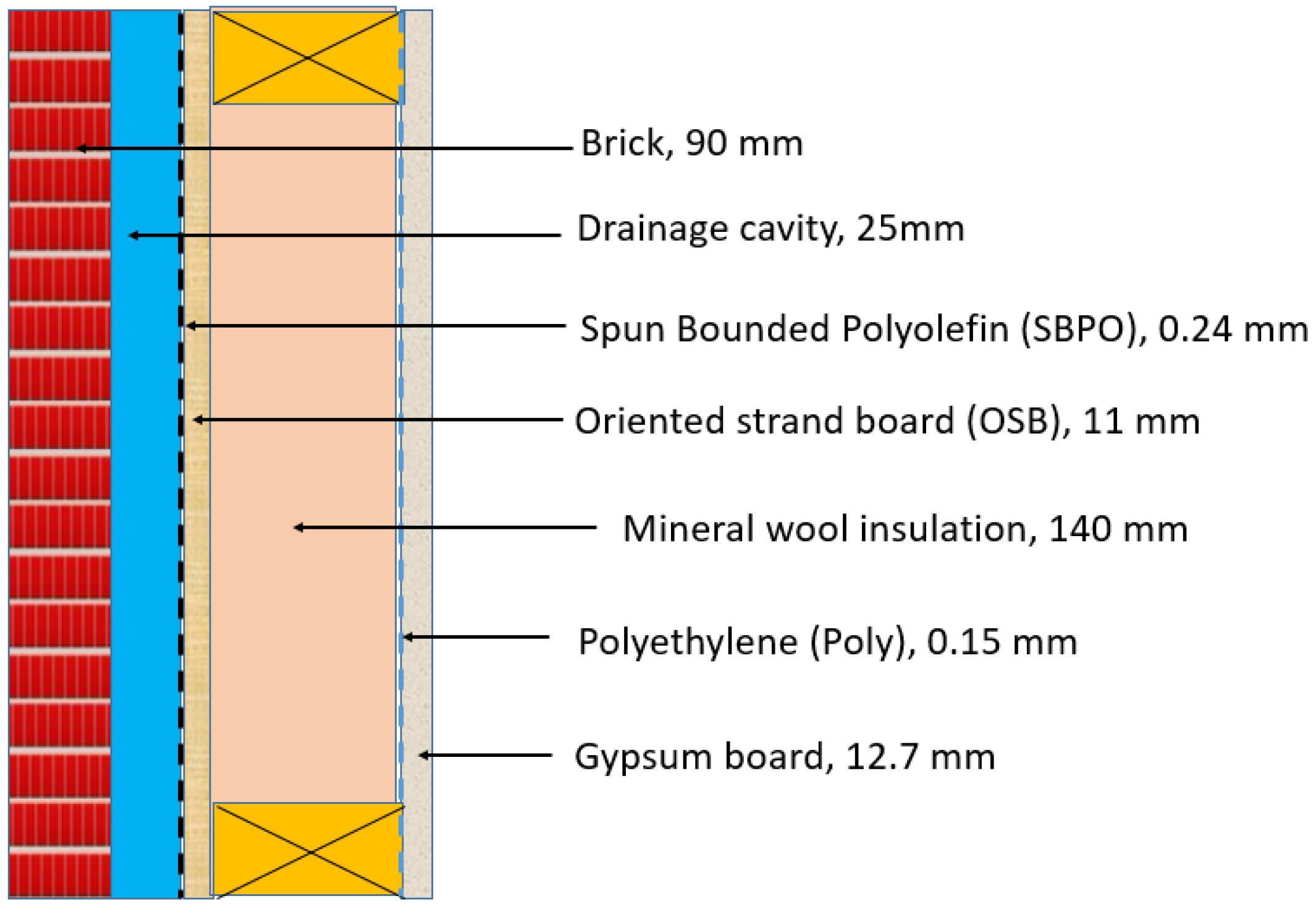
2.1.1. Wall Configuration and Material Properties

Figure 1 shows the wall configuration of the wood-frame wall investigated in this paper, and the basic properties of the materials used in the wall components are given in

Table 1. Basic material properties of the wall components.

	Bulk Density (kg/m3)	Porosity (m3/m3)	Effective Saturation Water Content (m3/m3)	Capillary Water Content (m3/m3)	Vapour Resistance Factor_Dry (−)	Water Absorption Coefficient (kg/m2s0.5)	Heat Capacity (J/kg·K)	Heat Conductivity (W/m·K)
Red matt clay brick	1935	0.265	0.217	0.162	129	0.0268	800	0.5
Air space	1.2	0.99	-	-	1	-	1006	0.025
SBPO *	464	0.012	0.012	0.01	305	0.00031	1250	0.248
OSB	650	0.4	0.38	0.27	753	0.0022	1880	0.094
Mineral wool	37	0.92	0.9	0.9	1.09	-	840	0.032
Polyethylene	1256	-	-	-	1 × 106	-	2100	0.16
Gypsum board	700	0.65	0.42	0.4	138	0.0019	870	0.16

* SBPO: Spun-bonded polyolefin.

. The material properties were taken from a series of NRC’s material property reports [32,33,34,35]. For the properties that were not found in NRC’s reports, these were taken from Delphin’s material database.

To reduce the number of stochastic material properties, a preliminary sensitivity analysis was performed to screen the influential material properties. The details of the sensitivity analysis can be found in [36]. It was found that the moisture storage function (scaled by effective saturation water content) and the liquid diffusivity (derived from effective saturation water content and water absorption coefficient) of brick are the most important material properties that influence the mould growth performance on OSB. Therefore in this paper, the effective saturation water content and the water absorption coefficient of the brick were considered as stochastic material properties.

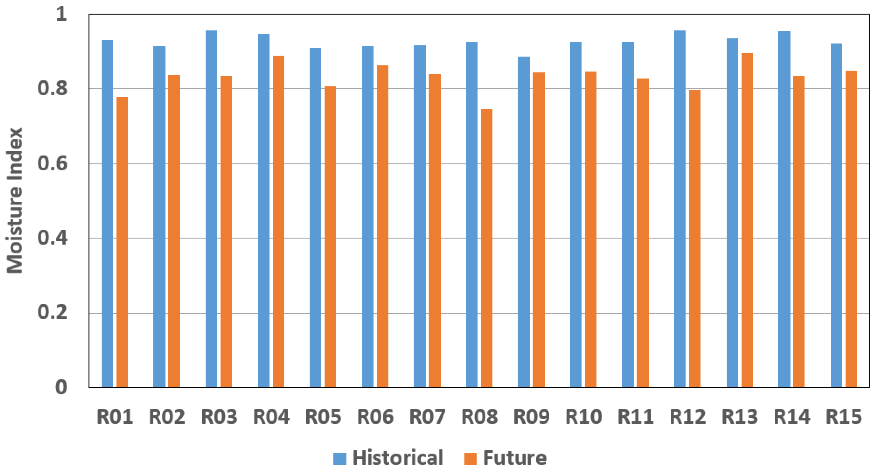
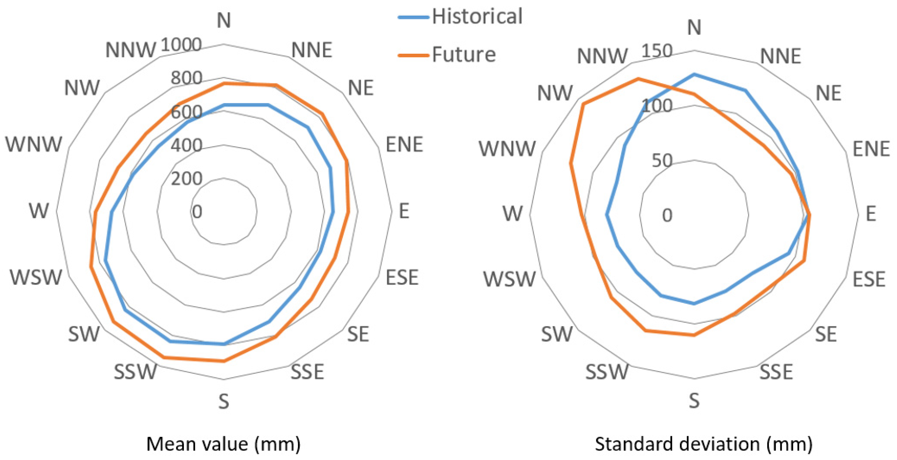
2.1.2. Boundary Conditions and Climatic Realisations

Table 2. Boundary conditions.

Interior Heat Transfer Coefficient (W/m2·K)	Interior Vapour Transfer Coefficient (s/m)	Short Wave Absorptivity (−)	Long Wave Emissivity (−)
8	1.52 × 10−8	0.6	0.9

shows the boundary conditions that were considered as constant values. The exterior heat and vapour transfer coefficients were set as dependent on wind speed according to EN ISO 6964 [37], and the dependency functions are given in Equations (1) and (2).

$${\mathrm{h}}_{\mathrm{ce}}=4+4\times \mathrm{v}$$

(1)

$${\mathsf{\beta }}_{\mathrm{ve}}=2.44·{10}^{-8}+2.44·{10}^{-8}\times \mathrm{v}$$

(2)

where

• h_ce—exterior heat transfer coefficient (W/m²·K)
• β_ve—exterior vapour transfer coefficient (s/m)
• v—wind speed (m/s)

The wind-driven rain deposited on the exterior wall surface was calculated based on the ASHRAE 160 model as given by Equation (3) [38]:

$${\mathrm{r}}_{\mathrm{bv}}={ \mathrm{F}}_{\mathrm{E}}\times { \mathrm{F}}_{\mathrm{D}}\times { \mathrm{F}}_{\mathrm{L}}\times \mathrm{U} \times \cos \mathsf{\theta } \times { \mathrm{r}}_{\mathrm{h}}$$

(3)

where

• r_bv—wind-driven rain deposited on the exterior wall surface
• F_E—rain exposure factor, reflects different exposure types, for buildings lower than 10 m; the rain exposure factor can be assumed to have a value of 1.4 for the severe exposure category, 1.0 for the medium exposure category, and 0.7 for the sheltered category
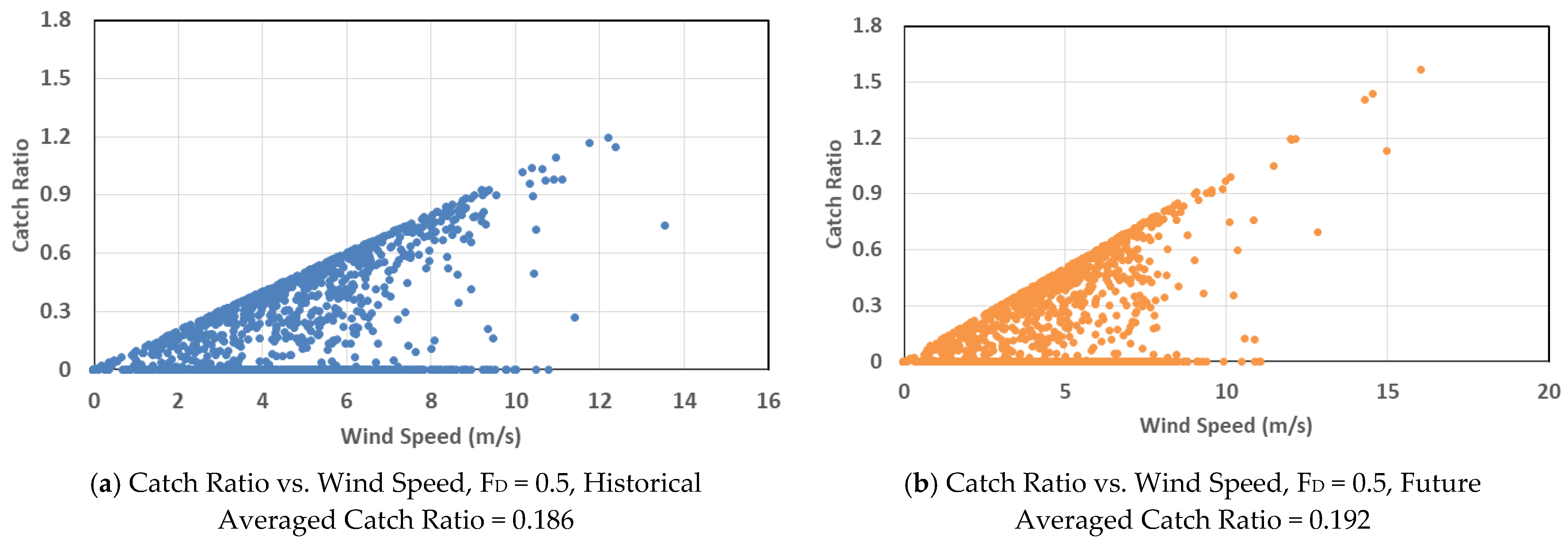
• F_D—rain deposition factor, reflects different roof designs; it can be assumed to have a value of 0.35 for a steep-slope roof, 0.5 for a low-slope roof and 1.0 for a wall subject to rain runoff
• F_L—empirical constant, 0.2 kg·s/(m³·mm)
• θ—angle between wind direction and normal to the wall
• U—hourly average wind speed at 10 m height, m/s
• r_h—rainfall intensity, horizontal surface, mm/h

In this paper, the rain exposure factor (F_E) was considered as 1, and the rain deposition factor (F_D) was considered as a stochastic variable. To simulate rain leakage, a moisture source was deposited on the exterior surface of the spun-bonded polyolefin (SBPO), and the quantity of this moisture source was considered as a stochastic variable as well. The effect of cladding ventilation was simulated using a source/sink approach, which considers the air in the drainage cavity as a heat and moisture source by imposing a cladding ventilation rate (ACH) that was considered as a stochastic variable. The range of these three stochastic variables and the stochastic brick properties will be discussed in Section 2.2.

The 15 climatic realisations of the 31-year climate data sets were generated for 12 Canadian cities, one baseline historical period (1986–2016) and 7 future scenarios with different levels of global warming; the details for the climate data generation can be found in [30]. In this paper, the historical climate data and the climate data with the worst future scenario for global warming (3.5 °C global warming) in the city of Ottawa were used for stochastic simulation (Hereafter, referred to as historical and future periods). To save computational costs, a 2-year moisture reference year was selected for each climatic realisation based on the moisture index, which was calculated year by year based on Equation (4) [39]:

$$\mathrm{MI}=\sqrt{{\left(1-\mathrm{DI}\right)}^2+{\mathrm{WI}}^2}$$

(4)

where

• MI—moisture index of a specific year
• DI—normalised drying index of a specific year
• WI—normalised wetting index of a specific year

The drying index represents the degree of moisture saturation of ambient air, whereas the wetting index considers the wind speed and horizontal rain. The absolute values of yearly WI and DI were calculated using Equations (5) and (6) [39]:

$$\mathrm{WI}={{\displaystyle \sum }}_1^{8760}\mathrm{U}\times {\mathrm{R}}_{\mathrm{h}}/1000$$

(5)

where

• U—wind speed in a specific hour, m/s
• R_h—horizontal rain in a specific hour, mm

$$\mathrm{DI}={{\displaystyle \sum }}_1^{8760}({\mathrm{w}}_{\mathrm{sat}}-\mathrm{w})$$

(6)

where

• w_sat—humidity ratio at saturation in a specific hour
• w—humidity ratio of ambient condition in a specific hour

The yearly values for DI and WI were normalised based on the maximum and minimum values in all the 15 realisations within one climatological period, to consider the relative difference amongst different realisations; thereafter, the moisture index was calculated for every single year for each 31-year climatic realisation. The selected 2-year moisture reference year include one 50 percentile and one 90 percentile of the moisture index in each 31-year climatic realisation. Finally, there were 15 realisations (R01, R02 … R15) of 2-year climate data sets for each climatological period, and the 15 realisations of 2-year climate data sets in each period were considered as discrete stochastic variables. Figure 2 shows the 2-year averaged moisture index of each climatic realisation in historical and future periods for Ottawa. It can be noted that the MIs were calculated based on DI and WI, which were values normalised within each climatological period. Therefore, the MIs reflect the relative difference amongst different climatic realisations, but, they do not reflect the difference between historical and future periods.

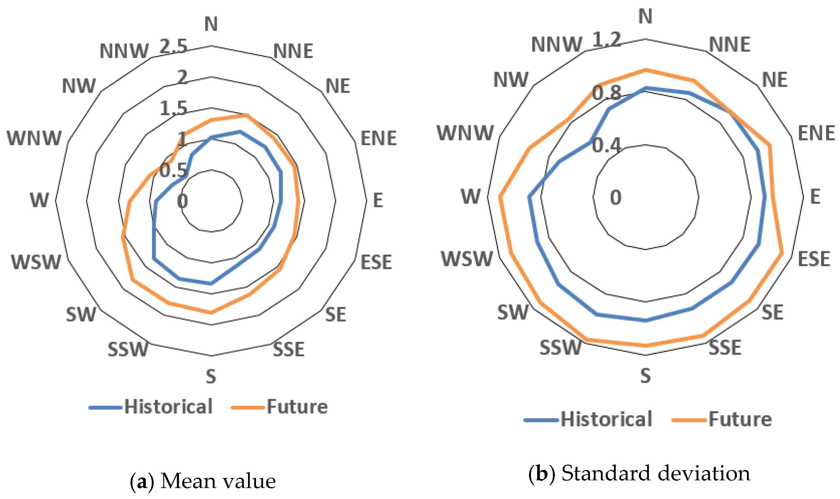
2.1.3. Wall Orientations

The wall orientations were assumed to follow a uniform distribution, which was distributed from 0° to 360°. The amount of wind-driven rain incidents on the wall varied depending on the orientation as shown in Figure 3.

The wind-driven rain for each orientation was calculated based on the use of the ASHRAE wind-driven rain model by assuming a rain deposition factor of 0.5 and a rain exposure factor of 1. According to the mean value of the 15 realisations, the SSW orientation receives the highest amount of wind-driven rain for both the historical and future periods; the orientation having the second-highest value is NNE. The North orientation has the highest standard deviation for the historical period, and the NW orientation has the highest standard deviation for the future period. The wind-driven rain distribution may largely influence the risk to mould growth for different orientations, however, the mould growth performance of the wall for each different orientation is a result of the combined effects of wind-driven rain and solar radiation.

2.2. Literature Review of Stochastic Variables

2.2.1. Rain Deposition Factor

Although ASHRAE 160 specifies three levels of rain deposition factor, that represent two types of roof design and one scenario of the wall subject to rainwater runoff, there is a lack of detailed information describing where the calculated wind-driven rain should be applied on the building façade, and each level of rain deposition factor reflects what level of overhang protection. To better understand the physical meaning of the rain deposition factor, a literature review was conducted for catch ratio, which is defined as the ratio of wind-driven rain to horizontal rain. Some important studies on quantifying catch ratio from which values we obtained are summarised in

Table 3. Literature review on catch ratio.

Authors	Year	Building Geometry 1	Approach	Catch Ratio	Notes
Choi [41]	1993	Bldg1, 4: 1: 1 Bldg2, 4: 8: 2	CFD simulation	Bldg1, 0.05–0.47, WS 2, 10 m/s; 0.34–1.17, WS, 20 m/s; Bldg2, 0–0.4, WS, 10 m/s; 0.04–0.82, WS, 20 m/s	The variation of catch ratio at each wind speed depends on the positions on the façade.
Blocken and Carmeliet [42]	2000	Bldg1, 4: 25: 7 Bldg2, 8: 25: 7	CFD simulation	Bldg1, 0–0.5 Bldg2, 0–0.4 WS, 0–6 m/s	Bldg 1 flat roof, Bldg 2 steep slope roof. The catch ratio is in a fixed position on the façade at middle height.
Blocken and Carmeliet [43]	2001	Same as above	CFD simulation & field measurement	Bldg1, 1.58 Bldg2, 1.26 WS, 10 m/s	The catch ratio is a specific catch ratio of 1 mm raindrop at the worst position on the façade-top edge.
Kubilay et al. [44]	2013	Tower building 35: 5: 4	CFD simulation & field measurement	Maximum specific catch ratio of 0.5 and 1 mm raindrop at 10 m/s WS is around 2.8	Averaged catch ratio at the worst position after two rain events are 0.3 and 0.5, respectively
Foroushani et al. [7]	2014	Cubic building 10: 10: 10	CFD simulation	0.6 at the worst position at WS 5 m/s	0.6 m overhang helps protect the upper half of the façade up to 80%
Kubilay et al. [9]	2017	19: 16: 8	CFD simulation	1.2 at the worst position at WS 10 m/s	A window sill with a size of 0.1 m reduces the catch ratio by 37%
Ge et al. [8]	2017	20: 39: 15	Field measurement	1.0 at the worst position at WS 8 m/s. Averaged catch ratio at worst position 0.213	0.6 m overhang reduces the catch ratio by 30% to 90% depending on different positions

¹ The dimensions listed in building geometry are height: length: width ² WS: Wind Speed.

. In general, the prevailing wind-driven rain orientation was selected for quantifying the catch ratio, and the buildings selected for measurement or simulation were located in a relatively exposed area. Although it has been well known that the catch ratio depends on both wind speed and rain intensity, the linear relationship between catch ratio and wind speed is much more significant than rain intensity [40]; accordingly, only the information on wind speed (WS) was provided in Table 3. Among the publications listed in Table 3, the maximum catch ratio, which represents the worst position on the façade, varies between 0.4 and 1.6 depending on the wind speed used for simulation and building geometry. However, according to field measurements, the averaged catch ratio value at the worst position after a rain event, or a period during field measurements is much lower than the catch ratio value at maximum wind speed. For example, Ge et al. [8] investigated the catch ratio and the effectiveness of the overhang of a mid-rise residential building in Vancouver through field measurements. The average catch ratio value at the worst position on the building over one year of measurements was 0.213, although the maximum catch ratio at a wind speed of 8 m/s was about 1.

Some studies have demonstrated the effectiveness of overhangs for protecting the building façade from wind-driven rain. According to the simulation study completed by Foroushani et al. [7], a 0.6-m overhang at the top edge of a cubic building can reduce the catch ratio at the upper half of the building by up to 80%. Ge et al. [8] further validated this conclusion from numerical simulations by field measurements; it was found that a 0.6-m overhang can reduce the catch ratio by 30% to 90% depending on the location on the façade. According to the results from numerical simulation undertaken by Kubilay et al. [9], even a window sill with a size of 0.1 m can decrease the catch ratio by up to 37%.

In this paper, the ASHRAE 160 semi-empirical model (Equation (3), rain exposure factor = 1) was used to calculate the wind-driven rain at the worst orientation (SSW) of the worst climatic realisation (2-year climate data) in the historical and future period (R03 for historical, R13 for future), then the hourly catch ratio was calculated to compare with the catch ratios listed in Table 3. Figure 4 shows the scatter plot of the wind-driven rain as a function of wind speed for F_D = 0.5 under historical and future periods. It can be seen that the maximum value for catch ratio, with F_D = 0.5 and WS = 10 m/s, is around 1. This value for the historical period is slightly lower than the values obtained from field measurement and numerical simulation for a mid-rise building [8,9], or low-rise building [43]. The value for catch ratio is higher for the future projected climate period as compared to the historical period, because of the higher projected wind speed in the future. The randomness of the scatter plot is due to the randomness of the wind direction, although most of the time the wind direction is normal to the facade. Therefore, the wind-driven rain calculated using the ASHRAE semi-empirical model, and with F_D = 0.5, can be considered as the amount of rain deposited on the façade at the worst position (top or top edge). Similarly, the hourly catch ratio values were also calculated for F_D = 0.35 and F_D = 1, the maximum and 2-years’ averaged catch ratio at these two levels of F_D were presented in

Table 4. Catch ratio for F_D = 0.35 and F_D = 1.

Rain Deposition Factor	Maximum Catch Ratio	Average Catch Ratio
0.35	Historical, 0.8; Future, 1.1	Historical, 0.129; Future, 0.135
1	Historical, 2.4; Future, 3.1	Historical, 0.371; Future, 0.384

. Since catch ratio with F_D = 0.35, is 30% lower than that with F_D = 0.5, the scenario of F_D = 0.35 can be considered as a moderate protection level, i.e., a 0.1-m overhang [9]. Whereas for the scenario with F_D = 1.0, this can be considered as the wall subject to rainwater runoff or the façade on a high-rise building, since the average catch ratio is around 0.38, which is very close to the average catch ratio of a tall building reported in the literature [44]. To consider the uncertainty of the building geometry, a small range of values for F_D was assigned for each level of F_D, whereby, the stochastic F_D value was categorised into three ranges: 0.35 to 0.56, to represent the wall with some protection; 0.56 to 0.78, to represent the wall without any protection, and; 0.78 to 1, to represent the wall subject to rainwater runoff or a wall in a high-rise building.

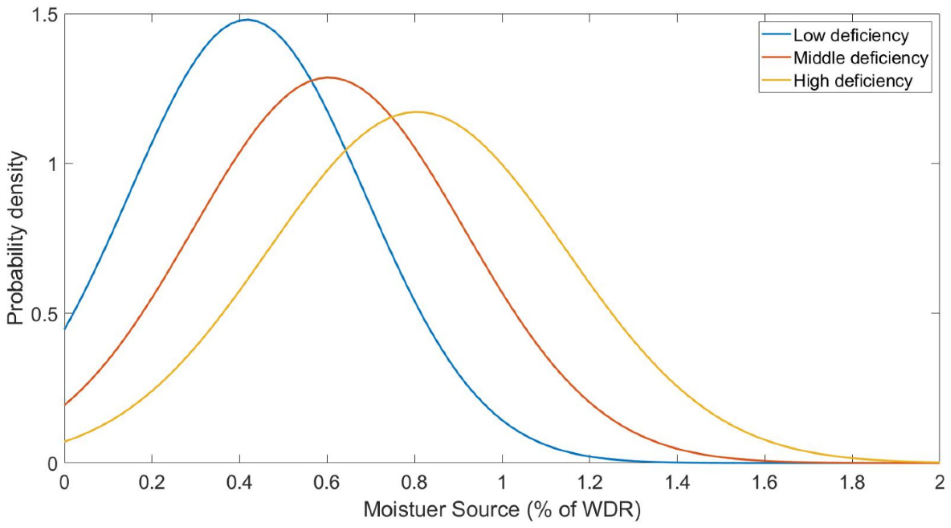
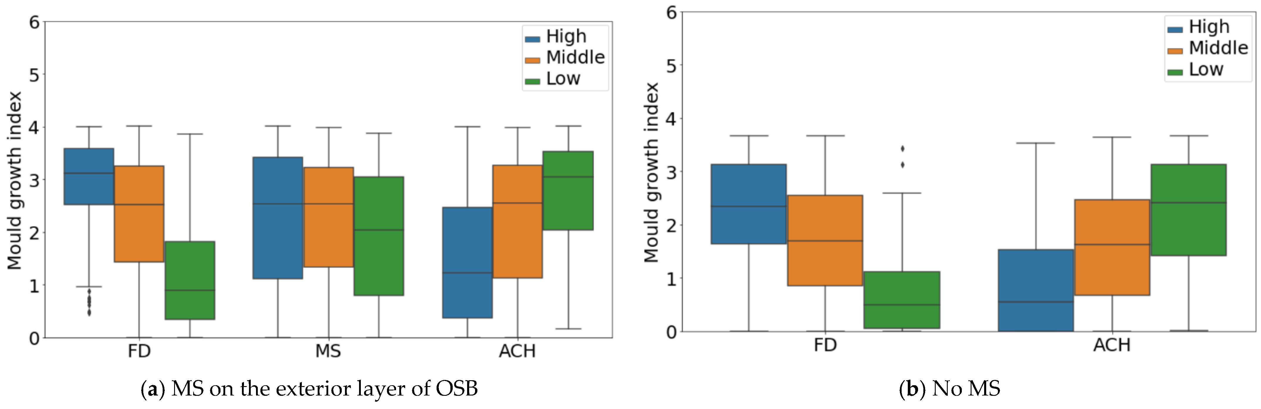
2.2.2. Moisture Source from Rain Leakage

To simulate the influence of rainwater penetration, ASHRAE 160 specifies 1% of wind-driven rain as a moisture source deposited on the water-resistive barrier if no other water entry information is available [38]. However, the amount of rainwater infiltration varies depending on different cladding types, water tightness levels, and climatic conditions including wind pressure and the amount of wind-driven rain. In general, water tightness tests can be applied to wall specimens to quantify the water infiltration rate at different levels of pressures and spray rates, representing the Driving Rain Wind Pressure (DRWP) and Wind Driven Rain (WDR) load in the atmosphere during rain events. The infiltrated water is then collected and measured to calculate the water infiltration rates. For most scenarios, the water infiltration rates of a test specimen are positively correlated with pressure differences across the wall assembly and the magnitude of the spray rates. For the water that has infiltrated into the wall assembly, it can be further distributed to either the interior surface of the cladding or the exterior surface of the sheathing membrane. Whilst, part of the infiltrated water would be drained away if a drainage cavity is present, Lacasse et al. [10] measured the distribution of infiltrated water at different locations, i.e., the interior side of the cladding and the exterior side of the sheathing membrane. It was found that, generally, the amount of water that reached the sheathing membrane of a wall assembly was ca. 15% of the total amount of water that penetrated the cladding and approximately 75% of this amount would be drained away if the wall had a drainage cavity. The greatest water penetration rate and the moisture source reached on the sheathing membrane for different types of wall assemblies as measured by Lacasse et al. [10] was summarised in

Table 5. Water entry rate of different types of wall assemblies (Data from reference [10]).

Wall Assembly	Drainage Cavity	Water Entry Rate (L/min)	Spray Rate (L/min)	1 Pressure (Pa)	Highest Water Entry Ratio	Moisture Source on Sheathing Membrane (SBPO)
Brick veneer	Yes	0.042	0.85	75	4.9%	0.7%
Stucco	Yes	0.191	1.7	0	11.2%	1.7%
Stucco	No
Fibre Board	Yes	0.15	0.85	150	17.6%	2.6%
Fibre Board	No	0.014	0.85	300	1.65%	0.25%
EIFS 2	No	0.218	3.4	300	6.41%	0.96%
Vinyl	No	0.059	0.85	300	6.94%	1%

¹ The pressure listed above was the pressure at which the highest water entry rate was obtained. In principle, a higher pressure will likely lead to a higher water entry rate, however, the water-tightness tests are subject to measurement uncertainties and the water entry rate for some deficiency types may not be sensitive to the applied pressure, therefore, the highest water entry ratio does not necessarily occur at the highest pressure. ² Exterior Insulation and Finish Systems.

.

Moore and Lacasse [45] further elaborated on the water entry characteristics and water retention characteristics of the cladding system from water entry and drainage tests. They developed a set of equations to derive the percentage of water retained in the cladding cavity. Recently, Xiao et al. [46] introduced a novel wind-driven rain pressure index, which allows one to calculate a series of weather-dependent water entry rates. Furthermore, Xiao et al. [47] demonstrated the procedure of fitting a water entry equation based on the water tightness test of a vinyl-clad wall.

In this paper, the water penetration was simulated by following the ASHRAE 160 approach, assuming a moisture source on the sheathing membrane; the moisture source amount (percentage of wind-driven rain) was considered as a stochastic variable. The probability distributions of the moisture source were determined through the following steps:

1. The hourly wind-driven rain pressure index (WDRPI) was calculated based on WDR and DRWP of 15 realisations of 31-year climatic data using Equation (7) [46]:

$$\mathrm{WDRPI}={ \mathrm{WDR}}^{\mathsf{\alpha }}\times {\mathrm{DRWP}}^{\mathsf{\beta }}$$

(7)

where:

• WDRPI—wind-driven rain pressure index
• WDR—wind-driven rain, calculated based on ASHRAE wind-driven rain model
• DRWP—driving-rain wind pressure, calculated by hourly wind velocity through Bernoulli’s principle
• α, β—for different configurations of wall assemblies based on their response to the WDR intensity and DRWP respectively during water tightness tests. For the brick wall, the value of α is 0.9506 and β is 1.0442.

2. The hourly moisture source reaching the sheathing membrane was calculated based on WDRPI and water entry Equation (8) [47]:

$$\mathrm{Moisture} \mathrm{source}= \mathrm{a}\times {\mathrm{WDRPI}}^{\mathrm{b}}$$

(8)

where:

• Moisture source—the amount of water that reaches the sheathing membrane per unit time (ml/min)
• a, b—adjustment coefficients derived from fitting the measured moisture source to corresponding values of WDRPIs. The details of the measurements and derivation of adjustment coefficients have been demonstrated based on a vinyl-clad wall by Xiao et al. [47]. The same procedure was also applied to the brick wall to obtain the two adjustment coefficients where: a = 7.998 × 10⁻⁶ and b = 0.6737.

3. The hourly moisture source was calculated from hourly WDR and hourly DRWP using steps 1 and step 2. The calculation was implemented for all the 15 climatic realisations of 31-year climatic data in the historical period, from which 4,073,400 data points of moisture source were generated.

A probability distribution of the moisture source was generated based on the hourly moisture source dataset that is including 4,073,400 data points. The unit of the calculated moisture source was converted to % of wind-driven rain by dividing the hourly wind-driven rain deposited on the exterior wall surface. Eventually, this probability distribution has a mean value of 0.56% and standard deviation of 0.35%, and the probability distribution was truncated above zero. Although the future climatic data had different WDR and DRWP from historical data, the calculated moisture source (percentage of wind-driven rain) for the future climatic condition was very close to the historical condition. Therefore, the same mean value and standard deviation were used for historical and future climatic conditions.

4. The water entry equation was developed based on a specific wall assembly with a deterministic deficiency level. To consider the uncertainty amongst different wall assembly types, another two probability distributions for moisture source were generated: one has a mean value of 0.3% to represent a relative lower deficiency level and another one has a mean value of 0.8% to represent a relative higher deficiency level. Both of these moisture sources nonetheless have a standard deviation value of 0.35%, since the variability of the moisture source under a specific deficiency level is primarily influenced by climatic conditions.

Figure 5 shows the three probability density functions, which were generated based on the mean values and standard deviation values of different wall deficiency levels assumed in steps 3 and step 4.

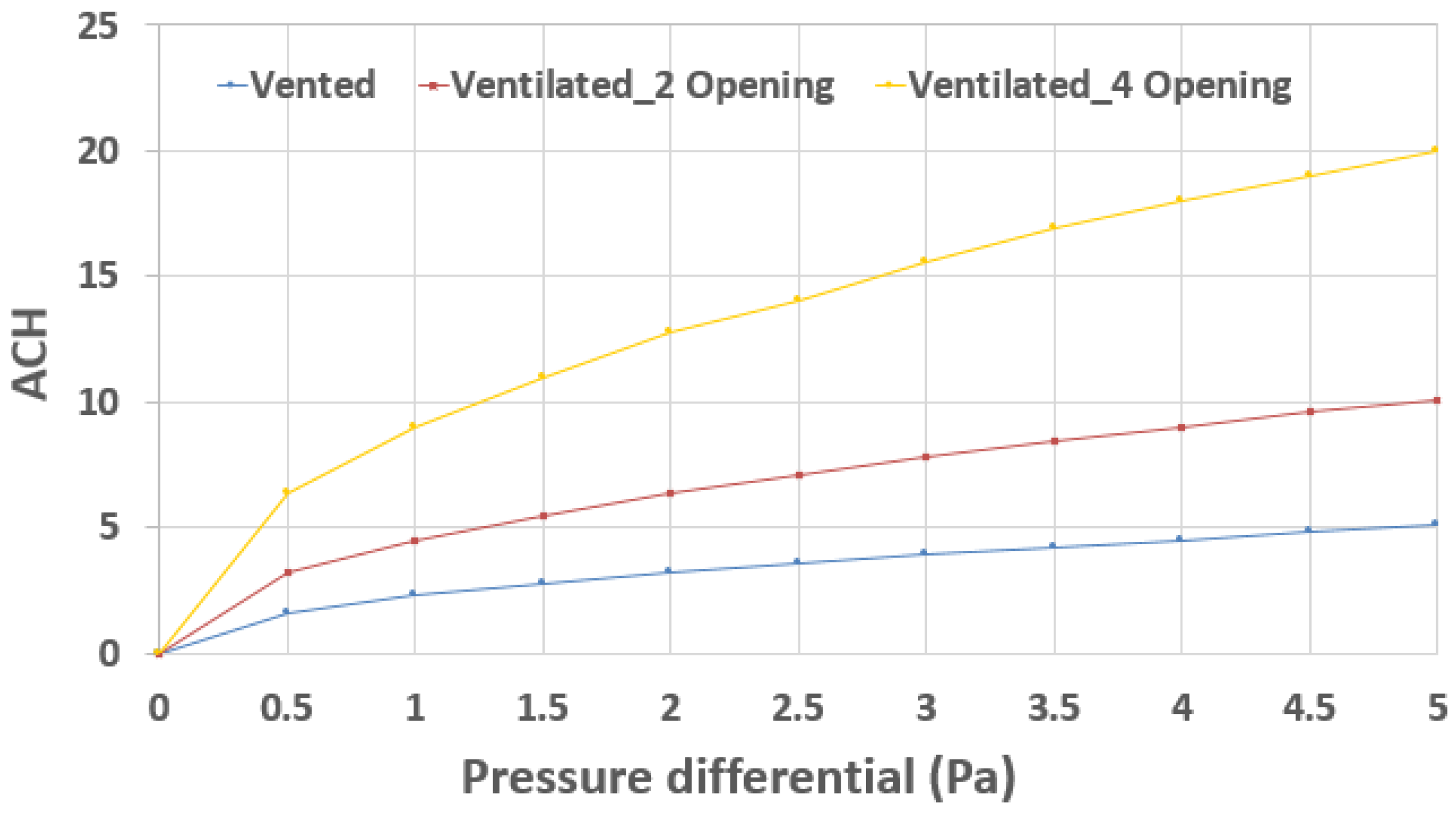
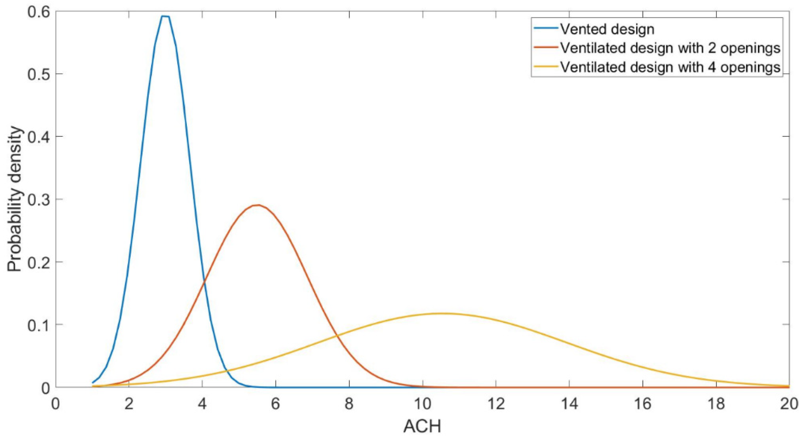
2.2.3. Cladding Ventilation Rate

The cladding ventilation rate (i.e., Air Changes per Hour, ACH) is influenced by the configuration of openings and local environmental conditions, i.e., wind-induced driving pressure and buoyancy induced driving pressure. Some of the literature in which are reported the ACH for brick assemblies is summarised in

Table 6. Literature review on cladding ventilation rate.

Authors	Year	Cladding	Cavity Depth (mm)	Opening	ACH
VanStraaten and Straube [48]	2004	Brick	20	1600 mm2 at top and bottom (2 of 10 × 80 at each position, clear no screen)	0–90
Finch and Straube [49]	2007	Brick	38	1300 mm2 at top & bottom (2 of 10 × 65 at each position, with bug screen)	0–9.6, Average 2.2
Ying Simpson [50]	2010	Brick1: 2.44 m height; Brick2: 4.88 m height	25	1560 mm2 on top (2 of 12 × 65 with bug screen); 1872 mm2 (2 of 12 × 78) on bottom	Brick 1: 1–11, Average 6; Brick 2: 1–6, Average 4.
Langmans et al. [14]	2016	Brick	40	1050 mm2 at top and bottom (2 of 15 × 35 at each position)	1 opening, 1–10, 85% of the time below 6; 2 openings, ACH doubled
Vanpachtenbeke et al. [51]	2020	Brick	40	1050 mm2 at top and bottom (2 of 15 × 35 at each position)	In between 5 and 10

.

Although there is a variety of opening designs found in literature, in Canada the most commonly used configuration for brick walls is two openings on the bottom and two openings at the top of the wall for every 1.2 m length of the wall assembly, with opening size varying between 600 to 900 mm² [49,50]. Generally, an insect screen is installed at the top openings, and the cavity depths are either 25 mm or 38 mm. This type of opening design leads to a variation of ACH between 0 and 10. For example, Finch and Straube reported the ACH of a brick wall with a 38 mm ventilated cavity, which was installed in the BEGHut, a test facility at the University of Waterloo. The ACH value was in the range of 0 to 9.6 with an average value of 2.2 for an entire year [49]. Simpson monitored the hygrothermal performance of a brick wall with a 25 mm ventilated cavity, which was located in the Burnaby campus of the British Columbia Institute of Technology (BCIT). The derived ACH value ranged between 1 and 11 with an average of 6 from February to June [50]. It is noted that the ACH can be increased up to 90 for a 20 mm deep cavity when there is no insect screen; however, this type of wall was only used for the experiment, walls 20 mm deep cavity without an insect screen is not a common construction practice in Canada [48].

Another cladding design for the brick wall is a vented cavity wall, which has no opening at the top but two openings on the bottom for every 1.2 m length of the wall. However, there is a lack of studies reporting the ventilation rate for vented brick wall cavity walls. Vanpachtenbeke et al. [51] investigated the non-ventilated brick wall where both the top and bottom openings were blocked. They found that the simulation with an ACH of 0 can produce similar vapour pressure in the cavity as that obtained from field measurements. Therefore, they concluded that poor airtightness of the wall does not lead to a significant drying potential and it can be ignored in hygrothermal simulations.

In this paper, the ACH for vented brick walls was calculated based on the procedure developed by Straube and Burnett [52]. The bottom opening size and the cavity dimension were assumed the same as in [50], and only one opening with blockage of insect screen was assumed on the top to simulate the potential air circulation between the bottom openings and small deficiencies on the façade. To explore the impact of increasing cladding ventilation, the ACH for 4 openings was also calculated. The pressure differential between the top and bottom was assumed to be varied from 0 to 5 Pa, with the highest frequency at 1.5 Pa based on the pressure differential reported in [50,52]. In Figure 6, the calculated values for ACH of a 25-mm cavity is shown for vented (2 openings on the bottom, no openings at the top), ventilated with 2 openings (2 openings on the bottom and top), and ventilated with 4 openings (4 openings on bottom and top) for a 1.2 × 2.4 m (length × height) brick wall. Then, the ACH at 1.5 Pa pressure differential was set as the mean value and the standard deviation values for different ventilation designs were quantified based on the range of ACH, from which, three probability distributions of ACH representing three cladding ventilation designs were generated, and the probability density functions were presented in Figure 7. The probability functions were truncated from 1 since the air in the cavity is less likely to be stagnant.

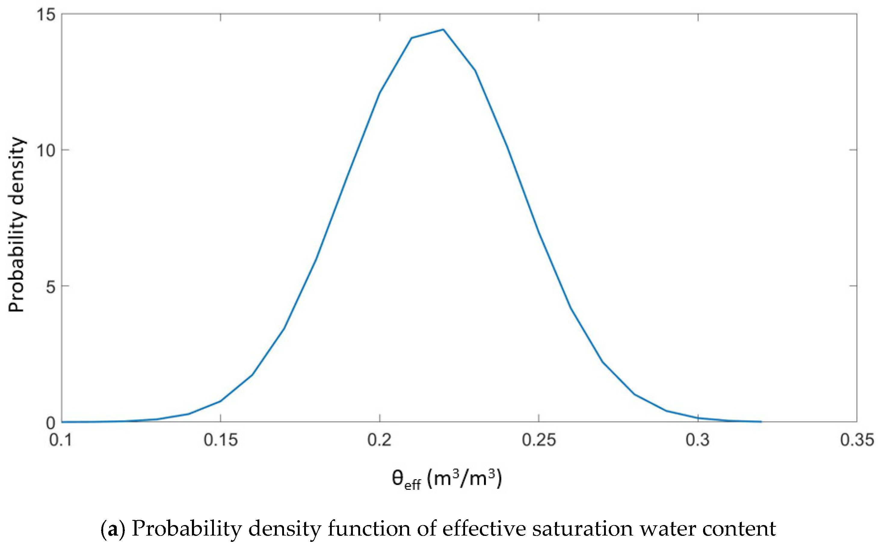
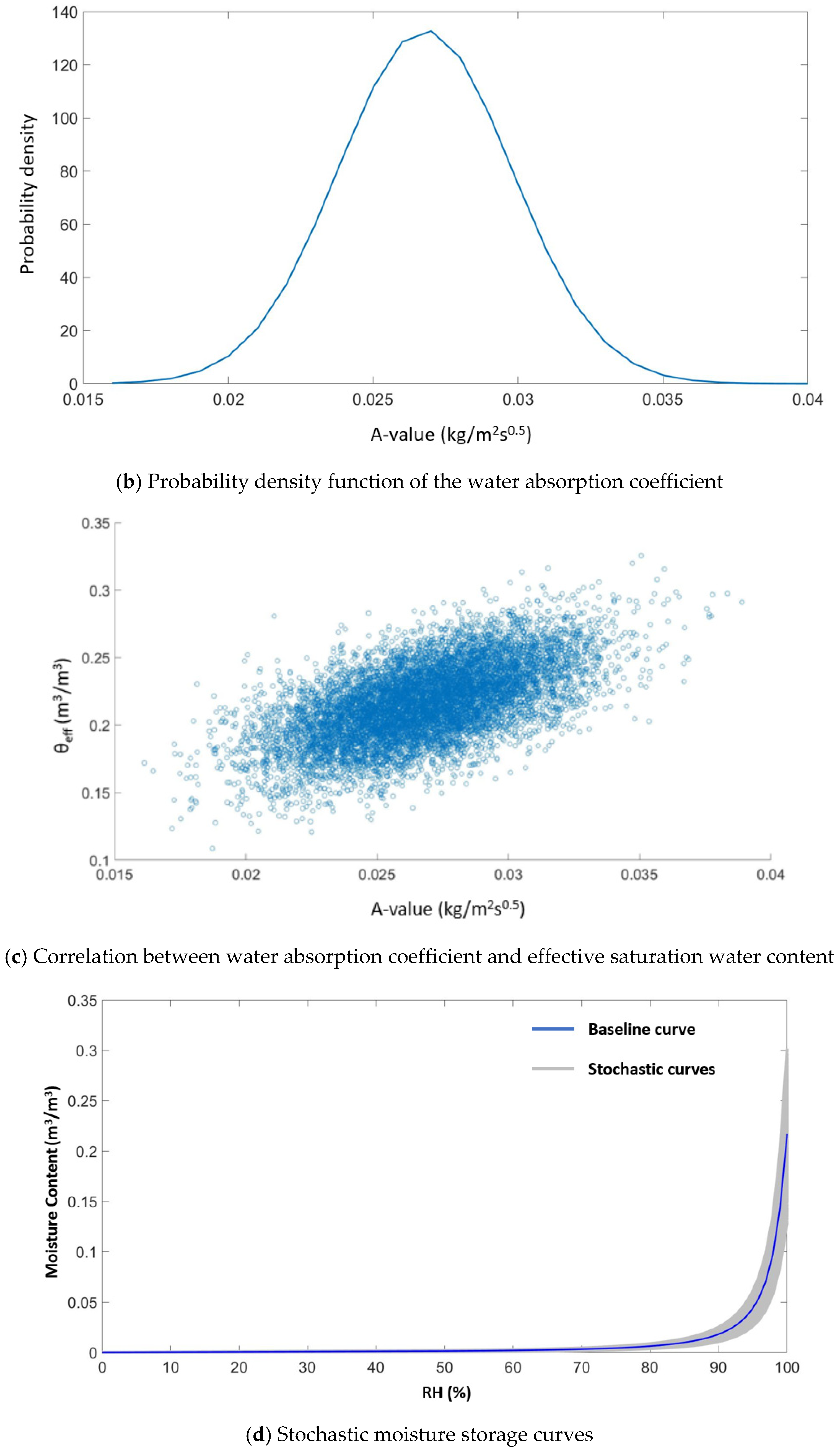
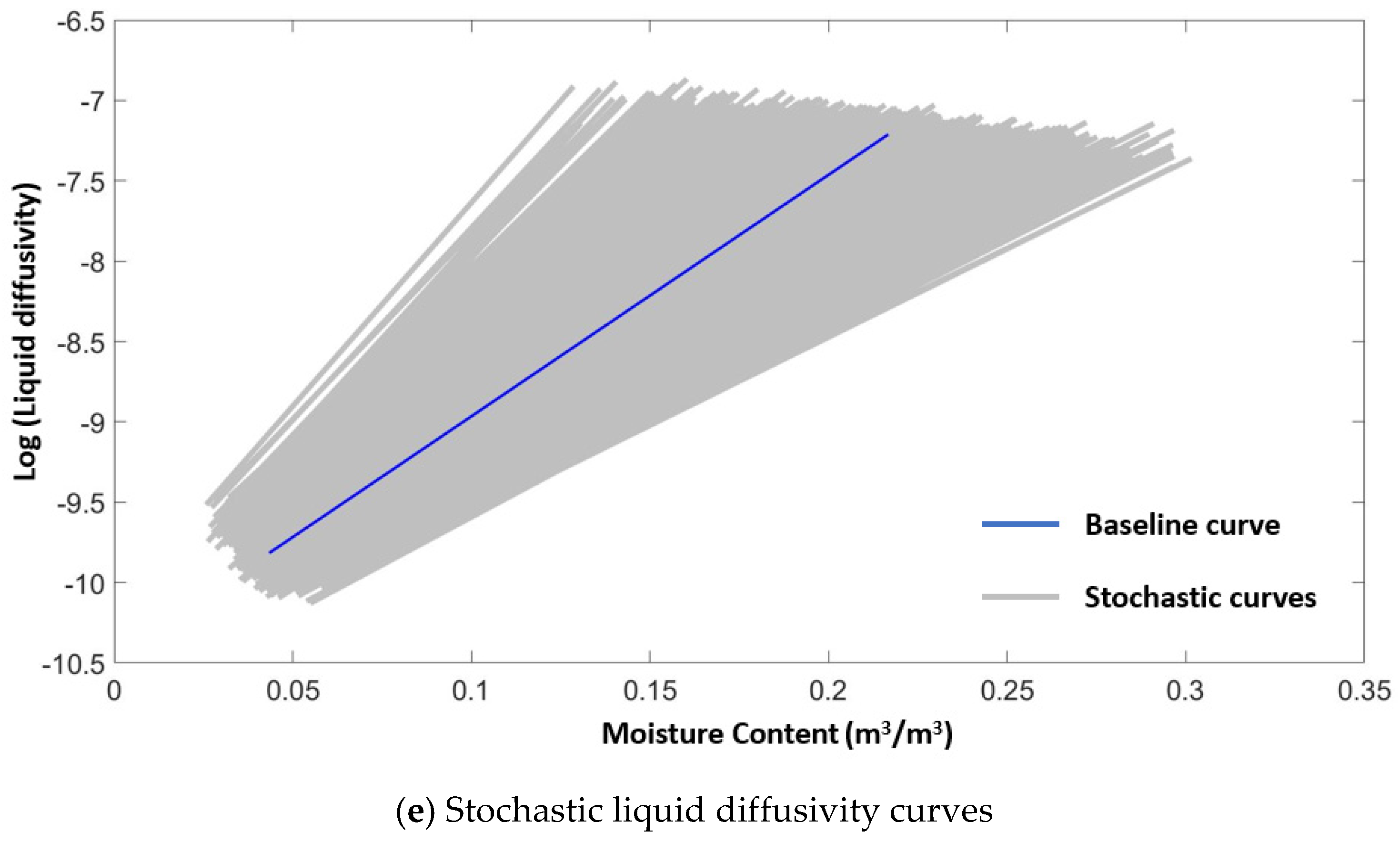
2.2.4. Brick Properties

As mentioned in Section 2.1.1, the water absorption coefficient (A-value) and effective saturation water content (θ_eff) of brick were considered as stochastic material properties. The material properties of red matt clay brick were used from a baseline model [32]. To quantify the range of these two brick properties, a literature review was conducted to determine the A-value and θ_eff of similar types of brick. A summary of these values is given in

Table 7. Literature review on A-value and effective saturation water content of brick.

Authors	Years	Name of Brick	Density (kg/m3)	A-Value (kg/m2s0.5)	θeff (m3/m3)
Kumaran et al. [32]	2002	Red matt clay brick	1935	0.0268	0.217 (Vacuum)
		Textured coated clay brick	1821	0.0322	0.333 (Vacuum)
Mensinga [53]	2009	Clay brick 1	2212	0.032	0.192 (5 h boiling) 0.228 (Vacuum)
		Clay brick 2	2223	0.028	0.182 (5 h boiling) 0.219 (Vacuum)
Zhao [54]	2012	Old building brick Dresden1	1948	0.0219	0.179 (Partially immersed in water for 2 weeks)
		Old building brick Dresden2	1736	0.034	0.32 (Partially immersed in water for 2 weeks)
Yousefi [55]	2019	Clay brick	2080	0.012	0.116 (Partially immersed in water for 8 days)
Aldabibi [56]	2020	Reclaimed exterior brick	1968	N/A	0.242 (5 h boiling)
		New exterior brick	1904	N/A	0.198 (5 h boiling)

. The effective saturation water content, θ_eff, is that of the maximum degree of saturation as may occur over the long-term immersion. However, the effective saturation water content is subject to a large uncertainty depending on different test methods used to assess this value, be this using the long-term with partial immersion in water, 5 h boiling saturation, or vacuum saturation test methods. According to Mensinga [53], the 5 h boiling saturation water content is about 20% lower than that obtained using vacuum saturation. Even using the same test method, the measurement uncertainty is quite high. For example, the vacuum saturation is largely dependent on the vacuum pressure applied to the specimen, and the uncertainty in applied vacuum pressure can result in ca. ±20% of uncertainty for the θ_eff from vacuum saturation [53]. Furthermore, the properties amongst different specimens in the same brick category have large uncertainties due to the manufacturing process. According to Kumaran [33], the uncertainty in the vacuum saturation water content amongst 9 brick specimens is about ±40%. Zhao [54] measured the effective saturation water content of 23 brick specimens within the same brick category through 2 weeks of partial immersion; it was found that the uncertainty can be as high as ±37%. By considering the values for the effective saturation water content of clay brick and the uncertainties reported from different literature, the range for the effective saturation water content within one type of brick was set as ±40%. A normal probability distribution was generated by assuming the mean value as 0.217 m³/m³, with a standard deviation of 0.043 m³/m³.

For the A-value, the normal probability distribution was generated by assuming the mean value as 0.0268 kg/m²s^0.5, and standard deviation as 0.005 kg/m²s^0.5; as such, the uncertainty also falls within ±40%. According to the statistical analysis of 23 brick specimens by Zhao et al. [57], the effective saturation water content is positively correlated with the A-value with a correlation coefficient of 0.6. For this paper, then, the probability distributions of effective saturation water content and A-value were assumed as positively correlated with a coefficient of 0.6. Figure 8 shows the probability density functions of the brick properties, the correlation between A-value and θ_eff, and the stochastic moisture storage curves, liquid diffusivity curves derived from stochastic A-value and θ_eff.

The stochastic θ_eff was used to scale the moisture storage curve, and the liquid diffusivity curve was calculated based the stochastic θ_eff and A-value through Equation (9) [58,59]:

$${\mathrm{D}}_{\mathrm{w} }={\left(\frac{\mathrm{A}}{{\mathsf{\theta }}_{\mathrm{eff}}}\right)}^2\times \frac{{\mathrm{b}}^2}{2\mathrm{b}-1}\times \exp \left(\mathrm{b}\times \left(\frac{\mathsf{\theta }}{{\mathsf{\theta }}_{\mathrm{eff}}}-1\right)\right)$$

(9)

where

• D_w—liquid diffusivity at unsaturated water content, m²/s
• θ_eff—effective saturation water content, kg/m³, 10³ ∙ m³/m³
• θ—unsaturated water content, kg/m³, 10³ ∙ m³/m³
• A—water absorption coefficient, kg/m²s^0.5
• b—shape factor, determines the slope of the liquid diffusivity curve; value can be between 5 and 10; In this paper, b was assumed as 7.5.

In fact, the variation of the value of b from 5 to 10 will result in considerable uncertainty in the simulation results although the value of b can be determined based on a wetting and drying test; however, this was beyond the scope of the work reported in this paper. What should be noted is that different researchers hold different opinions on which saturation water content should be used for deriving the liquid diffusivity. Kunzel [60] suggested the use of the free water saturation, which is the maximum moisture content achieved in a water uptake experiment, the free water saturation water content corresponds to the capillary saturation water content in Delphin [31]. Carmeliet et al. [61] have a similar opinion to that of Kunzel, given that water absorption at a moisture content level above capillary saturation is dominated by the diffusion of entrapped air. In this instance, the relationship between liquid diffusivity and moisture content in the capillary range is not applicable in the “over-capillary” range. Kumaran [58] used vacuum saturation water content to estimate the averaged liquid diffusivity in capillary and over-capillary ranges of spruce, and the estimated liquid diffusivity was in the same order of magnitude as the measured liquid diffusivity. In Delphin, the effective saturation water content is used to scale the moisture storage curve and liquid diffusivity curve when the measured sorption and liquid diffusivity curves are not available, whereas, the capillary saturation water content is not used in hygrothermal simulations [31]. Therefore, in this paper, the effective saturation water content was used to derive the liquid diffusivity curve. In fact, the stochastic effective saturation water content takes into consideration the measurement uncertainty as well as the uncertainty amongst different specimens within the same category. Therefore, it also covers the possible range of values for effective saturation water content from capillary saturation to vacuum saturation.

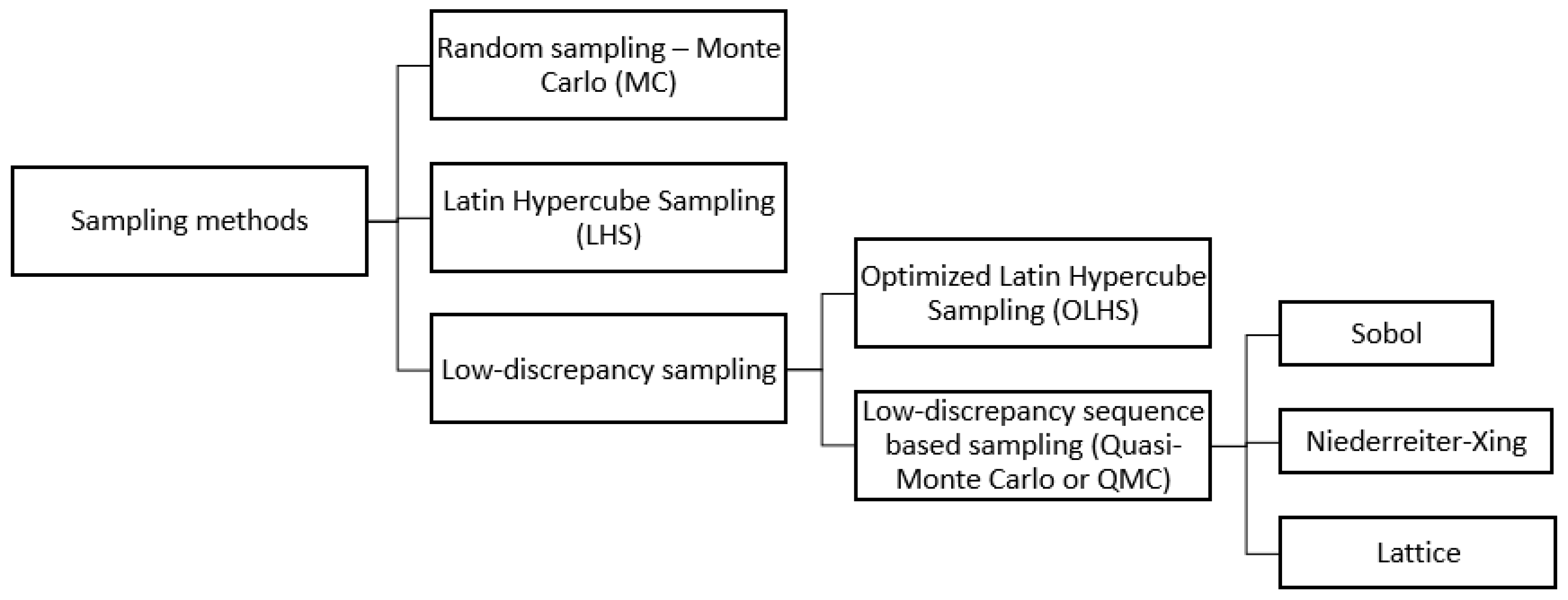
2.3. Literature Review of Sampling Methods

The sampling method used for stochastic simulation largely determines the efficiency and reliability of the stochastic simulation. The purpose of sampling design is to improve the sampling efficiency, which can be described as the sample size required to achieve results having an acceptable level of accuracy.

Table 8. Literature review on sampling methods.

Authors	Year	Simulation Objects	Sampling Methods	Number of Stochastic Variables	Sample Size	Convergence Size
Lomas and Eppel [64]	1992	Whole building energy model	Random	70	100	100
Salonvaara et al. [17]	2001	Hygrothermal model	Random	16	100	N/A
Hyun et al. [65]	2007	A building ventilation model	Latin Hypercube	13	30	N/A
Macdonald [66]	2009	Infiltration rate as a function of temperature & wind speed	Random; Stratified; Latin Hypercube	2	100; repeated 100 times	100 for all three sampling methods
Zhao et al. [18]	2011	Hygrothermal model	Random	36	400	N/A
Burhenne et al. [62]	2011	Whole building energy model	Random; Latin Hypercube; Stratified sampling; Sobol sequence-based sampling	4	16, 32, 64, 128, 256, 512; each size repeated 100 times	Random sampling: 256; Other: 64
Defraeye et al. [67]	2013	Hygrothermal model	Random	6	2000	N/A
Janssen [63]	2013	Hygrothermal model	Random; Optimized Latin Hypercube (OLHS)	4	10, 20, 50, 100, 250, 500; each size repeated 10 times	OLHS converged faster than random
Goffart et al. [68]	2015	Whole building energy model	Latin Hypercube	14	600	400
Hou et al. [29]	2019	Hygrothermal model	Random; OLHS; Sobol; Neiderreiter-Xing; lattice sequence	7	80, 160, 320, 640, 1280	QMC converged faster than MC for smooth objective functions
Bui et al. [69]	2020	Hygrothermal model	Latin Hypercube	5	1000	600

lists sampling methods used for stochastic simulation of building energy or hygrothermal performance, as well as the number of stochastic variables and sample size in previous studies. Figure 9 illustrates the categorisation of different sampling methods listed in Table 8. It can be seen that the sample size used for stochastic simulation varies from several hundreds to a few thousands. Among the studies listed in Table 8, in references [29,62,63] the random sampling methods (Monte Carlo: MC) have been compared with methods for low discrepancy sampling (Quasi-Monte Carlo: QMC or Optimized Latin Hypercube Sampling: OLHS). They all concluded that low-discrepancy sampling offered a higher sampling efficiency than MC methods in many circumstances. As to the comparison between different low-discrepancy sampling methods, both references [29,62] suggest QMC based sampling performs better than either the Replicated Latin Hypercube Sampling (RLHS) or Optimized Latin Hypercube Sampling (OLHS) methods. In reference [62], Burhenne et al. compared 100 sets of 256-run simulations using Latin Hypercube Sampling with 100 sets of Sobol sequence-based sampling (one of the QMC methods). It was found that the sampling based on the Sobol sequence had less variation in the 100 CDFs than the Latin Hypercube Sampling method. Hou et al. [29] found a better performance for QMC than for MC when predicting heat loss of a masonry wall assembly, however, the superiority of QMC over MC becomes less significant when predicting freeze/thaw cycling because the number of dominant stochastic variables in respect to freeze/thaw cycling is more than that for heat loss. In a situation where the number of dominant stochastic variables is not known, the performance of the QMC method will be better than or equal to the MC method. Therefore, in this paper, the Sobol sequence-based sampling was used to sample the stochastic discrete and continuous variables, as this sampling method allows a robust and conservative error estimation.

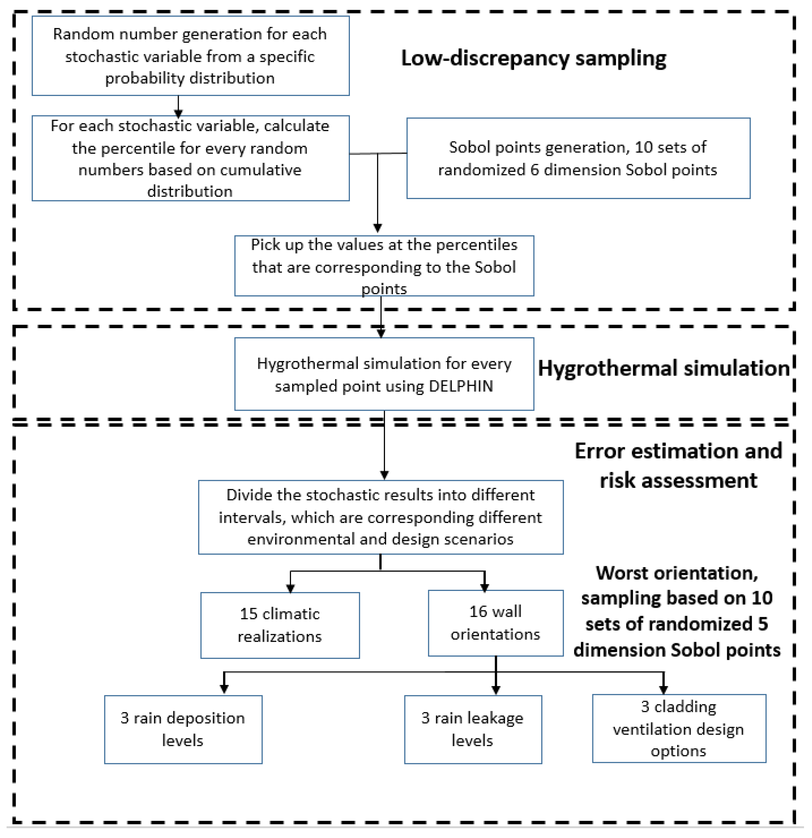
2.4. Implementation of Sobol Sequence-Based Sampling

To implement the Sobol sequence-based sampling, 10 sets of 6-dimensional randomised Sobol sequences were generated, the randomisation was based on the scramble approach [70]. For continuous stochastic variables, they were mapped into the space of [0, 1] through their cumulative distribution, and the values at the percentiles which corresponds to the Sobol points were then selected. For discrete variables, i.e., the climatic realisations, the space of [0, 1] was divided into 15 equal intervals, i.e., [0, 1/15], [1/15, 2/15], ……, [14/15, 15/15]. When the Sobol point falls into the first interval, then the first realisation (R01) will be selected; similarly, when the point falls into the second interval, R02 will be selected, and so on.

For the rain leakage moisture source and cladding ventilation rate, there were three levels selected, with each level having a specific cumulative distribution. To guarantee that the cumulative distribution at each level is unchanged and the sample sizes at different intervals are equal, the space of [0, 1] was divided into three intervals: [0, 1/3], [1/3, 2/3] and [2/3, 1]. When the Sobol point falls into the first interval, then the low level will be selected, and the stochastic values at that level will be selected by mapping the percentiles in the cumulative distribution to the interval of [0, 1/3]. Similarly, the values in the middle level and high level were also selected in the same way.

For the rain deposition factor, this was assumed to be uniformly distributed through 0.35 to 1; therefore, it was directly mapped to Sobol points through a uniform cumulative distribution with the sampled values at each category of rain deposition factor being also uniformly distributed. Similarly, the orientation was also assumed as a uniform distribution, and divided into 16 equal intervals, and each interval is 22.5°, for example, 11.25° to 33.75° represents NNE, 33.75° to 56.25° represents NE and so on. For North orientation, it includes two sub-intervals with each has 11.25°: 348.75° to 360° and 0° to 11.25°.

Although there were 7 stochastic variables, the A-value and effective saturation water content of brick were positively correlated with a correlation coefficient of 0.6; using two columns of Sobol points to sample these two parameters would disrupt their correlation. Therefore, the water penetration coefficient, which is defined as the ratio of A-value to saturation water content [60], was used to map Sobol points. In this way, the two stochastic brick properties can be sampled by one column of Sobol points, and their correlation can be retained. In

Table 9. Stochastic variables.

Variables	Distribution	Range	Intervals
Climatic realisation	Discrete	R01–R15	-
Orientation	Uniform	0–360	16 Orientations, interval of N 348.75~11.25, NNE 11.25~33.75 and so on…
Rain deposition factor	Uniform	0.35–1;	Low 0.35~0.56; Middle 0.56~0.78; High 0.78~1.
Rain leakage moisture source (% of wind-driven rain)	Normal	0–2.0	Low 0.3 (0.35); Middle 0.56 (0.35); High 0.8 (0.35)
Cladding ventilation rate (ACH)	Normal	1–20	Low 3 (0.67); Middle 5.5 (1.4); High 10.5 (3.5)
Water absorption coefficient (A-value) of brick (kg/m2·s0.5)	Normal	0.0161–0.0389	0.0268 (0.005)
Effective saturation water content of brick (m3/m3)	Normal	0.108–0.325	0.217 (0.043)

Note: For the variables having normal distribution, the values in the parenthesis are standard deviations. The distributions of rain leakage moisture source are truncated above zero; the distributions of cladding ventilation rate are truncated above 1.

, a summary is given of the different stochastic variables, their ranges as well as their respective distributions.

What should be noted is that the rain leakage moisture source and cladding ventilation rate are dependent on micro-climatic conditions. Ideally, the climate-dependent time series of these two variables can be used for hygrothermal simulation. However, in this study, every stochastic value for the moisture source or ACH was assigned to a single stochastic model, meaning that every single stochastic model has a constant moisture source or ACH through a 2 year simulation period. The variations of the stochastic variables are reflected from different stochastic models having different constant values of moisture source and ACH.

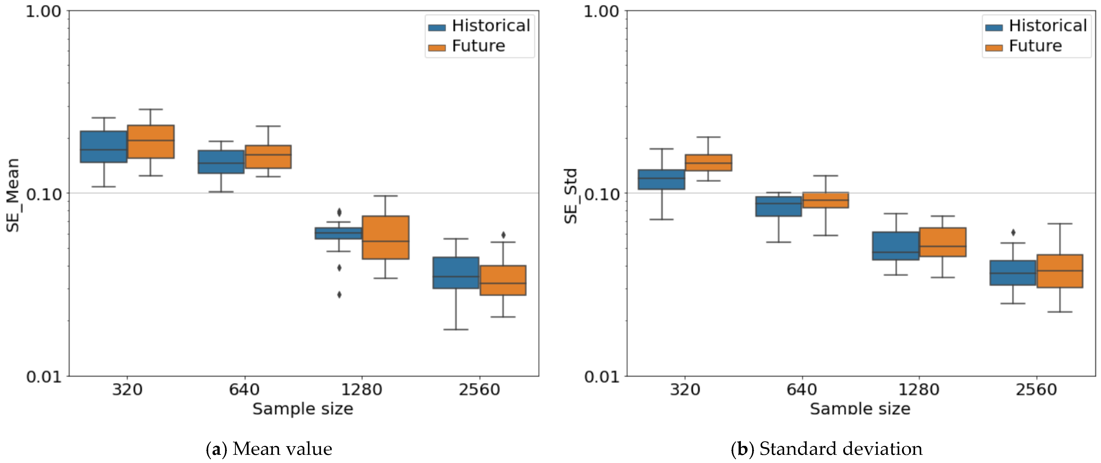
2.5. Error Estimation and Risk Assessment

The mould growth index was calculated based on the use of the VTT model with a decline factor of 0.3 [71]. The relative humidity and temperature of the exterior surface of OSB were extracted for calculating the mould growth index. The averaged values for mould growth indices over two years were calculated for error estimation and mould growth risk assessment. The values for standard error of the mean and standard deviation were calculated based on Equations (10) and (11), respectively [29]:

$${\overline{Q}}_{n,r}\left(f\right)=\frac{1}{r}{\displaystyle \sum }_{i=1}^r{Q}_n^{\left(i\right)}\left(f\right)$$

(10)

$$stderr\left({\overline{Q}}_{n,r}\right)=\sqrt{\frac{1}{r\left(r-1\right)} {\displaystyle \sum }_{i=1}^r{\left(Q_n^{\left(i\right)}\left(f\right)-{\overline{Q}}_{n,r}\left(f\right)\right)}^2}$$

(11)

where:

• $Q_n^{\left(i\right)}\left(f\right)$—the estimator of mean or standard deviation of the ith randomised sequence
• ${\overline{Q}}_{n,r}\left(f\right)$—the average of the estimators of r sets of randomised sequences
• r—the number of randomised sequences; in this paper, r is 10

The error estimation was performed for the whole sample space and the sub-spaces for different climatic realisations and orientations at different sample sizes. In this paper, the error estimation for the whole sample space was performed at sizes of 2³ × 10, 2⁴ × 10 up to 2⁸ × 10. For the sub-spaces, the error estimation started from a sample size of 2⁵ × 10 ended up with 2⁸ × 10, as the sample size of each sub-space is approximately the total sample size divided by the number of intervals. The maximum sample size was determined by considering the balance between the computational cost and the accuracy of the results. For the whole sample space, the sample size of 2⁸ × 10 gave a standard error in the magnitude of 10⁻³, whilst, for each sub-space, the sample size of 2⁸ × 10 gave a standard error in the magnitude of 10⁻². According to Hou et al. [29], the standard errors calculated from Equations (10) and (11) is roughly in the same order of magnitude as the absolute error that was obtained by comparing the results at different sample sizes (2³ × 10, 2⁴ × 10 up to 2⁷ × 10) with a very large reference sample size—40,960. The results of standard error were discussed in Section 3.1 and Section 3.2. Then the mould growth risk for different climatic realisations and orientations were assessed based on the results from the highest sample size.

To investigate the effect of mould growth risk mitigation strategies, the orientation that has the highest mean value for the 2-year mould growth index was selected for further stochastic simulation. Thereafter, the mould growth risk was assessed for different levels of rain deposition factors, rain leakage moisture sources, and cladding ventilation rates for the worst orientation. Figure 10 shows the overall procedure for low-discrepancy sampling, stochastic simulation, error estimation and risk assessment.

3. Results and Discussion

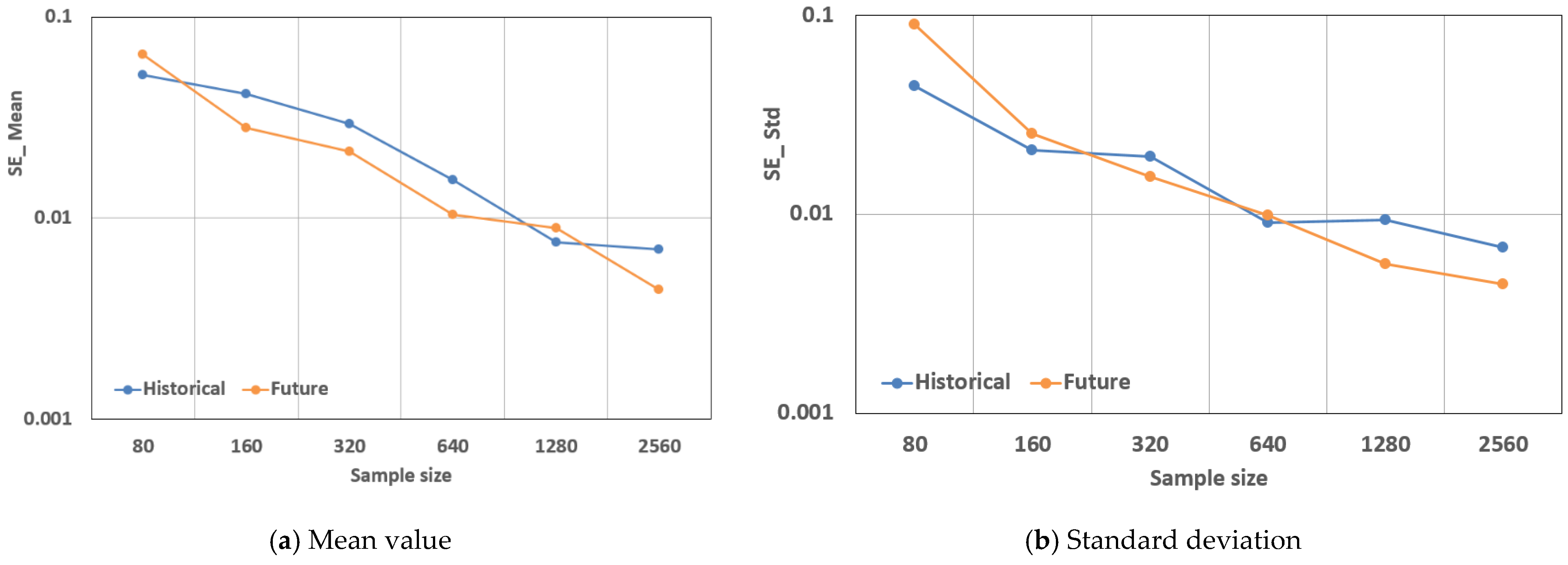
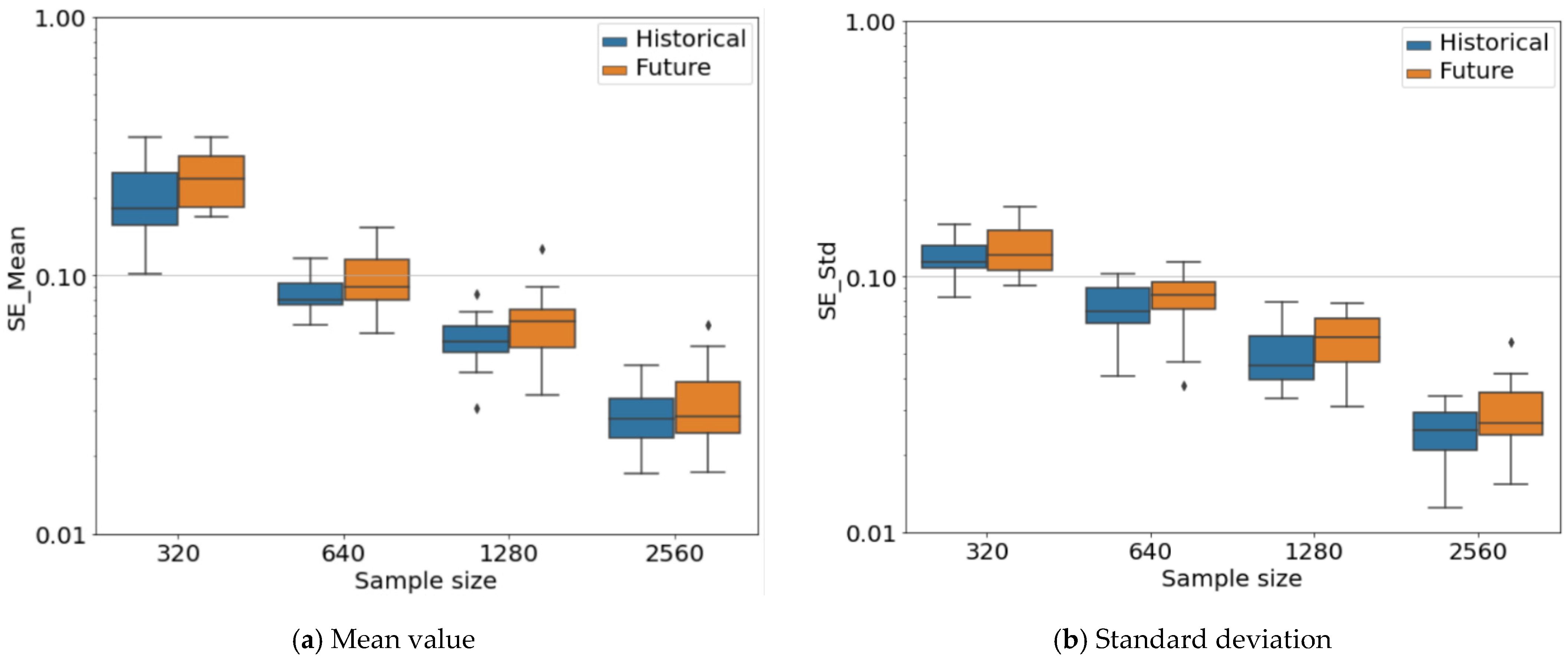
3.1. The Whole Sample Space

Figure 11 shows the standard error of the mean value and standard deviation of the 2-year averaged mould growth index at different sample sizes of the whole sample space, which means all the climatic realisations and orientations, as well as other stochastic variables, were taken into account. It can be seen that the standard errors generally decrease with an increase in sample size, although the decreasing rates are different at different sample size intervals, i.e., for the mean value of the historical period, the decreasing rate is greater from 320 to 1280 than from 80 to 320. When the sample size is increased to 1280-run, the standard error can be reduced to the magnitude of 10⁻³ for both historical and future periods. As shown in

Table 10. Mean value and standard deviation of 2-year averaged mould index at a 2560-run.

	Historical Period	Future Period
Mean value	1.06 1 SE 0.007	1.44 SE 0.004
Standard deviation	0.91 SE 0.007	1.08 SE 0.004

¹ SE: standard error.

, the future period has a higher mould growth index than the historical period, but the standard deviation in the future is very similar to that in the historical period. The standard error in the future period is slightly lower than that in the historical period. The mould growth index listed in Table 10 reflects the overall mould growth risk in the city of Ottawa, with all the climatic realisations, orientations and other stochastic variables taken into account.

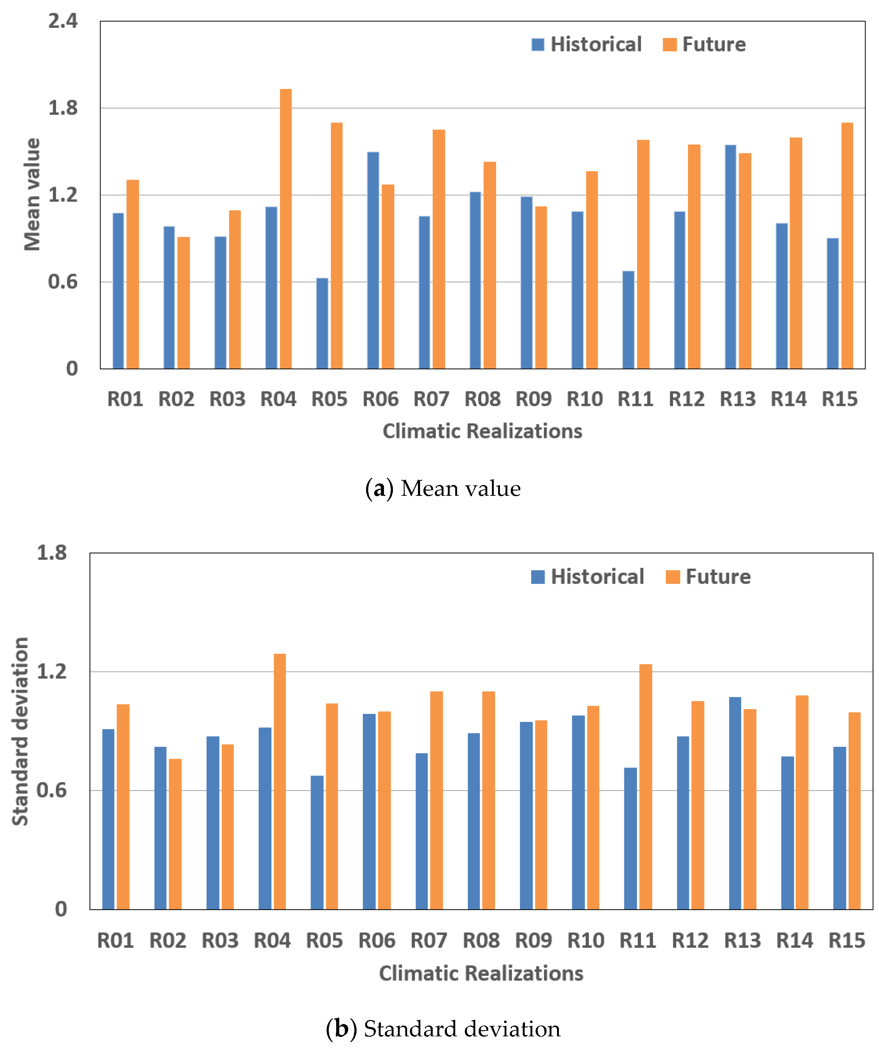
3.2. Different Climatic Realisations

Figure 12 shows the standard errors at different sample sizes for different climatic realisations of historical and future periods. Each box represents the standard errors of 15 climatic realisations in a climatological period. In general, the standard errors for different climatic realisations are higher than those for the whole sample space, since the sample size for each climatic realisation is roughly equal to the total sample size divided by 15. It can be seen that there is a significant variation of the standard error for different climatic realisations, and the standard errors for the future period are generally higher than those for the historical period. The standard errors of mean values and standard deviation values can be reduced to the magnitude of 10⁻² after 1280 runs, except for the mean values of the future period, which needs 2560 runs to ensure all the standard errors fall into the magnitude of 10⁻².

Figure 13 shows the mean value and standard deviation of the 2-year averaged mould growth index for historical and future periods using 2560-run for which the standard error for each climatic realisation is in the magnitude of 10⁻². It can be seen that most of the climatic realisations have a higher mould growth index in the future than in the historical period. The future period also has a higher variability in the mould growth index than the historical period given the higher standard deviation. The variation in mould growth index among different climatic realisations is more significant than the variation in moisture index as shown in Figure 2. As shown in Figure 14a,b, there is no clear relationship between mould growth index and moisture index based on the stochastic simulation results when all the orientations were taken into account. However, the significance of the relationship was increased when the analysis only focused on the orientation that receives the highest amount of WDR (The sample size was locally expanded for the worst orientation to guarantee the standard errors were in an order of magnitude of 10⁻²).

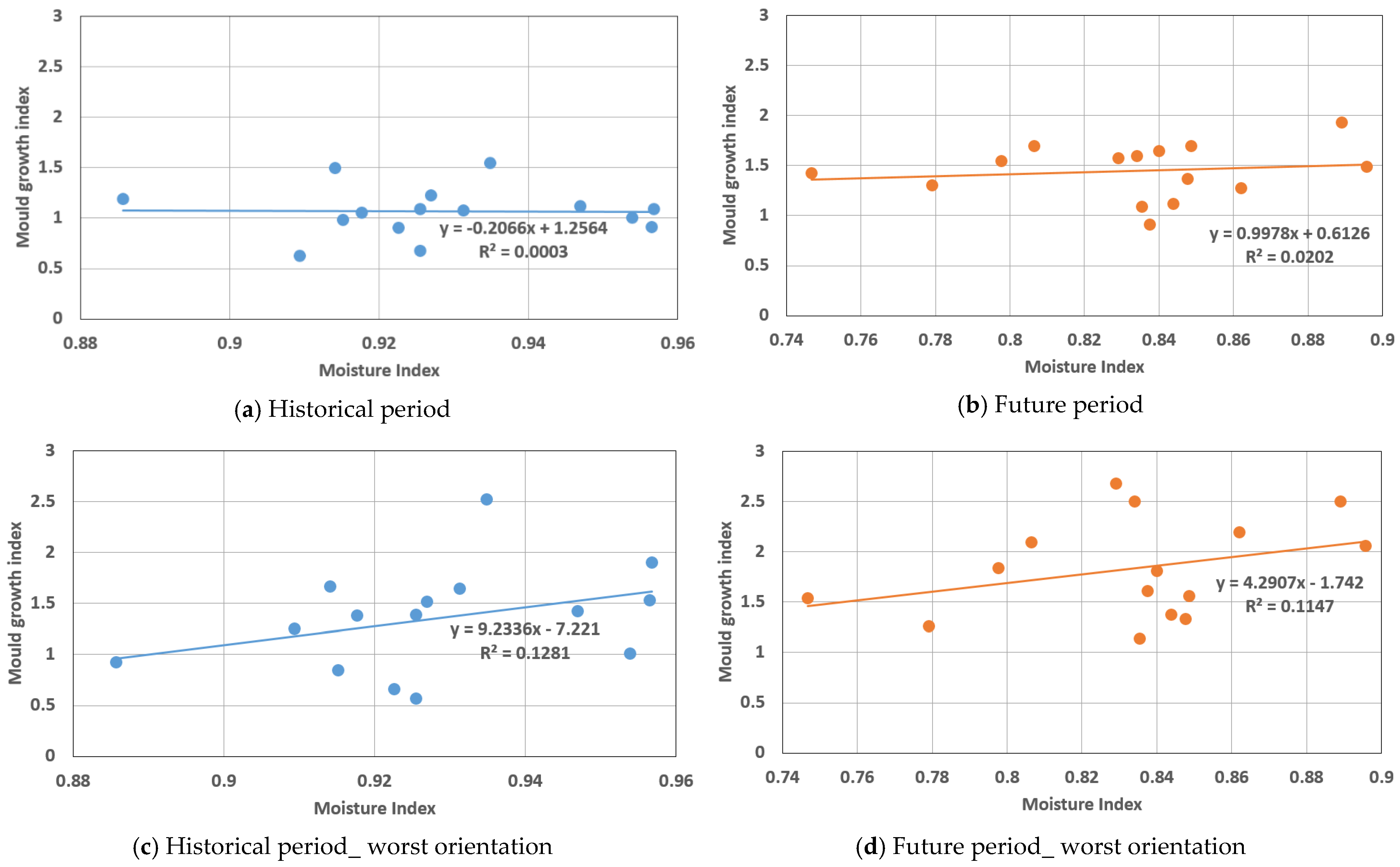
3.3. Different Orientations

Figure 15 shows the standard errors of the mean value and standard deviation of different orientations for historical and future periods (Each box represents the standard errors for 16 orientations at each climatological period). It can be seen that the decreasing rates of the standard errors for different orientations are lower than those for different climatic realisations, particularly from 320-run to 640-run, and future period generally has higher standard errors than historical period. The variation of standard error among different orientations is significant; for example, the north orientation has a standard error of mean value close to 0.1 with 320 runs, but the standard error for south orientation cannot be reduced to below 0.1 until 1280 runs. The standard errors of all the orientations can be reduced to the magnitude of 10⁻² after 1280 runs, which means for each orientation 80 runs can achieve a standard error lower than 0.1.

Figure 16 shows the mean value and standard deviation of the 2-year averaged mould growth index for different orientations using 2560 runs, which has a standard error of around 0.05 for all orientations. It can be seen that the mean value and standard deviation of the mould growth index for the future period are higher than those for the historical period for all orientations. The orientation that had the highest mean value of mould growth index was SSW, which is the same orientation that had the highest amount of wind-driven rain (Figure 3). The orientation that has the highest standard deviation of mould growth index (SSW) is different from that having the highest standard deviation of wind-driven rain (N for historical, NW for future, Figure 3), this might be caused by the influence of solar radiation.

The SSW orientation was selected as the orientation for further stochastic simulations and the one providing the most severe conditions to which to subject wall assemblies when investigating the mould growth risk under different mitigation strategies.

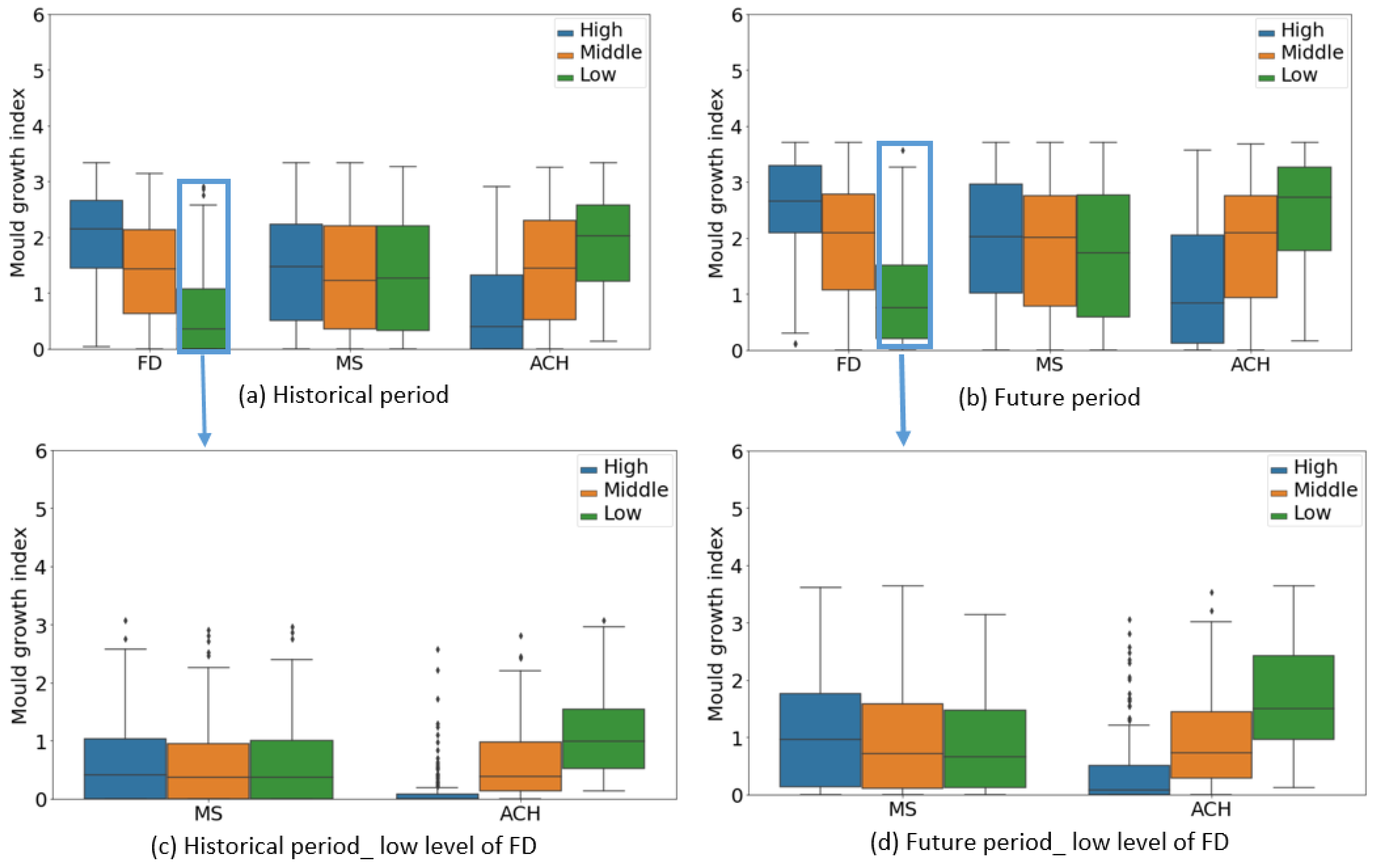
3.4. Different Mould Growth Risk Mitigation Strategies

To investigate different mould growth risk mitigation strategies, an additional 640-run stochastic simulations were performed for the worst orientation selected in Section 3.3. Figure 17 shows the stochastic 2-year averaged mould growth index within different levels of control for different mould growth risk variables, i.e., the rain deposition factor, rain leakage moisture source and cladding ventilation rate as described in Table 9. Each box represents the stochastic 2-year averaged mould growth index of one level of a specific mould control variable with all the other stochastic variables varying in their full range of values. For example, the green box in the case of F_D represents the low level of rain deposition factor (0.35~0.56) with all the other stochastic variables (climatic realisations, rain leakage moisture source, cladding ventilation rate, and brick properties) varying in their full range of values. As such, if the mould growth index can nonetheless be reduced by controlling one specific variable in consideration of all the uncertainties, the influence of this variable can be considered as a robust control strategy. The 640-run stochastic simulation based on RQMC gave the standard error of mean value and standard deviation of mould index for each level of each risk control variable of ca. 0.05.

3.4.1. The Influence of Rain Deposition Factor and Cladding Ventilation Rate

In Figure 17, it can be seen that the reduction of the rain deposition factor and increase of ventilation rate can significantly reduce the mould growth index, and the uncertainty at a low level of rain deposition factor is lower than that at the high level of cladding ventilation rate, particularly in the future period. This indicates that, under the climatic conditions of Ottawa, controlling the rain deposition factor could be a more robust mitigation strategy than increasing the cladding ventilation rate. The same stochastic simulations were also implemented for Halifax, a coastal city in Canada. It was found that ACH plays a more important role in controlling mould growth than the rain deposition factor. Therefore, the most robust design or risk mitigation strategy varies depending on the climatic zone.

As was discussed in Section 2.2.1, a 0.1-m overhang can achieve, in the historical period, a low-level rain deposition factor, which can reduce the 75 percentile mould growth index to below 1, and 1.5 for the future period. On the other hand, the highest level of the cladding ventilation rate (ventilated cavity with 4 openings as calculated in Section 2.2.3) can, for the historical period, reduce the 75 percentile mould growth index to below 1.2 and for the future period to a value below 2. Since the 0.1-m overhang is the most robust strategy in controlling mould growth, further simulations were performed for a 0.1-m overhang with different levels of moisture source and ACH, for which the results are presented in Figure 17c,d. It can be seen that for a building with a 0.1-m overhang and a ventilation design having 4 openings, the mould growth index can be controlled within the value of 1 for most of the stochastic cases in both historical and future climate periods, although the mould growth index is higher in the future period than in historical period.

3.4.2. The Influence of Rain Leakage Moisture Source

There is no significant difference between different levels of rain leakage moisture source, although the mould growth index for the low level of MS is slightly lower than that for the middle and high levels of MS (Figure 17). This is because of the protection provided by the water-resistive barrier. However, the uncertainty within each level of MS is very high (Figure 17a,b), and the uncertainty was caused by other stochastic variables, i.e., rain deposition factor, ACH, climatic realisations and brick properties. The uncertainties were reduced within the low level of rain deposition factor (Figure 17c,d).

The rain leakage modelling approach was based on ASHRAE 160, which assumes the moisture source on the exterior surface of the sheathing membrane. However, the rainwater may penetrate through the sheathing membrane and reach the OSB sheathing if there was a defect in the sheathing membrane. To consider this situation, an additional set of simulations was performed with the moisture source assigned to the exterior layer of OSB, which represent a higher mould growth risk scenario than the moisture source assigned to the sheathing membrane for the future period (Figure 18a). As opposed to the high-risk scenario, for comparison, another scenario without any rain leakage was simulated based on the future period (Figure 18b).

When the moisture source was deposited on the exterior layer of the OSB (Figure 18a), the difference between different levels of moisture source is more significant than the scenario with the moisture source deposited on the exterior surface of the sheathing membrane (Figure 17b). The overall mould growth indices increased for the low level of rain deposition factor and high level of cladding ventilation rate, whilst, the increase in the low level of rain deposition factor is lower than that in the high level of cladding ventilation rate, i.e., the 75 percentile mould growth index at a low level of F_D increased from 1.5 to 1.8, and that at the high level of ACH increased from 2.0 to 2.7. (e.g., compare results given in Figure 17b to those in Figure 18a).

For the scenario without moisture source, the overall mould growth indices at different levels of F_D and ACH were reduced (Figure 18b). The 75 percentile mould growth index at a low level of FD decreased from 1.5 to 1, and that for a high level of ACH decreased from 2 to 1.5 (Figure 17b compare to Figure 18b). Therefore, it can be said that improvements in water tightness can reduce mould growth risk overall.

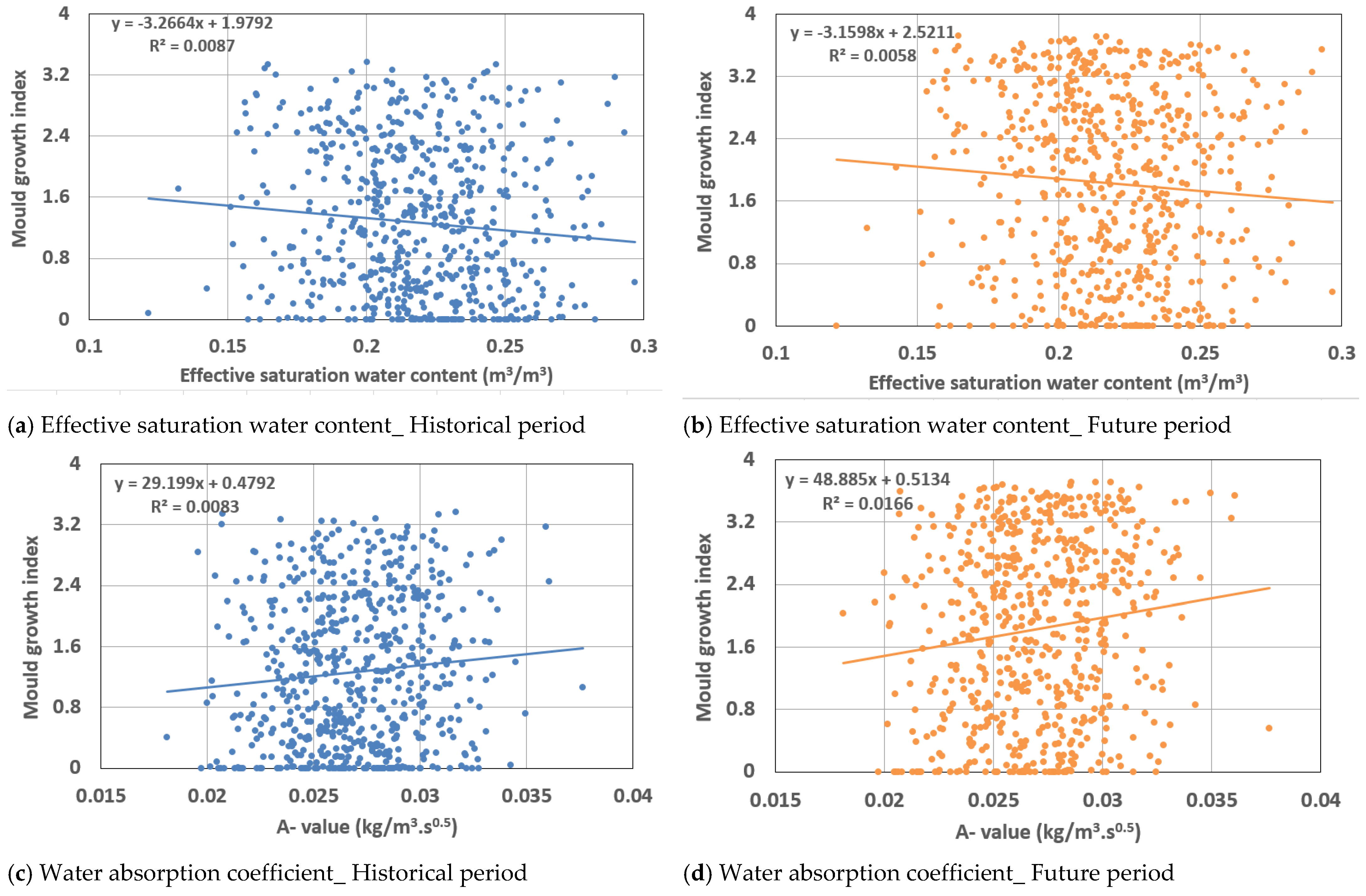
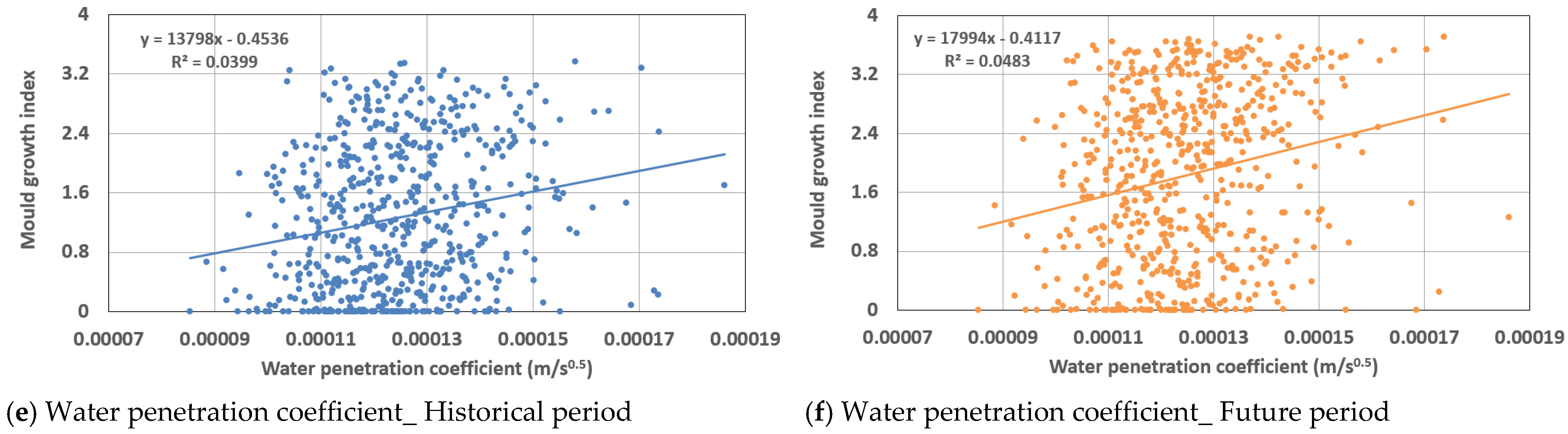
3.5. The Influence of Brick Properties

Figure 19 shows the scatter plots of the 2-year averaged mould growth index against the brick properties. These plots are based on 640 runs using the most severe climate load orientation (SSW), and the presence of a rain leakage moisture source on the sheathing membrane. Both decreasing and increasing trends in mould growth index can be observed, although the linear relationship between mould growth index and the brick properties is very weak due to the disruption of other influential stochastic variables. Generally, the mould growth index slightly decreases with an increase in the effective saturation water content, and it increases with an increase of the water absorption coefficient (A-value) and water penetration coefficient, the increasing trend being more significant for the water penetration coefficient. For the effective saturation water content, there is no significant difference in the decreasing rate between historical and future periods. For the A-value and water penetration coefficient, the increasing trend is more significant for the future period than the historical period, and the R² value for the water penetration coefficient is higher than that for A-value. Although the A-value and effective saturation water content are the two properties that are measured from laboratory tests, the water penetration coefficient, i.e., the ratio of A-value to effective saturation content, is a more useful parameter in reflecting the water penetration capability of brick and assessing the influence on mould growth performance of the wood sheathing in wood-frame wall assemblies.

4. Conclusions

The use of a stochastic approach has been applied for assessing building performance from simulations now for a few decades, and it continues to show its usefulness in uncertainty analysis and risk assessment given increasing in computational capacity, particularly in the current setting where climate change brings more uncertainties to results from hygrothermal simulation. The results described in this paper have demonstrated the use of a stochastic hygrothermal simulation procedure to evaluate the mould growth risk of a wood-frame building envelope, considering various uncertainties such as climate realisations, wall orientations, material properties and the stochastic variables related to risk mitigation strategies that included: rain deposition factor, rain leakage moisture source and cladding ventilation rate. The stochastic simulation was based on the historical and future climatic conditions of Ottawa, a Canadian city located in a cold climate zone. A randomised Sobol sequence-based sampling, one of the Randomized Quasi-Monte Carlo (RQMC) methods, was used for sampling the stochastic variables, and error estimation was conducted for different climatic realisations and wall orientations at different sample sizes. The main conclusions were:

There were large variations in standard error among different climatic realisations and different wall orientations at the same sample size, nevertheless, the standard error can be reduced to the magnitude of 10⁻² after 1280-runs for all 15 climatic realisations and 16 wall orientations, which indicates for each climatic realisation or wall orientation, the standard error can be controlled at the magnitude of 10⁻² after 80-runs.

The mould growth rose map obtained from stochastic simulation has a similar shape to the wind-driven rain rose map obtained from the ASHRAE wind-driven rain model, which indicates that wind-driven rain might be a dominant parameter that influences mould growth in wall assemblies subjected to WDR. However, the mould growth index level of the 15 climatic realisations cannot be reflected by the moisture index level of the 15 climatic realisations due to the disruptive effects of other stochastic variables.

For the wall having red matt clay brick as cladding with material properties assumed in this paper, under climatic conditions of Ottawa, the deflection of wind-driven rain is the most robust mould growth risk control strategy as compared to improving the water tightness or improving cladding ventilation, particularly in future periods. The reduction of wind-driven rain can reduce both the rainwater absorbed by the brick and that penetrates the wall assembly. Improving water tightness can reduce overall mould growth risk at different levels of rain deposition factor and cladding ventilation rate.

With the same cladding and climatic conditions stated above, improving cladding ventilation will significantly reduce the overall mould growth risk, however, the uncertainty at a high cladding ventilation level (4-opening ventilated design) is higher than that at the low level of rain deposition factor (0.1 m overhang protection or steep-slope roof design), and the uncertainty is more significant in the future period.

Although the relationship between the brick properties and the mould growth index is very weak due to the interference of other stochastic variables, the decreasing trend of mould growth index was observed with the increase of effective saturation water content, whilst, the increasing trend was found with the increase of water absorption coefficient and water penetration coefficient, and the trend is more significant for the water penetration coefficient, particularly for the future period. The influence of the water penetration coefficient, which is defined as the ratio of A-value and effective saturation water content, is more significant than that of A-value and effective saturation water content.

References

1. Pachauri, R.; Meyer, L. Climate Change 2014: Synthesis Report. Contribution of Working Groups I, II and III to Fifth Assessment Report of the Intergovernmental Panel on Climate Change; IPCC: Geneva, Switzerland, 2014. [Google Scholar]
2. Zhang, X.; Flato, G.; Kirchmeirer-Yong, M.; Vincent, L.; Wan, H.; Wang, X.; Rong, R.; Fyfe, J.; Li, G.; Kharin, V.V. Changes in Temperature and Precipitation Across Canada. In Canada’s Changing Climate Report; Bush, E., Lemmen, D.S., Eds.; Government of Canada: Ottawa, ON, Canada, 2019; pp. 112–193. [Google Scholar]
3. Ali, S. Impact of Future Climate Change on the Building Performance of a Typical Canadian Single-Family House Retrofitted to the Passivehaus. Master’s Thesis, Concordia University, Montreal, QC, Canada, 2015. [Google Scholar]
4. Nik, V.M.; Kalagasidis, A.S.; Kjellstrom, E. Assessment of hygrothermal performance and mould growth risk in ventilated attic in respect to possible climate change in Sweden. Build. Environ. 2012, 55, 96–109. [Google Scholar] [CrossRef]
5. Defo, M.; Lacasse, M.A. Effects of Climate Change on the Moisture Performance of Tallwood Building Envleope. Buildings 2021, 11, 35. [Google Scholar] [CrossRef]
6. Hazleden, D.G.; Morris, P.I. Designing for durable wood construction: The 4 DS. In Durability of Building Materials and Components 8; Lacasse, M.A., Vanier, D.J., Eds.; National Research Council Canada: Ottawa, ON, Canada, 1999. [Google Scholar]
7. Foroushani, S.S.M.; Ge, H.; Nayler, D. Effect of roof overhangs on wind-driven rain wetting of a low-rise cubic building: A numerical study. J. Wind. Eng. Ind. Aerod. 2014, 125, 38–51. [Google Scholar] [CrossRef]
8. Ge, H.; Chiu, V.; Sathopoulos, T. Effect of overhang on wind-driven rain wetting of facades on a mid-rise building: Field measurements. Build. Environ. 2017, 118, 234–250. [Google Scholar] [CrossRef]
9. Kubilay, A.; Carmeliet, J.; Derome, D. Computational fluid dynamics simulations of wind-driven rain on a mid-rise residential building with various types of façade details. J. Build. Perform. Simul. 2017, 10, 125–143. [Google Scholar] [CrossRef]
10. Lacasse, M.A.; O’Connor, T.; Nunes, S.; Beaulieu, P. Report from Task 6 of MEWS Project: Experimental Assessment of Water Penetration and Entry into Wood-Frame Wall Sepcimens–Final Report; National Research Council Canada: Ottawa, ON, Canada, 2003.
11. Derome, D.; Desmarais, G.; Thivierge, C. Large scale experimental investigation of wood-frame walls exposed to simulated rain penetration in a cold climate. In Proceedings of the Thermal Performance of the Exterior Envelopes of Whole Buildings X International Conference, Clearwater Beach, FL, USA, 2–7 December 2007. [Google Scholar]
12. Van Den Bossche, N.; Janssens, A. Airtightness and watertightness of window frames: Comparison of performance and requirements. Build. Environ. 2016, 110, 129–139. [Google Scholar] [CrossRef]
13. Ge, H.; Ying, Y. Investigation of ventilation drying of rain-screen walls in the coastal climate of British Columbia. In Proceedings of the Thermal Performance of the Exterior Envelopes of Whole Buildings X International Conference, Clearwater Beach, FL, USA, 2–7 December 2007. [Google Scholar]
14. Langmans, J.; Desta, T.Z.; Alderweireldt, L.; Roels, S. Field study on the air change rate behind residential rainscreen cladding systems: A parameter analysis. Build. Environ. 2016, 95, 1–12. [Google Scholar] [CrossRef] [Green Version]
15. Tariku, F.; Iffa, E. Empirical model for cavity ventilation and hygrothermal performance assessment of wood framed wall systems: Experimental study. Build. Environ. 2019, 157, 112–126. [Google Scholar] [CrossRef]
16. Brambilla, A.; Sangiorgio, A. Mould growth in energy efficient buildings: Cause, health implications and strategies to mitigate the risk. Renew. Sustain. Energy Rev. 2020, 132, 110093. [Google Scholar] [CrossRef]
17. Salonvaara, M.; Karagiozis, A.; Holm, A. Stochastic building envelope modelling—The influence of material properties. In Proceedings of the Thermal Performance of the Exterior Envelopes of Whole Buildings VIII International Conference, Clearwater Beach, FL, USA, 2–7 December 2001. [Google Scholar]
18. Zhao, J.; Plagge, R.; Nicolai, A.; Grunewald, J.; Zhang, J.S. Stochastic study of hygrothermal performance of a wall assembly—The influence of material properties and boundary coefficients. HVAC R Res. 2011, 17, 591–601. [Google Scholar]
19. Ramos, N.M.M.; Grunewald, J. Final Report of IEA Annex 55–Subtask1: Stochastic Data; IEA: Gothenburg, Sweden, 2015.
20. Janssen, H.; Roels, S.; Gelder, L.V.; Das, P. Final Report of IEA Annex 55—Subtask 2: Probabilistic Tools; IEA: Gothenburg, Sweden, 2013.
21. Kalagasidis, A.S.; Rode, C. Final Report of IEA Annex 55—Subtask 3: Framework for Probabilistic Assessment of Performance of Retrofitted Building Envelopes; IEA: Gothenburg, Sweden, 2013.
22. Bednar, T.; Hagentoft, C. Risk management by probabilistic assessment. Development of Guidelines for Practice. Final Report of IEA Annex 55–Subtask 4; IEA: Gothenburg, Sweden, 2015.
23. Sadovsky, Z.; Koronthalyova, O.; Matiasovsky, P.; Mikulova, K. Probabilistic modelling of mould growth in building. J. Build. Phys. 2014, 37, 348–366. [Google Scholar] [CrossRef]
24. Vereecken, E.; Van Gelder, L.; Janssen, H.; Roels, S. Interior insulation for wall retrofitting—A probabilistic analysis of energy savings and hygrothermal risks. Energy Build. 2015, 89, 231–244. [Google Scholar] [CrossRef] [Green Version]
25. Ilomets, S.; Kalamees, T.; Vinha, J. Indoor hygrothermal loads for deterministic and stochastic design of the building envelopes for dwelling in cold climates. J. Build. Phys. 2018, 41, 547–577. [Google Scholar] [CrossRef]
26. Marincioni, V.; Marra, G.; Altamirano-Medina, H. Development of predictive models for probabilistic moisture risk assessment of internal wall insulation. Build. Environ. 2018, 137, 257–267. [Google Scholar] [CrossRef]
27. Gradeci, K.; Labonnote, N.; Time, B.; Kohler, J. A probabilistic-based methodology for predicting mould growth in façade constructions. Build. Environ. 2018, 128, 33–45. [Google Scholar] [CrossRef]
28. Wang, L.; Ge, H. Stochastic modelling of hygrothermal performance of highly insulated wood framed walls. Build. Environ. 2018, 146, 12–28. [Google Scholar] [CrossRef] [Green Version]
29. Hou, T.; Nuyens, D.; Roels, S.; Janssen, H. Quasi-Monte Carlo based uncertainty analysis: Sampling efficiency and error estimation in engineering applications. Reliab. Eng. Syst. Saf. 2019, 191, 106549. [Google Scholar] [CrossRef]
30. Gaur, A.; Lacasse, M.A.; Armstrong, M. Climate Data to Undertake Hygrothermal and Whole Building Simulations under Projected Climate Change Influences for 11 Canadian Cities. Data 2019, 4, 72. [Google Scholar] [CrossRef] [Green Version]
31. Delphin. PC-Program for Calculating the Coupled Heat and Moisture Transfer in Building Components, Version 5.9.6; Dresden University of Technology: Dresden, Germany, 2019. [Google Scholar]
32. Kumaran, M.K.; Lackey, J.C.; Normandin, N.; van Reenen, D.; Tariku, F. Summary Report from Task 3 of MEW Project at the Institute for Research in Construction–Hygrothermal Properties of Several Building Materials; National Research Council Canada: Ottawa, ON, Canada, 2002.
33. Kumaran, M.K.; Lackey, J.C.; Normandin, N.; Tariku, F.; van Reenen, D. A Thermal and Moisture Transport Property Database for Common Building and Insulating Materials—Final Report from ASHRAE RP 1018; National Research Council Canada: Ottawa, ON, Canada, 2002.
34. Maref, W.; Lacasse, M.A.; Booth, D.G. Assessing the hygrothermal response of wood sheathing and combined membrane-sheathing assemblies to steady-state environmental conditions. In Proceedings of the 2nd International Building Physics Conference, Leuven, Belgium, 14–18 September 2003. [Google Scholar]
35. Kumaran, M.K.; Lackey, J.C.; Normandin, N.; van Reenen, D. Vapour permeances, air permeances and water absorption coefficients of building membranes. J. Test. Eval. 2006, 34, 241–245. [Google Scholar]
36. Chetan, A.; Wang, L.; Defo, M.; Ge, H.; Junginger, M.; Lacasse, M.A. Sensitivity analysis of hygrothermal performance of wood framed wall assembly under different climatic conditions: The impact of cladding properties. In Proceedings of the 8th International Building Physics Conference, Copenhagen, Demark, 25–27 August 2021. [Google Scholar]
37. CEN. EN ISO 6946. Building Components and Building Elements—Thermal Resistance and Thermal Transmittance—Calculation Methods; CEN: Brussels, Belgium, 2017. [Google Scholar]
38. ASHRAE. ASHRAE 160P–Criteria for Moisture-Control Design Analysis in Buildings; ASHRAE Standards Committee: Atlanta, GA, USA, 2016. [Google Scholar]
39. Cornick, S.; Djebbar, R.; Dalgliesh, W.A. Selecting moisture reference years using a moisture index approach. Build. Environ. 2003, 38, 1367–1379. [Google Scholar] [CrossRef]
40. Ge, H.; Nath, U.K.D.; Chiu, V. Field measurements of wind-driven rain on mid–and high–rise buildings in three Canadian regions. Build. Environ. 2017, 116, 228–245. [Google Scholar] [CrossRef]
41. Choi, E.C.C. Simulation of wind-driven-rain around a building. J. Wind Eng. Ind. Aerod. 1993, 46–47, 721–729. [Google Scholar] [CrossRef]
42. Blocken, B.; Carmeliet, J. Driving rain on building envelopes—I. numerical estimation and full-scale experimental verification. J. Thermal Env. Bldg. Sci. 2000, 24, 61–85. [Google Scholar]
43. Blocken, B.; Carmeliet, J. Spatial and temporal distribution of driving rain on buildings: Numerical simulation and experimental verification. In Proceedings of the Buildings VIII International Conference, Clearwater Beach, FL, USA, 2–7 December 2001. [Google Scholar]
44. Kubilay, A.; Derome, D.; Blocken, B.; Carmeliet, J. CFD simulation and validation of wind-driven rain on a building façade with an Eulerian multiphase model. Build. Environ. 2013, 61, 69–81. [Google Scholar] [CrossRef]
45. Moore, T.V.; Lacasse, M.A. Approach to Incorporating Water Entry and Water Loads to Wall Assemblies When Completing Hygrothermal Modelling. In Building Science and the Physics of Building Enclosure Performance; Lemieux, D., Keegan, J., Eds.; ASTM International: West Conshohocken, PA, USA, 2020; pp. 157–176. [Google Scholar]
46. Xiao, Z.; Lacasse, M.A.; Gragomirescu, E. An analysis of historical wind-driven rain loads for selected Canadian cities. J. Wind Eng. Ind. Aerod. 2021, 213, 104611. [Google Scholar] [CrossRef]
47. Xiao, Z.; Lacasse, M.A.; Defo, M.; Dragomirescu, E. Assessing the moisture load in a vinyl-clad wall assembly through watertightness tests. Buildings 2021, 11, 117. [Google Scholar] [CrossRef]
48. VanStraaten, R.; Straube, J. Field study of airflow behind brick veneers. Report for Task 6 of ASHRAE RP 1091; ASHRAE: Atlanta, GA, USA, 2004. [Google Scholar]
49. Finch, G.; Straube, J. Ventilated wall claddings: Review, field performance, and hygrothermal modelling. In Proceedings of the Thermal Performance of the Exterior Envelopes of Whole Buildings X International Conference, Clearwater Beach, FL, USA, 2 December 2007. [Google Scholar]
50. Simpson, Y. Field Evaluation of Ventilation Wetting and Drying of Rainscreen Walls in Coastal British Columbia. Master’s Thesis, Concordia University, Montreal, QC, Canada, 2010. [Google Scholar]
51. Vanpachtenbeke, M.; Langmans, J.; den Bulcke, J.V.; Van Acker, J.; Roels, S. Modelling moisture conditions behind brick veneer cladding: Verification of common approaches by field measurements. J. Build. Phys. 2020, 44, 95–120. [Google Scholar] [CrossRef]
52. Straube, J.; Burnett, E. Vents, Ventilation Drying, and Pressure Moderation; Report for Canada Mortgage and Housing Corporation: Ottawa, ON, Canada, 1995. [Google Scholar]
53. Mensinga, P. Determining the Critical Degree of Saturation of Brick Using Frost Dilatometry. Master’s Thesis, University of Waterloo, Waterloo, ON, Canada, 2009. [Google Scholar]
54. Zhao, J. Development of a Novel Statistical Method and Procedure for Material Characterization and a Probabilistic Approach to Assessing the Hygrothermal Performance. Ph.D. Thesis, Syracuse University, Syracuse, NY, USA, 2012. [Google Scholar]
55. Yousefi, Y. Hygrothermal Properties of Building Materials at Different Temperatures and Relative Humidity. Master’s Thesis, British Columbia Institute of Technology, Vancouver, BC, Canada, 2019. [Google Scholar]
56. Aldabibi, M.A.; Nokken, M.R.; Ge, H. Improving frost durability prediction based on relationship between pore structure and water absorption. In Proceedings of the XV International Conference on Durability of Building Materials and Components, Barcelona, Spain, 20–23 October 2020. [Google Scholar]
57. Zhao, J.; Plagge, R.; Ramos, N.M.M.; Simoes, M.L.; Grunewald, J. Concept for development of stochastic databases for building performance simulation–A material database pilot project. Build. Environ. 2015, 84, 189–203. [Google Scholar] [CrossRef]
58. Kumaran, M.K. Moisture diffusivity of building materials from water absorption measurements. J. Thermal Env. Bldg. Sci. 1999, 22, 349–355. [Google Scholar] [CrossRef]
59. de Wit, M.; van Schindel, J. The Estimation of Moisture Diffusivity; IEA Annex 24 Report T1-NL-93/04; FaberMaunsell Ltd: Birmingham, UK, 1993. [Google Scholar]
60. Kunzel, H.M. Simultaneous Heat and Moisture Transport in Building Components. Ph.D. Thesis, Fraunhofer Institute of Building Physics, Fraunhofer, Germany, 1995. [Google Scholar]
61. Carmeliet, J.; Hens, H.; Roels, S.; Adan, O.; Brocken, H.; Cerny, R.; Pavlik, Z.; Hall, C.; Kumaran, M.K. Determination of the liquid water diffusivity from transient moisture transfer experiments. J. Thermal Env. Bldg. Sci. 2004, 27, 277–305. [Google Scholar] [CrossRef]
62. Burhenne, S.; Jacob, D.; Henze, G.P. Sampling based on Sobol sequences for Monte Carlo techniques applied to building simulations. In Proceedings of the Building Simulation 2011, Sydney, Australia, 14–16 November 2011. [Google Scholar]
63. Defraeye, T.; Blocken, B.; Carmeliet, J. Influence of uncertainty in heat-moisture transport properties on convective drying of porous materials by numerical modelling. Chem. Eng. Res. Des. 2013, 91, 36–42. [Google Scholar] [CrossRef] [Green Version]
64. Lomas, K.J.; Eppel, H. Sensitivity analysis techniques for building thermal simulation programs. Energy Build. 1992, 19, 21–44. [Google Scholar] [CrossRef]
65. Hyun, S.; Park, C.; Augenbroe, G. Uncertainty and sensitivity analysis of natural ventilation in high-rise apartment buildings. In Proceedings of the Building Simulation 2007, Beijing, China, 3–6 September 2007. [Google Scholar]
66. Macdonald, I.A. Comparison of sampling techniques on the performance of Monte-Carlo based sensitivity analysis. In Proceedings of the Building Simulation 2009, Glasgow, UK, 27–30 July 2009. [Google Scholar]
67. Janssen, H. Monte-Carlo based uncertainty analysis: Sampling efficiency and sampling convergence. Reliab. Eng. Syst. Saf. 2013, 109, 123–132. [Google Scholar] [CrossRef]
68. Goffart, J.; Rabouille, M.; Mendas, N. Uncertainty and sensitivity analysis applied to hygrothermal simulation of a brick building in a hot and humid climate. J. Build. Perfom. Simul. 2017, 10, 37–57. [Google Scholar] [CrossRef]
69. Bui, R.; Goffart, J.; McGregor, F.; Woloszyn, M.; Fabbri, A.; Grillet, A. Uncertainty and sensitivity analysis applied to a rammed earth wall: Evaluation of the discrepancies between experimental and numerical data. In Proceedings of the 12th Nordic Building Physics Conference, Tallinn, Estonia, 6–9 September 2020. [Google Scholar]
70. L’Ecuyer, P.; Lemieux, C. Recent advances in randomized Quasi-Monte Carlo methods. In Modeling Uncertainty—An Examination of Stochastic Theory, Methods, and Applications; Dror, M., L’Ecuyer, P., Szidarovszky, F., Eds.; Springer: New York, NY, USA, 2002. [Google Scholar]
71. Ojanen, T.; Viitanen, H.; Peuhkuri, R.; Lahdesmaki, K.; Vinha, J.; Salminen, K. Mould growth modeling of building structures using sensitivity clases of materials. In Proceedings of the Thermal Performance of the Exterior Envelopes of Whole Buildings XI International Conference, Clearwater Beach, FL, USA, 5–9 December 2010. [Google Scholar]
Figure 1. A typical wood-frame wall assembly.
Buildings 11 00333 g001
Figure 2. 2-year’s averaged MIs of 15 climatic realisations.
Buildings 11 00333 g002
Figure 3. Wind-driven rain rose of 15 realisations of 2-year climatic data for Ottawa.
Buildings 11 00333 g003
Figure 4. Scatter plot of catch ratio against wind speed using a rain exposure factor of 1.
Buildings 11 00333 g004
Figure 5. Probability density functions of rain leakage moisture source (% of wind-driven rain).
Buildings 11 00333 g005
Figure 6. Cladding ventilation rate as a function of pressure differential for a brick wall.
Buildings 11 00333 g006
Figure 7. Probability density functions of the cladding ventilation rate (ACH) for a brick wall.
Buildings 11 00333 g007
Figure 8. Stochastic brick properties.
Buildings 11 00333 g008aBuildings 11 00333 g008bBuildings 11 00333 g008c
Figure 9. Categorisation of different sampling methods. Note: The sampling points generated by the Quasi-Monte Carlo methods are deterministic points. To allow error estimation, the points from Quasi-Monte Carlo methods have to be randomised. Thus, it is referred to as Randomized Quasi-Monte Carlo (RQMC).
Buildings 11 00333 g009
Figure 10. The overall procedure of stochastic simulation.
Buildings 11 00333 g010
Figure 11. Standard error at different sample sizes.
Buildings 11 00333 g011
Figure 12. Convergence rate for different climatic realisations. Note: there are 15 climatic realisations, therefore, the sample size for each realisation is roughly equal to the total sample size divided by 15. The marks of “⧫” are outliers.
Buildings 11 00333 g012
Figure 13. Mould growth index (2-year’s average) of 15 climatic realisations using 2560 runs.
Buildings 11 00333 g013
Figure 14. Mould growth index (mean value of 2-year’s average) as a function of moisture index.
Buildings 11 00333 g014
Figure 15. Convergence rate for different orientations. Note: there are 16 orientations, therefore, the sample size for each orientation is roughly equal to the total sample size divided by 16. The marks of “⧫” are outliers.
Buildings 11 00333 g015
Figure 16. Mould growth index (2-year’s average) for different orientations at 2560-run.
Buildings 11 00333 g016
Figure 17. Boxplots of 2-year’s averaged mould growth index at different levels of mould growth risk control variables. FD: Rain deposition factor; MS: Rain leakage moisture source; ACH: Cladding ventilation rate. For ACH, the high level is the 4 opening ventilated design, the middle level is the 2 opening ventilated design and the low level is the vented cavity which has no opening on the top. The marks of “⧫” are outliers.
Buildings 11 00333 g017
Figure 18. Boxplots of 2-year’s averaged mould growth index with scenarios of rain leakage moisture source in the future period. Note: The marks of “⧫” are outliers.
Buildings 11 00333 g018
Figure 19. Scatter plots of 2-years’ averaged mould growth index against brick properties.
Buildings 11 00333 g019aBuildings 11 00333 g019b