Application of Support Vector Regression to the Prediction of the Long-Term Impacts of Climate Change on the Moisture Performance of Wood Frame and Massive Timber Walls

Abstract

The objective of this study was to explore the potential of a machine learning algorithm, the Support Vector Machine Regression (SVR), to forecast long-term hygrothermal responses and the moisture performance of light wood frame and massive timber walls. Hygrothermal simulations were performed using a 31-year long series of climate data in three cities across Canada. Then, the first 5 years of the series were used in each case to train the model, which was then used to forecast the hygrothermal responses (temperature and relative humidity) and moisture performance indicator (mold growth index) for the remaining years of the series. The location of interest was the exterior layer of the OSB and cross-laminated timber in the case of the wood frame wall and massive timber wall, respectively. A sliding window approach was used to incorporate the dependence of the hygrothermal response on the past climatic conditions, which allowed SVR to capture time, implicitly. The variable selection was performed using the Least Absolute Shrinkage and Selection Operator, which revealed wind-driven rain, relative humidity, temperature, and direct radiation as the most contributing climate variables. The results show that SVR can be effectively used to forecast hygrothermal responses and moisture performance on a long climate data series for most of the cases studied. In some cases, discrepancies were observed due to the lack of capturing the full range of variability of climate variables during the first 5 years.

1. Introduction

There is enough evidence that the climate has been warming globally [1], causing more frequent and extreme climate events that can significantly impact building infrastructure, particularly the durability of building envelope components [2]. To date, building envelopes are designed to withstand historical climate loads, which are assumed to be static. Given the evidence that global warming is in effect, there is a need to assess its impact on the long-term durability of building envelopes and its components and to find mitigation solutions. Typically, this is done using hygrothermal simulations.

Hygrothermal models provide results from which to infer the durability and climate resiliency of building envelope components. However, even if it saves cost and time compared to laboratory tests, it is still time-consuming, especially when simulations are performed in 2D or 3D for multiple consecutive years. Additionally, it requires some knowledge of the heat and mass transfer mechanisms and numerical modeling to set up the model properly. Moreover, the uncertainties associated with the projected climate data, i.e., uncertainties due to global warming scenarios and due to internal variability of the climate model [3], result in many sets of climate data that need to be considered in hygrothermal simulations.

Owing to the high computing time and cost of long-term simulations, a common approach is to select some representative year(s) among the climate data series that would give results similar to what would be obtained using the entire climate data series. These are called Moisture Reference Year (s) (MRYs). Several methods are available in the literature for sorting climate years in terms of their moisture severity and selecting moisture reference years [4,5,6,7]. These methods are relevant for comparing different design options but hardly reproduce what may be the field response of the wall.

In recent years, a machine learning algorithm, the Support Vector Machine (SVM), has been used in various research fields for classification and time series forecasting. Freire et al. [8] assessed the potential of Support Vector Regression (SVR) for short-term prediction of mold growth, vapor flux, and sensible and latent heat fluxes on roof surfaces. Eighteen months of climate data for the city of Curitiba in Brazil were evenly divided for training and testing purposes. The study’s results indicated that the SVR model consistently approximated all four outputs with an R² value greater than 97%. Another application of SVR can be found in the study done by Dong et al. [9]. The authors developed a hybrid model that integrates SVR with a physics-based model to forecast 1 h and 24 h energy consumption in residential buildings. The study’s result suggested that the hybrid approach outperformed the existing models to forecast energy consumption. These research results show that SVM has excellent potential in practical applications as it can capture the nonlinear, nonparametric, and noisy systems well and is able to work well for short-term forecasts.

Considering the time constraints associated with the traditional hygrothermal simulations and the success of the modern machine learning algorithms, this study presents an approach to predict the long-term hygrothermal performance of the wall assembly using the Support Vector Regression. The research question was as follows: given a 31 year series of climate data, would it be possible to train the model using the first five consecutive years’ climate data and hygrothermal responses, and to predict with acceptable accuracy the response for the remaining 26 years?

2. Methods

2.1. Principle of Support Vector Regression

Support Vector Machines (SVM) is a supervised machine learning modeling technique introduced by Cortes et al. [10]. In this section, an overview of the SVMs that deal with modeling continuous response variables called Epsilon based Support Vector Regressions (ε-SVRs) are given.

Support Vector Regression aims to find a function f(x) that can fit as many instances of the training data as possible with at most ε deviation from the response while also being as flat as possible. Assuming one is modeling a single output $y$ as a function of $n$ input variables $x$ and is given a training dataset of length N, i.e., $\left\{\left(x_1,y_1\right), \left(x_2,y_2\right)\dots \dots \left(x_N,y_N\right)\right\}$, where $x_i\in {\Re }^n$ and $y_i\in \Re$ for $i=1,2\dots \mathrm{N}.$ Then, SVR estimates the relationship between the explanatory variable and response using Equation (1).

$$f\left(x\right)=\langle w,\varphi \left(x\right)\rangle +b$$

(1)

where:

〈·, ·〉 denotes the dot product;

$w$ is the weight vector;

b is the bias term;

$\varphi \left(x\right)$ is the transformation from input space into feature space.

The objective of trying to find a flat function implies that the slope of the function f(x) is minimized, which yields a convex optimization problem (Equation (2)).

$$\begin{gathered} Minimize\frac{{||w||}^2}{2} \\ \mathrm{subject}\mathrm{to}\left\{\begin{array}{c}{y}_i-<w,\varphi (x_i)>-b\le \epsilon \\ <w,\varphi \left(x_i\right)>+b-y_i\le \epsilon \end{array}\right. \end{gathered}$$

(2)

where $\epsilon$ defines the margin of tolerance and $||w||$ represents the Euclidean norm of the weight vector. The above optimization problem is only feasible where f(x) exists and approximates all the training data with ε precision. Therefore, some deviations larger than ε are allowed by introducing the slack variables ${\mathsf{\xi }}_i$ and ${\mathsf{\xi }}_i^{*}$. These slack variables measure how much the i-th training instance can violate the margin. 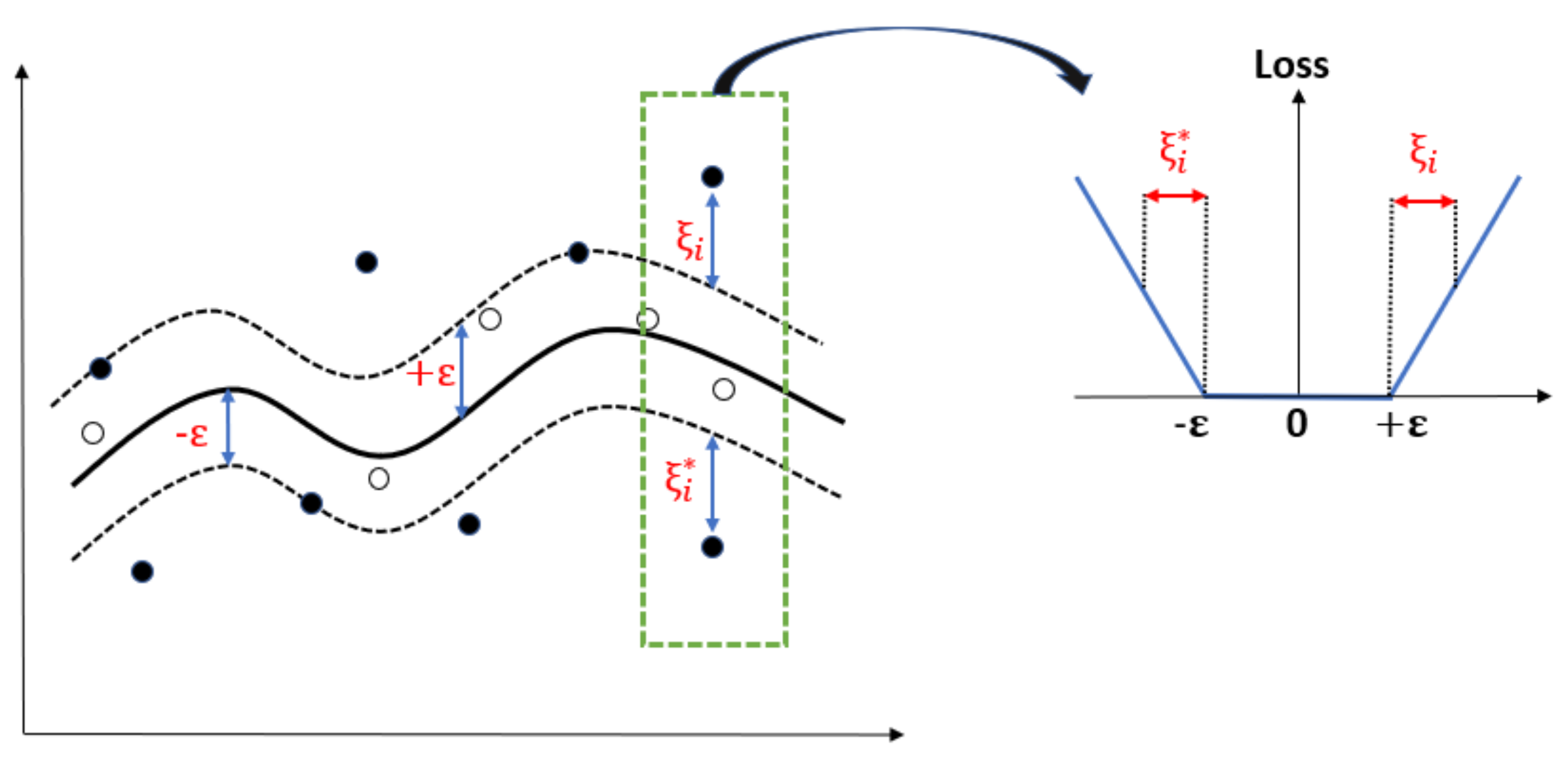This is called the ε-insensitive loss function, which is described by Equation (3)

$${\left|\mathsf{\xi }\right|}_{\epsilon }=\left\{\begin{array}{cc}0& if\left|\xi \right|<\epsilon \\ \left|\xi \right|-\epsilon & otherwise\end{array}\right.$$

(3)

The ε-insensitive loss function implies that only those training instances that are greater than ε in magnitude are used to support or determine the function f(x). Adding more training instances within the allowed deviation ε does not have any effect on the predictions. Figure 1 depicts the ε-insensitive loss function graphically.

Adding the objective of minimizing these deviations with Equation (2) results in the following formulation (Equation (4)):

$$\begin{gathered} Minimize\frac{{||w||}^2}{2}+C{\displaystyle \sum }_{i=1}^N({\mathsf{\xi }}_i+{\mathsf{\xi }}_i^{*}) \\ \mathrm{subject}\mathrm{to}\left\{\begin{array}{c}{y}_i-<w,\varphi \left(x_i\right)>-b\le \epsilon +{\mathsf{\xi }}_i\\ <w,\varphi \left(x_i\right)>+b-y_i\le \epsilon +{\mathsf{\xi }}_i^{*}\\ {\mathsf{\xi }}_i,{\mathsf{\xi }}_i^{*}\ge 0\end{array}\right. \end{gathered}$$

(4)

The value of the parameter ε controls the band’s width and can affect the number of support vectors used to construct the regression function. The parameter C is a constant that determines the trade-off between the two conflicting objectives of trying to make the slack variables as small as possible to reduce margin violation and the flatness of function f(x). Both ε and C are hyperparameters that must be tuned according to the dataset used to train the SVR model to achieve maximum efficiency on the test dataset. A common approach to select the optimal values for these hyperparameters is to use grid search where both ε and C are systematically varied and the cross-validation error monitored.

The convex quadratic optimization problem with linear constraints in Equation (4) is solved in its dual form where the constraints are handled by introducing Lagrange multipliers and taking partial derivatives of the Lagrangian with respect to ${\mathsf{\xi }}_i,{\mathsf{\xi }}_i^{*},w$ and $b$ and, thus, results in the support vector expansion form in Equation (6) by substituting Equation (5) into Equation (1).

$$w={\displaystyle \sum }_{i=1}^{\mathrm{N}}\left({\alpha }_i-{\alpha }_i^{*}\right)\varphi \left(x\right)$$

(5)

$$f\left(x\right)={\displaystyle \sum }_{i=1}^{\mathrm{n}}\left({\alpha }_i-{\alpha }_i^{*}\right)K\left(x_i,x\right)+b$$

(6)

where ${\alpha }_i$, ${\alpha }_i^{*}$ are Lagrangian multipliers and $K\left(x_i,x\right)$ is the kernel function. The kernel function enables the dot product to be performed in high dimensional feature space using low dimensional input data without knowing the transformation $\varphi$, which gives SVR the ability to model nonlinear datasets. The detailed mathematical procedure of the optimization procedure can be found in [12].

The Kernel function used in this paper is the Radial Basis Function (RBF) kernel. The hyperparameter gamma $\gamma$ in the function acts as a regularization that controls the spread of the function and must also be tuned during the training process. Given two instances of the input variables $x_i,x_j$, the RBF kernel evaluates nonlinearity between them, as described by Equation (7):

$$K\left(x_i,x_j\right)=e^{-\gamma {||x_i-x_j||}^2}$$

(7)

2.2. Hygrothermal Simulations

DELPHIN v5.9.5 was used to perform one-dimensional hygrothermal simulations in order to produce the data used for the SVR model’s development. DELPHIN 5 (coupled heat, air, moisture and pollutant simulation in building envelope systems) has the ability to solve one and two-dimensional problems and has been successfully validated with HAMSTAD Benchmarks 1 through 5 [13] and with experimental data [14]. The model uses either the full sorption isotherm or water retention function. Material properties are defined as a function of the volumetric moisture content and temperature. Climate data are entered as individual files for each climate variable. An important feature of DELPHIN is its ability to handle wind-driven rain deposition and solar radiation as part of its boundary conditions, as well as air leakage and moisture and heat sources.

Two types of buildings (a 3.5 story (10 m) wood frame residential building and a 13 story (~41 m) tall wood building) and three cities with contrasted climates located in Canada (Ottawa, Calgary, and Vancouver) were considered. Wall configurations, climate data, and simulation details are provided in the following sections.

2.2.1. Wall Assemblies

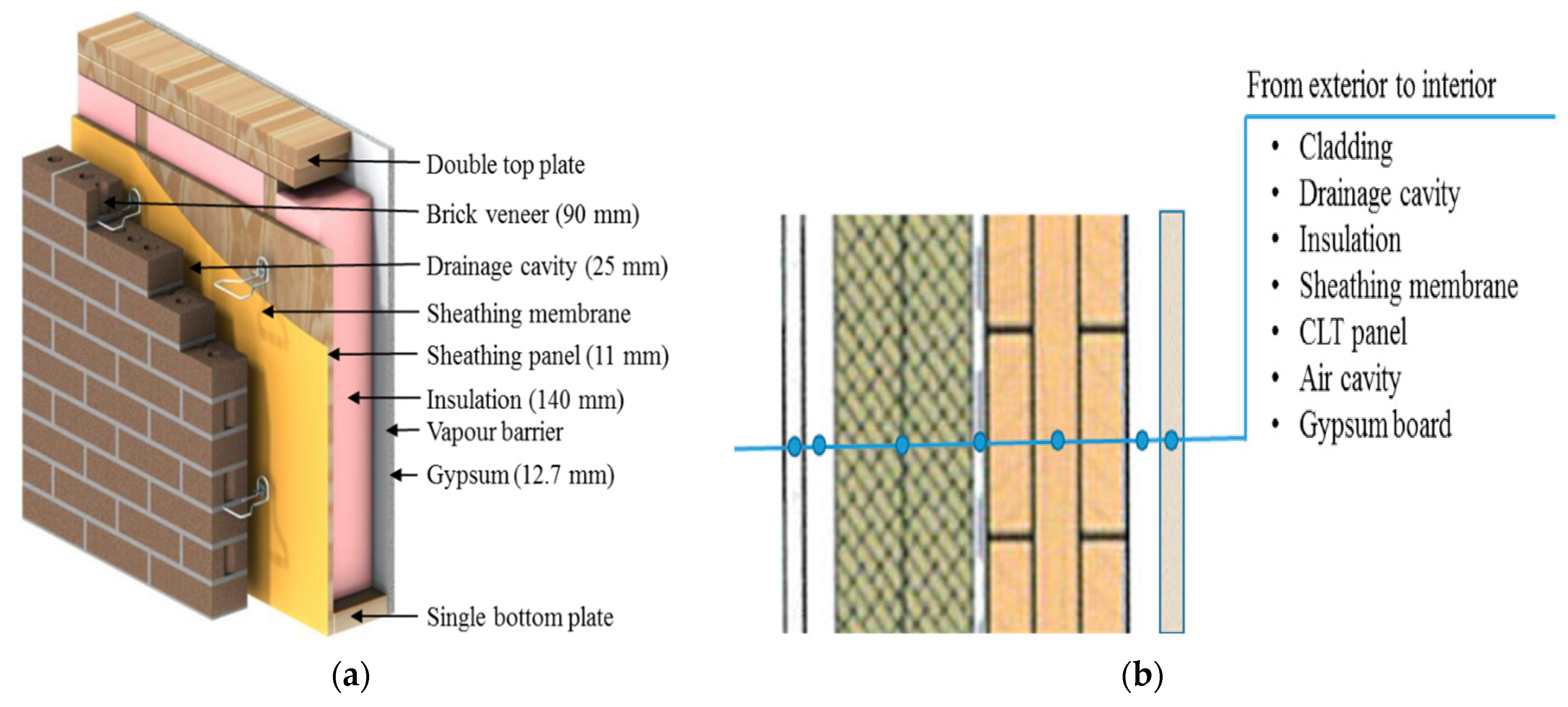
The wall assembly of the tall wood building consisted of (from exterior to interior): 11 mm fiberboard used as the cladding; 19 mm drainage cavity; two layers of mineral fiber insulation (2 × 64 mm in Ottawa and Vancouver and 2 × 89 mm in Calgary); a 0.15 mm sheathing membrane (spun bonded polyolefin); a 3-layer cross-laminated timber (CLT) made of spruce (95 mm); a 19 mm air cavity; and a 12.7 mm interior grade gypsum panel with latex primer and one coat of latex paint. That of the wood frame building was composed of (from exterior to interior): 90 mm brick cladding; a 25 mm drainage cavity; a 0.22 mm sheathing membrane (30 min asphalt impregnated building paper); an 11 mm Oriented Strand Board (OSB); 140 mm glass fiber insulation in stud cavity; a 0.15 mm polyethylene vapor barrier; and a 12.7 mm interior grade gypsum panel with latex primer and one coat of latex paint. Figure 2 shows the schematic of the wood frame and massive timber walls.

Material properties of wall components were obtained from [15] and [16]. CLT panel is composed of wood (spruce) layers glued together with an adhesive. The adhesive layer (assumed to extend 2 mm deep in the plank) was modeled with the same material properties as spruce, with the exception that the water vapor permeability and liquid water diffusivity were decreased by 50%. This was in line with the results obtained in [16] which showed that CLT’s vapor permeability and moisture diffusivity are substantially reduced in comparison with those of solid wood.

2.2.2. Climate Data

The ensemble climate data consisted of a modeled hourly time series of the climate variables necessary to undertake hygrothermal simulations for a baseline period spanning from 1986 to 2016 and 31-year-long future periods when global warming levels of 2 °C and 3.5 °C (with reference to the baseline period) are expected to be reached in the future. The climate datasets were generated to capture the effects of the internal variability of the climate on future climate projections in fifteen hourly realizations that were part of the datasets derived from the large ensemble of climates simulated by the Canadian Regional Climate Model (CanRCM4) version 4, each initialized under a different set of initial conditions in the second generation of the Canadian Earth System Model (CanESM2). A detailed description of the procedure used to generate the modeled historical and projected future climate can be found in [3].

For the purposes of this study, only some realizations from the historical (H: 1986–2016) and future (F: 2062–2092 corresponding to a scenario of global warming of 3.5 °C) periods were selected in each city for hygrothermal simulations. The hygrothermal simulations were performed over the 31 consecutive years of each selected realization to provide data for SVR modeling.

2.2.3. Simulation Setup

The simulations were performed on a one-dimensional configuration, far from and not including the spruce studs for the wood frame walls. The wall orientation in each city was selected as the direction in which the rainfall deposition from wind-driven rain was the highest for all the 31 years of each realization. The amount of rainwater impinging on the building façades was determined based on ASHRAE Standard 160 [17], assuming an exposure factor of 1.5 and 1.0, and a deposition factor of 1.0 and 0.5, for tall wood and wood frame buildings, respectively. Based on [17], 1% of wind-driven rain (WDR) was applied as a moisture source on the exterior surface of the sheathing membrane.

The initial conditions for relative humidity (RH) and temperature (T) were set to 80% and 21 °C, respectively, for all components. Indoor ambient T and RH were set as constant to 21 °C and 50%, respectively. Referring to the ISO 6946 Standard [18], the indoor convective heat transfer coefficient was set to 2.5 W/m²K, and the outdoor convective heat transfer coefficient was calculated using Equation (8):

α_ce = 4 + 4V

(8)

where α_ce is the outdoor convective heat transfer coefficient in W/m²K and V is the wind speed, corrected for the height of the building (m/s). The outdoor and indoor convective vapor transfer coefficients were calculated using the convective heat transfer and the Lewis number [19]. The indoor radiative heat transfer coefficient was set to 5.5 W/m²K [18], whereas the longwave exchange between the cladding surface and the environment was explicitly calculated, assuming a longwave emissivity of 0.9 for the surface and the surrounding ground and 1.0 for the sky. The ground surface temperature and albedo were set to the air temperature and 0.2, respectively. The shortwave absorption coefficient of the cladding was set at 0.6, assuming a red-colored surface. The air was assumed to be still in the air cavity between the drywall and the CLT, but air transfer in the drainage cavity of both walls was expected, having an air change per hour (ACH) of 10 in all cities.

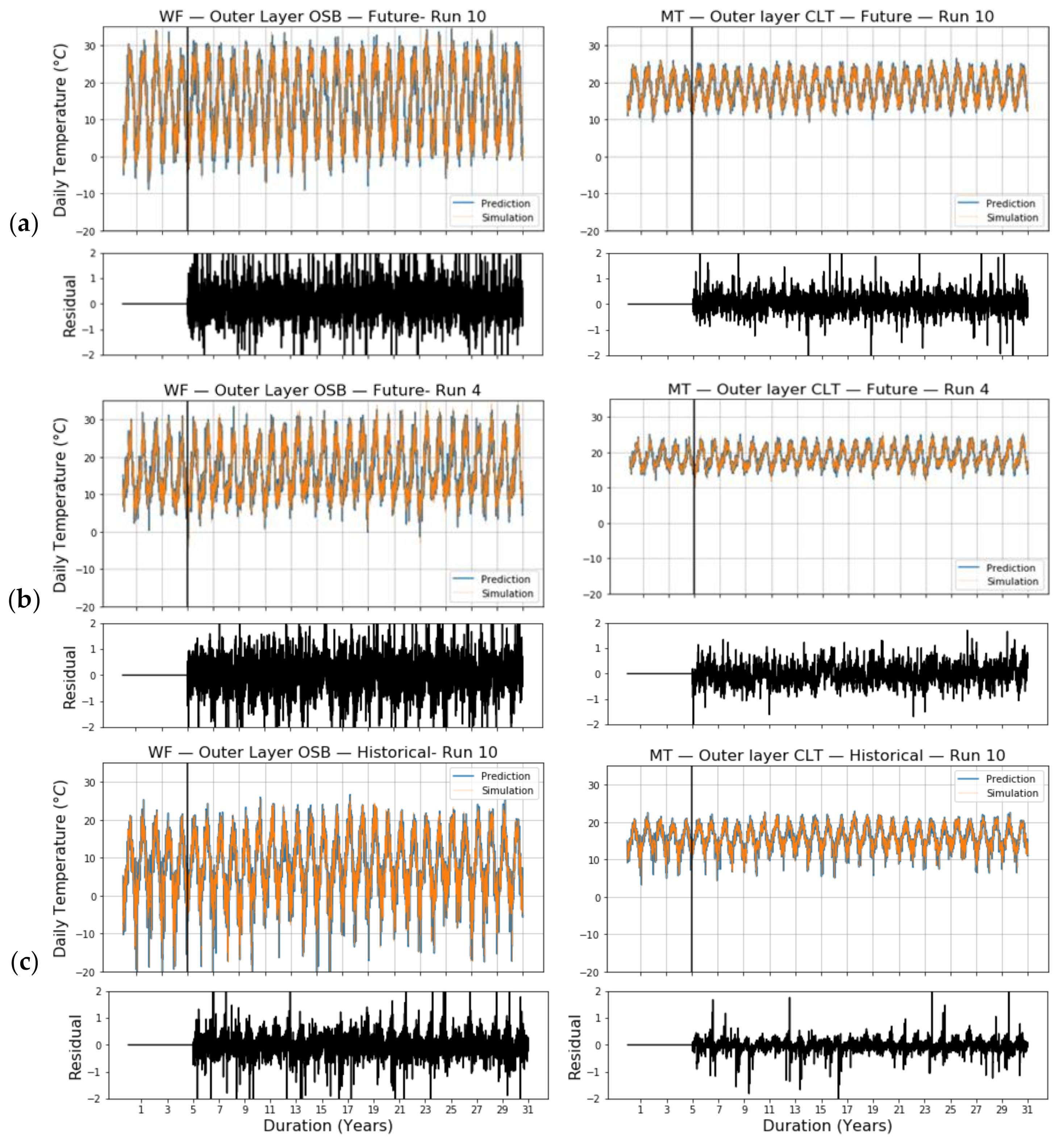
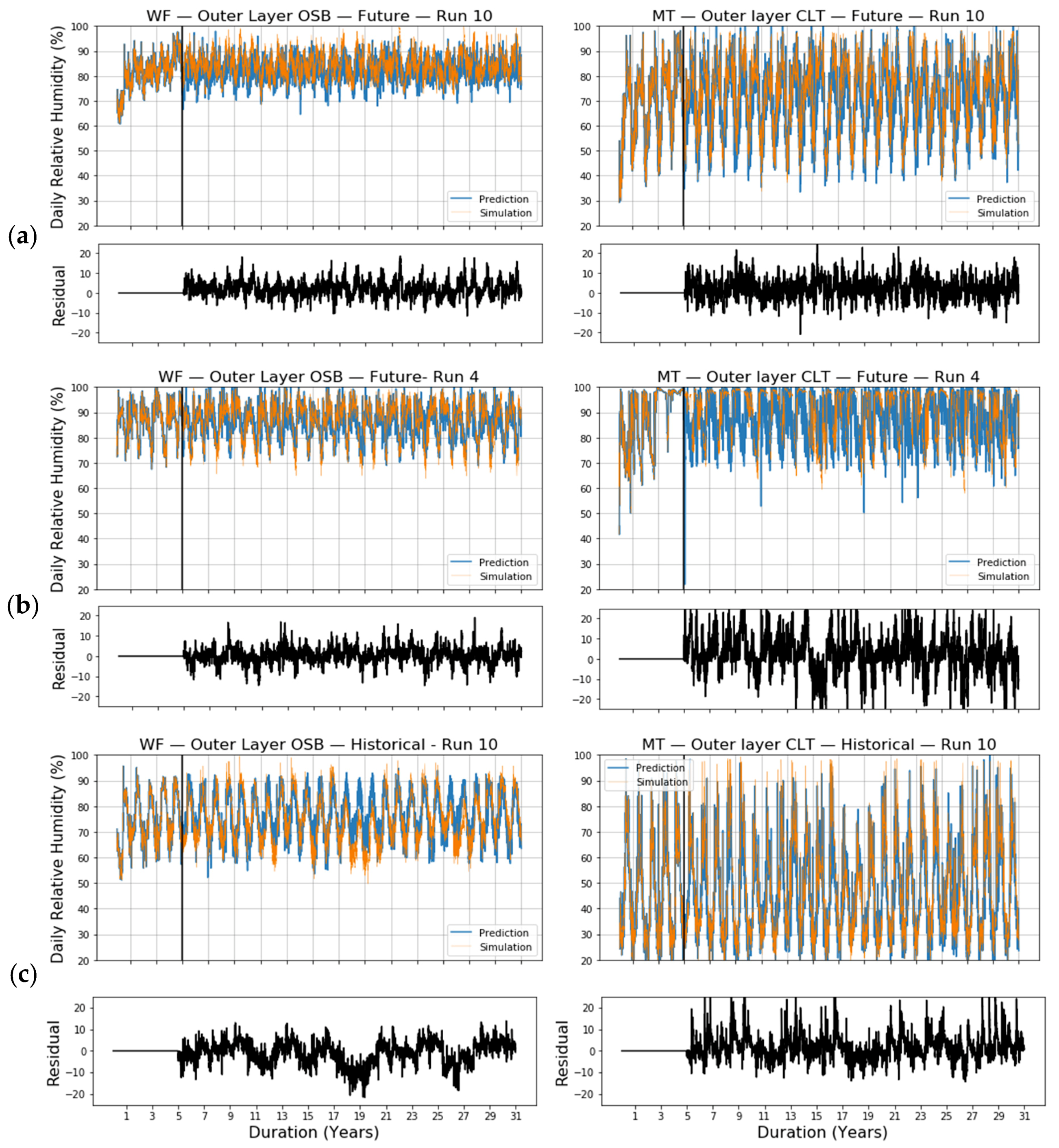
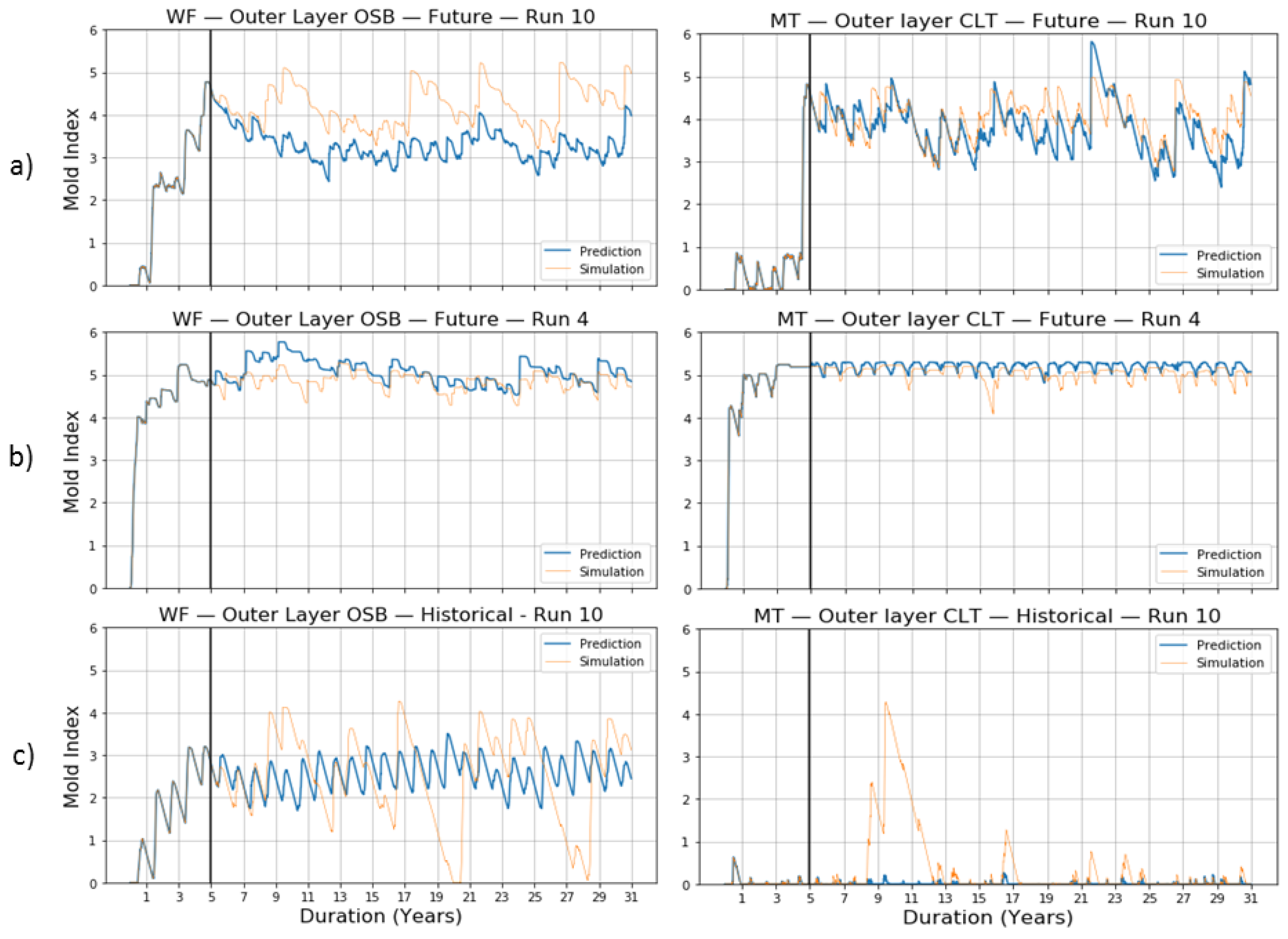
2.2.4. Critical Location for Moisture Performance Assessment

The outer layer (0.5 mm) of the CLT and OSB for tall wood and wood frame walls, respectively, were used as the critical location from which to extract hygrothermal simulations results, i.e., RH and T. These two variables were then used for calculating the mold growth index (MoI) with empirical formula found in [17]. The material RH and T obtained from hygrothermal simulations and the corresponding performance indicator (MoI) were used to benchmark the predicted responses and performance from the SVR model.

2.3. SVR Implementation

The following subsections explain the selection of the training set, the sliding window process, the hyperparameters and input variable selection, and the SVR model used to predict the hygrothermal responses. Three statistics are used to evaluate the performance: the coefficient of determination (R²), the mean square error (MSE), and the root mean square error prediction (RMSEP), which are calculated using Equations (9) to (11):

$$R^2=1-\frac{{{\displaystyle \sum }}_{i=1}^n{\left(y_i-y_i^{*}\right)}^2}{{{\displaystyle \sum }}_{i=1}^n{\left(y_i-\overline{y}\right)}^2}$$

(9)

$$MSE=\frac{1}{n}{\displaystyle \sum }_{i=1}^n{\left(y_i-y_i^{*}\right)}^2$$

(10)

$$RMSEP=\sqrt{\frac{1}{n}{\displaystyle \sum }_{i=1}^n{\left(y_i-y_i^{*}\right)}^2}$$

(11)

where $y_i$ is the true output from hygrothermal simulation, $y_i^{*}$ is the predicted output using SVR, $\overline{y}$ is the mean of the true output from hygrothermal simulation, and $n$ is the number of samples in the test set.

2.3.1. Selection of Training Set

From each 31-year time series dataset, the first 5 years were selected to be part of the training set and the remaining 26 years were used for validation. The main idea behind performing the study was to find an alternative to traditional simulation tools which can reduce simulation times. Choosing 15 years or higher to train the model defeats the purpose of doing this study, as many years will still need to be simulated in DELPHIN. Choosing fewer than 5 years will present a higher probability of not capturing the entire variation in the time series during the training phase. Therefore, selecting 5 to 10 years provides a good balance between speed and accuracy.

2.3.2. Sliding Window

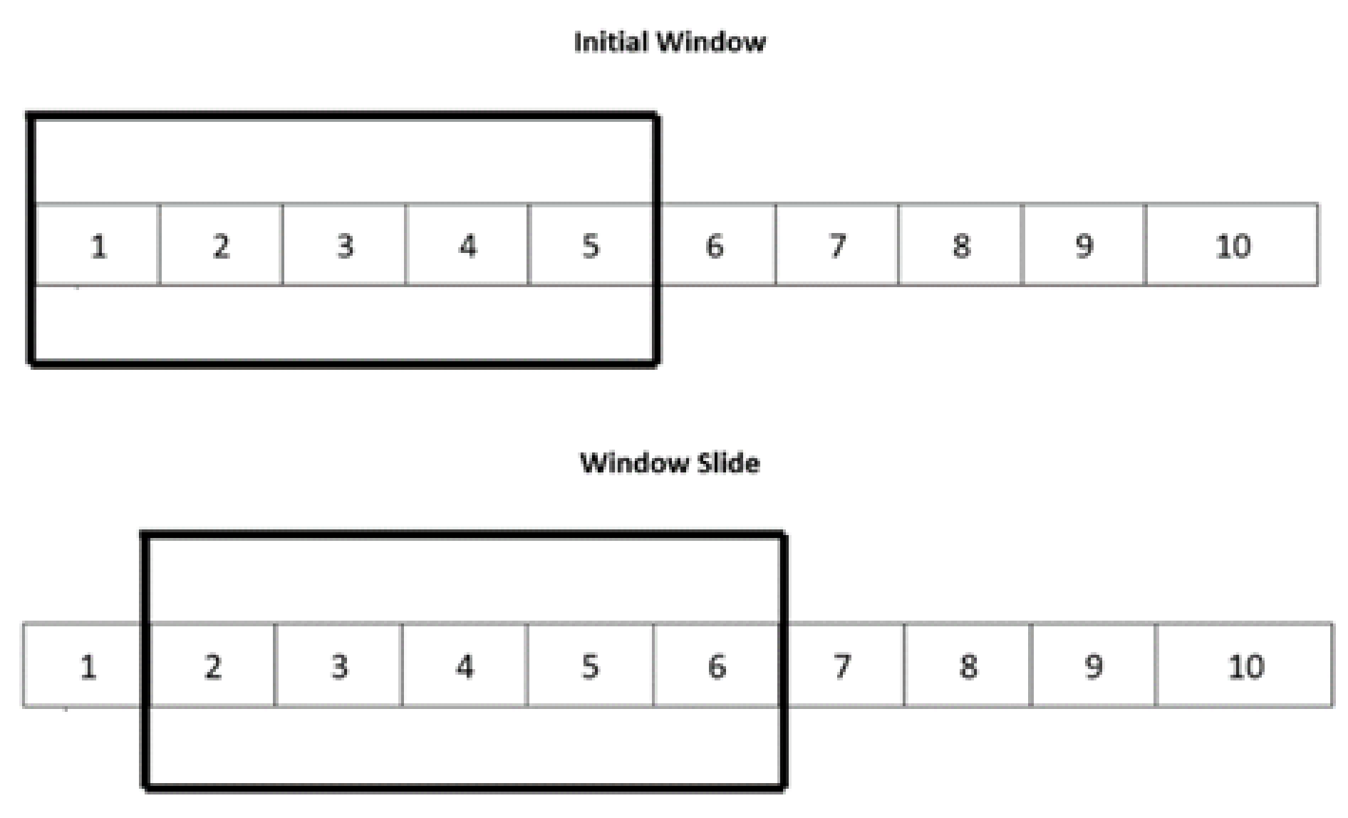
To handle the temporal dependencies that span multiple time steps, a sliding time window is used to reframe the time series problem as a supervised learning problem. A sliding window extracts all possible subsequences (of the same length) of a time series, generating a set of sliding windows of data. After selecting the first subsequence, the next subsequence is selected by moving the sliding window across the time dimension. This process is shown in Figure 3 with a window size or lag of 5. The number (1, 2, 3, …, 10) represents the observations of a time series. The initial sliding window captures the first 5 observations of the time series, which is the first subsequence. Then the window shifts right by 1 observation to cover the next subsequence of data. This process is repeated until all the possible subsequences can be generated from the time series.

The sliding window approach allows SVR to incorporate the temporal dependencies that span multiple timesteps between the outdoor climate variables and a hygrothermal response. The window size determines the number of previous time steps used as input to the model at the current time step. It is crucial to decide on the window’s optimum size, as observation outside the subsequences cannot predict the current time step. Therefore, a small number of trials were conducted with different lags to determine the optimal window size for the input climate variables. Some cities were randomly selected where SVR was trained and optimized (see Section 3.2) for the first 5 years, and forecasting performance was monitored for the next 26 years. The model’s accuracy is evaluated by R², which is calculated using Equation (9). 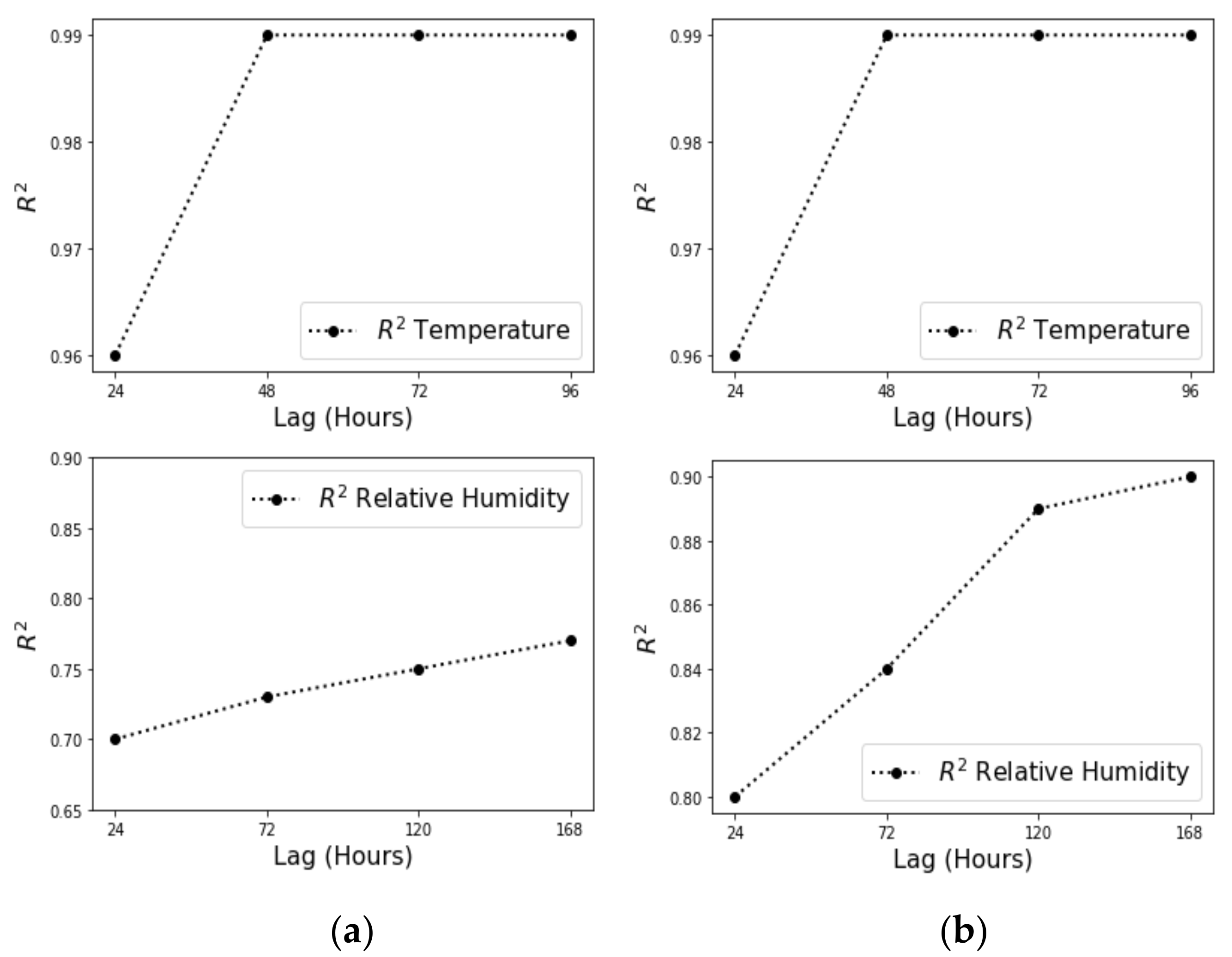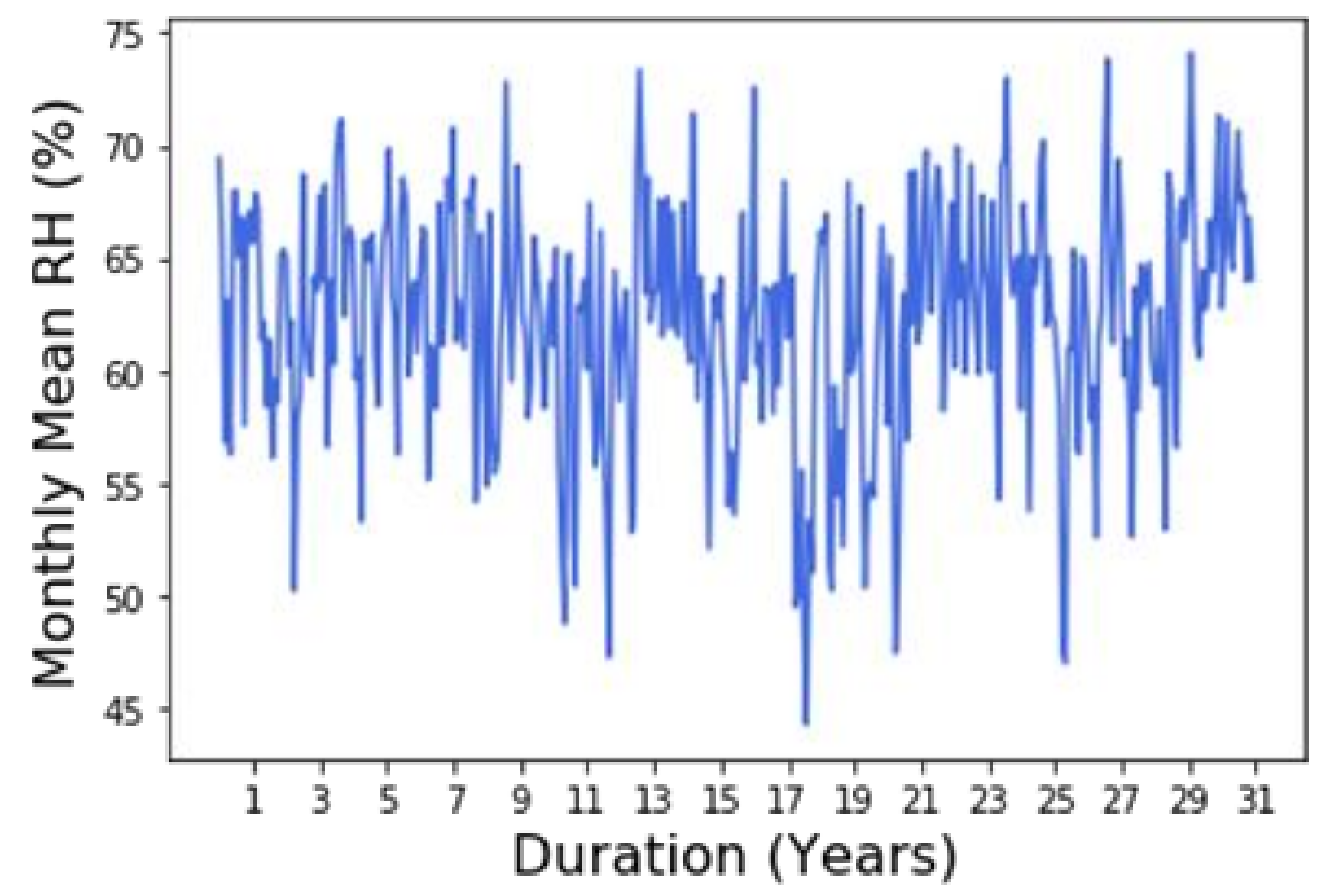Figure 4 shows the forecasting accuracy on the 26-test year using different lags for the two hygrothermal response variables in Ottawa (run 10 Historical Timeline).

The results suggest that temperature on the outer layer of OSB and CLT responds immediately to changes in the outdoor climatic conditions, with the past 48 h (2 days) being optimal. On the other hand, there is a significant delay between the outdoor conditions and response in RH on the outer surface of the OSB and CLT. The long delay for RH can be attributed to the relatively low moisture diffusivity of moisture in a porous medium compared to the high thermal diffusivity [20]. Capturing this long delay using the sliding window approach makes the input space huge, requiring extensive memory for storage and manipulation. For example, relative humidity predictions result in a transformed input space of (168 window size × 4 climate variables) 672 variables for each hour in the 31 year time series. Therefore, to ease the data processing, the window size for relative humidity was restricted to 168 h.

2.3.3. Hyperparameter Selection

The explanatory variables were standardized to have zero mean and unit variance. This preprocessing ensures all the variables are on the same scale, allowing for equal weight in the model.

To optimize the hyperparameters ε, $C$, and $\gamma$, a grid search was performed. The values of the parameters were systematically varied, and the 5-fold cross-validation error was evaluated for all the possible combinations of hyperparameter values. The parameter combinations, which yielded the lowest Mean Squared Error (MSE, Equation (10)), were then used for forecasting on the test set.

A summary of the selected parameter combination for the best SVR model is shown in

Table 1. Summary of results from SVR parameter estimation with RBF kernel.

Gamma	Cost	Epsilon	MSEP
0.0001	0.1	0.1	3.22
0.0001	10	0.1	3.05
0.0001	100	0.1	3.10
0.1	0.1	0.1	3.50
0.1	10	0.1	3.37
0.1	100	0.1	3.37
0.0001	0.1	0.5	3.27
0.0001	10	0.5	3.04
0.0001	100	0.5	3.17
0.1	0.1	0.5	3.48
0.1	10	0.5	3.43
0.1	100	0.5	3.43

. This example corresponds to the future timeline in Calgary city, run 10. The response is the temperature at the outer layer of the CLT. For this case, the lowest Mean Squared Error of Prediction (MSEP) was achieved using the RBF kernel with a gamma of 0.0001, a cost of 10, and an epsilon of 0.5. Therefore, this parameter combination was used in the forecasting phase.

2.3.4. Input Variable Selection

Least Absolute Shrinkage and Selection Operator (LASSO) is a popular technique used for variable selection and has been effective in the context of auto-regressive time series modeling [21,22]. LASSO belongs to a class of shrinkage methods that fit a model containing all the predicators but constraints or regularizes the coefficient estimates. In the case of LASSO, it is the L1 regularization that shrinks some of the coefficient estimates to be exactly equal to zero, thereby performing feature selection. To understand the complete procedure, the reader can refer to [23].

LASSO was performed using the glmnet package [24] in R [25] to select a subset of the most contributing climate variables among the 8 climate variables considered, i.e., temperature (°C), relative humidity (%), wind speed (m/s), wind direction (°), direct radiation (W/m²), diffuse radiation (W/m²), wind-driven rain (kg/m²s) and cloudiness index. The 31-year hourly time series data for the climate variable was restructured using the sliding window according to the optimal lag found for each hygrothermal response. The LASSO parameter, lambda, was then chosen using 5-fold cross-validations over a grid of possible lambda values. The lambda value that resulted in the smallest cross-validated error was picked, and the associated regression coefficient was then used to select the most contribution variables. 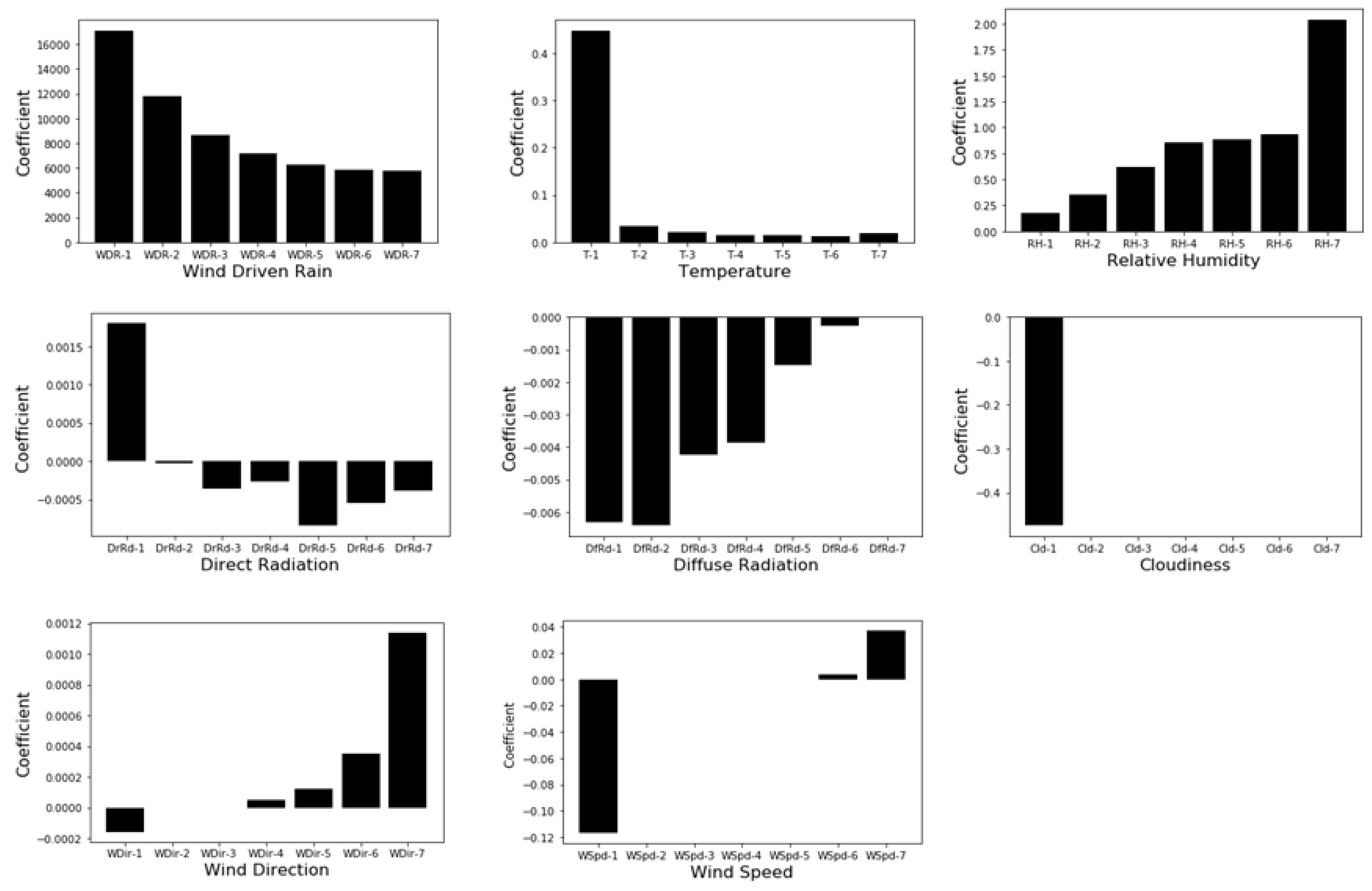Figure 5 shows the standardized regression beta coefficient associated with the lagged climate variable. This example corresponds to the historical timeline in Ottawa city, run 10. The response is the relative humidity at the outer layer of the OSB for the brick-clad wood frame wall. Notice that to ease the interpretation of the results, each time step represents the daily contribution of the climate variable obtained by summing the hourly coefficients. As seen in Figure 5, the most contributing variables are WDR, RH, and T. Variables, such as diffuse and direct radiations, cloudiness, wind speed, and wind direction, show little to no contribution in explaining the variation in the response. Other cases studied showed a high contribution of the direct radiation, especially for the cases where default orientation was toward the north. Similar results were observed when analyzing the temperature of the exterior surface of OSB. Therefore, WDR, RH, T, and direct radiation were selected and used in this study.

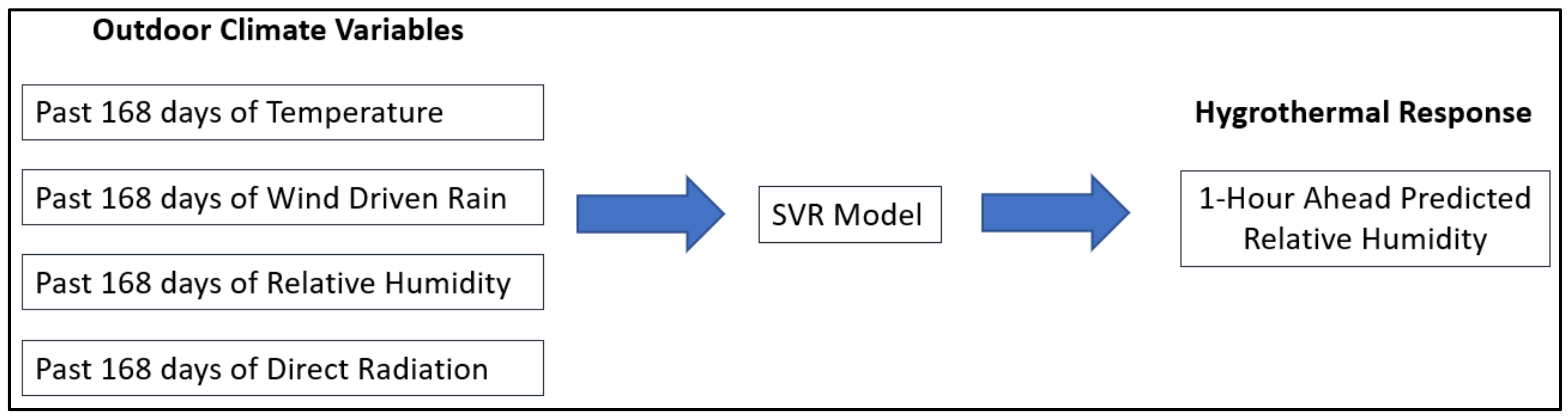
2.3.5. Construction of SVR Model

The SVR model was constructed using the four selected outdoor climate variables, i.e., T, RH, WDR, and direct radiation, which were reorganized according to the optimal lag using the sliding window to model each of the hygrothermal responses. The procedure used to predict RH is shown in Figure 6. A similar procedure was used to predict T, but with a lag of 48 h for the outdoor climate variables. SVR was performed using the library ThunderSVM [26] in R [25].

The SVR-predicted hourly T and RH values at the outer layer of OSB or CLT were used to calculate the mold index and compare alongside the mold index derived from the simulated T and RH values from DELPHIN. The hourly frequency was used for both T and RH since the mold growth index calculation model requires hourly values.

3. Results and Discussion

Figure 7 and Figure 8 compare simulation results from DELPHIN and SVR predictions for a 31-year long time series of temperature and relative humidity, Figure 9 shows the outdoor relative humidity profile in Calgary, and Figure 10 compares the subsequent mold index predictions for the wood frame (WF) and massive timber (MT) walls in the three cities considered. The results are those obtained using future climate data in Ottawa (run 10) and Vancouver (run 4) and historical climate data in Calgary (run 10). They were selected to represent the best and worse scenarios observed. The black vertical line indicates the end of the training phase, the first 5 consecutive years. The residual plots show the deviation in the prediction for temperature and relative humidity. The prediction statistics are shown in

Table 2. Summary statistics for forecasting temperature for the three cities.

City	Wood Frame Wall		Massive Timber Wall
	RMSEP	R2	RMSEP	R2
Ottawa	0.12	0.99	0.05	0.99
Calgary	0.07	0.99	0.04	0.99
Vancouver	0.11	0.99	0.06	0.99

and

Table 3. Summary statistics for forecasting relative humidity for the three cities.

City	Wood Frame Wall		Massive Timber Wall
	RMSEP	R2	RMSEP	R2
Ottawa	0.82	0.46	1.03	0.86
Calgary	1.23	0.58	1.13	0.89
Vancouver	0.72	0.75	1.75	0.27

for temperature and relative humidity, respectively.

3.1. Temperature Profile

The results obtained for temperature are shown in Figure 7. Temperature profiles at the outer layer of OSB or CLT are generally well predicted in all the three cities considered (R² of 0.99). This good overlap can be attributed to the stationary nature of the outdoor and material temperature time series. Comparing the results of the two walls reveals a wider range of temperature variation in OSB than CLT. In fact, the OSB panel is subjected to direct effects of outdoor conditions due to ventilation in the drainage cavity, while the CLT is preserved from the direct influence of outdoor conditions due to outboard insulation. This leads to slightly better predictions for CLT in mass timber wall (residuals between ±1 °C and RMSEP of 0.04 to 0.06 °C) than for OSB in wood frame wall where peaks and valleys are slightly over- or under-predicted (residuals between ±2 °C and RMSEP of 0.07 to 0.12 °C), in all three cities.

3.2. Relative Humidity Profile

Figure 8 shows the results obtained for relative humidity. SVR predictions vary from city to city but are generally better for the outer layer of OSB in wood frame walls (residuals between ±10%) than for the outer layer of CLT in massive timber walls (residuals up to ±20%). This is contrary to the results obtained for temperature, where SVR predictions are better for the outer layer of CLT in mass timber walls than for the outer layer of OSB in the wood frame walls. These contradictory results for RH can be explained by (1) the lower moisture diffusivity compared to heat diffusivity, and (2) the higher distance from the drainage cavity to the outer layer of CLT in massive timber walls compared to the outer layer of OSB in the wood frames. On another side, the time lag for relative humidity was not optimal and limited to 168 hours, as explained in Section 3.1.

For the outer layer of CLT panel in mass timber walls, the SVR predictions are better in Ottawa (RMSEP of 1.03%, and R² of 0.86) followed by Calgary (RMSEP of 1.13% and R² of 0.89) followed by Vancouver, where the SVR predictions are particularly worse (RMSEP of 1.75% and R² of 0.27). For the outer layer of OSB in the wood frame wall, the SVR predictions are this time better in Vancouver (RMSEP of 0.72% and R² of 0.75) followed by Ottawa (RMSEP of 0.82 and R² of 0.46) and then Calgary (RMSEP of 1.23% and R² of 0.58).

The relatively worse SVR predictions for relative humidity in Calgary can be attributed to extreme climatic conditions that occur outside the SVR training phase. As seen in Figure 9, between years 8 to 13, 17 to 21, and 25 to 26, there are unique outdoor relative humidity conditions that occur after the first five years. SVR’s model could not capture these extreme, lowest humidity conditions during the training. While the discrepancies observed in Calgary can be explained by the sudden change in RH after the first 5 years, it is difficult to explain the worse performance of SVR for the outer layer of CLT in Vancouver, as the climate data did not show any unusual patterns.

3.3. Mold Index Profile

Figure 10 shows the mold growth index values calculated using the material temperature and RH obtained from DELPHIN simulations and SVR predictions. Despite the poor prediction of relative humidity by SVR, the results for the mold growth index are acceptable for the case of the massive timber wall in Ottawa and both walls in Vancouver. The mold growth index values are underestimated for the case of the wood frame wall in Ottawa. In Calgary, there are large discrepancies between the DELPHIN and SVR model results during the years where there was an abrupt change in the outdoor RH.

There are two input variables for mold calculation: temperature and relative humidity (RH). Temperature is generally well predicted, with residuals varying from −2 to 2 °C. In some cases, such as in Ottawa and Vancouver, RH is relatively poorly predicted but the mold output prediction is acceptable. This could be due to the artefacts of the mold model which starts calculating the mold index when RH values are greater than the threshold of 80%. For example, if the actual RH is 60% while the predicted value is either 50% or 70%, there is no impact on the mold index calculation. Moreover, when there are favorable mold growth conditions, for example, when the actual RH is 90%, and the predicted value is either 85% or 95%, it may happen that this error of 5% may not impact the resulting mold index significantly.

3.4. Time Comparison of DELPHIN Simulations and SVR Predictions

SVR requires time for data preparation, training, and prediction. When the script is ready data preparation can take up to 20 min, training up to 30 min, and prediction up to 20 min, all depending on the lag used. This cumulates to more than one hour for a series of 31 years, with 5 initial years used for training and prediction for the next 26 years. This time is comparable to the time needed to prepare and run 31 consecutive years in DELPHIN for a one-dimensional setting. However, a 2D simulation in DELPHIN for 31 consecutive years would require several hours, and it would be beneficial to use SVR if the results were consistent for all the cases.

4. Conclusions

This paper explored the potential of a machine learning algorithm, the Support Vector Regression (SVR), to forecast long-term hygrothermal responses (e.g., temperature, relative humidity) of the building envelope. DELPHIN was used to perform hygrothermal simulations using 31-year long series of climate data in several cities across Canada for a wood frame and massive timber wall. Then, the first 5 years of the series were used in each case to train the model, which was then used to forecast the hygrothermal response for the remaining years of the series. Trials were conducted with different lags of climate variables to determine the optimal sliding time window, which allowed SVR to capture time implicitly. The selection of essential climate variables was performed using LASSO. The optimal hyperparameter associated with SVR was obtained using cross-validation and grid search. Finally, the results obtained were validated with the actual simulation results from DELPHIN.

The results for both temperature and relative humidity showed that SVR is effective in forecasting the hygrothermal responses on a long climate data series under certain conditions. The temperature was well predicted for all the cases, irrespective of the type of wall or city. This is attributed to the stationary nature and short lag time, i.e., temperature reacts quickly to changes in outdoor climate conditions. By contrast, relative humidity shows long-term dependencies on the outdoor climate and is poorly predicted. For cities such as Ottawa and Vancouver where there is no drastic change in the climate throughout the 31-year series, mold index predictions are acceptable; meanwhile, in Calgary, where there is a significant dry period that occurs after the training phase, there is a large discrepancy between the SVR and DELPHIN results.

Some limitations associated with the approach presented in this study are observed. Firstly, applying the sliding window to the input variables makes the input space huge. Secondly, training the SVR model still requires minimally 3 to 5 years of the hygrothermal response to be obtained using a traditional simulation tool. Moreover, the full range of variability of the climate variables should be present in these first 3 to 5 years; otherwise, the prediction can be inconsistent. Consequently, the strategy presented in this paper shows limitations that prevent it from replacing the time-consuming traditional simulation tools. However, this study’s findings can be used to select a more suitable machine learning approach, perhaps recurrent neural networks that can address the shortcomings of SVR and the sliding window.

References

1. Intergovernmental Panel on Climate Change (IPCC). AR5 Synthesis Report: Climate Change 2014; IPCC: Geneva, Switzerland, 2014. [Google Scholar]
2. Bizikova, L.; Neale, T.; Burton, I. Canadian Communities’ Guidebook for Adaptation to Climate Change; Environment Canada: Ottawa, ON, Canada, 2009.
3. Gaur, A.; Lacasse, M.; Armstrong, M. Climate data to undertake hygrothermal and whole building simulations under projected climate change influences for 11 canadian cities. Data 2019, 4, 72. [Google Scholar] [CrossRef] [Green Version]
4. Hagentoft, C.E.; Harderup, E. Climatic influences on the building envelope using the π factor. In IEA-Annex 24 Hamtie Task 2, Environmental Conditions. Closing Seminar; International Energy Agency (IEA): Helsinki, Finland, September 1996. [Google Scholar]
5. Zhou, X.; Derome, D.; Carmeliet, J. Robust moisture reference year methodology for hygrothermal simulations. Build. Environ. 2016, 110, 23–35. [Google Scholar] [CrossRef]
6. Cornick, S.; Djebbar, R.; Dalgliesh, W.A. Selecting moisture reference years using a Moisture Index approach. Build. Environ. 2003, 38, 1367–1379. [Google Scholar] [CrossRef]
7. Salonvaara, M.; Sedlbauer, K.; Holm, A.; Pazera, M. Effect of selected weather year for hygrothermal analyses. In Proceedings of Thermal Performance of The Exterior Envelopes of Whole Buildings XI Clearwater, FL, USA, 5–9 December 2010; American Society of Heating, Refrigerating and Air-Conditioning Engineers, Inc.: Atlanta, GA, USA, 2010. [Google Scholar]
8. Freire, R.; Santos, G.; Coelho, L. Hygrothermal dynamic and mould growth risk predictions for concrete tiles by using least squares support vector machine. Energies 2017, 10, 1093. [Google Scholar] [CrossRef] [Green Version]
9. Dong, B.; Li, Z.; Rahman, S.M.; Vega, R. A hybrid model approach for forecasting future residential electricity consumption. Energy Build. 2016, 117, 341–351. [Google Scholar] [CrossRef]
10. Cortes, C.; Vapnik, V. Support-vector networks. Mach. Learn. 1995, 20, 273–297. [Google Scholar] [CrossRef]
11. Schölkopf, B.; Smola, A.; Bach, F. Learning with Kernels: Support Vector Machines, Regularization, Optimization, and Beyond; MIT Press: Cambridge, MA, USA, 2008. [Google Scholar]
12. Smola, A.J.; Schölkopf, B. A tutorial on support vector regression. Stat. Comput. 2004, 14, 199–222. [Google Scholar] [CrossRef] [Green Version]
13. Sontag, L.; Nicolai, A.; Vogelsang, S. Validierung der solverimplementierung des hygrothermischen simulations programms. In DELPHIN; Institute of Building Climatology (TU Dresden): Dresden, Germany, 2013. [Google Scholar]
14. Langmans, J.; Nicolai, A.; Klein, R.; Roels, S. A quasi-steady state implementation of air convection in a transient heat and moisture building component model. Build. Environ. 2012, 58, 208–218. [Google Scholar] [CrossRef]
15. Kumaran, M.K.; Lackey, J.C.; Normandin, N.; Tariku, F.; van Reenen, D. A Thermal and Moisture Transport Property Database for Common Building and Insulating Materials: Final Report from ASHRAE Research Project 1018-RP; American Society of Heating, Refrigerating and Air-Conditioning Engineers, Inc.: Atlanta, GA, USA, 2002. [Google Scholar]
16. Al Sayegh, G. Hygrothermal Properties of Cross-Laminated Timber and Moisture Response of Wood at High Relative Humidity. Master’s Thesis, Carleton University, Ottawa, ON, Canada, 2012. [Google Scholar]
17. ASHRAE. ASHRAE Standard 160-2016. (n.d.). Criteria for Moisture-Control Design Analysis in Buildings; American Society of Heating, Refrigerating and Air-Conditioning Engineers, Inc.: Atlanta, GA, USA, 2016. [Google Scholar]
18. ISO 6946. Building Components and Building Elements-Thermal Resistance and Thermal Transmittance-Calculation Methods; International Organization for Standardization: Geneva, Switzerland, 2017. [Google Scholar]
19. Incropera, F.P.; DeWitt, D.P. Fundamentals of Heat Andmass Transfer, 4th ed; John Wiley and Sons: New York, NY, USA, 1996. [Google Scholar]
20. Hugo, H. Building Physics. Heat, Air and Moisture. Fundamentals and Engineering Methods with Examples and Exercises, 2nd ed.; Wilhelm Ernst & Sohn: Berlin, Germany, 2012. [Google Scholar]
21. Nardi, Y.; Rinaldo, A. Autoregressive process modeling via the lasso procedure. J. Multivariate Anal. 2011, 102, 528–549. [Google Scholar] [CrossRef] [Green Version]
22. Iturbide, E.; Cerda, J.; Graff, M. A comparison between LARS and LASSO for initialising the time-series forecasting auto-regressive equations. Procedia Technol. 2013, 7, 282–288. [Google Scholar] [CrossRef] [Green Version]
23. Tibshirani, R. Regression shrinkage and selection via the lasso. J. Royal Stat. Soc. Ser. B Methodol. 1996, 58, 267–288. [Google Scholar] [CrossRef]
24. Friedman, J.; Hastie, T.; Tibshirani, R. Regularization paths for generalized linear models via coordinate descent. J. Stat. Software 2010, 33, 1–22. [Google Scholar] [CrossRef] [Green Version]
25. R Core Team. R A Language and Environment for Statistical Computing; R Foundation for Statistical Computing: Vienna, Austria, 2019. [Google Scholar]
26. Wen, Z.; Shi, J.; Li, Q.; He, B.; Chen, J. ThunderSVM: A fast SVM library on GPUs and CPUs. J. Mach. Learn. Res. 2018, 19, 797–801. [Google Scholar]
Figure 1. Loss Setting for Nonlinear SVR. The right side of the image shows soft ε-insensitive setting as described in [11] for SVR. Any values between −ε and +ε are assigned a loss 0 and values outside the range is assigned a loss of ξ ε .
Buildings 11 00188 g001
Figure 2. Composition of the wall types considered in this study (a) wood frame wall (WF), (b) massive timber wall (CLT).
Buildings 11 00188 g002
Figure 3. Process of sliding window.
Buildings 11 00188 g003
Figure 4. Forecasting accuracy for temperature and relative humidity by using different lags for climate variables: (a) wood frame (WF) and (b) massive timber (MT) walls.
Buildings 11 00188 g004
Figure 5. Contribution of the climate variables for the past 7 days to explain the variation in relative humidity at the exterior surface of OSB.
Buildings 11 00188 g005
Figure 6. A summary of the procedure used to generate relative humidity at each timestep.
Buildings 11 00188 g006
Figure 7. Comparisons of SVR predictions and hygrothermal simulation results for the temperature of the outer layer of OSB in wood frame (WF) and the outer layer of CLT in mass timber (MT) walls in the cities of (a) Ottawa, (b) Vancouver, and (c) Calgary.
Buildings 11 00188 g007
Figure 8. Comparisons of SVR predictions and hygrothermal simulation results for the relative humidity of the outer layer of OSB in wood frame (WF) and outer layer of CLT in mass timber (MT) walls in the cities of (a) Ottawa, (b) Vancouver, and (c) Calgary.
Buildings 11 00188 g008
Figure 9. Outdoor relative humidity profile for run 10 in historical climate data of the city of Calgary.
Buildings 11 00188 g009
Figure 10. Comparisons of mold index calculated using temperature and relative humidity predicted from SVR and simulated using DELPHIN for the outer layer of OSB in wood frame (WF) and outer layer of CLT in mass timber (MT) walls in the city of (a) Ottawa, (b) Vancouver, and (c) Calgary.
Buildings 11 00188 g010