An Assessment Methodology for the Evaluation of the Impacts of the COVID-19 Pandemic on the Italian Housing Market Demand

Abstract

Due to the forced changes that the COVID-19 pandemic has had in many aspects of ordinary life (working, social life, training and learning in schools etc.), the characteristics of domestic spaces have significantly modified buying, selling and renting decisions in the real estate market. The aim of this research was to structure a methodology, articulated into four steps, to assess the variation that has occurred in residential market demand as a result of COVID-19 anti-contagion measures, with regard to six metropolitan Italian cities. We considered two samples of properties for each city, the first referencing the pre-COVID-19 pandemic spread and the second collected in the current situation. Consequently, we were able to determine variations in residential market appreciations through the application of a regressive econometric technique. The obtained results highlighted the relevance assumed by indoor acoustic and thermal comfort property factors, compared with the pre-COVID-19 condition. The proposed methodology could be useful to support the public and private entities involved in urban investment decision-making processes, allowing us to identify the most appreciated factors of the residential real estate market demand, in order to improve the conditions of existing and future assets and reduce the related risk levels.

1. Introduction

Starting in the first half of 2019, the COVID-19 pandemic has spread rapidly worldwide and, in order to minimize contagion, governments have applied many of measures that, most of all, have forced people to stay at home. This has changed the shape of ordinary lives, requiring people to continue some activities in the domestic space [1,2,3]. In this way, rooms such as the living room, the bedrooms and the kitchen have had to accommodate functions for which they may not have been equipped: in many cases they have been transformed into working spaces, gyms, and meeting rooms. The impossibility of conducting outdoor activities, on the other hand, has meant that balconies, terraces or condominium green outdoor spaces have become the only way out of the house, and they too have been transformed into gyms, places of leisure, relaxation or work, and meeting areas. In other words, domestic spaces that previously performed a certain number of functions, strictly related to the ordinary daily activities of people before the restrictive measures of COVID-19, had to welcome new ones, often proving to be inadequate. Moreover, spaces such as balconies or terraces, not always present in all types of residential buildings, have been found to be essential for many reasons—from those relating to mental and physical health to those associated with domestic activities—when the anti-contagion measures were very restrictive (i.e., in lockdown). The fear and uncertainty about the future developments of the pandemic, still ongoing, has led to a more global introspective vision. Before the beginning of the COVID-19 pandemic, most daily time took place outside of the home; therefore, the possibility of a further restrictive lockdown has changed the perception of which domestic spaces are viewed as desirable [4,5,6]. According to a recent Forbes analysis in America, “the hottest housing markets in the new landscape are cities which offer desirable amenities—larger homes, leafy neighborhoods, access to the outdoors, walkability and proximity to grocery stores—in a more affordable package, and home buyers still want to be within commuting distance of large employment centers, but with the prevalence of remote work, they are willing to extend the distance from urban downtowns” [7].

Italy is one of the countries that has imposed restrictive anti-contagion measures for the longest time, particularly in the most densely populated cities such as Milan, Turin, Rome and Naples, which were among those with the highest number of infections and deaths, together with Florence and Catania [4]. This condition clashed with the characteristics of the existing residential real estate, characterized by a high average age (60 years), medium–low energy efficiency, an average area of 67 m² per resident which, in terms of average area per house, becomes about 117 m². In this situation, there were also some socio-economic characteristics: 27% of the population were living in overcrowded houses, with an average number of members per family of 2.28, rising to 2.68 in some territorial centers, such as the province of Naples and Catania. This was in addition to an average poverty index of 21.4% in 2020 [8,9]. To avoid (or minimize) interpersonal contacts, most work activities—especially those not related to the agri-food, logistics and health sectors—all school and educational courses (public and private), all sport events (competitive and amateur), and most religious gatherings (with the exception of funerals) often needed to be reproduced in some way at home. Consequently, the digitization process of many of these activities has been forced to rapidly spread, and will grow further, involving about 8.2 million workers [10,11]. Remote work, e-learning, and the use of online services, takes the shape of new ordinary living, becoming the only way to be able to continue everyday activities. However, these general conditions have caused many problems, as the critical fragility of these house–space systems emerged, with the spaces being inadequate to perform their new functions [12,13,14,15]. Significant changes have occurred in the perception of domestic spaces and their prerequisites. New potential market demand has been defined, favoring (i) the possibility of articulating housing units in a multifunctional way; (ii) the availability to equip a space dedicated to remote working that is adequate from the point of view of privacy and ergonomic comfort; (iii) the presence of private outdoor spaces, to carry out leisure activities in external areas; (iv) the presence of condominium services such as gyms, multifunctional rooms, and box lockers, all factors that pertain to the intrinsic characteristics of the properties [16,17]. In the Italian context, different studies that have analyzed the preferences of domestic space users in October 2020 have identified the following preferences for some elements of residential properties: private garden (58%), parking space (51%), living–kitchen (48%), terrace (47%), living room (46%), children’s room (45%), two or more bathrooms (45%) [18]. The results obtained were validated by an analysis developed by the Bank of Italy in 2021 [19] that examined people’s preferences for some residential space characteristics. The new preferences are oriented towards spaces previously considered secondary, if not downright irrelevant (such as the private garden or the balcony), strongly conditioning the demand of the residential real estate market. Existing offers experienced a strong cut, conditioned by the market’s ability to respond to the new requirements expressed by buyers [20]. The houses that fulfilled the new market demand became the main target, while the others were outclassed. Furthermore, the fear of a new stringent lockdown, with the pandemic still in progress, has pushed buyers to invest more capital in homes that reflect their wishes. This condition has generated a decrease in the real estate prices of homes with features that before the COVID-19 situation had inaccessible or high selling prices, and an increase in price for the properties with new desirable features [20,21].

These emerging trends based on new intrinsic factors, including the specificities of houses rather than neighborhood spaces, must be analyzed through the application of efficient tools capable of identifying the most important factors, in terms of the impact and variation on the selling prices of houses, induced by COVID-19 on the local market. This could be useful to reduce the risk of creating large residential properties that are no longer necessary because they are inadequate to the demand preferences, a condition that would lead to an increase in urban decay, in contrast with the objectives of the 2030 Agenda [22].

The present research pertains to the context outlined, and is aimed to structure a methodology that consists of orderly and distinct phases for the assessment of the likely effects of anomalous events—like the COVID-19 pandemic—on the real estate market. Based on a genetic algorithm able to detect the most important factors affecting selling prices, two samples of residential properties were collected for each of the six Italian cities that (i) have been most affected by the pandemic, (ii) have the greatest overcrowding index and (iii) have the residential assets that reflect the average national intrinsic factors. Two phases for each city were considered: the first referenced the second half of 2019 (“pre-COVID-19 pandemic”), the second, instead, concerned the first half of 2021 (period in which the pandemic is still in progress “COVID-19 pandemic in progress”). The purpose of considering these two situations was to verify the existence of changes in the dynamics in the reference market and identify the factors that most influenced investment choices, by comparing the outputs provided by the methodology applications. The analysis was carried out by considering the residential properties sold in these two periods (Phases I and II), and implementing an econometric technique to examine the functional relationships between housing prices and the influencing factors selected. By comparing the outputs, this study highlights the variations in the framework of buyers’ needs and, consequently, in the conformation of the housing market demand.

Starting from the results of the analysis carried out in the present research, a framework for addressing the residential sector, and guiding the plans of public interventions and private investors, has been outlined. The methodology developed could represent a technical and operational tool to support public and private operators in defining effective planning and design strategies for the residential market segment, that considers the influence of specific intrinsic factors. Moreover, for the current situation (2021) a comparison of the factors that most influence housing prices has been developed to identify the most relevant variables that guide potential buyers’ choices, and provide useful indications for the preliminary planning and design stages.

This paper is structured as follows. Section 2 investigates the literature related to the main methods and techniques adopted for the assessment of the impacts of anomalous events on residential market appreciations. Section 3 discusses the methodology used for the analysis of the effects of anomalous events on housing market demand. In Section 4, this methodology is applied to a case study relating to six Italian cities. The section describes the study samples and outlines the variables of the model. Then, it explains the econometric technique used to define the function of the price. Furthermore, the technique is implemented, and the results are obtained with reference to the two phases (Phases I and II). Section 5 discusses the comparisons between the outputs of the two phases and concludes the work.

2. Literature Review

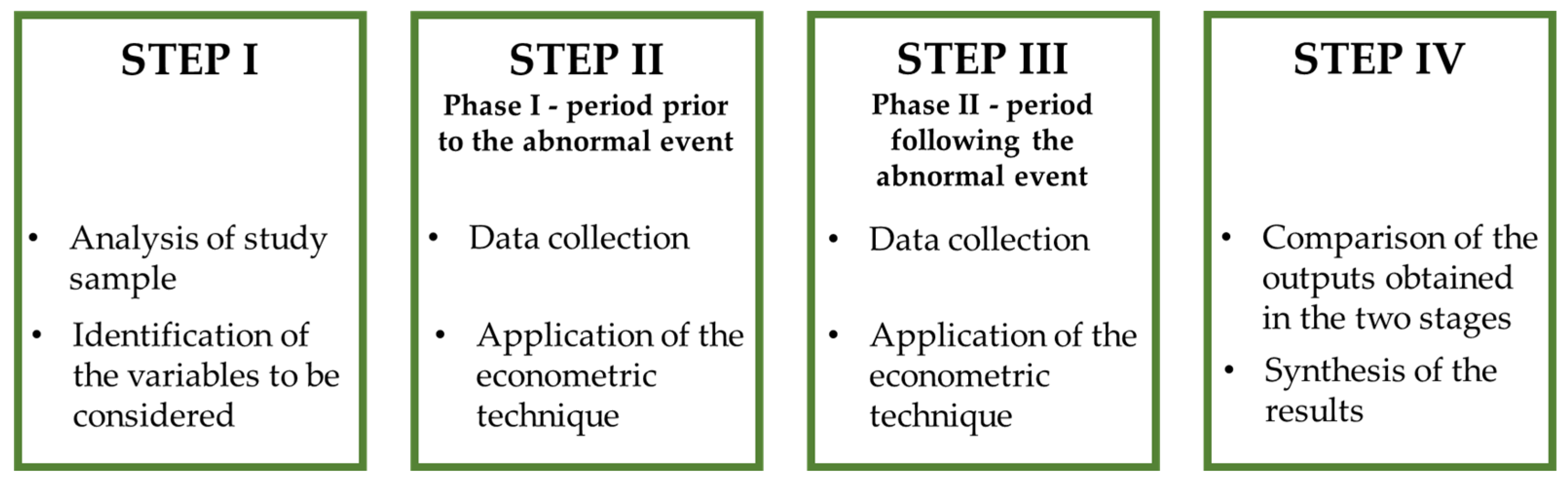
The dynamics of the real estate market can be influenced by many different socio-economic, political and geographical factors. To choose a methodology able of monitoring the residential market demand and of identifying likely variations caused by anomalous events, an analysis of the existing literature has been carried out to examine the main methods and techniques adopted to assess the effects of anomalous events on residential market appreciations.

An anomalous event, like the COVID-19 pandemic, is defined as an unexpected exogenous shock which is difficult to predict and impacts the real estate market [23], or marks a moment of strong discontinuity at a social and economic level [24].

In the international context, numerous contributions have aimed to assess the impacts of different anomalous events on the real estate market. These studies are heterogeneous, both in terms of the method used and their aim.

In the present study, anomalous events have been distinguished into (i) events with microeconomic effects, e.g., hurricanes, earthquakes, environmental disasters, and terrorist attacks, (ii) events with macroeconomic effects, e.g., global economic crises, pandemics, wars.

In the definition of the methods for the assessment of the anomalous events’ effects on the real estate market, it is fundamental to distinguish transitory consequences from permanent ones [24]. An anomalous event can affect the local economy in multiple ways: temporarily or permanently by (i) reducing companies’ productivity, (ii) damaging or destroying productive capital or (iii) interrupting supply chains. Several studies have investigated the influence of climate change, the frequency and intensity of precipitation and the increase in exposure to natural disasters on economic growth [25,26,27,28,29,30], both by analyzing the changes in selling prices and in rent [31]. For example, through the analysis of historical series of economic data, it has been estimated that in the United States, over ninety years (1920–2010), the effects of disastrous events of high magnitude have contributed to a decrease in housing prices of 2.5% and of rental fees by 5%, in the year following the event [31].

Among the several phenomena that can strongly and suddenly influence housing market dynamics, an earthquake can be considered an unexpected and exogenous event that can radically change the market. It is an exogenous risk factor, related to the specific city location, and its risk should be capitalized in housing prices [32].

The studies carried out on the real estate market in Japan, a country with high seismic risk, have demonstrated that the hedonic price method allows the risk perception both on the cost of land [33] and on housing rents [34] to be studied. This method ordinarily assesses market value by taking into account its intrinsic and extrinsic characteristics, and identifying the weight of each individual factor that contributes to the price conformation [35]. In the case of assessments linked to seismic events, the hedonic price method is used to verify the specific contribution of the seismic risk of the area on which the building is located, the property structural resistance, and the probability of occurrence of the harmful event [36,37].

In line with empirical intuition, the decrease in selling prices of a property located in an area subject to earthquakes is significantly higher immediately after the seismic event. This is because buyers tend to underestimate the risk if a recent event has not occurred [32].

In general, among the methods to assess the effects of an anomalous event on selling prices, the hedonic price method is widespread [32,36,37,38]. Furthermore, different studies have used the hedonic pricing method to measure willingness to pay (WTP) to avoid the consequences of natural disasters such as floods [39]. For example, the technique has been implemented to examine whether home owners change their subjective assessments of earthquake risk following the occurrence of a major seismic event. This method has often been integrated with the difference-in-difference (DD) technique, which allows the impact of an ‘unobserved’ variable, such as the consequences of an anomalous event, to be assessed on a chosen set of variables. In this sense, the DD method allows an assessment of the level of information of the population on a given risk, and the extent to which this affects the dynamics of the residential property market. In fact, if the population is informed about the consequences of a seismic or a meteorological event, the residential real estate market suffers the effects of an overestimation of the damage resulting from the event, with effects on selling prices [23,36,40,41,42]. Specifically, Belasen and Polachek [23], and Kim [42] have applied this technique to identify and quantify the effects of hurricanes in the USA residential market, and Rehse et al., 2019 [43] have used it for estimating the effects of environmental disasters of various natures. Keskin et al. [44], instead, have implemented a multilevel approach, capable of integrating several techniques simultaneously, to obtain a more effective assessment of the earthquake effects on the real estate market. On the other hand, Kinoshita (2020) [45] has described the use of conjoint analysis to evaluate the effects of an earthquake, with particular reference to the behavior and energy habits of communities.

Regarding the quantification of terrorist event effects on real estate dynamics, some studies have focused on the presence of subjective fear in the population and the consequent changes in housing choices. In particular, Caputo [46,47] and Anand [48] have examined the importance of the influence of the potential buyers’ psychological aspects on the markets, by defining the “regret theory”, where regret is defined as the fear of investors to repent their investment decisions. By comparing data before and after the terrorist event, it has been possible to observe that subjective fear and the perception of risk are factor able to modify the market trend and the balance in urban dynamics [49,50]. Abadie [51] has analyzed vacancy rates data to investigate the impact of an increased perception of terrorist risk, after 11 September 2001, on the office real estate market in downtown Chicago. Similarly, Kinoshita [45] and Morita [52] have found that the housing mechanisms following a terrorist event are strongly influenced by the level of perceived terrorist risk, both by operators and the population.

In addition, the short-term effects of an economic crisis have often been estimated using a technique borrowed from dynamics theory, called the impulse response function. On the basis of a stable system, this technique calculates the effects that could occur due to a perturbation coming from outside the system, but which has caused direct effects on one or more variables of the system [53]. For these analyses, the vector auto-regressive model (VAR) has been used [54,55,56,57]. Moreover, to investigate the effects of economic crises over time, predictive techniques based on regression analysis of time series have often been applied [58,59,60,61].

The consequences of the COVID-19 pandemic on the real estate market have been investigated using some of the different techniques mentioned above [62]. In particular, Wang et al. used a DD approach to analyze the variation on housing prices with reference to five areas of the United States of America (USA) [63], and Li and Zhang have studied the spatial distribution of housing price changes in the USA implementing a statistical analysis of 2856 U.S. counties’ data [64]. The COVID-19 pandemic triggered a global economic crisis in all sectors [65], comparable in intensity and magnitude of consequence to the major economic crises of the last hundred years [66], i.e., the Oil Shock (1972–1976), the First Debt Crisis in Italy (1982–1986), the European Monetary System Crisis (1992–1996), the attack on the Twin Towers in America (2001–2004), and the “Sub-prime” Global Financial Crisis (2008–2013). Therefore, the pandemic can be considered an exogenous shock to the housing market [57].

3. Methodology

With regard to the aims of the present research and to the framework defined in the literature review, the methodology proposed intends to provide an operational approach for the assessment of effects of anomalous events on the housing market, and is articulated into four steps. The operating practice to be implemented in each phase is illustrated below, and the stages carried out in this research are described with reference to the selected case study.

The first step (Step I) concerns the analysis of study sample, i.e., in the specific case, the investigation of the six Italian cities selected and of the most influencing factors on the residential market phenomena, in order to identify the variables to be considered in the model.

In the second step (Step II) a study sample related to residential properties sold in the period prior to the anomalous event was collected for the investigation of the “ordinary” market mechanism. Therefore, with reference to the present analysis, a sample of 165 housing properties for each city sold in the second half of 2019 (Phase I: “pre-COVID-19 pandemic”) was detected. For each data set, some preliminary correlation analysis and descriptive statistic examinations were carried out for the monitoring of data samples statistical robustness. (Tables S1–S24 in the Supplementary files, respectively). Then, an econometric technique was implemented in order to obtain a function for each city able to identify the main relationships between the factor selected and the selling prices.

The third step (Step III) refers to the same logical approach carried out in the second step with reference to the Phase I, by detecting data related to the period following the occurrence of the phenomenon. In the specific case, the study samples were related to the six Italian cities selected for the analysis, with reference to the first half of 2021 (Phase II: “COVID-19 pandemic in progress”).

In the fourth step (Step IV) the comparison of the outputs obtained in the two stages (Phases I and II) is performed. Thus, the synthesis of the results was developed in order to (i) identify the variations in the residential market demand deriving from the COVID-19 pandemic arising and (ii) to provide a framework for orienting the planning and design decisions.

In Figure 1, a summary of the main steps for the implementation of the methodology proposed is reported.

4. Case Study

4.1. Implementing Step I of the Methodology

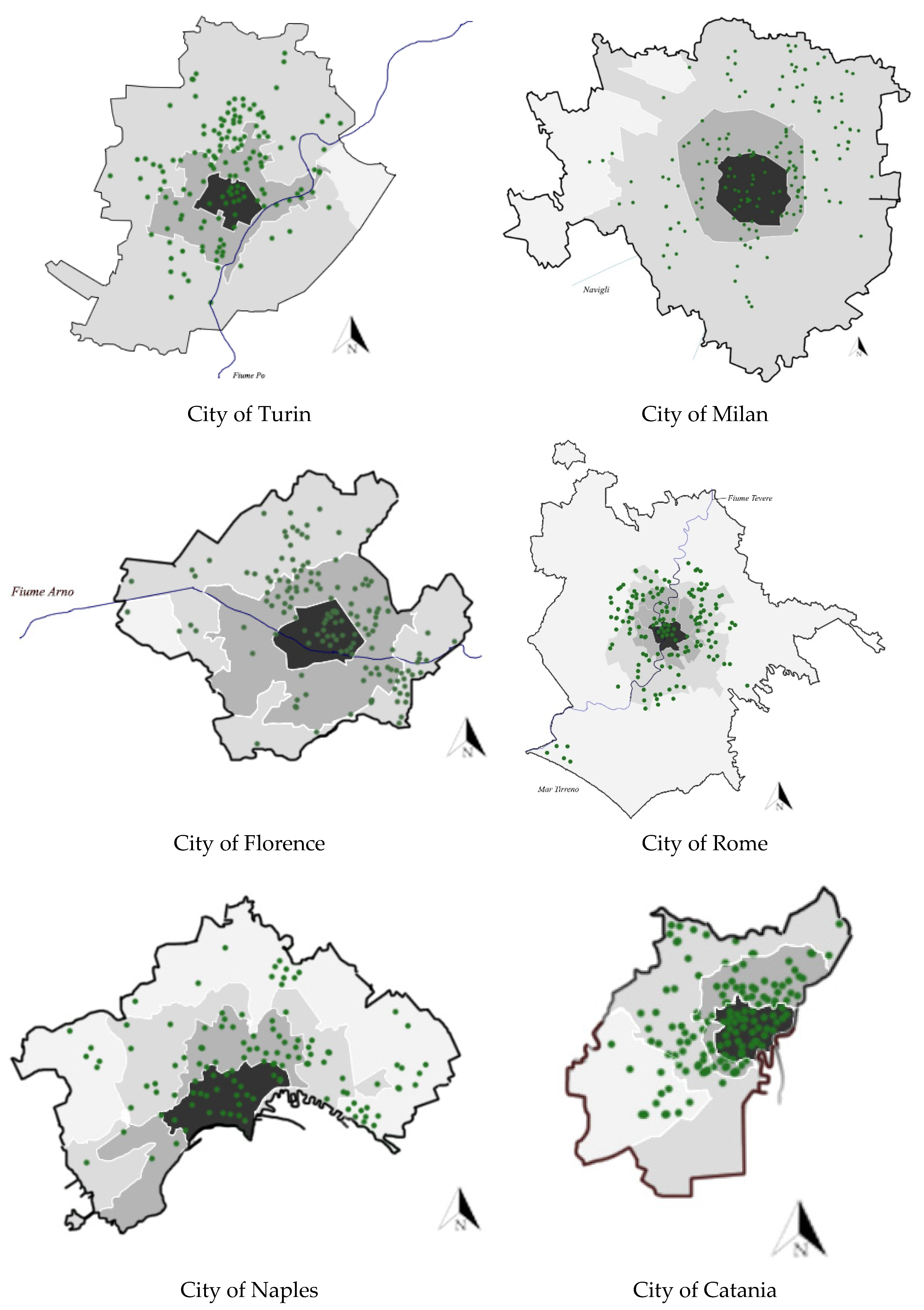
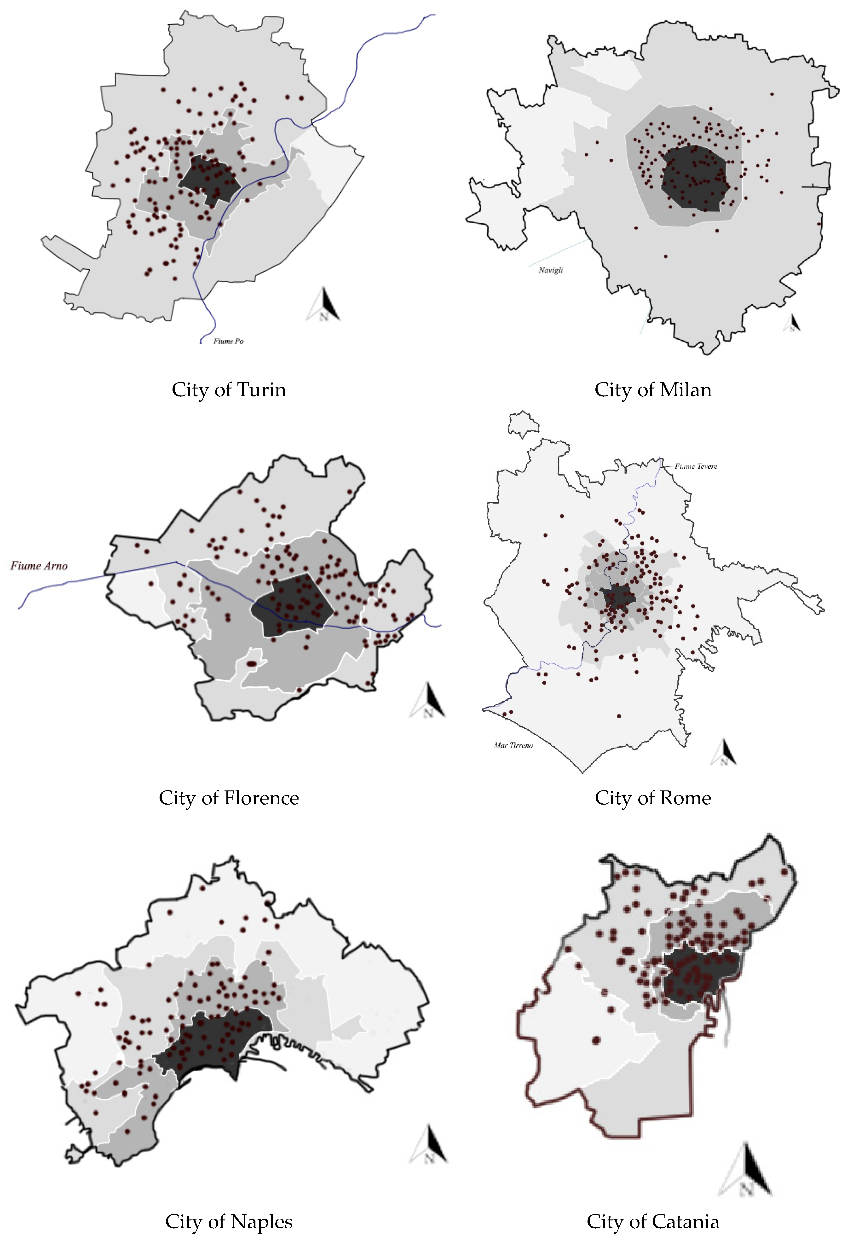
4.1.1. The Study Samples

In order to assess the changes occurred in the Italian residential market, the six largest Italian metropolitan cities were selected: Milan and Turin for Northern Italy, Rome and Florence for Central Italy, and Naples and Catania for Southern Italy and the Islands. For each city, the main social, urban, economic and demographic factors were investigated in order to understand the context of reference for each city. In

Table 1. Main distinctive features for each Italian city considered in the analysis.

Factor	Turin	Milan	Florence	Rome	Naples	Catania
Number of inhabitants (n.)	870,952	1,396,059	372,038	2,837,332	962,589	311,402
Surface (km2)	130.01	181.67	102.32	1287.36	119.02	182.90
Population density (inhabitant/km2)	6699.12	7684.59	3636.02	2203.99	8087.62	1702.58
Old age index	204.10	196.30	220.40	162.60	114.40	139.60
Square meters per occupant in occupied residential units (m2)	41.00	41.50	41.40	29.40	31.70	37.10
Number of residential buildings (n.)	36,158	42,980	31,070	137,021	40,755	28,988
Empty residential properties (n.)	36,779	37,073	5164	118,531	14,140	28,567
Per capita income (€)	25,015	34,046	26,503	28,241	22,434	20,179

Source: elaborations of the authors on ISTAT database.

, a summary of the distinctive features for each city is reported [67].

As can be seen in Figure 2 and Figure 3, for each city two study samples consisting of 165 housing properties were detected. The first concerned 165 residential units sold in the second half of 2019 (Phase I), whereas the second related to 165 residential units sold in the first of 2021 (Phase II). In Figure 2, the locations of the properties (green points) collected for the cities in the pre-COVID-19 spread are represented, and it is possible to note their heterogeneous distribution throughout the urbanized territory. The entire sample was detected in order to take into account all municipal trade areas provided by the Real Estate Market Observatory (OMI) of the Italian Revenue Agency, i.e., the “portion of the territorial band that reflects a homogeneous part of the local real estate market, in which there is a substantial uniformity of appreciation for economic and socio-environmental conditions is observed” [68] or, the central, semi-central, peripheral and suburban portion of urbanized territory that synthetized the features of the neighborhood. The same considerations were carried out for Figure 3, pertaining to the locations of the properties (red points) that refer to the sample of Phase II.

Some issues could be developed regarding the sizes of the data samples; however, even if though they were not large, they were certainly interesting compared with other Italian mass appraisal applications, taking into account the structural opacity that generally characterizes the Italian real estate market. In this sense, the sample size used by Simonotti [69], constituted by 33 pieces of data, the research carried out by Curto [70] that considered a sample of 66 individuals, the study of Del Giudice & De Paola [71] with a sample of 64 data, and the work of D’Amato [72] that implements a sample constituting of 114 individuals, could be mentioned. Moreover, it should be highlighted that the sizes of the data samples collected for each city satisfied the “rule-of-thumb” recognized in the current literature [73]: after establishing that N is the number of subjects in each data sample and m is the number of influencing factors considered, the rule states that N ≥ 50 + 8m must be required for multiple correlation, and N ≥ 104 + m for partial correlation.

For each property, the total selling price and the intrinsic factors were detected, on the basis of (i) the aim of the research focalized to investigate likely changes in the housing market demand, (ii) the indications provided by the market operators in the area, (iii) the data generated by the Observatory of the Real Estate Market (OMI) of the Italian Revenue Agency [68], (iv) the urban morphological and social examination of each city, taken into account in the negotiation phases by local operators (sellers and buyers) [74,75]. Furthermore, the localization of each residential unit in the context of each Italian city, according to the OMI, has been included.

4.1.2. Variables

For the definition of the model able to identify the most influencing factors on housing prices in the two phases considered in the analysis, the dependent variable is represented by the total selling price (Q), expressed in € (euro).

The independent variables were chosen according to the analysis of current literature, considering the specific indications supplied by the market operators in the area, i.e., real estate agents, as the main property characteristics considered in the bargaining phases by sellers and potential buyers [76]. The variables considered in the study are illustrated in

Table 2. Variables selected in the analysis.

Category	Acronym	Denomination	Description	Measurement Unit	Variable Typology	References
Surfaces	Si	Internal area	Internal surface of the property	m2	Quantitative continuous	[77,78,79,80]
	Sb	Surface of balconies or terraces	Net external surface of balconies or terraces directly accessible from the property.	m2	Quantitative continuous	[80,81]
	Sg	Surface of private garden	Net external surface of gardens directly accessible from the property.	m2	Quantitative continuous	[77,82]
	Se	Presence of condominium areas	External surfaces accessible from the condominium areas of the building and not for the exclusive use of the property.	-	Dummy (1 or 0)	[82]
Maintenance conditions of the property	Me	Excellent	The “excellent” state are related to properties characterized by high construction and aesthetic quality.	-	Dummy (1 or 0)	[78,80,82]
	Mg	Good	The “good” state refers to properties whose maintenance conditions are acceptable and whose functions can be carried out without heavy refurbishment interventions.	-	Dummy (1 or 0)
	Mp	Poor	The “poor” state refers to properties whose maintenance conditions are not acceptable and heavy refurbishment interventions are needed.	-	Dummy (1 or 0)
Internal services	B	Number of bathrooms	Number of toilets for the exclusive use of the property.	n.	Quantitative discrete	[77,78,79,80]
Localization in the building	L	Floor level	Floor level on which the property is located.	n.	Quantitative discrete	[77,79]
Building age	Yc	Building construction year	Construction year of the building within which the residential unit is located. The variable is assessed as the difference between the year 2019 (Phase I) or 2021 (Phase II) and the construction year.	n.	Quantitative continuous	[77,79]
Municipal trade area	C	Central	Municipal trade area in which the property is located according to the geographical distribution developed by the Real Estate Market Observatory (OMI) of the Italian Revenue Agency.	-	Dummy (1 or 0)	[83,84]
	Sc	Semi-central		-	Dummy (1 or 0)
	P	Peripheral		-	Dummy (1 or 0)
	Sub	Suburban		-	Dummy (1 or 0)
OMI quotation	Vm	Average market value	Average quotation between the maximum value and the minimum value for civil properties determined for the Phase I (“pre-COVID-19 pandemic”) and the Phase II (“COVID-19 pandemic in progress”) by consulting the Real Estate Market Observatory (OMI) of the Italian Revenue Agency.	€	Quantitative continuous	[84]

.

For each explanatory variable, the category of which each belongs, the acronym, the full denomination, a brief description, the measurement unit and typology of the variable (dummy or quantitative) are specified.

4.2. Implementing Step II of the Methodology

The Step II of the methodology proposed assessed the housing market demand concerns the year 2019, i.e., Phase I: “pre-COVID-19 pandemic”.

In this sense, 990 residential properties (165 for study sample related to each Italian cities considered) were collected. Figure 4 reports a summary description of the main operations of the Step II to be implemented. It should be noted that the operations illustrated for Phase I were replicated for Phase II “COVID-19 pandemic in progress”. The outputs obtained by the comparison of the results related to the two phases will verify possible changes in some specific market factors appreciations.

The data, i.e., the values of the selected explanatory variables relating to each property of the six study samples in both phases, were subsequently homogenized through a normalization operation in order to obtain the numerical terms of the same size order, and to facilitate the comparison between them.

Tables S1–S6 in the Supplementary Materials report the main descriptive statistics of the selling prices and values of the explanatory variables for the six Italian cities selected and for the two phases analyzed (Phases I and II). The investigation has allowed a global reading of the phenomenon through the chosen samples. For each characteristic, the recorded average value, the standard deviation, the different levels or intervals that each variable can be divided into and the frequencies with which each was verified for the properties of the study samples, are reported. Furthermore, to monitor the representativeness of the study samples, some data included in the ISTAT database [67] referring to the Italian municipalities, were examined. According to the analysis carried out for Phase I, the samples were statistically performing, and the differentials with the ISTAT database for the characteristics compared were low.

4.2.1. Econometric Technique

The econometric technique used is named Evolutionary Polynomial Regression (EPR-MOGA). It combines the characteristics of a regression numerical system with the genetic programming technique, by applying a multi-objective evolutionary genetic algorithm, as an optimization strategy based on the Pareto frontier. This technique is able to identify, among the variables affected by the analysis, both simple functional relationships (such as log-linear) and more complex functional relationships, and therefore performs well from a statistical point of view [77,78,85,86].

After setting the dependent variable (Y) and n independent variables (Xn), the technique identifies the function (model Y = f(Xi)) whose polynomial expression is a combination of independent variables and numerical coefficients. The resulting model obtained by the EPR-MOGA implementation is able to satisfy a multi-objective Pareto frontier in terms of (i) maximizing of the statistical accuracy of the model; (ii) minimization of the number of polynomial coefficients; and (iii) minimization of the number of inputs for each variable [85].

The generic expression of the models generated by EPR-MOGA is summarized by Equation (1):

$$Y=a_0+{\displaystyle \sum _{i=1}^n[a_i\cdot {(X_1)}^{(i,1)}\cdot \dots \cdot {(X_j)}^{(i,j)}\cdot f({(X_1)}^{(i,j+1)}\cdot \dots \cdot {(X_j)}^{(i,2j)})]}$$

(1)

In particular:

• a₀ is the constant additive term, i.e., the bias;
• n is the number of additive terms, i.e., the length of the polynomial expression (constant additive term excluded);
• a_i is the numerical coefficient to be assessed for each additive term;
• X_i is the candidate explanatory variables to be selected by the model;
• (i, l)—with l = (1, …, 2j)—is the exponent of the l-th variable within the i-th additive term. It is selected by the technique among a set of possible exponents chosen by the user from a range of candidate real numbers;
• f is a function selected by the user from a set of candidate mathematical expression.

For each model returned by the technique, a series of indicators are calculated to immediately determine the statistical performance of the function which are expressed by the coefficient of determination (CoD), calculated as shown in Equation (2), where y_e are the values of the dependent variable assessed by the EPR technique, y_d are the collected values of the dependent variable, and N is the sample size.

$$\mathrm{CoD}=1-\frac{N-1}{N}\cdot \frac{{\displaystyle \sum _N{(y_e-y_d)}^2}}{{\displaystyle \sum _N{(y_d-mean(y_d))}^2}}$$

(2)

The CoD varies from the value 0 (minimum statistical accuracy) to the value 1 (maximum statistical accuracy). In particular, the fitting of each model is higher when the CoD is close to the unit value, by confirming the model structure suitability to represent the overall observed dataset. Therefore, the model that best satisfies the Pareto frontier is obtained, and the user can identify the most appropriate solution whose (i) CoD ensures a medium/high statistical robustness level, (ii) algebraic form is not too complicated to interpret, (iii) mathematical expression includes the largest number of variables considered capable to investigate the phenomenon addressed. This has often been used for analysis similar to that of the present research, regarding influencing factors in the market dynamics and the selling prices, or to identify the contribution of specific variables in the housing values formation processes [78,79,80,86,87,88], but never before to evaluate the effects of an extra-local exogenous event on the real estate market.

4.2.2. Application of the Technique to the Phase I: “Pre-COVID-19 Pandemic”

In order to define a model (price function) that could efficiently describe the selling price formation mechanism for each study sample related to the six Italian cities considered for Phase I, the EPR-MOGA technique was implemented with no function f, through a static regression, a maximum number of equation terms equal to eight and a set of candidate exponents belonging to the range (0, 0.5, 1, 2). The use of these exponents allows the model to consider the variable in its original form (exponent equal to 1), not to consider the variable (exponent equal to 0), to consider it elevated to the square (exponent equal to 2) and to make it the square root (exponent equal to 0.5). For all the samples, the dependent variable was represented by the natural logarithm of the selling price (Y = ln(P)), according to other relevant studies [81,82,89,90,91]. The log-linear model has been frequently implemented as it has different advantages [84,85,92,93], i.e., the partial mitigation of a common form of heteroskedasticity.

The implementation of the EPR-MOGA technique was iteratively applied six times (one for each study sample), without varying the settings chosen. It was preferable to obtain a model for each Italian city selected and then compare the outputs.

Every time that the EPR-MOGA was used, several models were generated, but only one for each of the six cities (6 total models) was chosen by the user, i.e., the operator who was implementing the technique and was carrying out the analysis, as reported in

Table 3. Models chosen from the EPR-MOGA implementation outputs for each Italian city analyzed.

City	Model	CoD (%)
Turin	Y = + 2.3105 · Vm0.5 − 0.39501 · Sc0.5 · Mg0.5 − 15.6167 · Yc2 · P2 · Mg0.5 + − 38.8898 · Sb0.5 · Yc · P2 · Me2 · Vm2 + 1.402 · Sb0.5 · B + 3.1882 · Si0.5 + 8.4518	81.48
Milan	Y = + 0.92925 · Vm0.5 − 2.1509 · Se0.5 · Yc0.5 − 0.72176 · Sb0.5 · Mg0.5 + 8.6914 · · Sb0.5 · B2 · Yc + 8.9345 · Si0.5 + 7.7893 · Si0.5 · Se2 · Yc − 5.0165 · Si + 9.146	66.44
Florence	Y = + 1.8883 · B0.5 · Vm − 2.3554 · B · Yc0.5 · Vm − 19.929 · Sg · Sb0.5 · Yc0.5 + + 2.2829 Si0.5 + 48.0618 · Si0.5 · Sg · Yc2 + 4.2736 · (Si + Sb + Sg)0.5 · L0.5 · Yc · Vm + + 2.3275 · (Si + Sb + Sg)0.5 · Sb0.5 · B0.5 · Me2 − 3.0961 · (Si + Sb + Sg) · Si · L0.5 · P 0.5 + + 10.5998	84.02
Rome	Y = + 2.0813 · Vm0.5 + 0.77051 · L0.5 · B · Me0.5 + 7.5564 · L0.5 · B2 · Yc + + 2833.437 · Sg ·L2 · Mg0.5 · Vm2 + 2.6857 · Si0.5 + 579.0223 · (Si + Sb + Sg)0.5 · Sb2 · L2 · B0.5 · C0.5 · Mg0.5 + 9.7199	86.23
Naples	Y = + 1.6557 · Sc0.5 · Me0.5 · Vm + 2.8709 · B0.5 · Vm0.5 + 4.2863 · Si0.5 − + 22.669 · Si · Yc2 · Mg0.5 + 75.9095 · Si2 · L0.5 · Yc · P0.5 + 9.1516	83.13
Catania	Y = − 0.85036 · Yc0.5 + 0.90016 · L0.5 · Sc2 · Me0.5 + 8.2726 · L · Yc2 · C2 · Vm0.5 + + 3.147 · Sb0.5 · B · Vm + 25.5332 · Sb · Se · L0.5 + 2.6756 · Si0.5 − 9880.7007 · Si2 · · Sb2 · Se0.5 · L2 · Vm0.5 + 10.2077	74.08

. For each of them, the statistical accuracy of the outputs, or the CoD, was specified.

Firstly, it should be observed that each equation was characterized by a high statistical accuracy level (CoD = +81.48% for the city of Turin model, +66.44% for the model related to the city of Milan, +84.02% for the city of Florence, +86.23% for the city of Rome equation, +83.13% for the city of Naples, +74.08% for the model selected for the city of Catania) and included a large number of influential factors (nine for the cities of Turin, Florence and Rome, seven for the Milan sample, and ten for the cities of Naples and Catania).

The main statistical performance indicators—the root mean square error (RMSE), the mean absolute percentage error (MAPE), and the maximum absolute percentage error (MaxAPE)—showed a good statistical reliability of the models. The lowest RMSE concerned the city of Florence (3.58%) and the highest referred to the city Milan (4.51%); furthermore, the lowest MAPE was calculated for the Rome study sample (2.80%), and the highest MAPE results were for the city of Milan (3.12%). Moreover, the city of Rome presented the highest MaxAPE (9.42%). The lowest MaxAPE was verified for the Catania case study (8.24%).

In order to verify the stability of the models obtained, a ten-fold cross-validation [86,94] was implemented on the starting database for each model. The outputs obtained (

Table 4. Average percentage errors (%) obtained through a ten-fold cross-validation.

No. Iteration	Turin		Milan		Florence		Rome		Naples		Catania
	Training Set	Validation Set	Training Set	Validation Set	Training Set	Validation Set	Training Set	Validation Set	Training Set	Validation Set	Training Set	Validation Set
Iteration 1	2.121	2.235	2.899	2.899	2.196	2.318	2.121	2.121	2.256	2.256	3.801	3.821
Iteration 2	2.845	2.922	3.584	3.584	2.845	2.845	2.845	2.845	2.845	2.845	3.125	3.225
Iteration 3	2.058	2.134	2.889	2.889	2.058	2.058	2.058	2.058	2.665	2.665	3.004	3.087
Iteration 4	2.329	3.120	2.789	2.789	2.329	2.329	2.329	2.329	2.015	2.015	2.997	3.102
Iteration 5	2.279	3.089	3.256	3.256	2.279	2.279	3.345	3.345	2.058	2.058	2.279	2.279
Iteration 6	2.228	3.310	3.658	3.658	2.228	2.228	2.228	2.228	2.987	2.987	2.228	2.228
Iteration 7	3.123	3.531	3.987	3.987	3.123	3.123	3.004	3.004	2.753	2.753	3.123	3.123
Iteration 8	2.127	2.178	3.854	3.854	2.127	2.127	2.127	2.127	2.861	2.861	2.127	2.127
Iteration 9	3.404	3.650	3.145	3.145	3.404	3.404	2.767	2.767	2.001	2.001	3.404	3.404
Iteration 10	2.026	2.077	3.521	3.521	2.026	2.026	2.026	2.198	3.021	3.021	2.026	2.026

) confirmed the good prediction performance of the functional models obtained for each city.

In

Table 5. Variables selected by the models generated by EPR-MOGA for each study sample of Phase I.

No.	City	N. Variables	Si	Sg	Sb	Se	L	B	Yc	C	Sc	P	Mg	Me	Vm
1	Turin	9	✓		✓			✓	✓		✓	✓	✓	✓	✓
2	Milan	7	✓		✓	✓		✓	✓				✓		✓
3	Florence	9	✓	✓	✓		✓	✓	✓			✓		✓	✓
4	Rome	10	✓	✓	✓		✓	✓	✓	✓			✓	✓	✓
5	Naples	9	✓				✓	✓	✓		✓	✓	✓	✓	✓
6	Catania	10	✓		✓	✓	✓	✓	✓	✓	✓			✓	✓

a summary of the variables selected in each model is shown to conveniently compare the most influencing factors among those analyzed.

It should be noted that the variables referring to the internal area (Si), the number of bathrooms in the property (B), the building construction year (Yc) and the average market value (Vm) were present in all six equations, with a non-zero multiplicative coefficient. Furthermore, no variable was excluded by the models and all factors analyzed were included in at least two models.

For all the equations obtained for Phase I, their algebraic structure did not allow an immediate interpretation of the functional relationships among the variables, as each additive term was a combination of different variables that occurred several times in the same model. Therefore, in order to verify the empirical consistence of the functional links between the independent explanatory variables selected by each model, and the values of the dependent variable of total selling prices, a simplified exogenous approach that considered the other variable values equal to the average values of the starting database (value “1” or “0” if the factor was a dummy variable) was used. This approach determined the marginal price of the generic variable through the changes in value of the assessed variations of selling prices, in correspondence with each i-th variable in the admissible range of its corresponding sample collected. In particular, for each Italian city, with reference to the Phase I (second half of 2019 “pre-COVID-19 pandemic”) Figures S1–S6 in the Supplementary Materials show the functional correlations detected for each explanatory variable selected by the six models.

The marginal influence on selling prices, in terms of the average percentage variation obtained in correspondence with the passage from one level to the next, or from the absence to the presence of a specific factor, was reported for each variable. The analysis of the functional correlations between independent explanatory variables, selected by the models and housing prices, verified the empirical evidence of the coefficient signs for all the cities, as the consistency of the links with the expected phenomena was confirmed.

According to the aim of the research, some interest can be accomplished for the intrinsic factors analyzed, connected with the domestic spaces and their related accessory surfaces:

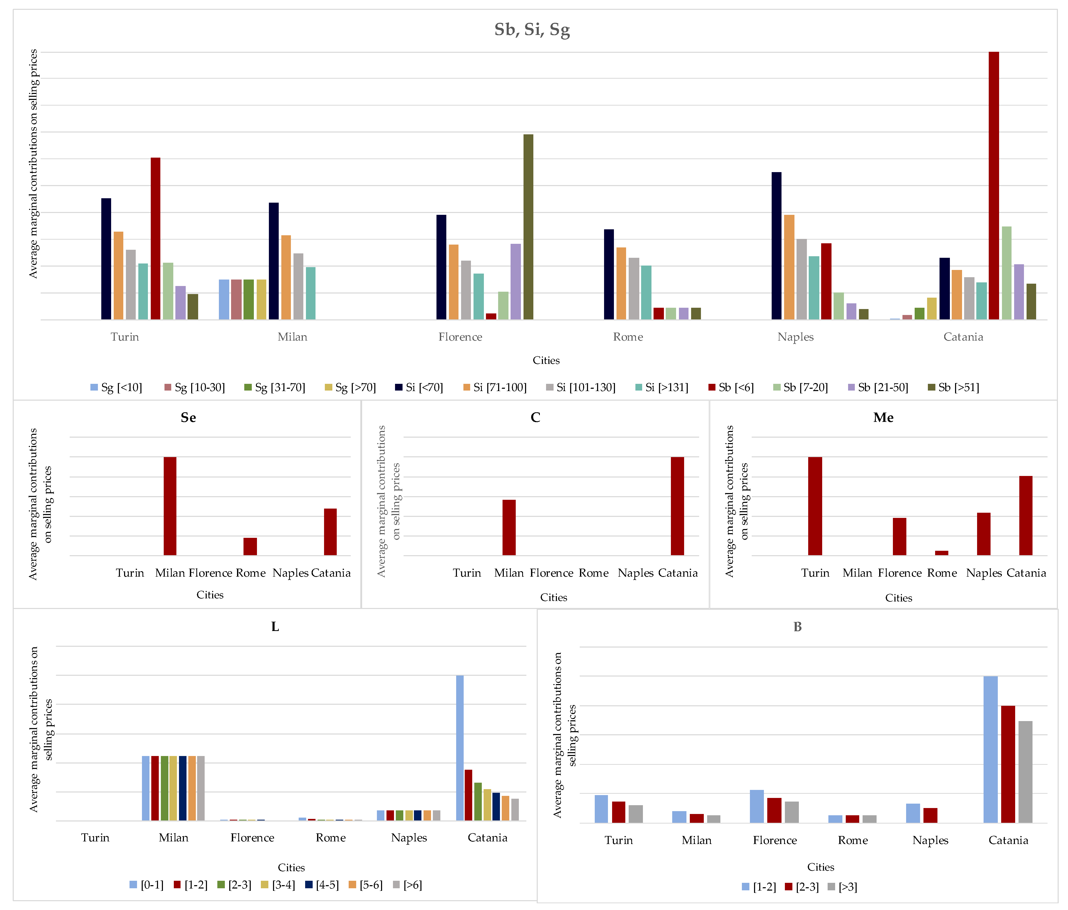
• A direct link between the internal surface and housing prices was detected for the six cities considered (+26% for the city of Turin, +37% for the city of Milan, +20% for the city of Florence, +38% for the city of Naples, +25% for the city of Rome, and + 6% for the city of Catania, considering an average variation of 40 m²).
• Variables related to direct and private accessory surfaces, i.e., balconies or terraces and gardens, had different influences; for example, for the city of Turin the presence of balconies was strongly appreciated up to a surface of 9.50 m² (+22%), beyond which the contribution on the prices progressively decreased (an average +5%). The marginal contribution on selling prices provided by the biggest balconies or terraces and gardens surfaces was confirmed by the microeconomics principle, for which the relevance of a good was strongly associated with the need of it (known as law of decreasing marginal utility). Moreover, the variable was also directly linked to the selling prices in the city of Milan, for which the variation between the absence and the presence of balconies was higher (+14%), compared with the subsequent balconies area (+4%). The model selected for the city of Florence proved a growth of the residential values in correspondence with the presence of balconies (+31% compared with its absence), and a progressive attenuation in prices increase for larger balcony surface areas (+17%). Similarly, for the city of Catania, a direct correlation between the variable related to the surface of balconies Sb and housing prices was found, with a relevant initial variation equal to +19% between the properties without balconies and those characterized by the balcony presence. Then, the percentage variation decreased, and was equal on average to +4%. The presence of private gardens was not included in the models of the city of Turin, Naples, Catania and Milan, due to the most common residential typology sold in those markets, i.e., residential units located in apartment buildings. A decrease in housing prices was found for the city of Florence model (−11%), in correspondence with properties with private gardens. With reference to the study sample collected, only 6% of the total individuals included were characterized by this domestic space, and all were localized in the higher hydrogeological risk areas of the city. Furthermore, a significant influence of private green area was detected for the city of Rome, especially due to the position of the sample residential units, in particular, valued urban zones (in the proximity of the Appia Antica Regional Park).
• The models selected showed a lack of appreciation for the presence of condominium areas, in the second half of 2019, in the cites of Naples, Turin, Florence and Rome. On the other hand, the price functions generated by the EPR-MOGA technique for the cities of Catania and Milan denoted a relevant contribution—positive for the first city, negative for the second—deriving from the presence of these spaces on selling prices. In particular, for the city of Catania, it should be outlined that most properties collected in the study sample were located in prestigious residential complexes, in which the shared gardens were in excellent conservative conditions, and were for the exclusive use of inhabitants. On the other hand, for the city of Milan, most residential units in the study samples considered for the external condominium area (41% of the total sample individuals) were constituted by economic buildings, for which other factors could negatively influence the selling prices.
• The floor level on which each residential property was located influenced the housing dynamics in the cities of Florence, Rome, Naples and Catania. The model selected for the city of Naples indicated an average variation on selling prices equal to +7%, and a higher significance in correspondence with the passage from the ground floor to the first floor (+25%), and an attenuation for the highest floors, from level eight upward (+5%). For the city of Catania, a direct functional correlation was found on average equal to +2%, and a relevant appreciation for the ground floor was detected, if the properties were characterized by condominium areas, compared with the higher floors. The same positive link typology was revealed with regards to the study sample collected for the city of Rome, for which the highest floor levels were those most appreciated, compared with the lowest ones. In addition, in the central trade area, the location on the highest floors allowed panoramic views that implied a strong influence on housing values. A moderate contribution on selling prices was observed for the city of Florence, with a marginal price equal to 4%.
• The central municipal trade area variable was included in the models selected for the cities of Rome and Catania; the semi-central areas appeared in the models of the cities of Turin, Catania and Naples, and the peripheral area factor was also present in the price functions of Turin, Florence and Naples. It should be outlined that the semi-central municipal trade area was particularly appreciated in the context of the city of Naples (+25%) and in the city of Catania (+52%), whereas a negative influence was given by the position of housing properties in the semi-central trade area and peripheral area of the city of Turin (−33% and −38%, respectively). In the city of Florence, the selling price variation determined by the localization of the property in the peripheral area was equal to –18%, whereas for the city of Naples a decrease in housing prices equal to –20% was recorded for the peripheral trade area. The location of properties in the central municipal trade area of the city of Rome determined an increase in selling price equal to +13%, whereas this was equal to +5% in the central area of Catania.

4.3. Implementating Step III of the Methodology

Application of the Technique to Phase II: “COVID-19 Pandemic in Progress”

By recalling the aim of the present research, the identification of the changes in residential market demand caused by the COVID-19 pandemic in six Italian metropolitan cities, Step III of the analysis concerns the same operative logic carried out as in the previous Step II. Therefore, six study samples, each consisting of 165 housing properties sold in the first half of 2021 (one for each city) were collected. For each residential unit, the same factors detected for Phase I were investigated in order to determine the most influential factors on selling prices, and to study the functional correlation between the explanatory independent variables and price. Thus, the same stages developed in Phase I (second half of 2019) were replicated in Phase II (first half of 2021).

The implementation of the EPR-MOGA technique was iteratively carried out for all the samples. The dependent variable of total selling price was constituted by its natural logarithm (Y = ln(Q)). The application of EPR-MOGA generated several models able to describe the residential market dynamics, and those chosen for the analysis of the functional link between influential factors and housing prices are reported in

Table 6. Models generated by the EPR-MOGA implementation for each Italian city analyzed for the Phase II.

City	Model	CoD (%)
Turin	Y = + 2.434 · Vm0.5 + 0.3733 · Me0.5 + 0.99371 · Sb0.5 · B0.5 · Vm0.5 − + 4.4136 · Sb0.5 · B0.5 · Yc0.5 · P0.5 · Me0.5 + 7.617 · Si0.5 − 4.1752 · Si · Vm0.5 + + 7.4833	85.53
Milan	Y = + 0.49351 · C0.5 · Vm − 0.88769 · Yc0.5 · P − 0.56312 · L0.5 · B0.5 · Mg + + 24.1533 · Sg0.5 · Se2 · L + 1.2286 · Sg · Vm + 8.1673 · Si0.5 − 4.1711 · Si + + 2.8284 · Si · L · B0.5 + 10.7489	96.04
Florence	Y = + 23.2683 · Vm0.5 − 13.2187 · Vm + 0.61728 · B0.5 · Me 0.5 · Vm2 + + 1.8377 · Sb2 + 5.8364 · Si0.5 + 170.3596 · Si0.5 · Sb2 · L · Yc − + 2.2608 · Si + 0.18337	93.00
Rome	Y = + 2.3773 · Vm0.5 + 0.27166 · Me − 0.66914 · Yc0.5 · Me2 + + 9.5008 · Se · Yc2 · P2 + 1.7449 · Sb · L0.5 · B + 3.0846 · Si0.5 + + 2.5818 · Si0.5 · L0.5 · Yc2 · Me2 + 9.402	89.84
Naples	Y = + 4.3382 · Vm − 2.0486 · Vm2 + 0.98283 · L · Yc0.5 · Me2 + 0.75291 · Sb0.5 · B0.5 · · Me0.5 + 9.3479 · Si0.5 − 4.2403 · Si + 7.4542	93.72
Catania	Y = + 1.9795 · Vm0.5 + 0.38123 · Me2 + 1.0016 · B0.5 + 13.2376 · L0.5 · B2 · Yc2 · Mg + + 2.5865 · Sb0.5 · Se2 · B · Yc · C · Me2 + 2.1141 · Sg2 · Yc0.5 · Vm2 + 2.762 · Si0.5 + + 8.1768	84.73

.

For each polynomial equation, the CoD was specified; in particular, a high statistical accuracy level was associated with them (+85.53% for the city of Turin, +96.04% for Milan, +93.00% for Florence, +89.84% for the city of Rome, +93.72% for Naples, +84.73% for Catania).

Moreover, in this analysis the main statistical indicators (RMSE, MAPE and MaxAPE) were calculated, and a ten-fold cross-validation was carried out. With reference to the statistical indicator the lowest RMSE was concerned with the city of Milan (3.21%) and the highest referred to the city Turin (3.98%). Furthermore, the lowest MAPE was calculated for the Milan study sample (2.80%), and the highest MAPE was calculated for the city of Catania (3.78%). Moreover, the city of Catania presented the highest MaxAPE (9.21%), and the lowest MaxAPE was verified for the Florence case study (8.12%).

Table 7. Average percentage errors (%) obtained through a ten-fold cross-validation for Phase II.

No. Iteration	Turin		Milan		Florence		Rome		Naples		Catania
	Training Set	Validation Set	Training Set	Validation Set	Training Set	Validation Set	Training Set	Validation Set	Training Set	Validation Set	Training Set	Validation Set
Iteration 1	2.217	2.351	2.551	2.614	2.292	2.434	2.227	2.237	2.125	2.136	2.660	2.667
Iteration 2	2.872	2.889	2.121	2.179	2.880	2.887	2.917	2.938	2.884	2.894	3.201	3.212
Iteration 3	2.091	2.078	2.889	2.985	3.210	3.221	2.156	2.208	2.485	2.506	2.998	3.008
Iteration 4	2.373	2.348	2.789	2.843	2.384	2.394	2.385	2.448	2.444	2.496	2.581	2.602
Iteration 5	2.299	2.364	3.256	3.258	2.309	2.330	3.345	3.403	2.252	2.315	2.411	2.463
Iteration 6	2.247	2.231	2.543	2.653	2.268	2.320	2.273	2.369	2.987	3.045	3.012	3.075
Iteration 7	3.208	3.138	2.852	2.985	3.260	3.323	3.004	3.058	2.101	2.197	2.589	2.647
Iteration 8	2.130	2.129	2.998	2.895	2.193	2.251	2.184	2.186	2.001	2.055	2.875	2.971
Iteration 9	3.201	3.321	3.145	3.145	3.259	3.355	2.767	2.782	2.589	2.591	3.001	3.055
Iteration 10	2.028	2.080	3.521	3.521	2.124	2.178	2.049	2.198	3.021	3.036	2.498	2.500

reports the output of the ten-fold cross-validation. These analyses confirmed that the selected samples were stable and statistically performing.

In

Table 8. Variables selected by the models generated by EPR-MOGA for each study sample for Phase II.

No.	City	N. Variables	Si	Sg	Sb	Se	L	B	Yc	C	Sc	P	Mg	Me	Vm
1	Turin	7	✓		✓			✓	✓			✓		✓	✓
2	Milan	10	✓	✓		✓	✓	✓	✓	✓		✓	✓		✓
3	Florence	7	✓		✓		✓	✓	✓					✓	✓
4	Rome	9	✓		✓	✓	✓	✓	✓			✓		✓	✓
5	Naples	7	✓		✓		✓	✓	✓					✓	✓
6	Catania	11	✓	✓	✓	✓	✓	✓	✓	✓			✓	✓	✓

, a summary of the variables selected in each model is reported. All equations included a large number of influential factors among those considered in the analysis (seven for the cities of Turin, Florence and Naples, ten for Milan, nine for the city of Rome, and eleven for the study sample of Catania).

First of all, it should be noted that the internal surface (Si), the number of bathrooms (B), the building construction year (Yc) and the average market value (Vm) represented significant factors in selling price formation, as they were in all six models with a multiplicative coefficient greater than zero. Furthermore, only the variable related to the location of the properties in the semi-central trade area (Sc) was excluded.

For all price functions obtained for Phase II, the polynomial form of the equations did not allow an immediate analysis of the functional correlations among the explanatory variables and selling prices. Therefore, the same simplified exogenous approach implemented in Phase I was used for the verification of the empirical coherence of the functional links. In Figures S7–S12 in the Supplementary Materials, for each Italian city with reference to Phase II (first half of 2021 “COVID-19 pandemic in progress”), the functional correlations between the independent variables selected by the six models and the housing prices are reported. Moreover, the average percentage of selling price variations detected was specified.

For all study samples collected and the variables selected, the empirical evidence of the equation’s coefficient signs, i.e., the consistency of the relationships with the expected market phenomena, was verified.

For the variables for which a direct functional correlation was detected, their influence (represented by their average marginal contribution) on selling prices is reported in the graphs in Figure 5. In particular, for the quantitative continuous factors related to surfaces (Si), (Sg) and (Sb), the average marginal contribution was analyzed by taking into account specific ranges (<10 m², 10–30 m², 31–70 m², >71 m² for the surface of a private garden, <70 m², 71–100 m², 101–130 m², >131 m² for the internal surface, <6 m², 7–20 m², 21–50 m², >51 m² for the surface of balconies or terraces). For the dummy variables (Se), (Me), (C), the marginal contribution was determined considering the variations that occurred with the absence or the presence of this property characteristic, whereas for the quantitative discrete variables (L) and (B), the marginal price related to each increase of the factor was determined.

Although the results are not generalizable, with a relatively small study sample, the analysis represents a valid reference for investors. In fact, knowing the most influential factors on housing prices in the cities considered could help investors to develop and improve interventions in this regard. With regard to the “surface” variables, the investigation identified the main factor currently considered by potential buyers compared with the ranges selected in the context of the same city, for the definition of the most influential factors in each territory, in order to carry out a spatial analysis in the national framework. According to the results obtained, for example, the presence of balconies with less 6 m² of size constituted the most relevant factor in the cities of Catania and Turin, attesting a strong current significance for this feature. On the contrary, the absence of the variable (Sb) in the model selected for the city of Milan confirmed a scarce attention to the presence of balconies or terraces in this context. An attenuation of the importance assumed by this factor was detected in correspondence with the greater balconies or terrace sizes for the cities of Turin, Naples and Catania. Moreover, for the city of Rome, a constant incidence of the variable (Sb) on residential prices was observed, whereas an increase in the role of this variable in analysis was found for the city of Florence, for which this factor represented the most influential factor. In line with the expected phenomena, the range 40–70 m² of the variable Si represented the most appreciated residential unit size, beyond which a progressive decrease in three and four-room apartments and bigger properties was recorded. Finally, for the variable related to the private garden, a market appreciation was revealed for the cities of Milan and Catania, with a constant and downward trend in correspondence with the different ranges considered.

With reference to the dummy and discrete factors, the present analysis compared the influence of each variable on selling prices in the Italian cities considered. In particular, for the factor related to the presence of the condominium areas (Se), a higher residential market appreciation was pointed out in Milan. The location of a property in a central municipal trade area was considered as one of the most relevant factors in selling price in the cities of Catania and Milan, with particular attention being given to apartment proximity to the main local infrastructures and essential services. In addition, in Phase II of the analysis, excellent maintenance conditions represented a relevant factor in the selling prices dynamics. This provided a valid indication that potential investors were focused on a higher level of comfort in the apartments. In this sense, considering the existing fiscal incentives aimed to promote the refurbishment of residential building assets, the analysis indicated the most convenient cities in which to start a redevelopment initiative, with a view to sale.

The variable related to the floor level on which the residential property was located constituted an influential factor in the market dynamics of all the Italian cities considered in the analysis, except for Turin. All models selected showed a positive functional link between the factor and the selling price; for the city of Catania, the lowest market appreciation for the properties located at ground zero was observed, by highlighting a strong positive variation in correspondence of the passage from the ground floor to the first floor, and a progressive attenuation as the floor level grew. Similarly, according to the model selected for the city of Catania, the number of bathrooms was the most appreciable factor among those analyzed.

4.4. Implementing Step IV of the Methodology

In Step IV of the methodology proposed in the present research, a comparison of the outputs obtained in the two phases (Phase I: “pre-COVID-19 pandemic” and Phase II: “COVID-19 pandemic in progress”) was carried out. In this sense, a synthesis related to the main differences in the housing market demand caused by the COVID-19 pandemic spread was performed. Firstly, it should be highlighted that the changes observed by the models generated by the EPR-MOGA technique concerned Phase I (second half of 2019), in which the pandemic had not yet spread in the Italian context, and Phase II (first half of 2021) in which COVID-19 was still widespread: it cannot be considered an ended phenomenon. In this sense, the variations detected in the present analysis do not represent a final result of an anomalous event that has occurred, but they could represent an output related to an intermediate step, able to give valid indications about the current changes in residential market appreciations, and identify likely future trends in the Italian market demand.

The outputs obtained from the methodology Phases I and II point out the modifications that have occurred in the residential market segment of the Italian cities considered.

In

Table 9. Comparison of the explanatory variables selected by the EPR-MOGA technique in the Phases I and II.

City	No. Phase	Si	Sb	Sg	Se	Me	Mg	B	L	Yc	C	Sc	P	Vm
Turin	Phase I	✔	✔			✔	✔	✔		✔		✔	✔	✔
	Phase II	✔	✔			✔		✔		✔			✔	✔
Milan	Phase I	✔	✔		✔		✔	✔		✔				✔
	Phase II	✔		✔	✔		✔	✔	✔	✔	✔		✔	✔
Florence	Phase I	✔	✔	✔		✔		✔	✔	✔			✔	✔
	Phase II	✔	✔			✔		✔	✔	✔				✔
Rome	Phase I	✔	✔	✔		✔	✔	✔	✔	✔	✔			✔
	Phase II	✔	✔		✔	✔		✔	✔	✔			✔	✔
Naples	Phase I	✔				✔	✔	✔	✔	✔		✔	✔	✔
	Phase II	✔	✔			✔		✔	✔	✔				✔
Catania	Phase I	✔	✔		✔	✔		✔	✔	✔	✔	✔		✔
	Phase II	✔	✔	✔	✔	✔	✔	✔	✔	✔	✔			✔

, for each city, a comparison of the factors selected by the EPR-MOGA technique in the two phases is reported.

First of all, it should be noted that the variables related to the internal surface (Si), the number of bathrooms (B), the building construction year (Yc), and the average market value (Vm) were included in all models chosen in both phases, attesting their significant influence on selling prices in both periods.

A higher contribution was given by the internal surface Si for the cities of Turin, Florence, Naples and Catania, for which a buyer’s preference for a larger house was detected. This could be associated with the growing need to have an office room and/or a fitness area in the domestic space, taking into account the relevant spread of remote working, and the impossibility to go the gym, caused by the lockdown period.

A fundamental impact of the COVID-19 pandemic in the housing market segment was revealed for the new predilection for external home areas, i.e., balconies, terraces and private gardens.

For example, for the cities of Naples and Rome, the presence of the variable related to the surface of balconies or terraces in Phase II, compared with its absence in Phase I, confirms the attention of potential house buyers to this factor, as opposed to the pre-COVID-19 pandemic period, in which balconies and terraces did not constitute an important feature considered in the negotiation phase for house purchase. Furthermore, for the city of Catania, a higher increase in selling prices was determined by the variable related to the balcony/terrace surface in Phase II, compared with the previous phase. Similarly, the model selected for the city of Florence highlighted a strong variation in the average percentage of selling prices, derived from the presence of balconies or terraces.

Moreover, in Phase II, the presence of a private garden (Sg) assumed a stronger importance, compared with Phase I, in the housing market dynamics of Catania and Milan, for which the variable was absent in Phase I. For Florence in Phase II, the variable related to the surface of the private garden was not included in the model, contrary to the negative correlation observed in Phase I.

With regards to the condominium area factor, for Milan in Phases I and II, the variable first negatively affected the selling prices in Phase I, whereas there was a positive influence on residential values in Phase II. For this variable, a direct functional correlation was detected in Phase II for Rome, compared with the lack of this factor in Phase I. This confirms a new perception of added value for residential units characterized by external spaces, for the exclusive use of building inhabitants.

In addition, for the study sample collected for the city of Catania, the variable related to the number of bathrooms in the property was more influential in the housing price mechanism, compared with the pre-COVID-19 phase. This indicated a value increase deriving from the presence of more sanitary services that could be useful in the case of domestic overcrowding.

As expected, the maintenance conditions of the property played a central role in the bargaining stages between buyers and sellers, both in Phase I and Phase II. A higher positive variation was observed in correspondence with the excellent conservative state for the city of Naples, demonstrating buyers’ increased sensitivity towards the indoor acoustic and thermal comfort found in greater housing quality levels.

A rise in appreciation was found in the Catania model for the floor level on which the property was located. Here, there was a larger incidence percentage on selling prices in the first half of 2021, due to the better acoustic comfort associated with the properties situated on the highest floors.

With reference to positional factors, a growth in the variation of selling prices was noted for the properties located in the central municipal trade area of Catania, confirming the potential buyers’ propensity to live in urban areas equipped with the main local services and facilities. The comparison between the outputs obtained in both phases for Florence showed the absence of the variable related to the peripheral municipal trade area. For Milan, the property location in central or peripheral municipal trade areas was included among the most influential factors in the model related to the Phase II. These denoted a positive and negative impact, respectively, on residential values, contrary to what was revealed for Phase I, in which these factors were not selected. Finally, except for Rome, for which a positive influence was recorded in correspondence with the residential property location in a peripheral municipal area, all other study samples for both phases had a negative correlation between the housing position in a peripheral area and selling price.

In Figure 6, six bar graphs that summarize the variations in these factor contributions on the prices detected between Phases I and II, for each variable selected, are reported. In particular, the difference of value was determined by considering the percentage variation between the contribution observed in Phase I and Phase II, in order to define the modifications in the housing market caused by the COVID-19 pandemic.

5. Conclusions

Due to the social isolation imposed by the COVID-19 pandemic spread, domestic spaces have become the center of ordinary life and, in many cases, a range of activities have overcome their usual functions. As a consequence, the housing market demand has changed, especially with regard to the specific factors of internal and related outdoor spaces. These new preferences have led to a variation in selling prices that, most of all, concern the residential properties which, before the spread of COVID-19 anti-contagion measures, had high selling prices.

In the framework outlined, the present research structured a methodological approach to analyze the variations in residential market segment appreciations, tested against six Italian big cities (Milan and Turin for Northern Italy, Rome and Florence for Central Italy, Naples and Catania for Southern Italy and the Islands). The analysis was carried out on two samples, both identifying 165 residential properties in each city, one before and the other after the beginning of the COVID-19 pandemic, in order to compare the effects, in terms of property market appreciations, provided by this health emergency. A set of variables related to the intrinsic factors of residential units were detected, in order to reflect the main features of the Italian real estate assets. Specifically, the assets able to provide useful outputs on the variations of demand on the matter addressed. The results provided by the econometric applications have allowed us to identify the most relevant and influential factors on selling prices, for each city considered.

In general terms, the COVID-19 pandemic lockdown has raised attention to property factors related to indoor acoustics and thermal comfort, due to (i) a longer duration of home living caused by the variations in social and work dynamics; (ii) the introduction of different intended uses (offices, relaxing spaces, gym areas, etc.), and (iii) the frequent obsolescence of such types of residential assets in the cities considered. In particular, in terms of the ordinary way of living in domestic spaces after the spread of COVID-19, greater residential unit surfaces, balconies and terraces, private greens and external condominium spaces, have generally raised their importance in the preferences of the demand, for almost all the cities considered. These findings show that the way of living itself has been profoundly changed, as the “house” represents the main environment of reference for all daily activities. A private green, external condominium spaces, balconies and terraces can significantly improve psycho-physical health and quality of life, whereas a greater residential surface area can reduce the lack of adequate space for all household members.

This investigation can support urban investment decision processes and address preliminary design phases according to the market demand preferences detected. The proposed methodology could be a valid reference for (i) public administration, in order to identify and carry out effective intervention strategies on the existing residential building assets, and new urban planning initiatives consistent with the actual and current community needs; (ii) private investors, in order to define the interventions needed to ensure their financial convenience, and reduce relative risks.

Future developments of this research could concern: a larger number of properties, the use of geo-referencing tools (such as GIS) for a better investigation into spatial distribution aspects, and the application of this methodology to other territorial contexts—both national and international—in order to verify the current trends of different housing markets, and the efficiency of the carried-out analysis.

References

1. Banerjee, D.; Rai, M. Social isolation in COVID-19: The impact of loliness. Int. J. Soc. Psychiatry 2020, 66, 525–527. [Google Scholar] [CrossRef]
2. Cvetković, D.; Nešović, A.; Terzić, I. Impact of people’s behavior on the energy sustainability of the residential sector in emergency situations caused by COVID-19. Energy Build. 2021, 230, 110532. [Google Scholar] [CrossRef]
3. D’Alessandro, D.; Gola, M.; Appolloni, L.; Dettori, M.; Fara, G.M.; Rebecchi, A.; Settimo, G.; Capolongo, S. COVID-19 and living space challenge. Well-being and public health recommendations for a healthy, safe, and sustainable housing. Acta Biomed. 2020, 91, 61–75. [Google Scholar]
4. Il Sole 24 Ore. Covid e Crisi Economica, Perchè l’Italia sta Pagando Più di Altri Paesi. Available online: https://www.ilsole24ore.com/art/covid-e-crisi-economica-perche-l-italia-sta-pagando-piu-altri-paesi-ADkpbDVB (accessed on 25 July 2021).
5. International Monetary Fund (IMF). Annual Report. Available online: https://www.imf.org/external/pubs/ft/ar/2020/eng/downloads/imf-annual-report-2020.pdf (accessed on 25 May 2021).
6. Forbes. Available online: https://www.forbes.com/sites/petertaylor/2020/10/11/covid-19-has-changed-the-housing-market-forever-heres-where-americans-are-moving-and-why/?sh=3d840be461fe (accessed on 25 October 2021).
7. Inoue, H.; Todo, Y. The propagation of economic impacts through supply chains: The case of a mega-city lockdown to prevent the spread of COVID-19. PLoS ONE 2020, 15, e0239251. [Google Scholar] [CrossRef]
8. Urban Index. Available online: https://www.urbanindex.it/indicatori/indice-di-affollamento-delle-abitazioni/ (accessed on 25 October 2021).
9. Ugeo Urbistat. Available online: https://ugeo.urbistat.com/AdminStat/it/it/classifiche/componenti-della-famiglia/province/italia/380/1 (accessed on 25 October 2021).
10. World Economic Forum (WEF). Resetting the Future of Work Agenda: Disruption and Renewal in a Post-COVID World. Available online: https://www.weforum.org/whitepapers/resetting-the-future-of-work-agenda-disruption-and-renewal-in-a-post-covid-world (accessed on 25 July 2021).
11. Istituto Nazionale di Statistica (ISTAT). Il Mercato del Lavoro 2020. Una Lettura Integrata. Available online: https://www.istat.it/it/archivio/253812 (accessed on 25 May 2021).
12. Il Sole 24 Ore. Il Cnr Studia le Relazioni tra Verde Urbano e Impatto Della Pandemia Nelle Città. Available online: https://www.ilsole24ore.com/art/il-cnr-studia-relazioni-verde-urbano-e-impatto-pandemia-citta-AD7uv2EB (accessed on 25 July 2021).
13. Capuano, A.; Lanzetta, A. #Curacittà Roma. La Sapienza della Cura Urbana; Quodlibet: Rome, Italy, 2020; pp. 59–62. [Google Scholar]
14. Amerio, A.; Brambilla, A.; Morganti, A.; Aguglia, A.; Bianchi, D.; Santi, F.; Costantini, L.; Capolongo, S. COVID-19 Lockdown: Housing Built Environment’s. Effects on Mental Health. Int. J. Environ. Res. Public Health 2020, 17, 5973. [Google Scholar] [CrossRef]
15. Mattiacci, A.; Nocenzi, M.; Sfodera, F.; Sofia, C. Le conseguenze sull’attività professionale: Tra incertezze e opportunità. In La Società Catastrofica, vita e Relazioni Sociali ai Tempi dell’Emergenza COVID-19; Lombardo, C., Mauceri, S., Eds.; FrancoAngeli: Milan, Italy, 2020; pp. 100–130. [Google Scholar]
16. Osservatorio Residenziale Tecnocasa. Available online: https://news.tecnocasagroup.it/ufficio-studi/osservatorio_residenziale/ (accessed on 15 January 2021).
17. Centro Studi Gabetti—Report Real Estate—I Trend Post COVID Settore per Settore. Available online: https://www.gabettigroup.com/it-it/ufficio-studi (accessed on 28 June 2021).
18. Casa.it—La Casa Che Vorrei. I Desideri, I Sogni, le Aspettative Degli Italiani per la Casa del Domani. Available online: https://blog.casa.it/2021/01/21/classifica-case-cercate-2020 (accessed on 25 July 2021).
19. Banca d’Italia—Indagine sul Mercato Delle Abitazioni. Available online: https://www.bancaditalia.it/pubblicazioni/sondaggio-abitazioni/index.html (accessed on 25 July 2021).
20. Awada, M.; Becerik-Gerber, B.; Hoque, S.; O’Neill, Z.; Pedrielli, G.; Wen, J.; Wu, T. Ten questions concerning occupant health in buildings during normal operations and extreme events including the COVID-19 pandemic. Build. Environ. 2020, 18815, 107480. [Google Scholar] [CrossRef]
21. Cheshmehzangi, A. Housing and Health evaluation related to general comfort and indoor thermal comfort satisfaction during the COVID-19 lockdown. J. Hum. Behav. Soc. Environ. 2020, 31, 184–209. [Google Scholar] [CrossRef]
22. ASVIS. Available online: https://asvis.it/public/asvis/files/traduzione_ITA_SDGs_&_Targets.pdf (accessed on 10 November 2021).
23. Belasen, A.R.; Polachek, S.W. How disasters affect local labor markets: The effects of hurricanes in Florida. J. Hum. Resour. 2020, 44, 251–276. [Google Scholar] [CrossRef]
24. Manganelli, B.; Vona, M.; De Paola, P. Evaluating the cost and benefits of earthquake protection of buildings. J. Eur. Real Estate Res. 2018, 11, 263–278. [Google Scholar] [CrossRef]
25. Dell, M.; Jones, B.F.; Olken, B.A. Temperature shocks and economic growth: Evidence from the last half century. Am. Econ. J. Macroecon. 2012, 4, 66–95. [Google Scholar] [CrossRef] [Green Version]
26. Dell, M.; Jones, B.F.; Olken, B.A. What do we learn from the weather? The new climate-economy literature. J. Econ. Lit. 2014, 52, 740–798. [Google Scholar] [CrossRef] [Green Version]
27. Cavallo, E.; Galiani, S.; Noy, I.; Pantano, J. Catastrophic natural disasters and economic growth. Rev. Econ. Stat. 2013, 95, 1549–1561. [Google Scholar] [CrossRef] [Green Version]
28. Hsiang, S.M.; Jina, A.S. The Causal Effect of Environmental Catastrophe on Long-Run Economic Growth: Evidence from 6.700 Cyclones; Working Paper n. 20352; National Bureau of Economic Research: Cambridge, MA, USA, 2014. [Google Scholar]
29. Burke, M.; Hsiang, S.M.; Miguel, E. Global non-linear effect of temperature on economic production. Nature 2015, 527, 235–239. [Google Scholar] [CrossRef]
30. Cattaneo, C.; Peri, G. The migration response to increasing temperatures. J. Dev. Econ. 2016, 122, 127–146. [Google Scholar] [CrossRef] [Green Version]
31. Boustan, L.P.; Kahn, M.E.; Rhode, P.W.; Yanguas, M.L. The effect of natural disasters on economic activity in US counties: A century of data. J. Urban Econ. 2020, 118, 103257. [Google Scholar] [CrossRef]
32. Naoi, M.; Seko, M.; Sumita, K. Earthquake risk and housing prices in Japan: Evidence before and after massive earthquakes. Reg. Sci. Urban Econ. 2009, 39, 658–669. [Google Scholar] [CrossRef] [Green Version]
33. Nakagawa, M.; Saito, M.; Yamaga, H. Earthquake risks and land prices: Evidence from the Tokyo Metropolitan Area. Jpn. Econ. Rev. 2009, 60, 87–99. [Google Scholar] [CrossRef] [Green Version]
34. Nakagawa, M.; Saito, M.; Yamaga, H. Earthquake Risks and Housing Rents: Evidence from the Tokyo Metropolitan Area. Reg. Sci. Urban Econ. 2007, 37, 87–99. [Google Scholar] [CrossRef] [Green Version]
35. Del Giudice, V. Estimo e Valutazione Economica dei Progetti, Profili Metodologici e Applicazioni al Settore Immobiliare; Paolo Loffredo Iniziative Editoriali: Naples, Italy, 2015. [Google Scholar]
36. Beron, K.J.; Murdoch, J.C.; Thayer, M.A.; Vijverberg, W.P.M. An analysis of the housing market before and after the 1989 Loma Prieta earthquake. Land Econ. 1997, 73, 101–113. [Google Scholar] [CrossRef]
37. Kawawaki, Y.; Ota, M. The influence of the Great Hanshin-Awaji Earthquake on the local housing market. Rev. Urban Reg. Dev. Stud. 1996, 8, 220–233. [Google Scholar] [CrossRef]
38. Sardaro, R.; La Sala, P.; Roselli, L. How does the land market capitalize environmental, historical and cultural components in rural areas? Evidences from Italy. J. Environ. Manag. 2020, 269, 110776. [Google Scholar] [CrossRef]
39. Dube, J.; AbdelHalim, M.; Devaux, N. Evaluating the impact of floods on housing price using a spatial matching difference-in-difference approach. Sustainability 2021, 13, 804. [Google Scholar] [CrossRef]
40. Hallstrom, D.G.; Smith, V.K. Market responses to hurricanes. J. Environ. Econ. Manag. 2005, 50, 541–561. [Google Scholar] [CrossRef]
41. Seo, J.; Oh, J.; Kim, J. Flood risk awareness and property values: Evidences from Seoul, South Korea. Int. J. Urban Sci. 2020, 25, 233–251. [Google Scholar] [CrossRef]
42. Kim, S.K. The economic effects of climate change adaptation measures: Evidence from Miami-Dade County and New York City. Sustainability 2020, 12, 1097. [Google Scholar] [CrossRef] [Green Version]
43. Rehse, D.; Riordan, R.; Rottke, N.; Zietz, J. The effects of uncertainty on market liquidity: Evidence from Hurricane Sandy. J. Financ. Econ. 2019, 134, 318–332. [Google Scholar] [CrossRef]
44. Keskin, B.; Dunning, R.; Watkins, C. Modelling the impact of earthquake activity on real estate values: A multi-level approach. J. Eur. Real Estate Res. 2017, 10, 73–90. [Google Scholar] [CrossRef]
45. Kinoshita, S. Conjoint analysis of Japanese households’ energy-saving behavior after the earthquake: The role of the preferences for renewable energy. Energy Environ. 2020, 31, 676–691. [Google Scholar] [CrossRef]
46. Caputo, M. The memory response of populations and markets to extreme events. Econ. Politica 2012, 29, 261–282. [Google Scholar]
47. Caputo, M. The role of memory in modeling social and economic cycles of extreme events. In A Handbook of Alternative Theories of Public Economics; Edward Elgar Publishing: Northampton, MA, USA, 2014; pp. 245–259. [Google Scholar]
48. Anand, P. Foundations of Rational Choice Under Risk; Clarendon Press: Oxford, UK, 1993. [Google Scholar]
49. Kay, D.; Geisler, C.; Bills, N. Residential preferences: What’s terrorism got to do with it? Rural. Sociol. 2010, 75, 426–454. [Google Scholar] [CrossRef]
50. Dittmar, H.; Campbell, S.C. Will September 11 bring us together or push us apart? The war on terror and metropolitan stability. Transp. Q. 2002, 56, 43–49. [Google Scholar]
51. Abadie, A.; Dermisi, S. Is terrorism eroding agglomeration economies in Central Business Districts? Lessons from the office real estate market in downtown Chicago. J. Urban Econ. 2008, 64, 451–463. [Google Scholar] [CrossRef]
52. Morita, T.; Managi, S. Consumers’ willingness to pay for electricity after the Great East Japan Earthquake. Econ. Anal. Policy 2015, 48, 82–105. [Google Scholar] [CrossRef]
53. Luktkepohl, H. New Introduction to Multiple Time Series Analysis; Springer: Berlin/Heidelberg, Germany, 2005. [Google Scholar]
54. Christiano, L.J.; Eichenbaum, M.; Evans, C.L. Monetary policy shocks: What have we learned and to what end? In Handbook of Macroeconomics; Elsevier: Amsterdam, The Netherlands, 1999; Volume 1, pp. 65–148. [Google Scholar]
55. Liu, C.; Hoi, S.C.; Zhao, P.; Sun, J. Online ARIMA algorithms for time series prediction. In Proceedings of the Thirtieth AAAI Conference on Artificial Intelligence, Phoenix, AZ, USA, 12–17 February 2016. [Google Scholar]
56. Chavleishvili, S.; Manganelli, S. Forecasting and Stress Testing with Quantile Vector Autoregression; Working Paper Series 2330; ECB: Frankfurt, Germany, 2019. [Google Scholar]
57. Stanghellini, S.; Breglia, M. Valutare Nell’incertezza, un Modello Previsivo 2020–2025. Available online: https://www.scenari-immobiliari.it/2020/04/30/valutare-nellincertezza-un-modello-previsivo-2020-2025/ (accessed on 25 July 2021).
58. Tedesco, M.; McAlpine, S.R.; Porter, J. Exposure of real estate properties to the 2018 Hurricane Florence flooding. Nat. Hazards Earth Syst. Sci. 2020, 20, 907–920. [Google Scholar] [CrossRef] [Green Version]
59. Fischer, T.; Su, B.; Wen, S. Spatio-Temporal Analysis of Economic Losses from Tropical Cyclones in Affected Provinces of China for the Last 30 Years (1984–2013). Nat. Hazards Rev. 2015, 16, 04015010. [Google Scholar] [CrossRef]
60. Cheema, A.R.; Mehmood, A.; Imran, M. Learning from the past: Analysis of disaster management structures, policies and institutions in Pakistan. Disaster Prev. Manag. 2016, 25, 449–463. [Google Scholar] [CrossRef]
61. Aderibigbe, T.; Chi, H. Investigation of Florida housing prices using predictive time series model. In Proceedings of the Practice and Experience on Advanced Research Computing, Pittsburgh, PA, USA, 22–26 July 2018. [Google Scholar]
62. Tanrıvermiş, H. Possible impacts of COVID-19 outbreak on real estate sector and possible changes to adopt: A situation analysis and general assessment on Turkish perspective. J. Urban Manag. 2020, 9, 263–269. [Google Scholar] [CrossRef]
63. Wang, B. How Does COVID-19 Affect House Prices? A Cross-City Analysis. J. Risk Financ. Manag. 2021, 14, 47. [Google Scholar] [CrossRef]
64. Li, X.; Zhang, C. Did the COVID-19 Pandemic Crisis Affect Housing Prices Evenly in the U.S.? Sustainability 2021, 13, 12277. [Google Scholar] [CrossRef]
65. Nuredini, B. Impact of the COVID-19 Pandemic on the Global Real Estate Market; University for Business and Technology: Pristina, Kosovo, 2020. [Google Scholar]
66. Atlantic Council. Available online: https://www.atlanticcouncil.org/blogs/new-atlanticist/can-we-compare-the-covid-19-and-2008-crises/ (accessed on 10 November 2021).
67. ISTAT—Istituto Nazionale di Statistica—Banca Dati. Available online: http://dati.istat.it/ (accessed on 23 June 2021).
68. Observatory of the Real Estate Market OMI of the Italian Revenue Agency. Available online: https://www.agenziaentrate.gov.it/portale/web/guest/schede/fabbricatiterreni/omi/banche-dati/quotazioni-immobiliari (accessed on 21 May 2021).
69. Simonotti, M. Un’applicazione dell’analisi di regressione multipla nella stima di appartamenti. GenioRurale 1991, 2, 209–227. [Google Scholar]
70. Curto, R. La quantificazione e costruzione di variabili qualitative stratificate nella multiple regression analysis (MRA) applicata ai mercati immobiliari. Aestimum 1994, 2, 195–223. [Google Scholar]
71. Del Giudice, V.; De Paola, P. Spatial analysis of residential real estate rental market with Geoadditive Models. In Advances in Automated Valuation Modeling; D’Amato, M., Kauko, T., Eds.; Springer: Cham, Switzerland, 2017. [Google Scholar]
72. D’Amato, M. Location value response surface model as Automated Valuation Methodology: A case in Bari. In Advances in Automated Valuation Modeling; D’Amato, M., Kauko, T., Eds.; Springer: Cham, Switzerland, 2017. [Google Scholar]
73. Green, S.B. How many subjects does it take to do a regression analysis? Multivar. Behav. Res. 1991, 26, 499–510. [Google Scholar] [CrossRef]
74. Bourassa, S.; Hoesli, M.; Peng, V.S. Do Housing submarkets really matter? J. Hous. Econ. 2003, 12, 12–28. [Google Scholar] [CrossRef] [Green Version]
75. Morano, P.; Guarini, M.R.; Tajani, F.; Di Liddo, F.; Anelli, D. Incidence of Different Types of Urban Green Spaces on Property Prices. A Case Study in the Flaminio District of Rome (Italy). In Computational Science and Its Applications; Lecture Notes in Computer Science; Springer: Singapore, 2019; Volume 11622, pp. 23–34. [Google Scholar]
76. Guarini, M.R.; Chiovitti, A. Definition of luxury dwellings features for regulatory purposes and for formation of market price. In Computational Science and Its Applications; Lecture Notes in Computer Science; Springer: Singapore, 2016; Volume 9788, pp. 503–518. [Google Scholar]
77. Bengochea Morancho, A. A hedonic valuation of urban green areas. Landsc. Urban Plan. 2003, 66, 35–41. [Google Scholar] [CrossRef]
78. Sirmans, G.; MacDonald, L.; Macpherson, A.; Zietz, E. The Value of Housing Characteristics: A Meta Analysis. J. Real Estate Finan. Econ. 2006, 33, 215–240. [Google Scholar] [CrossRef]
79. Zietz, J.; Zietz, E.; Sirmans, G. Determinants of House Prices: A Quantile Regression Approach. J. Real Estate Financ. Econ. 2008, 37, 317–333. [Google Scholar] [CrossRef]
80. Bui, T.N. A study of factors influencing the price of apartments: Evidence from Vietnam. Manag. Sci. Lett. 2020, 10, 2287–2292. [Google Scholar] [CrossRef]
81. Wing Chau, K.; Kei Wong, S.; Yim Yiu, C. The value of the provision of a balcony in apartments in Hong Kong. Prop. Manag. 2004, 22, 250–264. [Google Scholar] [CrossRef] [Green Version]
82. Taltavull, P.; McGreal, S. Measuring price expectations: Evidence from the Spanish housing market. J. Eur. Real Estate Res. 2009, 2, 186–209. [Google Scholar] [CrossRef]
83. Goodman, A.C.; Thibodeau, T.G. The Spatial Proximity of Metropolitan Area Housing Submarkets. Real Estate Econ. 2007, 35, 209–232. [Google Scholar] [CrossRef]
84. Locurcio, M.; Morano, P.; Tajani, F.; Di Liddo, F. An Innovative GIS-Based Territorial Information Tool for the Evaluation of Corporate Properties: An Application to the Italian Context. Sustainability 2020, 12, 5836. [Google Scholar] [CrossRef]
85. Giustolisi, O.; Savic, D. Advances in data-driven analyses and modelling using EPR-MOGA. J. Hydroinform. 2009, 11, 225–236. [Google Scholar] [CrossRef]
86. Tajani, F.; Morano, P.; Torre, C.M.; Di Liddo, F. An analysis of the influence of property tax on housing prices in the Apulia region (Italy). Buildings 2017, 7, 67. [Google Scholar] [CrossRef] [Green Version]
87. Morano, P.; Rosato, P.; Tajani, F.; Di Liddo, F. An Analysis of the Energy Efficiency Impacts on the Residential Property Prices in the City of Bari (Italy). In Values and Functions for Future Cities; Springer: Berlin/Heidelberg, Germany, 2020; pp. 73–88. [Google Scholar]
88. Di Liddo, F.; Morano, P.; Tajani, F.; Torre, C.M. An innovative methodological approach for the analysis of the effects of urban interventions on property prices [Un approccio metodologico innovativo per l’analisi degli effetti degli interventi di trasformazione urbana sui valori immobiliari]. Valori e Valutazioni 2020, 26, 25–49. [Google Scholar] [CrossRef]
89. Lynch, A.K.; Rasmussen, D.W. Proximity, neighborhood and the efficacy of exclusion. Urban Stud. 2004, 41, 285–298. [Google Scholar] [CrossRef]
90. Draper, N.R.; Smith, H. Applied Regression Analysis; John Wiley and Sons: Hoboken, NJ, USA, 2014. [Google Scholar]
91. Frew, J.; Wilson, B. Estimating the connection between location and property value. J. Real Estate Pract. Educ. 2002, 5, 17–25. [Google Scholar] [CrossRef]
92. Malpezzi, S.; Chun, G.H.; Green, R.K. New Place-to-Place Housing Price Indexes for U.S. Metropolitan Areas, and Their Determinants. Real Estate Econ. 1998, 26, 235–274. [Google Scholar] [CrossRef]
93. Selim, H. Determinants of house prices in Turkey: Hedonic regression versus artificial neural network. Expert Syst. Appl. 2009, 36, 2843–2852. [Google Scholar] [CrossRef]
94. Efron, B. Estimating the error rate of a prediction rule: Improvement on cross-validation. J. Am. Stat. Assoc. 1983, 78, 316–330. [Google Scholar] [CrossRef]
Figure 1. Summary of the main steps of the methodology for the assessment of the effects of anomalous events on housing market.
Buildings 11 00592 g001
Figure 2. Location of the study sample properties (indicated by green) selected for each Italian city for the Phase I “pre-COVID-19 pandemic”.
Buildings 11 00592 g002
Figure 3. Location of the study sample properties (indicated by red) selected for each Italian city for the Phase II “COVID-19 pandemic in progress”.
Buildings 11 00592 g003
Figure 4. The main operations for the Steps II and III of the methodology application.
Buildings 11 00592 g004
Figure 5. Average marginal contributions on selling prices of the variables selected by each city model in Phase II.
Buildings 11 00592 g005
Figure 6. Variations in factors contributing to selling prices between the Phases I and II, for each variable analyzed.
Buildings 11 00592 g006