Pareto-Based Bi-Objective Optimization Method of Sensor Placement in Structural Health Monitoring

Abstract

For a practical structural health monitoring (SHM) system, the traditional single objective methods for optimal sensor placement (OSP) cannot always obtain the optimal result of sensor deployment without sacrificing other targets, which creates obstacles to the efficient use of the sensors. This study mainly focuses on establishing a bi-objective optimization method to select the sensor placement positions. The practical significance of several single-objective criteria for OSP is firstly discussed, based on which a novel bi-objective optimization method is proposed based on the Pareto optimization process, and the corresponding objective functions are established. Furthermore, the non-dominated sorting genetic algorithm is introduced to obtain a series of the Pareto optimal solutions, from which the final solution can be determined based on a new defined membership degree index. Finally, a numerical example of a plane truss is applied to illustrate the proposed method. The Pareto optimization-based bi-objective OSP framework presented in this study could be well suited for solving the problem of multi-objective OSP, which can effectively improve the efficiency of the limited sensors in SHM system.

1. Introduction

In recent decades, more and more long-span bridges and other large civil infrastructures have been constructed all over the world. To guarantee the normal operation and safety of the civil structures during their service life, structural health monitoring (SHM) system are widely applied, especially for long-span bridges and skyscrapers, which can obtain information with respect to the structural behavior and environmental actions [1,2,3,4]. A complete SHM system consists of three subsystems, namely a sensor subsystem, data acquisition and transmission subsystem and data management subsystem. The sensor subsystem is usually composed of various accelerometers, which are placed on the different positions to directly acquire the structural vibration and modal parameters. The rationality of sensor placement is crucial for the SHM system to identify the structural behavior and evaluate the structural performance [5,6,7,8]. Although increasing the number of the deployed sensors will obtain more data related to the structural behaviors and environmental actions, it will sacrifice the economy of SHM systems and also cause difficulty for the data analysis. Therefore, it is necessary to carry out research on the optimal sensor placement (OSP) to obtain enough information about structural responses with a finite number of sensors yet without compromising the reliability and precision of the monitoring-based structural analysis [9,10,11,12].

The research on OSP for SHM can be categorized into two groups: the first group concentrates on single-objective optimization, which considers only one criterion and the corresponding objective function; the second group is focused on multi-objective criteria for OSP. Since the 1970s, many researchers have realized the necessity of OSP for structural monitoring. Shah and Udwadia carried out research on the sensor locations for identification of dynamic systems [13]. After more than 10 years of development in this research field, researchers have established explicit objectives for sensor placement. For the purpose of structural modal observability, several criteria have been proposed by researchers [14,15]. Kammer proposed the effective independence (EI) method, which can maximize the determinant of the Fisher information matrix to minimize the structural parameter estimation error [16]. Papadopoulos and Garcia researched the structural modal kinetic energy method, which can considerably increase the signal-to-noise ratio for the recorded data obtained by the sensors [17]. To guarantee the modal independence, the modal assurance criterion was proposed to maximize the angle between different modal vectors [18]. Li et al. revealed the relationship between two sensor placement methods, i.e., modal kinetic energy and EI [19]. Yi et al. carried out quantitative research on the optimal algorithm for OSP, which considerably improved the effectiveness of the optimization process [20,21]. In recent years, an increasing number of researchers have focused on OSP for novel monitoring techniques. Thiene et al. proposed an OSP algorithm for attaining the maximum area coverage within a sensor network, taking into account the physical properties of Lamb wave propagation [22]. A transducer placement scheme based on wave propagation was also proposed by Salmanpour et al. [23].

The criteria for OSP mentioned above can usually satisfy only a single requirement. To simultaneously fulfill the various requirements of sensor placement for SHM, it is essential to establish a multi-objective criterion and corresponding optimization method for OSP, which is a research focus that ia already attracting the attention of researchers worldwide. Casciati et al. studied the power management criterion of wireless sensors for SHM systems [24]. Sankary and Ostfeld proposed a multi-objective optimal criterion for wireless sensor placement, which could considerably improve the quality of the modal information obtained by the sensors and reduce the energy consumption of the sensor network as much as possible [25]. Soman et al. proposed a multi-objective optimal strategy for sensor placement considering the structural modal identification and mode shape expansion, which has been implemented to deploy various types of sensors on a long-span bridge [26]. Azarbayejani et al. studied the required sensor quantity for an SHM system based on the information entropy and the cost of the sensor equipment [27]. Cha et al. conducted research on the optimal placement positions of the active control devices and sensors of a framework structure, in which a multi-objective genetic algorithm was applied to realize the objectives of reducing the cost and enhancing the effectiveness of the active control strategy [28]. Soman et al. further presented a multi-objective optimization strategy for a multi-type sensor placement for SHMs of long span bridges, which also verified the effectiveness of the genetic algorithm in solving the joint optimization [26]. Ostachowicz et al. systematically reviewed the traditional sensor placement metrics for three commonly used monitoring techniques. In addition, they discussed the different optimization algorithms and multi-objective optimization for OSP [29].

Once the criteria of OSP are selected, the objective function can be determined, and the OSP problem can be transformed into a mathematical optimization problem [30,31]. To obtain the final sensor placement positions, the optimal problem needs to be solved through various optimization algorithms. The intelligent optimization algorithms are usually used to solve OSP problems. The genetic algorithm is one of the most popular methods and has been applied by several researchers to solve OSP problems in the fields of SHM [32,33]. Beygzadeh et al. proposed an improved genetic algorithm for OSP to detect the structural damage [34]. In addition, many other bioinspired algorithms, physics-inspired algorithms and geography-based techniques have been studied, including the monkey algorithm, simulated annealing, firefly algorithm, and particle swarm, which have also been applied by many researchers to solve OSP problems [20,35]. For the single-objective optimization of sensor placement, the objective function is usually established based on a single criterion, which usually cannot satisfy multiple requirements simultaneously. Although the optimization results can satisfy one criterion well, they may not be suitable for another optimization criterion. The traditional multi-objective optimization method of sensor placement usually transforms multi-objective problems into single-objective problems through simple mathematical operations such as addition and multiplication. The transformation process introduces weight coefficients, which will subjectively affect the optimization results of sensor placement.

Pareto optimization is an effective method for solving multi-objective problems and has been effectively applied by researchers to solve the optimal problem of camera placement for automated visual inspection under a multi-objective framework. Considering that most of the previous studies on the multi-objective optimization of sensor placement simply transform the multi-objective functions to a single-objective function through a mathematical operation, this paper presents a study on the Pareto optimization-based multi-objective sensor placement method for SHM. The paper is organized as follows: (i) the traditional OSP single-objective criteria and the corresponding objective functions are studied; (ii) the basic mechanism of Pareto optimization is researched, and the bi-objective functions are established based on single-objective criteria for the Pareto optimization; (iii) the update of non-dominated sorting genetic algorithm (NSGA-II) is introduced to solve the Pareto optimization for sensor placement, and the iterative process is proposed; (iv) a comprehensive evaluation index is introduced to access the Pareto final solutions for multi-objective OSP, and the evaluation criteria are studied for multiple alternative sensor placement schemes; and (v) the proposed bi-objective optimization method for sensor placement is validated through a numerical example of a plane truss.

2. Single-Objective Criteria for Sensor Placement

2.1. Criterion of Minimum Estimation Error of Modal Coordination (EI Criterion)

According to the structural dynamic theory, the dynamic responses of linear elastic structures can be represented as the superposition of different modes, as shown in Equation (1).

$$\mathit{y}=\Phi q={\displaystyle \sum _{i=1}^m{q}_i{\Phi }_i}$$

(1)

where $\Phi$ is the matrix of structural modes; $q$ is the vector of modal coordinates; ${\Phi }_i$ is the $i\mathrm{th}$ vector in the matrix $\Phi$; $q_i$ is the $i\mathrm{th}$ elements in the vector $q$; and $m$ is the structural model order under consideration.

Assuming $y$ in Equation (1) is the dynamic behavior measured by the sensors deployed at the corresponding positions on the structures, the least squares estimation of $q$ can be calculated according to Equation (2).

$$\widehat{q}={\left[{\Phi }^T\Phi \right]}^{-1}{\Phi }^{T}y$$

(2)

where $\widehat{q}$ is the estimation of $q$ according to the sensor measurement $y$. If the measurement noise is further considered for the sensor placement, the real structural responses can be represented as Equation (3).

$$y=\Phi q+\omega ={\displaystyle \sum _{i=1}^m{q}_i{\Phi }_i}+\omega$$

(3)

where $\omega$ is the stationary Gaussian white noise with the variance ${\sigma }^2$. Assuming the measurement noises are independent between different sensors, the covariance matrix of the estimation error can be represented as Equation (4).

$$J=E\left[\left(q-\widehat{q}\right){\left(q-\widehat{q}\right)}^T\right]={\left[\frac{1}{{\sigma }^2}{\Phi }^T\Phi \right]}^{-1}={\left[\frac{1}{{\sigma }^2}Q\right]}^{-1}$$

(4)

where $E$ is the expected value and $Q$ is the Fisher information matrix. Maximizing $Q$ will lead to minimization of the covariance matrix, which will result in the best estimation of $q$. Kammer (1991) proposed the largest determinant of the Fisher information matrix as the criterion to determine the selected sensor positions, which is defined as the EI method.

2.2. Criterion of Maximum Structural Modal Kinetic Energy (MSMKE Criterion)

For the purpose of modal identification, accelerometers are usually deployed at the positions where the structure has the strongest vibration responses, which can increase the signal to noise ratio, resulting in the accurate identification of the structural modal parameters. Therefore, the modal kinetic energy can be represented as Equation (5).

$$MKE={\Phi }^{T}M\Phi =\left[\begin{array}{ccc}{\displaystyle \sum _{i=1}^{n}MK{E}_{i1}}& \cdots & 0\\ ⋮& \ddots & ⋮\\ 0& \cdots & {\displaystyle \sum _{i=1}^{n}MK{E}_{im}}\end{array}\right]$$

(5)

where $\Phi$ is the matrix of structural modes; $M$ is the matrix of structural mass; and the matrix diagonal element ${\displaystyle \sum _{i=1}^{n}MK{E}_{ij}}$ is the sum of the modal kinetic energies of all the freedoms with respect to the $j\mathrm{th}$ structural mode. The off-diagonal elements of the matrix $MKE$ are all zero, which means that one structural mode cannot induce modal kinetic energy on another mode. $MK{E}_{ij}$ is the contribution of the $i\mathrm{th}$ freedom to the modal kinetic energy on the $j\mathrm{th}$ structural mode, which can be represented as Equation (6).

$$MK{E}_{ij}={\varphi }_{ij}{\displaystyle \sum _{k=1}^n{M}_{ik}{\varphi }_{kj}}$$

(6)

where ${\varphi }_{ij}$ is the $i\mathrm{th}$ element of the $j\mathrm{th}$ structural mode; $M_{ik}$ is the element of the structural mass matrix; and $n$ is the structural freedom. According to the contributions of the different structural freedoms to the modal kinetic energy with respect to the target structural modals, the sensor placement positions can be determined to obtain the strongest modal kinetic energy.

2.3. Criterion of Structural Modal Independence (SMI Criterion)

For the purpose of the modal test, the theoretical structural mode vectors obtained at the selected sensor positions should be independent of each other, which can guarantee differentiability of the identified structural modes. Carne and Dohrmann proposed the $MAC$ matrix as a criterion to access the differences quantitatively between the structural modes [18]. The element in the $MAC$ matrix is presented as Equation (7).

$$MA{C}_{ij}=\frac{\left|{\Phi }_i^T{\Phi }_j\right|}{\sqrt{\left({\Phi }_i^T{\Phi }_i\right)\left({\Phi }_j^T{\Phi }_j\right)}}$$

(7)

where $MA{C}_{ij}$ is the elements in the $i\mathrm{th}$ line and the $j\mathrm{th}$ column of the $MAC$ matrix and ${\Phi }_i$ and ${\Phi }_j$ are the $i\mathrm{th}$ and $j\mathrm{th}$ structural mode vectors, respectively.

The values of elements in the $MAC$ matrix are all between 0 and 1, where 0 represents no correlation between the two structural modes. When the elements in $MAC$ approach 1, there is a strong correlation between the two structural modes, which means that the two modes cannot be easily distinguished. Therefore, the selected sensor placement positions should minimize the maximum off-diagonal element in the $MAC$ matrix, which is defined as the SMI criterion.

3. Pareto Based Bi-Objective OSP

3.1. Theory of Pareto-Based Bi-Objective Optimization

The bi-objective optimization is obviously different from the single-objective optimization. For the optimization problem with a single-objective function, any different solutions can be compared with each other so that there is always an optimal solution to the problem. However, for the multi-objective problem, the results obtained according to the different objective functions will conflict with each other. Therefore, an optimal solution for all the objective functions cannot usually be achieved. In this case, a series of solutions exist that are equally good for the multi-objective optimization problem, which means that any of the solutions cannot be improved on any one of the objective functions without sacrificing the others. These solutions are called Pareto optimal solutions, which constitute the Pareto front. For a bi-objective optimization problem, the Pareto front $P\left(z^0\right)$ can be described as Equation (8). It is assumed that $Z$ is a set of feasible solutions for the bi-objective optimization problem. If a point $z^{\prime }\in Z$ is preferred to another point $z^0\in Z$, $z^{\prime }$ dominates $z^0$, which can be written as $z^{\prime }\succ z^0$.

$$P\left(z^0\right)=\left\{z^0\in Z:\left\{z^{\prime }\in Z:z^{\prime }\succ z^0,z^{\prime }\ne z^0\right\}=\varnothing \right\}$$

(8)

where $\varnothing$ is the empty set.

The Pareto front can provide a series of optimal solutions in which the non-dominated solutions are equally good for the multi-objective optimization problems when no preference is prescribed for any of the objective demands, namely, any one of the objectives cannot be improved without sacrificing the others. Therefore, Pareto optimization is superior to the current method in terms of whether single or multiple demands exist for OSP. This paper concentrates on the following two aspects: (i) constructing the Pareto optimization objective function according to the multiple demands in OSP and (ii) efficiently solving the multi-objective optimization problems of OSP.

3.2. Bi-Objective Optimization Functions for Sensor Placement

The three single-objective functions above are constructed to decrease the identification errors of the modal parameters, increase the signal-to-noise ratio, and distinguish the different mode shapes. When more than one demand is prescribed for OSP, the multi-objective function can be constructed based on Pareto optimization. By combining the three single-objective functions, the bi-objective functions of Pareto optimization are constructed as follows:

(1)

Objective function for EI and MSMKE criteria

For the purpose of structural modal identification, the sensors need to be deployed at positions with strong vibration responses to increase the signal-to-noise ratio. In addition, the estimation error of the structural modal coordinates is an important criterion to assess the sensor placement. Therefore, a bi-objective function related to the two criteria mentioned above can be illustrated as Equation (9).

$$\{\begin{array}{l}{f}_1=\frac{1}{\left|{\Phi }^T\Phi \right|}\\ f_2=\frac{1}{AMKE}=\frac{1}{\frac{1}{n}{\displaystyle \sum _{i=i}^n{\displaystyle \sum _{j=1}^{m}MK{E}_{ij}}}}\\ \min \left\{f_1\left(x\right),f_2\left(x\right)\right\}\end{array}$$

(9)

where $f_1$ is positively proportional to the estimation error of the structural modal coordinates; $f_2$ is inversely proportional to the modal kinetic energy; $AMKE$ is the average structural modal kinetic energy; and $\min \left\{f_1,f_2\right\}$ is the Pareto bi-objective function for $f_1$ and $f_2$. When both the Fisher information matrix and MSMKE criterion are considered, the results of Pareto optimization can result in a series of solutions, by which it can be ensured that favorable modal kinetic energy of the monitoring points and the accurate identification of modal parameters can be achieved simultaneously. The optimal solution for the objective function of $f_1$ can be obtained through the EI method. It is worth noting that there is a connection between the EI and MSMKE criteria, and Li et al. (2007) demonstrated that the EI is an iterated version of the MSMKE for the case of a structure with an equivalent identity mass matrix. This means that when the identity mass matrix is assumed for the structure, identical optimal sensor positions can be obtained for the EI and MKE criteria. However, for a nonidentity mass matrix, which is typical for real projects, obvious differences exist between the optimal solutions from the above two criteria. In this paper, the two most commonly used criteria (EI and MSMKE) are presented mainly to illustrate the implementation process of the Pareto bi-objective optimization of OSP and to verify the rationality.

(2)

Objective function for SMI and MSMKE criteria

For structural modal tests, structural modes should be distinguishable from each other. In addition, the strongest vibration should also be monitored. Therefore, sensors should be deployed to obtain both structural modal independence and large structural modal kinetic energy. Considering the criteria mentioned above, the bi-objective function based on Pareto optimization is presented in Equation (10).

$$\{\begin{array}{l}{f}_2=\frac{1}{AMKE}\\ f_3=\underset{i\ne j}{\max }\left(MA{C}_{ij}\right)\\ \min \left\{f_3\left(x\right),f_2\left(x\right)\right\}\end{array}$$

(10)

where $f_3$ is the maximum of the off-diagonal elements in $MAC$ matrix and $\min \left\{f_3,f_2\right\}$ is the Pareto bi-objective function for $f_2$ and $f_3$. When both the SMI and MSMKE are taken as the target demands of OSP, the Pareto optimization can lead to a series of solutions, which can ensure the favorable modal kinetic energy of the monitoring points and the independence of different mode shapes.

(3)

Objective function for EI and SMI

To minimize the estimate of the structural modal coordinates and structural modal independence, the objective functions $f_1$ and $f_3$ should be considered at the same time. Based on the Pareto optimization, the bi-objective function for the two criteria mentioned above can be illustrated as in Equation (11).

$$\{\begin{array}{l}{f}_1=\frac{1}{\left|{\Phi }^T\Phi \right|}\\ f_3=\underset{i\ne j}{\max }\left(MA{C}_{ij}\right)\\ \min \left\{f_1\left(x\right),f_3\left(x\right)\right\}\end{array}$$

(11)

where $\min \left\{f_1\left(x\right),f_3\left(x\right)\right\}$ is the Pareto bi-objective function for the criteria of $f_1$ and $f_3$. When both the Fisher information matrix and SMI are taken as the target demands of OSP, the Pareto optimization can lead to a series of solutions, which can ensure the accurate identification of the modal parameters and the independence of different mode shapes.

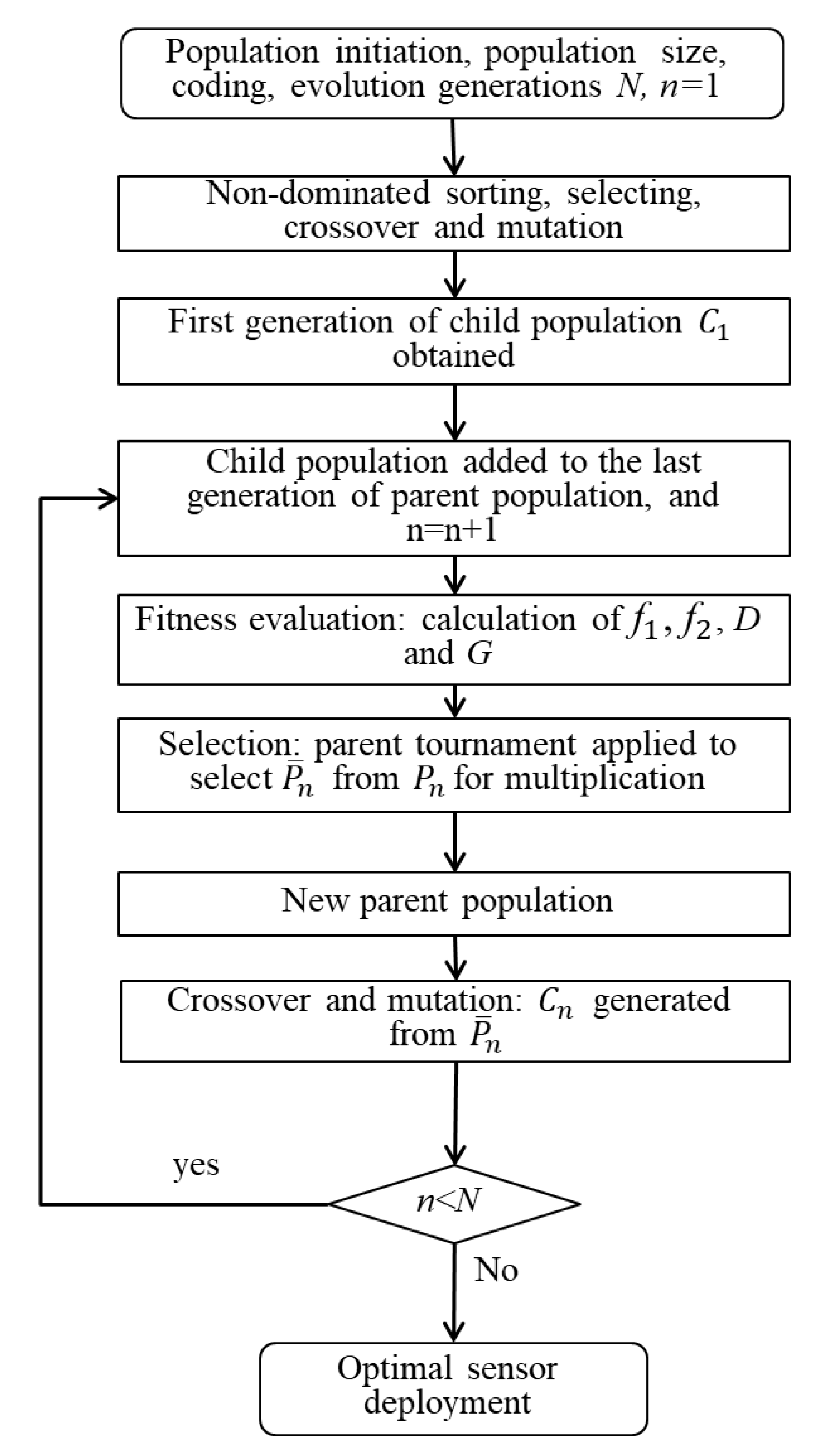
3.3. Solving of Pareto Based Bi-Objective OSP

The evolutionary algorithm is an ideal method for obtaining the Pareto optimal solutions. Srinivas and Deb proposed a non-dominated sorting genetic algorithm and its improved version [36]. Because the NSGA has the defect of high calculation complexity and the obtained satisfactory solutions could be lost during the optimization process, NSGA-II is adopted to solve the problem of Pareto-based bi-objective OSP. Due to the introduction of a fast non-dominated sorting in NSGA-II, the calculation complexity is reduced from $O\left(m{N}^3\right)$ to $O\left(m{N}^2\right)$. In addition, the concept of crowd distance is proposed to maintain the population diversity. The elitist strategy and a crowded-comparison approach are adopted, the population diversity can be maintained, and the loss of the satisfactory solutions can be avoided during the optimization process. The general concept of NSGA-II can be described as follows: The population is firstly initiated, and a non-dominated sorting is carried out of all the individuals in the population. Based on the initial population, the process of selecting, mutation and crossover in genetic algorithms are performed to obtain the first generation. Starting from the second generation, the parent population is merged with the child population to maintain the population diversity. A fast non-dominated sorting is applied, in which an index of the crowding distance is introduced to sort the population and select the parent population combined with the non-dominated grade. The crowding distance can be presented as Equation (12). Finally, a new general child population is generated, and a new round non-dominated sorting and genetic process begins until the prescribed generation number is reached.

$$D\left(i\right)={\displaystyle \sum _{k=1}^m\frac{f_{i+1}\left(k\right)-f_{i-1}\left(k\right)}{f_{\max }\left(k\right)-f_{\min }\left(k\right)}}$$

(12)

where $f_{i+1}\left(k\right)$ and $f_{i-1}\left(k\right)$ are the values of objective function k for (i + 1)th and (i − 1)th individuals in Pareto front; $f_{\max }\left(k\right)$ and $f_{\min }\left(k\right)$ are the maximum and minimum values of objective function k among all the individuals in a certain front. For the individual with the minimum value of the objective function, the crowding distance is defined as infinity, which indicates the priority over other individuals of the same non-dominated grade. The crowding distance considerably increases the calculation efficiency and solution robustness for multi-objective Pareto optimization. Therefore, the NSGA-II is applied in this research to solve the Pareto bi-objective function to obtain the optimal sensor placement positions.

Compared with the traditional genetic algorithm, when NSGA-II is applied to multi-objective OSP, non-dominated sorting, crowding distance estimation and crowding distance comparison operator are used to evaluate individual fitness. Further, a genetic algorithm is adopted to obtain the Pareto front iteratively which meets the requirements of the objective function. The specific implementation steps of the above algorithm are as follows:

(1)

Population initiation

An integer S is defined as the population size. The population ($P_0$) of the sensor placement cases, which contains S individuals, is created. For the subject of sensor placement, the binary encoding is applied to represent the sensor placement positions, of which ‘1’ and ‘0’ represent the positions with and without sensors, respectively.

It is worth noting that when the binary coding method in the genetic algorithm is used for the problems of OSP, the criteria of “Completeness”, “Soundness” and “Non-redundancy” can be met for coding method selection: (i) encoding and decoding are simple to operate. The number of the candidate measuring points is equal to the number of the binary code, in which ‘1’ and ‘0’ represent the positions with and without sensors, respectively, as shown by

Table 1. Example of binary coding of sensor placement positions.

Position Number	Binary Code	With/Without Sensor
1	1	With
2	0	Without
…	…	…
n − 1	0	Without
n	1	With

; (ii) crossover and mutation are easy to realize. For the one-point-crossover, the crossover point is selected at random for one chromosome. The two parent chromosomes exchange the gene segments of each other before or after this crossover point, after which two new individuals are obtained (as shown in Figure 1). Moreover, mutation is also applied to change the binary code of one or more genes for a chromosome (as shown in Figure 2). Such a mutation operation represents that the sensors at those positions are installed or removed, which can avoid the problem of low efficiency and local optimum. (iii) The precision can be satisfied. For the optimization problem of the continuous function, the binary code method has the drawbacks of weak ability of local search and the Hamming Cliff problem. However, for the optimization problems of sensor placement, the discrete solutions constitute the solution set. Consequently, the drawbacks of the binary code method in GA can be avoided for OSP. Therefore, the binary coding method is adopted for NSGA-II in this research.

(2)

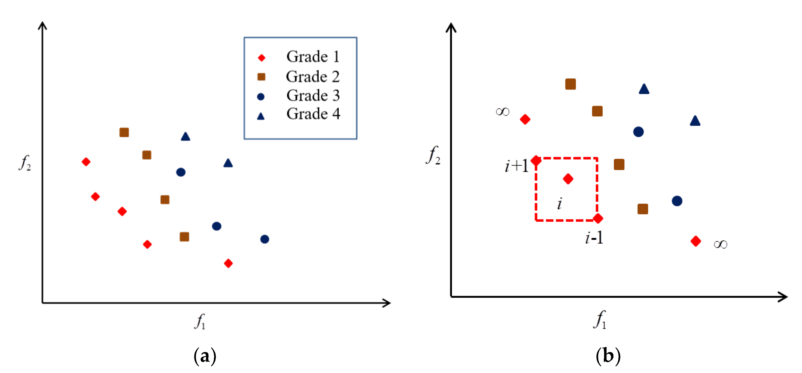
Non-dominated sorting and crowding distance of individuals

The objective functions ($f_1$, $f_2$) are calculated for all the individuals in the initial population, and the non-dominated grades ($G$) are obtained through the non-dominated sorting approach as follows: for each i and j $$$P_0$, if $f_1\left(i\right)<f_1\left(j\right)$ and $f_2\left(i\right)<f_2\left(j\right)$, individual i dominates individual j (i $\succ$ j). If no individual dominates individual i in the population, the non-dominated grade rank 1 and all the individuals with the non-dominated grade 1 constitute the Pareto front 1. The same procedure is carried out for residual individuals iteratively, and the non-dominated grade of all the individuals can be obtained (as shown in Figure 3a). The smaller the number of non-dominated grade, the higher the fitness of individuals in the corresponding front.

For individuals with the same non-dominated grade, the concept of crowding distance is introduced to distinguish their fitness: firstly, individuals with the same dominated grade are sorted according to objective function values in ascending order of magnitude, and the crowding distance of individuals corresponding to the minimum and maximum function values after sorting is defined as infinite. The crowding distance of other individuals is calculated by Equation (12). As shown in Figure 3b, the crowded distance of the $i\text{-th}$ individual ($D\left(i\right)$) in its front is the average side length of the dashed box. When individuals have the same level of dominance, a larger crowding distance represents better fitness.

After obtaining the results of the non-dominated grade and crowding distances, all the individuals can be sorted according to the fitness: if $G\left(i\right)<G\left(j\right)$ or ($G\left(i\right)=G\left(j\right)$ and $D\left(i\right)>D\left(j\right)$), the $i\text{-th}$ individual has a better fitness than the $j\text{-th}$ one.

(3)

Selection

After all the individuals are sorted according to the fitness, the binary tournament selection method is used to select the parents (${\overline{P}}_n$) in the population to produce the offspring. Two individuals were selected from the original population to compare the non-dominated grade and crowding distance, and the individuals with better fitness were selected as the parents for producing offspring. This procedure is repeated until the number of parents reaches half of the original population size.

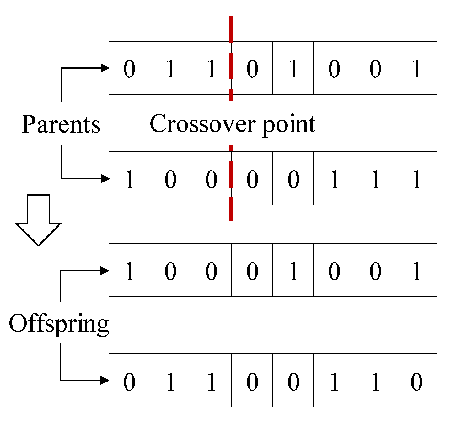
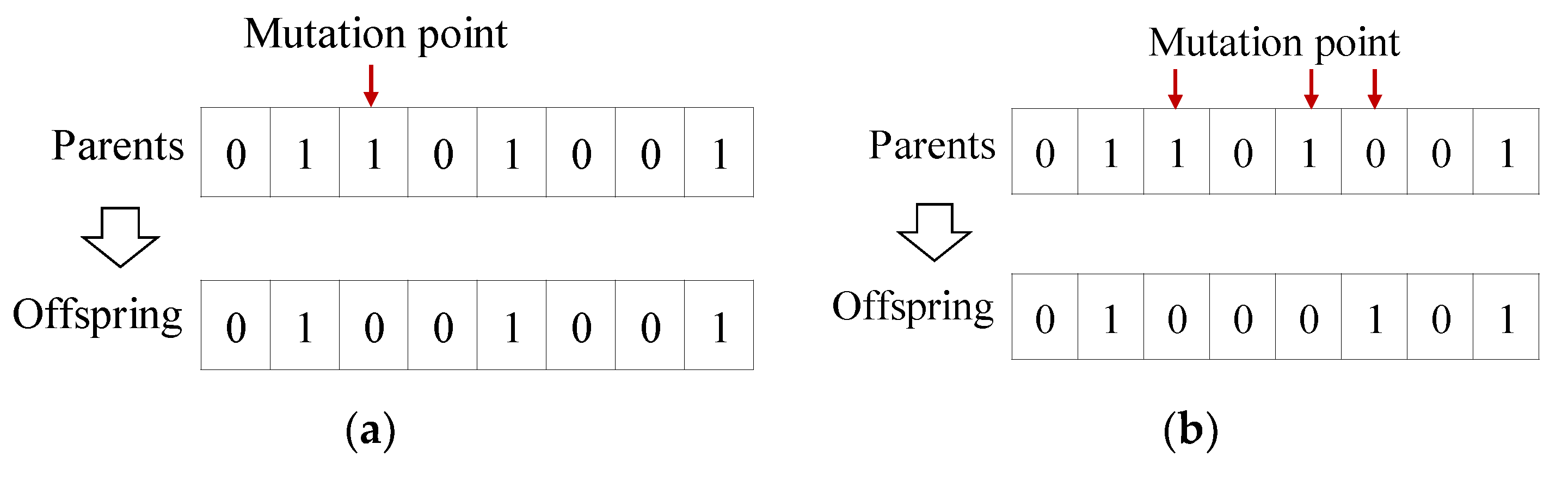
(4)

Crossover and mutation

The offspring ($C_n$) are generated through crossover and mutation. To ensure that the number of sensors remains constant during the genetic process, the mutation method is used to randomly remove or supplement the sensors. Finally, the offspring individuals are added to the initial population, and the first S individuals with best fitness were preserved based on the non-dominated grade and crowd distance, which will produce the new population for the next generation. The iteration process above stops once the target number ($N$) of heredity generations is reached.

The flowchart of the NSGA-II applied in Pareto bi-objective optimization for OSP is shown in Figure 4.

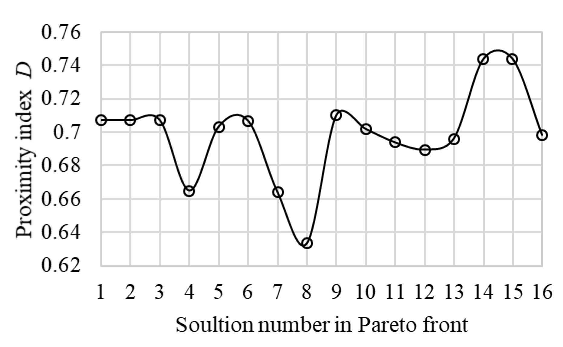
3.4. Comprehensive Evaluation Criteria for Pareto Solutions of OSP

The solution set of a series of OSP schemes can be obtained by the proposed method above. When the engineer has no preference for any single target of senor placement, the obtained solutions are equally optimal in a Pareto sense. However, when some of the solutions in the optimal solution set reach optimum for a single objective function, the solutions degrade to the ones achieved through the traditional single-target sensor placement criteria, which is obviously contrary to the original intention of multi-objective sensor placement. Therefore, a comprehensive evaluation criterion is proposed to determine the final solution from the Pareto optimal solution set for sensor placement when there is no preference for any single criterion.

For the problem of bi-objective OSP, the Pareto OSP solution set $F$ can be expressed as Equations (13) and (14).

$$F=\left[F_1\left(x_1\right),F_2\left(x_2\right),\dots F_k\left(x_k\right)\right]$$

(13)

$$F_k\left(x_k\right)=\left[f_{k1}\left(x_k\right),f_{k2}\left(x_k\right)\right]$$

(14)

where $F_k(•)$ is the $k\text{-th}$ solution of the Pareto optimal solution set; $f_{k1}$, $f_{k2}$ are the two objective function values; $x_k$ is the vector of sensor placement positions corresponding to the $k\text{-th}$ optimal solution. The ideal optimal solution of sensor placement is defined as Equation (15).

$$\begin{gathered} F^{*}=\left[f_1^{*},f_2^{*}\right] \\ \mathrm{s}.\mathrm{t}.f_j^{*}=\underset{1\le i\le k}{\min }\left(f_{ij}\right) \end{gathered}$$

(15)

where $f_{ij}$ is the $j\text{-th}$ objective function value of the $i\text{-th}$ solution in the Pareto solution set. Considering that the different objective functions of OSP are not easy to compare with each other because of their different units and magnitudes, the membership degree $\mu$ is defined to measure the closeness between the values of Pareto solutions and the ideal solutions for each objective function. When $\mu$ approaches 1, the Pareto solution tends to be the ideal solution for OSP. Because the solutions in the Pareto front for OSP can be considered to be randomly distributed, the normal distribution function is selected as the membership function to evaluate the proximity between the Pareto solution and the ideal one. The membership degree vector ${\tilde{F}}_i$ for each Pareto solution is shown as Equations (16) and (17).

$${\tilde{F}}_i=\left[\mu \left(f_{i1}\right),\mu \left(f_{i2}\right)\right]$$

(16)

$$\mu \left(f_{ij}\right)=\exp \left[-{\left(\frac{f_{ij}-f_j^{*}}{\frac{1}{k}{\displaystyle \sum _{i=1}^k\left|f_{ij}-f_j^{*}\right|}}\right)}^2\right]$$

(17)

On the basis of membership vector, a proximity index $D$ is further defined to quantitatively assess the proximity between the Pareto solution and the ideal counterpart, as Equation (18).

$$D_i=\sqrt{\frac{1}{2}{\displaystyle \sum _{j=1}^2{\mu }_{ij}^2}}$$

(18)

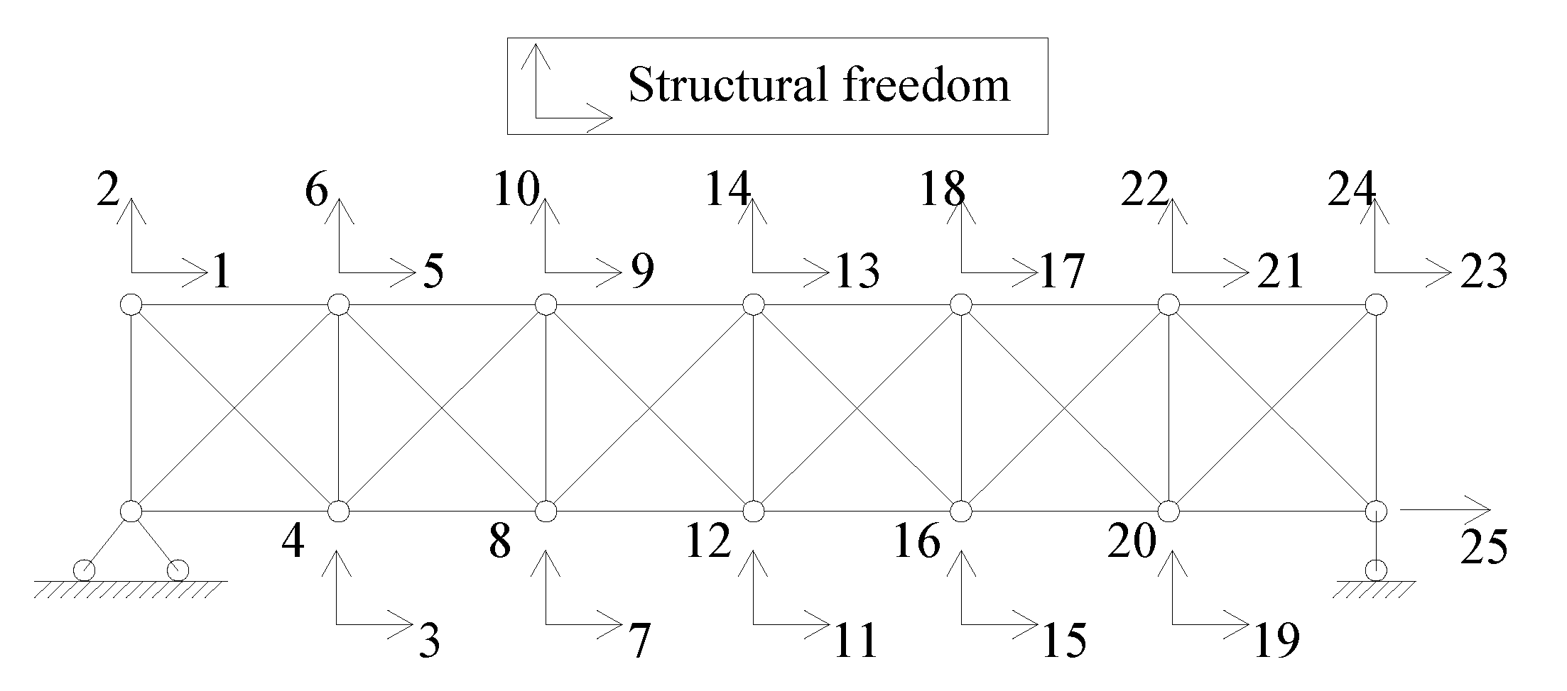
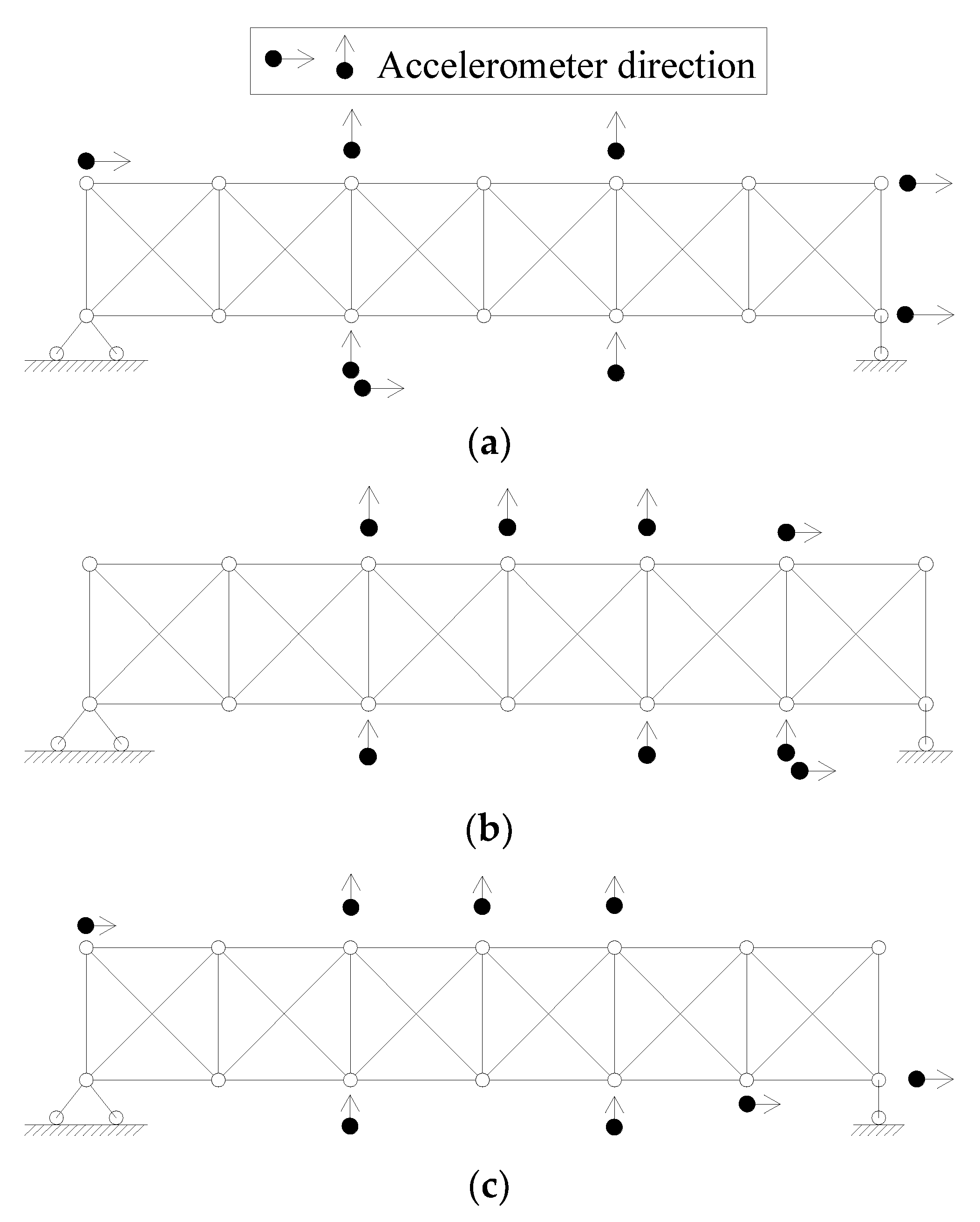
4. Bi-Objective OSP for Plane Truss

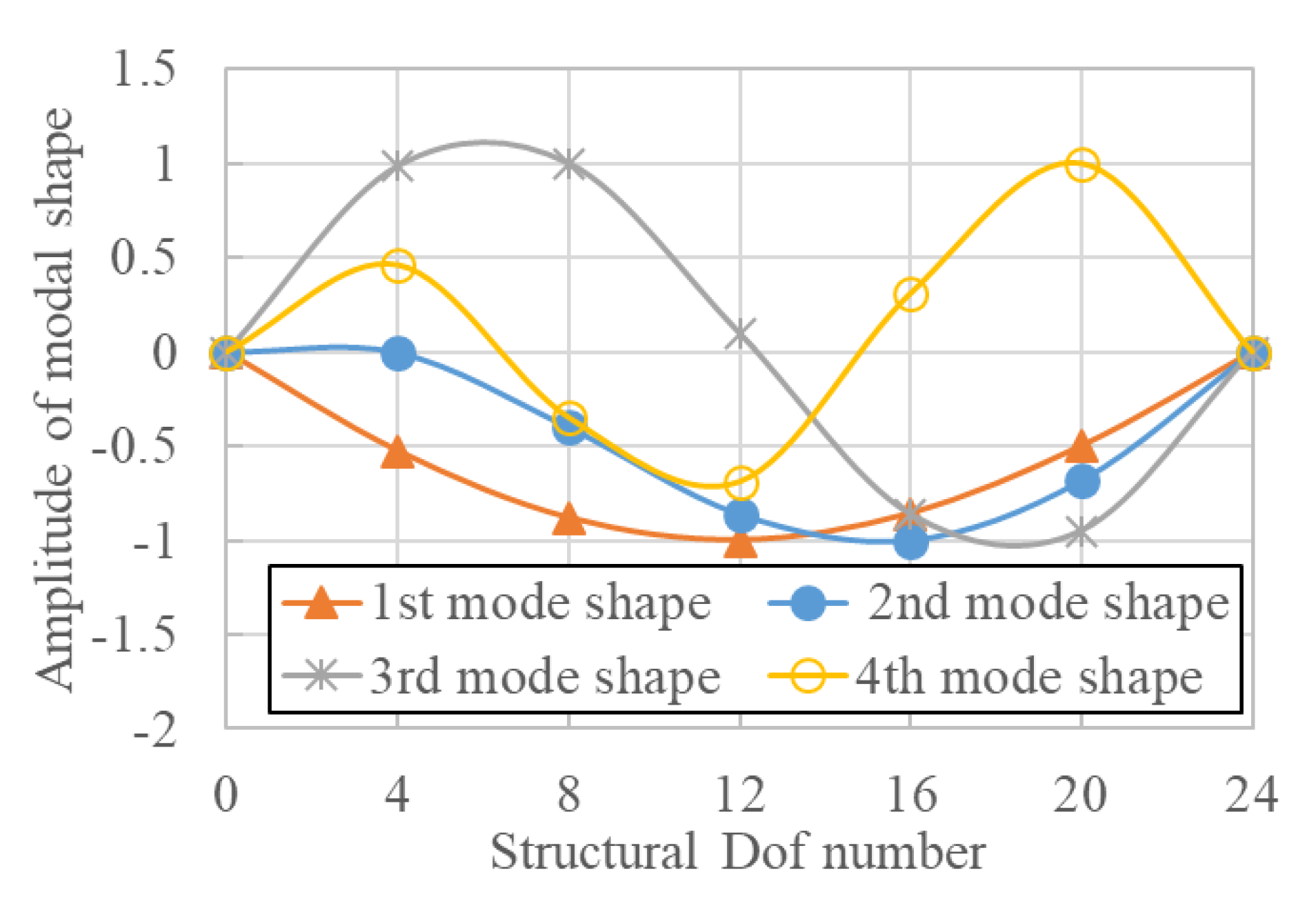
4.1. Properties of Plane Truss

To verify the effectiveness of the bi-objective Pareto optimization for sensor placement, a plane truss is presented as an example to illustrate the application of the proposed method. There are 25 degrees of freedom (Dof) for the truss beam, the elevation of which is presented in Figure 5. The structural modal shapes were obtained through numerical analysis in a previous study. For the modal test, there are eight sensors to be deployed at eight positions selected from 25 candidates to obtain the structural experimental modal. The first four orders of structural modes are considered for the truss beam. Considering that the vertical modes are the main modes of the truss beam, the first four normalized modes are plotted (as shown in Figure 6) using the displacement along the directions of structural Dof number 4, 8, 12, 16 and 20, which are located at the lower side of the truss.

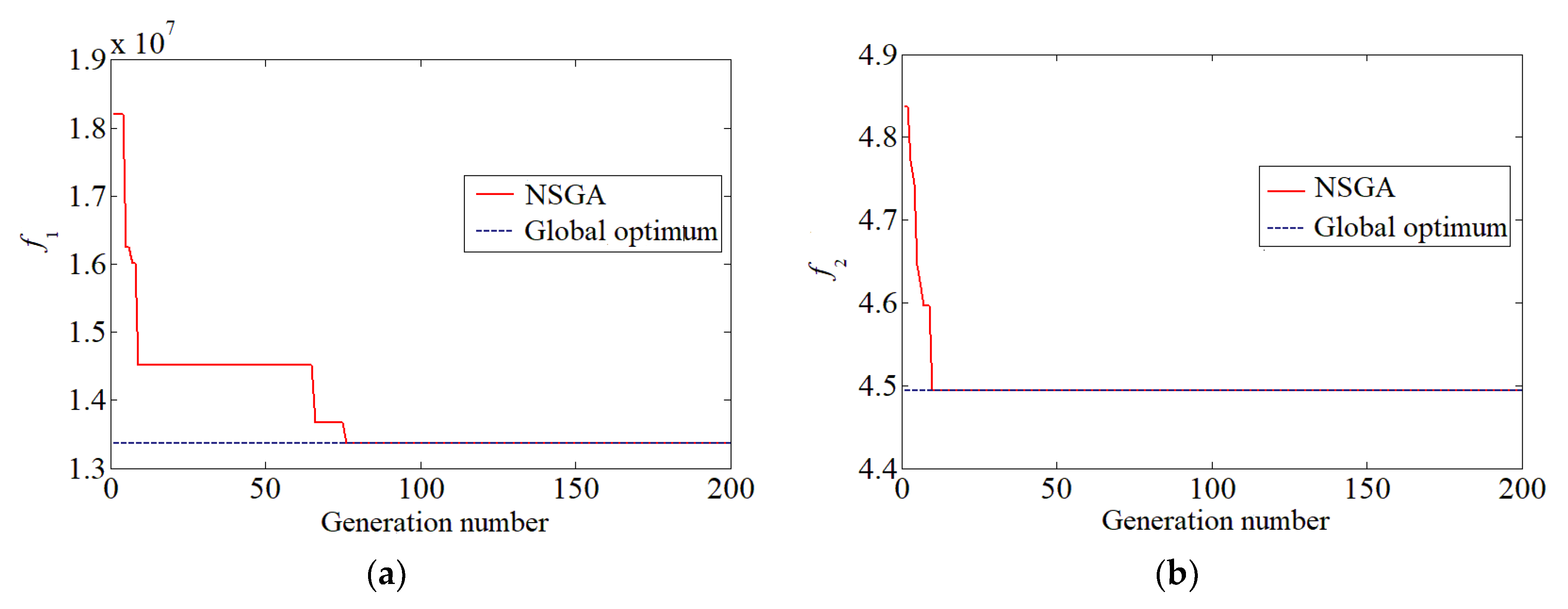
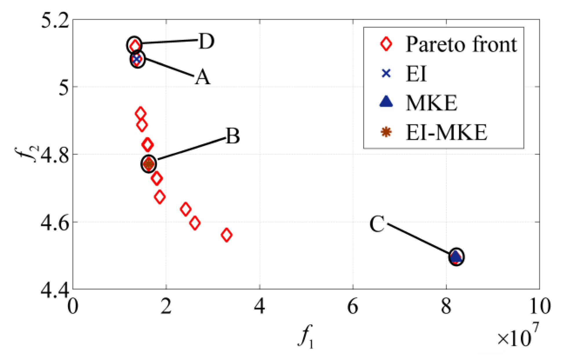
4.2. OSP Proposals

For the sake of simplicity and convenience to illustrate the effectiveness of Pareto based bi-objective optimization, this paper assumes that the main concern of the OSP for the truss beam is to reduce the modal coordinate estimation error and increase the signal-to-noise ratio. In fact, considering any combination of two objective functions does not hinder the effectiveness of the Pareto-based bi-objective optimization method proposed in this paper. Considering EI and MSMKE as criteria of sensor placement, the corresponding bi-objective optimization function is established, and the Pareto optimization analysis is carried out for the OSP position of the plane truss.

To minimize the estimation error of the modal coordination and increase the signal-to-noise ratio of the recorded data, the EI and MSMKE should be considered during the process of OSP. Therefore, Equation (9) should be taken as the objective function for the Pareto bi-objective optimization. The NSGA-II is adopted to solve the bi-objective Pareto optimization considering the functions $f_1$ and $f_2$. During the iterative process, the initial population size of the sensor placement is set to 50. In addition, the crossover and mutation probability are set to 0.9 and 0.1, respectively. The target number of heredity generations is set to 200, which is the threshold used to control the iterative process. The corresponding convergence processes are shown in Figure 7. Compared with the global optimal solutions obtained through the exhaustive method, it can be observed that the two functions $f_1$ and $f_2$ converge to the optimal solution at the generations of 76 and 10, respectively. When the target heredity generation is reached, the iterative process of the NSGA-II terminates, and the Pareto front is output. In addition, the parents are selected through tournament selections to produce the offspring samples. The optimization is implemented according to the iterative process in Figure 4, and the results are plotted in Figure 8. To make comparisons with the results of single-objective functions, the results obtained based on the MSMKE and EI are also presented in Figure 8. Moreover, a traditional bi-objective function considering the EI and MSMKE is illustrated in Equation (19), which transforms the bi-objective optimization into a single-objective optimization. The optimal result of EI- MSMKE is also plotted in Figure 8.

$$\text{EI-MKE}=diag\left(\Phi {\left({\Phi }^T\Phi \right)}^{-1}{\Phi }^T\right)\cdot diag\left(M\Phi {\Phi }^T\right)$$

(19)

As presented in Figure 8, the optimal results for the EI, MSMKE and EI- MSMKE (points ‘A’, ‘B’ and ‘C’ in Figure 8) can all be found in the Pareto front, which means that the bi-objective Pareto optimal results can cover all the results obtained based on the single-objective and traditional bi-objective criteria. The Pareto optimization solved through the NSGA-II can achieve a solution as good as that of the single-objective function of the MSMKE, as shown by point ‘C’ in Figure 8. It is worth noting that the determinant of the Fisher information matrix (point ‘D’ in Figure 8) obtained through the Pareto optimization is even larger than that obtained from the EI, which further verifies the efficiency of the NSGA-II to solve the bi-objective Pareto optimization problem for sensor placement. Moreover, the Pareto front can provide a series of sensor placement schemes that are not worse than the counterpart based on the traditional bi-objective criterion of EI- MSMKE (‘B’ in Figure 8). The sensor placement positions of ‘B’, ‘C’ and ‘D’ in the Pareto front are shown in Figure 9.

4.3. Comprehensive Evaluation of OSP Schemes

The bi-objective optimization results show that the optimal solution set achieved through Pareto optimization method contains 16 equivalent OSP schemes. By adopting the evaluation criteria based on the membership degree index $\mu$ proposed above, the solution from the Pareto optimal solution set, which is closest to the ideal solution, can be determined as the OSP scheme. As shown in Figure 10, solutions No. 14 and 15 have nearly the same value of index $D$ which is the maximum one among all the solutions in Pareto front. It means that the two equivalent OSP solutions can provide alternative schemes when some positions of the structure are inconvenient to install the sensors, and the point ‘B’ in Figure 8 corresponds one of such optimal solutions. Consequently, considering reducing the identification error of modal parameters and increasing vibration signal intensity, the placement positions of the sensors corresponding to point ‘B’ in Figure 8 is optimal for the plane truss.

5. Conclusions

The traditional OSP method is based on single objective criterion, which is generally oriented to meet a single target of sensor placement. When more than one objective is considered to be satisfied, such as improving the identification accuracy of structural modal parameters, the vibration signal strength and the effect of modal reconstruction, the current OSP methods cannot achieve good results. This paper carried out a study on a Pareto-based bi-objective OSP method, and the proposed evaluation criteria of optimal solution can achieve satisfactory results for two objective functions at the same time. The bi-objective OSP method was finally verified through a numerical model of a plane truss. According to the analytical results and discussions, the following conclusions can be drawn:

Pareto optimization can comprehensively consider more than one objective function for OSP, such as the MSMKE, EI and structural modal independence. Compared with the traditional OSP method, the proposed method can make a compromise between the multiple objective functions, and all equally optimal solutions in a Pareto sense can be provided as alternatives for sensor placement, which also covers the sensor placement schemes obtained through the traditional single objective optimization methods.

The NSGA-II is suitable for solving the Pareto optimization problem of OSP for SHM. The bi-objective Pareto optimization of sensor placement can be effectively solved through the NSGA-II and all the equally optimal solutions for the bi-objective OSP can be achieved within a feasible number of generations. The proposed iterative process for the Pareto optimization based on the NSGA-II can be effectively applied to the bi-objective OSP. If more objective functions for OSP are considered, the proposed algorithm can still be effective through multi-objective Pareto optimization.

A comprehensive evaluation method based on membership degree index was proposed for multi-objective OSP, which can quantitatively analyze the proximity between the multiple alternative solutions provided by Pareto optimization and the ideal solutions. By selecting the Pareto optimal solution which has the largest value of proximity index $D$, the corresponding sensor placement scheme can be finally determined among a series of Pareto optimal solutions, and the OSP scheme can achieve good results in both the two objectives.

In this research, the Pareto-based bi-objective optimization functions are established according to three commonly used evaluation criteria for optimal sensor placement, which only involve the optimization of sensor placement positions. In the future, it would be meaningful to carry out research on the multi-objective optimization for both the sensor number and location. In addition, if the evaluation criteria for different types of sensors are introduced to establish objective functions for OSP, the Pareto-based multi-objective optimization method proposed in this paper can be extended for the simultaneous optimization of the different types of sensors on the structure at the same time.

References

- Dharap, P.; Koh, B.-H.; Nagarajaiah, S. Structural Health Monitoring using ARMarkov Observers. J. Intell. Mater. Syst. Struct. 2006, 17, 469–481. [Google Scholar] [CrossRef]
- Sun, L.; Shang, Z.; Xia, Y.; Bhowmick, S.; Nagarajaiah, S. Review of Bridge Structural Health Monitoring Aided by Big Data and Artificial Intelligence: From Condition Assessment to Damage Detection. J. Struct. Eng. 2020, 146, 04020073. [Google Scholar] [CrossRef]
- Yang, D.-H.; Yi, T.-H.; Li, H.-N.; Zhang, Y.-F. Correlation-Based Estimation Method for Cable-Stayed Bridge Girder Deflection Variability under Thermal Action. J. Perform. Constr. Facil. 2018, 32, 04018070. [Google Scholar] [CrossRef]
- Yang, D.-H.; Yi, T.-H.; Li, H.-N.; Zhang, Y.-F. Monitoring and analysis of thermal effect on tower displacement in cable-stayed bridge. Measurement 2018, 115, 249–257. [Google Scholar] [CrossRef]
- Kim, S.; Frangopol, D.M. Multi-objective probabilistic optimum monitoring planning considering fatigue damage detection, maintenance, reliability, service life and cost. Struct. Multidiscip. Optim. 2018, 57, 39–54. [Google Scholar] [CrossRef]
- Leyder, C.; Dertimanis, V.; Frangi, A.; Chatzi, E.; Lombaert, G. Optimal sensor placement methods and metrics–comparison and implementation on a timber frame structure. Struct. Infrastruct. Eng. 2018, 14, 997–1010. [Google Scholar] [CrossRef]
- Ding, Z.; Li, J.; Hao, H.; Lu, Z.-R. Structural damage identification with uncertain modelling error and measurement noise by clustering based tree seeds algorithm. Eng. Struct. 2019, 185, 301–314. [Google Scholar] [CrossRef]
- Nagarajaiah, S.; Yang, Y. Modeling and harnessing sparse and low-rank data structure: A new paradigm for structural dynamics, identification, damage detection, and health monitoring. Struct. Control. Heal. Monit. 2017, 24, e1851. [Google Scholar] [CrossRef]
- Krishnamurthy, P.; Khorrami, F. Optimal Sensor Placement for Monitoring of Spatial Networks. IEEE Trans. Autom. Sci. Eng. 2016, 15, 33–44. [Google Scholar] [CrossRef]
- Loutas, T.; Bourikas, A. Strain sensors optimal placement for vibration-based structural health monitoring. The effect of damage on the initially optimal configuration. J. Sound Vib. 2017, 410, 217–230. [Google Scholar] [CrossRef]
- Pei, X.Y.; Yi, T.H.; Li, H.N. A multi-type sensor placement method for the modal estimation of structure. Smart Struct. Syst. 2018, 21, 407–420. [Google Scholar] [CrossRef]
- Pakzad, S.N.; Fenves, G.L. Statistical Analysis of Vibration Modes of a Suspension Bridge Using Spatially Dense Wireless Sensor Network. J. Struct. Eng. 2009, 135, 863–872. [Google Scholar] [CrossRef] [Green Version]
- Shah, P.C.; Udwadia, F.E. A Methodology for Optimal Sensor Locations for Identification of Dynamic Systems. J. Appl. Mech. 1978, 45, 188–196. [Google Scholar] [CrossRef]
- Limongelli, M.P. Optimal location of sensors for reconstruction of seismic responses through spline function interpolation. Earthq. Eng. Struct. Dyn. 2003, 32, 1055–1074. [Google Scholar] [CrossRef]
- Stephan, C. Sensor placement for modal identification. Mech. Syst. Signal Process. 2012, 27, 461–470. [Google Scholar] [CrossRef]
- Kammer, D.C. Sensor placement for on-orbit modal identification and correlation of large space structures. J. Guid. Control Dyn. 1991, 14, 251–259. [Google Scholar] [CrossRef]
- Papadopoulos, M.; Garcia, E. Sensor Placement Methodologies for Dynamic Testing. AIAA J. 1998, 36, 256–263. [Google Scholar] [CrossRef]
- Carne, T.G.; Dohrmann, C.R.; Soc, E.M. A modal test design strategy for model correlation. In Proceedings of the 13th International Modal Analysis Conference, Albuquerque, NM, USA, 13–16 February 1995; Volume 2460, pp. 927–933. [Google Scholar]
- Li, D.; Li, H.; Fritzen, C. The connection between effective independence and modal kinetic energy methods for sensor placement. J. Sound Vib. 2007, 305, 945–955. [Google Scholar] [CrossRef]
- Yi, T.-H.; Li, H.-N.; Song, G.; Zhang, X.-D. Optimal sensor placement for health monitoring of high-rise structure using adaptive monkey algorithm. Struct. Control. Heal. Monit. 2015, 22, 667–681. [Google Scholar] [CrossRef]
- Yi, T.-H.; Li, H.-N.; Zhang, X.-D. A modified monkey algorithm for optimal sensor placement in structural health monitoring. Smart Mater. Struct. 2012, 21, 21. [Google Scholar] [CrossRef]
- Thiene, M.; Khodaei, Z.S.; Aliabadi, M.H. Optimal sensor placement for maximum area coverage (MAC) for damage localization in composite structures. Smart Mater. Struct. 2016, 25, 095037. [Google Scholar] [CrossRef]
- Salmanpour, M.S.; Sharif Khodaei, Z.; Aliabadi, M.H. Transducer placement optimisation scheme for a delay and sum damage detection algorithm. Struct. Control. Health Monit. 2017, 24, e1898. [Google Scholar] [CrossRef] [Green Version]
- Casciati, S.; Faravelli, L.; Chen, Z. Energy harvesting and power management of wireless sensors for structural control applications in civil engineering. Smart Struct. Syst. 2012, 10, 299–312. [Google Scholar] [CrossRef]
- Sankary, N.; Ostfeld, A. Multiobjective Optimization of Inline Mobile and Fixed Wireless Sensor Networks under Conditions of Demand Uncertainty. J. Water Resour. Plan. Manag. 2018, 144, 04018043. [Google Scholar] [CrossRef]
- Soman, R.N.; Onoufriou, T.; Kyriakides, M.A.; Votsis, R.A.; Chrysostomou, C.Z. Multi-type, multi-sensor placement opti-mization for structural health monitoring of long span bridges. Smart Struct. Syst. 2014, 14, 55–70. [Google Scholar] [CrossRef]
- Azarbayejani, M.; El-Osery, A.; Taha, M.M.R. Entropy-based optimal sensor networks for structural health monitoring of a cable-stayed bridge. Smart Struct. Syst. 2009, 5, 369–379. [Google Scholar] [CrossRef]
- Cha, Y.; Raich, A.; Barroso, L.; Agrawal, A. Optimal placement of active control devices and sensors in frame structures using multi-objective genetic algorithms. Struct. Control. Heal. Monit. 2011, 20, 16–44. [Google Scholar] [CrossRef]
- Ostachowicz, W.; Soman, R.; Malinowski, P. Optimization of sensor placement for structural health monitoring: A review. Struct. Health Monit. 2019, 18, 963–988. [Google Scholar] [CrossRef]
- Ahlawat, A.S.; Ramaswamy, A. Multiobjective Optimal Structural Vibration Control Using Fuzzy Logic Control System. J. Struct. Eng. 2001, 127, 1330–1337. [Google Scholar] [CrossRef]
- Marsh, P.S.; Frangopol, D.M. Lifetime Multiobjective Optimization of Cost and Spacing of Corrosion Rate Sensors Embedded in a Deteriorating Reinforced Concrete Bridge Deck. J. Struct. Eng. 2007, 133, 777–787. [Google Scholar] [CrossRef]
- Huang, Y.; Ludwig, S.A.; Deng, F. Sensor optimization using a genetic algorithm for structural health monitoring in harsh environments. J. Civ. Struct. Heal. Monit. 2016, 6, 509–519. [Google Scholar] [CrossRef]
- Tan, P.; Dyke, S.J.; Richardson, A.; Abdullah, M. Integrated Device Placement and Control Design in Civil Structures Using Genetic Algorithms. J. Struct. Eng. 2005, 131, 1489–1496. [Google Scholar] [CrossRef]
- Beygzadeh, S.; Salajegheh, E.; Torkzadeh, P.; Salajegheh, J.; Naseralavi, S.S. An Improved Genetic Algorithm for Optimal Sensor Placement in Space Structures Damage Detection. Int. J. Space Struct. 2014, 29, 121–136. [Google Scholar] [CrossRef]
- Rao, A.R.M.; Anandakumar, G. Optimal placement of sensors for structural system identification and health monitoring using a hybrid swarm intelligence technique. Smart Mater. Struct. 2007, 16, 2658–2672. [Google Scholar] [CrossRef]
- Srinivas, N.; Deb, K. Multiobjective optimization using non-dominated sorting in genetic algorithms. Evol. Comput. 1994, 2, 221–248. [Google Scholar] [CrossRef]