Cost Modeling from the Contractor Perspective: Application to Residential and Office Buildings

Abstract

For the majority of the contractual arrangements used in construction projects, the owner is not responsible for the cost deviations due to the variability of labor productivity or material price, amongst many other aspects. Consequently, the cost performance of a project may be entirely distinct for the owner and the contractor. Since the majority of quantitative research on cost estimation and deviation found in the literature adopts the owners’ perspective, this research provides a contribution towards modeling costs and cost deviation from a contractor’s perspective. From an initial sample of 13 residential buildings and 10 office building projects, it was possible to develop models for cost estimation at the early stage of development, including both endogenous and exogenous variables. Although the sample is relatively small, the authors were able to fully analyze all the cost data, using no secondary sources of data (which is very frequent in cost modeling studies). The statistically significant variables in the cost estimation models were the areas above and below ground and the years following the 2008 financial crisis, including the international bailout (2011–2014) period. For estimating the unit cost, a nonlinear model was obtained with the number of underground and total floor, the floor ratio, and the years following the 2008 financial crisis, including the international bailout (2011–2014) period as predictors. For the office buildings, a statistically significant correlation was also found between the cost deviation and number of underground floors.

1. Introduction

The complexity of construction projects is increasing, both on their “hard” (or tangible) and “soft” (or intangible) dimensions. From new materials to new construction technologies, a multitude of technical solutions have emerged over the last few decades, widening the range of alternative options available for the “hard” dimension of construction projects. Concurrently, the range of aspects to manage in construction project has also increased. The “soft” dimension of construction projects includes the need for satisfying an increasingly broader and stringent social (e.g., health and safety), environmental (e.g., construction and demolition waste management), and economic (e.g., use of life-cycle cost as awarding criteria on public projects in the European Union) requirements. Consequently, construction managers are now facing additional challenges in their projects. To aid them in their tasks, several standards and regulations have been published (e.g., ISO 21,500 family of standards) and new tools are becoming available (e.g., BIM—Building Information Modeling). These provide holistic and consistent guidelines and technological support to tackle the complexity of managing construction projects within this new context.

Despite all these evolutions, the financial control of construction projects is still a dominant dimension in a project’s governance. In this regard, cost estimation in the early stages dictates the investment decisions, although, at the early stages, there is a significant risk surrounding the estimation, given the technical uncertainty. Therefore, more accurate cost forecasting in the early stages of the project’s development and better quantification/understanding of cost deviations are amongst the key concerns of any construction project manager [1].

Within this research, the contractor perspective is adopted by analyzing the financial performance of 23 building projects of a large industrial group in Portugal (13 residential buildings and 10 office building projects). Among the companies in the group, there is real estate and a contractor that develop, amongst other types of projects, residential and office buildings in collaboration. Although the dataset is relatively small, it is homogenous, in the sense that the contractor was the same company, and the cost analysis used no secondary data. The real estate assumes all the licensing, design, marketing, and commercialization and the contractor executes the projects. The contractor also develops projects for external clients, both private and public, of various types (e.g., commercial, healthcare, and educational buildings; water, transportation, and energy infrastructures).

The paper is organized as follows. After the introduction, Section 2 presents the literature review, Section 3 explains the data used and the methods, Section 4 presents the results, and, finally, Section 5 provides the main conclusions.

2. Literature Review

Historically, there have been several tools for cost estimating at early stages of a project’s development. The simplest models are based on parametric estimation of costs, built upon expert judgments (see for instance, [2]). The traditional multiple regression analysis (RA) has been the tool most used by researchers (e.g., [3,4]). Artificial neural networks (ANN) have gained some expression for data modeling in various engineering problems, including cost estimation (e.g., [1,5,6]), and case-based reasoning (CBR) is also being used in various tasks related to construction management (e.g., resource estimation—[7]; duration estimation—[8]). A review on CBR use for construction management can be found in [9] and its use for cost estimation can be found in [10,11,12]. A comparison between the three methods was done by [13], with the new tools achieving better results than regression models. More recently, [14] developed cost estimation models using support vector machines, along with ANN combined with an unsupervised deep Boltzmann machine, and included exogenous variables (e.g., consumer price index, interest rate for loan, population of the city) in combination with endogenous variables (e.g., total area). Some authors have also developed models to estimate the cost of portions of the projects (e.g., structure—[15,16]).

Table 1. Early-stage cost estimation models for buildings.

Reference	[21]	[22]	[23]	[24]	[25]	[26]	[27]	[28]	[29]	[30]	[31]	[32]	[33]
Method
Regression Analysis	X		X	X	X	X		X	X	X	X
Artificial Neural Network		X	X		X								X
Case-Based Reasoning												X
Other							X
Variables
Project related
Building type		X				X		X		X
Area	X	X	X					X		X	X	X	X
Number of stories		X	X							X		X	X
Number of households												X
Height			X	X				X	X				X
Duration		X	X		X				X		X
Location			X								X
Above ground external envelope characteristics	X		X								X
Underground external envelope characteristics	X		X
Number of lifts			X								X	X
Number of piloti floors												X
Structural characteristics			X
Other			X		X		X		X		X	X
Management related
Type of contract			X			X	X
Procurement strategy			X		X	X	X
Other			X		X
Other
Type of client						X	X
Construction year	X									X
Designer characteristics							X
Contractor characteristics								X
Site characteristics			X
Sample
Size	15	30	288	36	50	93	-	30	290	42,340 18,469	75	91	232
Type	R	S	R				-	O		R O	R	R

R—Residential buildings. O—Office buildings. S—School buildings.

summarizes the main research on the topic, along with the methods and explanatory variables used in each study. It should be noted that some models were developed to estimate the total cost (when the area is included in the model) whereas others were developed to estimate the unit cost (when the area is not included in the model). Some variables listed in Table 1 should be interpreted as a category of variables rather than a single variable, in some cases simply because they are measured differently depending on the author. For instance, the construction area may be gross, usable, or other; the number of stories may also be total, above ground, and underground; or the height may be of the building or of the floor. Others are naturally a category of variables, such as the structural characteristics that may include the type of structure or foundation (e.g., [17]). A few are even impossible to quantify adequately at the early stages of the project development, namely the duration. In fact, it is far more common to use cost as an independent variable to estimate the construction duration (e.g., see [18,19,20]) for examples of time-relationships), because a cost estimate tends to be done by the designer before the contractor develops the construction schedule.

There are also authors attempting to use BIM for conceptual cost estimation (e.g., [34]). However, this approach requires a quantities takeoff, which implies a degree of project development that is incompatible with the early stages of development in this research (definition of general characteristics of the project, such as area and number of floors, and a preliminary sketch). In fact, even some models reported in the literature review presented herein use variables that may be unavailable at this stage of the project development (e.g., proportion of walls and windows in the external envelope). There is a clear trade-off between model adjustment, i.e., estimation accuracy and the availability of information in the early stages of the project. The review presented focused on cost estimation for building projects and is not intended to be exhaustive, but rather illustrates that different tools, sample sizes, and variables have been used. There is also an extensive literature on other types of projects (e.g., transportation infrastructure projects—[35,36,37,38,39]).

The topic of cost deviations is closely related to cost estimation, since a more accurate cost estimation should reduce cost deviations. There is an extensive literature on the magnitude (e.g., [40,41,42,43,44,45,46]) and causes (e.g., [47,48,49,50,51]) of cost deviations. The former tends to be quantitative, based on the analysis of the performance of past project, while the latter is mostly qualitative, resorting to questionnaires or interviews with experts.

The research relating the magnitude with the causes of cost deviation is less extensive and the causes are limited to macro variables of the projects, such as: (i) The size of the project ([52,53]); (ii) the nature of ownership/promotor (public or private—e.g., [41,54]); (iii) the type of intervention (new build or refurbishment/rehabilitation—[40]); (iv) the type of project (residential, infrastructure, commercial, and other—e.g., [55]); (v) the procurement model (design-bid-build, design and build, project management—e.g., [52,56]); or (vi) the tender method (open, selection, negotiated tendering—e.g., [57]).

Most research on cost modeling in general (cost estimation and cost deviations) tends to focus on variables endogenous to the projects. Table 1 provides a clear illustration of this claim, with the variables used by the various authors being exclusively related to the project or its management. There is a smaller body of literature on the influence of exogenous variables on the financial performance of construction projects. For instance, Refs. [58,59,60] demonstrated the relation between political and economic cycles and the cost deviation in public projects.

The quantitative research available in the literature, both in terms of cost estimation and quantitative analysis of cost variations, tends to reflect the construction projects’ financial performance from the owners’ perspective. The records used by most of the authors were obtained from the owners (or from the contractors) and represent the payments made to the contractors and not the expenses of the contractors. However, the amounts payed by the owners do not match perfectly the amounts spent by the contractors to execute the projects after deducting the profit margin. Regarding the cost estimation, the owners’ perspective is affected by the commercial strategy adopted by the contractors in each moment, frequently represented by the margin defined in their bids. In highly competitive contexts, the margins tend to decrease, whereas in low competitive contexts the margins tend to increase. Concerning cost deviations, the variability of materials prices, labor productivity, or site overheads, amongst other potential causes of cost deviation (e.g., accidents, equipment breakdown, or failure) are not measured when analyzing historical construction cost data from the owner’s perspective. From the owner’s perspective, change orders and errors/omissions (if the design is provided by the owner) are the most relevant causes of cost deviations.

The literature has provided recently an active discussion whether cost deviations are motivated by more technical aspects (e.g., cost escalation, scope changes, unforeseen events/conditions) of the projects ([43,44]) or by estimator bias ([61,62]). However, this discussion is outside of the scope of the present research. This discussion focuses on the cost deviations between the first estimate and final cost, and in the context of major infrastructure projects more applicable to public projects. This includes references to the benefits of the projects for society. Herein, the scope is restricted to private projects and cost deviations between the detailed design and final cost. Furthermore, the cost-benefit ratio is simply the cost of the project versus the income generated by its commercialization. Thus, fundamentally the technical aspects will drive the cost deviations and the potential estimator bias will be more on the expected market valuation of the project.

3. Data and Methods

As referred above, the data used was obtained from a large industrial group in Portugal that include a real estate and a contractor in their portfolio of companies. All projects were developed in collaboration between these two companies of the group and, despite the formal split between them, they end up working as a single entity with complementary expertise.

The 23 building projects were developed mostly in Portugal, with only 2 being abroad (Angola and Mozambique). The projects in Portugal are concentrated in the Lisbon and Porto metropolitan areas (the two major cities in Portugal) and can be classified as premium. The projects in Africa are located in the capital cities of the respective countries (Luanda, in Angola, and Maputo, in Mozambique). Naturally, there are differences between the Portuguese and African contexts at various levels, but the projects are all new developments in consolidated urban areas. Focusing on the Portuguese projects, infrastructures (e.g., roads, water, electricity, communications) and support facilities (e.g., subcontractors, suppliers) are good and can be regarded equivalent in both Lisbon and Porto regions. Furthermore, since the projects are all from the same group, the management approach and skills can be considered identical and, in many cases, the designers were also the same. The projects in Portugal also resorted to the same subcontractor and suppliers in many instances.

Information on the projects includes the: (i) Proportion of the cost by major category of works (structure, architecture, technical installations, and site overheads); (ii) estimated cost; (iii) profit margin; (iv) estimated price; (v) final price; (vi) total area, above ground, and underground gross-built area; and (vii) total floors, above ground, and underground number of floors. There is also information on the start year and duration of the projects. Both the cost and prices of the projects were update to 2019 values using the formulas for price adjustment applicable to public residential and office buildings in Portugal. In Portugal, the reimbursements to contractors in public construction projects are corrected to account for inflation. Since this is mandatory, there are formulas defined by law for estimating the increase (or decrease) in the payments to the contractor for 23 different types of projects (Law-Decree n° 6/2004). These formulas represent the average weight of labor, materials (a selection from 51 different materials), and equipment on the total price of the projects. The price indexes of the labor, materials, and equipment are published monthly by the government based on the official inflation data. The estimated and final unit prices and the cost deviations were calculated from the available data. It was not possible to retrieve all the fields for all the projects, particularly the final price that was available for only 16 projects.

In addition to the endogenous variables, the influence of the 2008 financial crisis and subsequent international bailout that Portugal had between 2011 and 2014 was also included. This exogenous variable was modeled with a categorical predictor assuming the value of 1 between 2008 and 2014 and 0 in the remaining years. A lag of 1 year was also considered at the start and end of the crisis to evaluate if there was a delay between these events and the impact on the cost of the projects.

Due to confidentiality issues regarding some of the data (revealing the cost without the profit margin of the contractor for an external client), indexes were computed dividing the value of each project by the average of all the projects in the sample. This was done particularly for the projects profit margin, total and unit cost, as well as total, unit initial, and final prices. Area and floor ratios were also computed dividing the values above ground by the values underground since there is typically a relation both due to parking requirements.

A statistical approach was used to analyze the data, comprising of two steps: (i) A preliminary data analysis and (ii) data modeling. The preliminary data analysis included calculation of descriptive statistics, assumptions testing, and unidimensional statistical analysis. The normality and homogeneity of variance were tested using the Shapiro–Wilk and Levene’s tests, respectively, and the unidimensional analysis was done using either parametric or non-parametric distribution comparison (t-test/ANOVA or Mann–Whitney/Kruskal–Wallis), for categorical variables, and correlation (Pearson or Spearman), for continuous variables. The data modeling was based on the traditional least squares multiple linear regression. Non-linear regression was also used, when necessary, but given the sample size, the use of artificial intelligence tools (e.g., artificial neural networks, support vector machines, random forests) was not considered. Given the small sample size, bootstrapping (1000 simulations with simple sampling and 95% confidence interval based on percentile) was used to strengthen the confidence in the results.

The restriction of the context (projects from a single company), scope (all buildings are classified as premium in terms of quality), and location (the spatial variability of the locations is small) limits the generalization of the results. However, it excludes these variables from the cost estimation and deviations of the projects and enables the possibility of capturing the cost estimation and deviations drivers that are specific to the projects. This is an important difference from most past research effort, which in most cases use data samples with projects that may be very different, developed by distinct contractors, designed by different teams, and, in some cases, promoted by various owners in many locations. This broader scope allows capturing an overall average cost performance of the projects, but it is impossible to assess if it was due to the contractor competence, design quality, owner experience, nature of the project, local factors, or other aspects that are controlled for in the analysis. Consequently, using large mixed samples of data may fail in terms of applicability to a specific project.

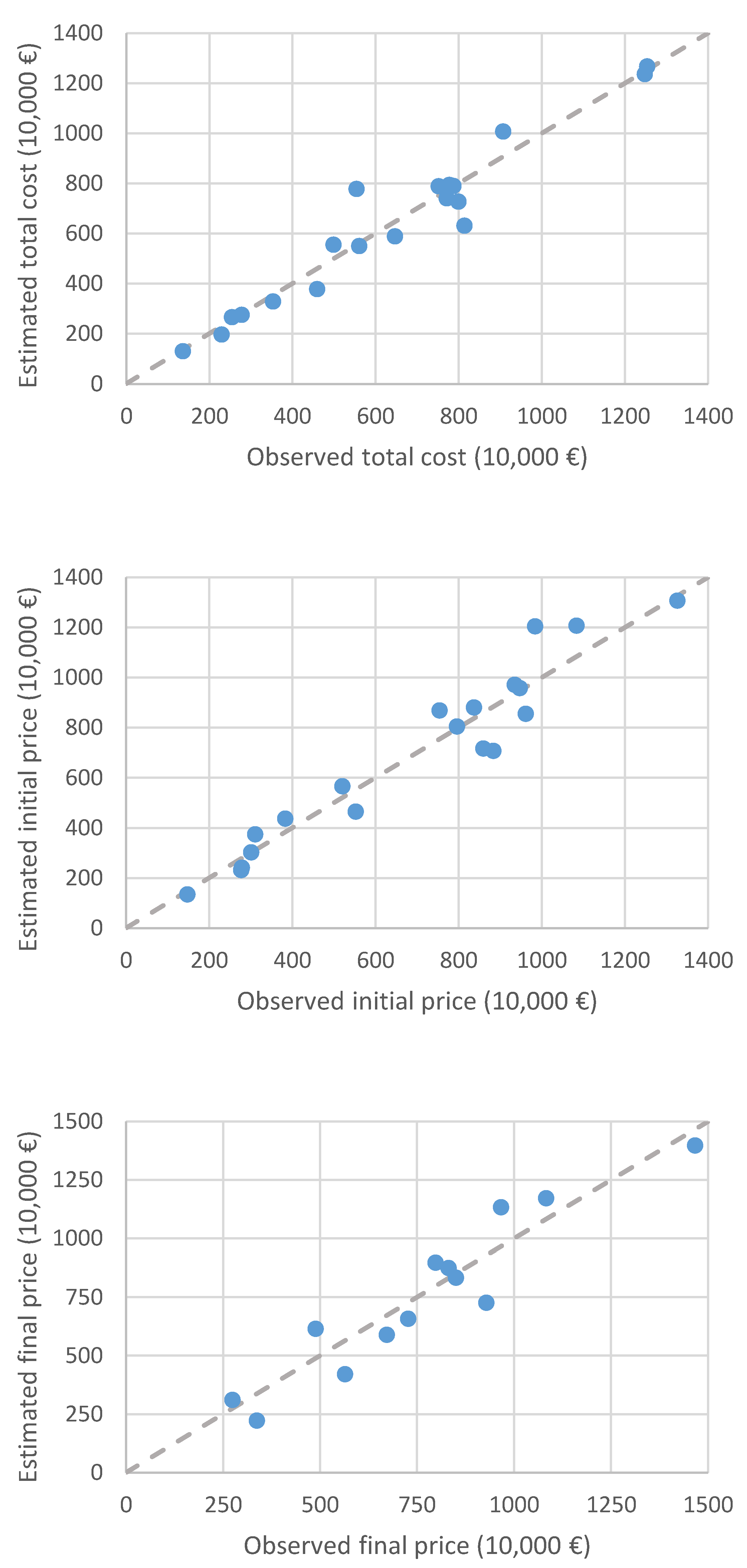
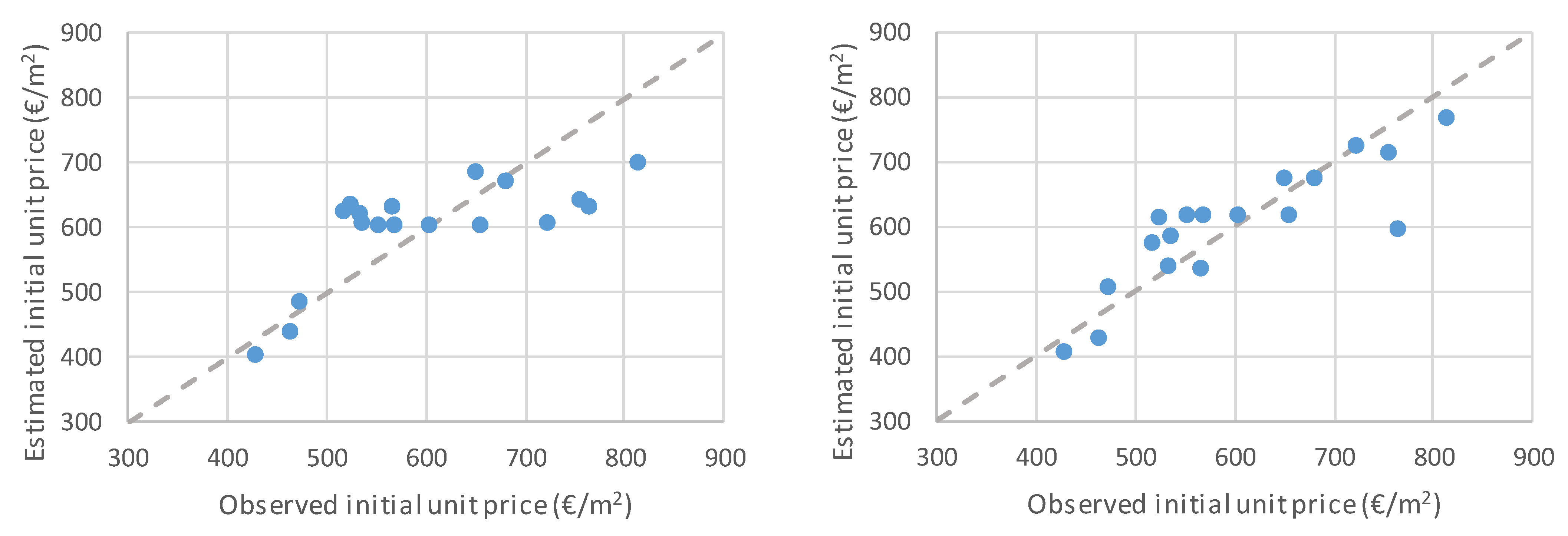
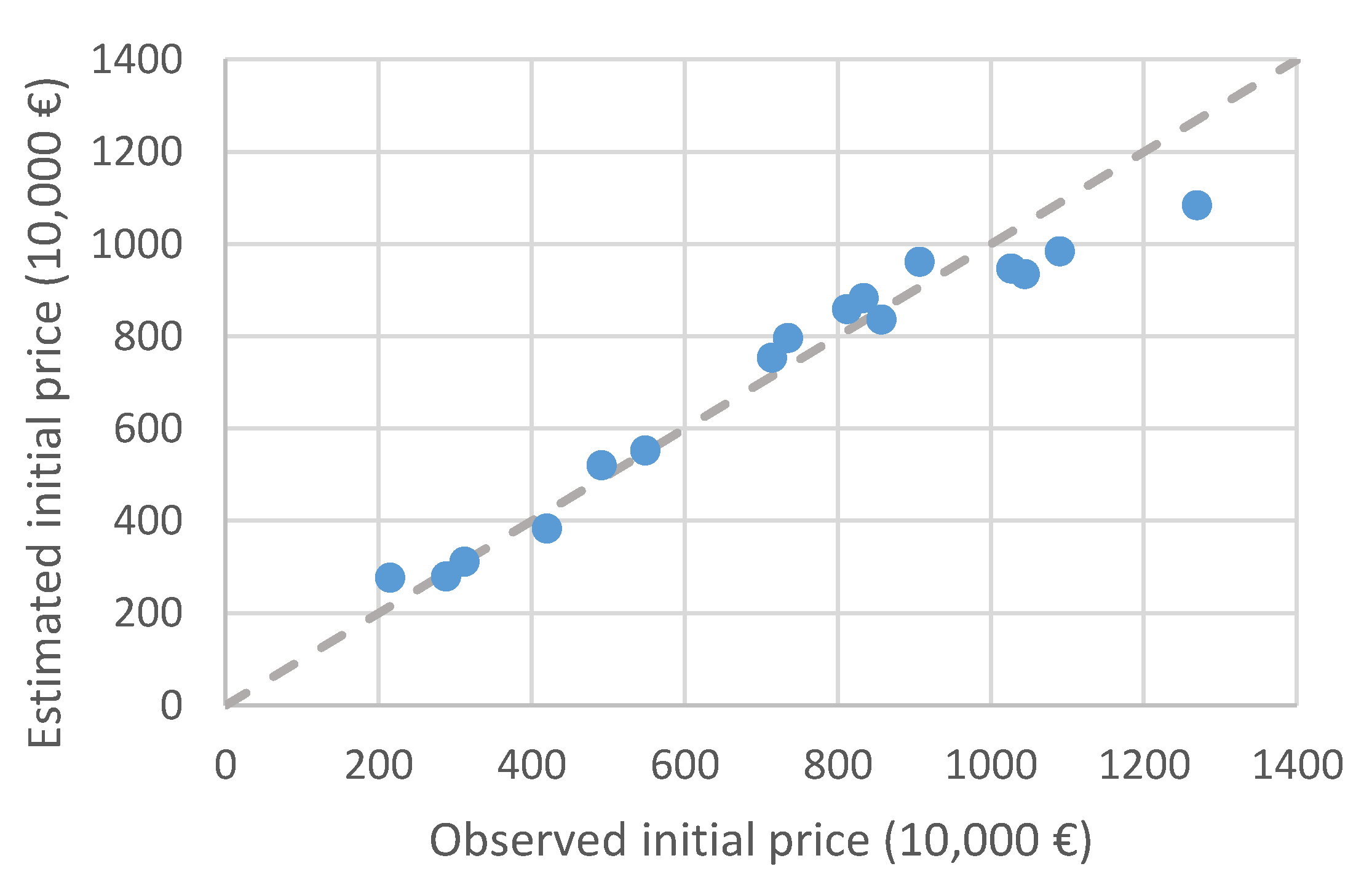
4. Results and Discussion

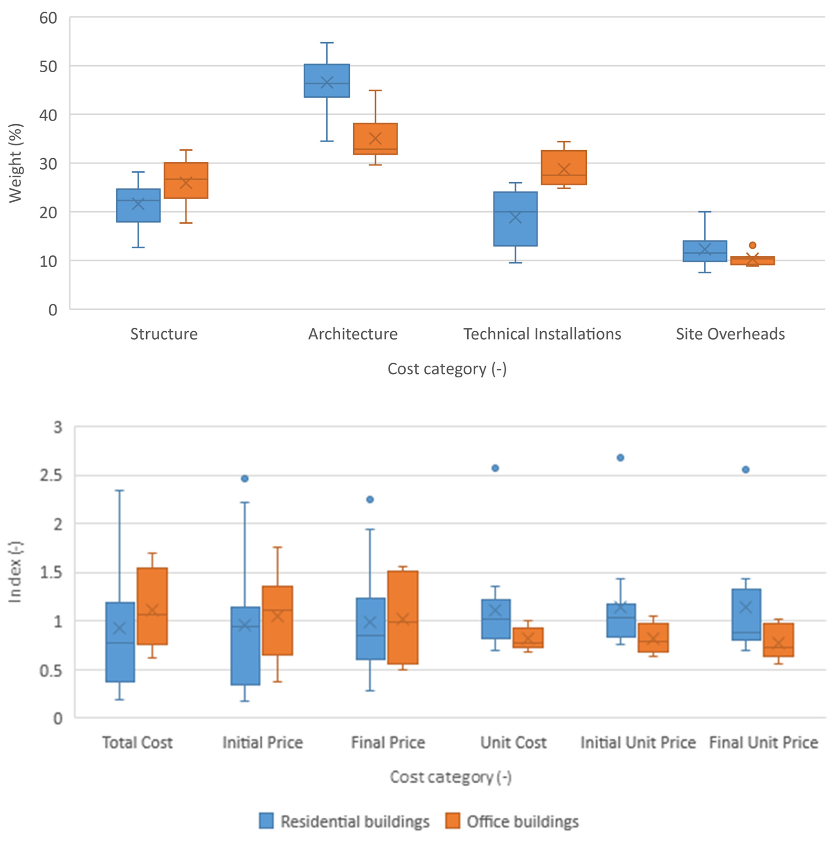
4.1. Preliminary Data Analysis

As defined in Section 3, a preliminary data analysis was carried out comprising an overall statistical characterization of the projects in the sample, followed by the statistical analysis of the distribution of costs by major categories of works (structural works, architectural works, technical installation works, and site overheads). The latter provides information, not only on the typical distribution of costs by category, but assesses if there statistically significant differences depending on the type of building.

The projects totalize a cost of over 155 million euros, with the residential buildings contributing 57% and the office buildings accounting for 43%. The initial price (cost plus typical margin used by the contractor for external clients) of each individual project ranged from 1.5 to 20 million euros. The average initial unit price is 560 €/m² for office buildings, and 785 €/m² for residential buildings. This difference is, however, strongly influenced by the two residential buildings outside Portugal (one in Angola and another in Mozambique) that had an average initial unit price of 1408 €/m².

Table 2. Descriptive statistics of some of the main variables in the dataset.

Variable		Sample	Range	Minimum	Maximum	Sum	Mean	Std. Dev.	Skewness	Kurtosis
Floors (-)	Underground	19	4	1	5	64	3.37	1.065	−0.849	1.152
	Above Ground	21	20	3	23	153	7.29	4.880	2.162	4.987
	Total	19	16	5	21	189	9.95	3.837	1.424	2.528
	Ratio	19	6.25	0.75	7.00	42.48	2.24	1.531	1.944	4.278
Area (m2)	Underground	22	16,893.00	420.00	17,313.00	131,353.75	5970.63	4184.18	0.905	0.926
	Above Ground	22	10,342.00	1557.00	11,899.00	142,095.44	6458.88	2983.97	0.221	−0.740
	Total	23	26,136.00	1977.00	28,113.00	294,621.19	12,809.62	6671.70	0.287	−0.311
	Ratio	22	3.08	0.62	3.71	33.14	1.51	0.833	0.935	0.661
Cost Category Weight (%)	Structure	23	20.00	12.70	32.70	540.30	23.49	5.019	−0.237	−0.398
	Architecture	23	25.10	29.60	54.70	955.70	41.55	7.751	−0.128	−1.420
	Technical Installations	23	24.90	9.50	34.40	532.60	23.16	6.822	−0.425	−0.449
	Site Overheads	23	12.50	7.50	20.00	263.40	11.45	2.988	1.598	2.854
Total Cost Index (-)		21	21	2.11	0.19	2.29	21.00	0.126	0.333	0.501
Margin Index (-)		21	21	1.96	0.36	2.32	21.00	0.134	0.375	0.501
Price (-)	Initial	22	19,367,364.57	1,477,203.03	20,844,567.61	185,850,166.26	8,447,734.83	5,107,220.52	0.873	0.610
	Final	16	19,159,444.23	2,746,435.50	21,905,879.73	155,809,085.39	9,738,067.84	5,404,338.41	0.970	0.421
Unit Price (-)	Initial	22	1401.44	429.25	1830.69	15,022.83	682.86	288.56	3.239	12.577
	Final	16	1441.43	402.96	1844.39	11,576.50	723.53	343.78	2.563	7.779
Cost Deviation (%)		15	15	38.06	−13.41	24.66	57.00	2.153	69.507	0.580
Duration (days)		23	23	240	240	480	7320	14.109	4578.656	0.481

Note: The margin and cost, both total and unit values, were not included due to confidentiality of the data.

presents some descriptive statistics characterizing the dataset.

Figure 1 illustrates the distribution of the cost and price indexes and the weight of each cost category for the residential and office buildings. The number of projects with information regarding the cost and initial price is roughly the same, but there are fewer projects with information regarding the final price. Consequently, analyzing the evolution from cost to final price is not possible (Figure 1 bottom). Considering the substantial price difference of the projects outside Portugal, one of them clearly an outlier identified in Figure 1, they were excluded from the analysis from this point forward.

Comparing the weight of the cost categories between a residential and office building, it is visible a difference in all cost categories except for the site overheads. These differences were found to be statistically significant (

Table 3. Means comparison between residential and office buildings’ cost categories weights and unit cost and prices.

Variables		Levene’s Test		t-Test			Difference
		F	Sig.	t	Df	Sig. (2-Tailed)	Mean	Std. Error	95% Confidence Interval
									Lower	Upper
Structure	EVA	0.018	0.894	2.176	19	0.042	4.557	2.094	0.174	8.940
	EVNA			2.177	18.834	0.042	4.557	2.093	0.173	8.941
Architecture	EVA	0.007	0.935	−5.043	19	0.000	−11.906	2.361	−16.848	−6.965
	EVNA			−5.043	18.801	0.000	−11.906	2.361	−16.852	−6.961
Technical Installations	EVA	1.459	0.242	4.970	19	0.000	9.801	1.972	5.673	13.929
	EVNA			5.070	17.367	0.000	9.801	1.933	5.729	13.873
Site Overheads	EVA	3.285	0.086	−1.802	19	0.087	−1.725	0.957	−3.727	0.278
	EVNA			−1.866	13.814	0.083	−1.725	0.924	−3.710	0.261
Unit Cost	EVA	0.941	0.346	−2.042	17	0.057	−86.404	42.314	−175.679	2.871
	EVNA			−2.174	16.949	0.044	−86.404	39.749	−170.286	−2.522
Initial Unit Price	EVA	0.174	0.681	−2.222	18	0.039	−100.576	45.273	−195.692	−5.460
	EVNA			−2.222	17.920	0.039	−100.576	45.273	−195.722	−5.430
Final Unit Price	EVA	0.054	0.821	−1.412	12	0.183	−106.575	75.453	−270.974	57.823
	EVNA			−1.443	11.650	0.175	−106.575	73.854	−268.029	54.878

EVA—Equal variances assumed. EVNA—Equal variances not assumed. Italics—result significance at a 0.10 level. Bold—result significance at a 0.05 level.

), and the site overheads would also be considered statistically significant for a significance level of 0.10 instead of the typical 0.05. The parametric t-test was used since the data was found to be normally distributed for both residential and office buildings subsets according with the Shapiro–Wilk test.

Office buildings present a lower weight of architecture costs, which may be explained by the tendency for open spaces. These savings are partially compensated by more expensive structures and technical installations, since the unit cost difference is only statistically significant for a 10% significance level. Assuming that the open spaces imply wider spans, this may contribute to explain the higher weight of the structures in office buildings. Considering, the demand for heating, ventilation, air conditioning, the requirements regarding electric and telecommunication facilities tend to be higher for office buildings than for residential buildings, which may explain the results. These results were further confirmed by bootstrapping (not presented herein the full table of results), with the significance of the t-test result increasing to 0.045, 0.003, and 0.002, for the structure, architecture, and technical installations, respectively.

The unit cost and initial price are also statistically different between residential and office buildings, if a 10% threshold is considered for the unit cost. The same is not verified for the final cost, but this can be attributed to the combination of the cost deviations and, mostly, to the smaller sample of project with final price data available. The bootstrapping results (not presented herein the full table of results) confirms the results obtained for the parameters (unit cost, initial, or final price), with the unit cost difference closer to be statistically significant at a 5% significance level (p-value = 0.055).

It is interesting to notice that the total cost and prices (initial and final) of office buildings are slightly higher than for residential buildings, but the unit cost and prices are slightly lower. This implies that the office buildings in the sample are larger, in average, than the residential buildings, but that the lower expenses on architecture are only partially compensated by the more expensive structure and technical installations.

Table 4. Means comparison between the projects developed during the economic crisis years and during the other years.

Variables		Levene’s Test		t-Test			Difference
		F	Sig.	t	df	Sig. (2-Tailed)	Mean	Std. Error	95% Confidence Interval
									Lower	Upper
All buildings
Structure	EVA	2.616	0.122	−0.653	19	0.521	−1.924	2.944	−8.085	4.238
	EVNA			−0.445	3	0.683	−1.924	4.325	−14.782	10.935
Architecture	EVA	0.026	0.874	1.349	19	0.193	5.919	4.387	−3.262	15.100
	EVNA			1.187	4	0.301	5.919	4.988	−7.919	19.757
Technical Installations	EVA	3.737	0.068	−1.141	19	0.268	−4.199	3.680	−11.901	3.504
	EVNA			−2.048	17	0.056	−4.199	2.050	−8.523	0.126
Site Overheads	EVA	1.252	0.277	−0.203	19	0.841	−0.268	1.316	−3.021	2.486
	EVNA			−0.322	11	0.753	−0.268	0.832	−2.090	1.554
Unit Cost	EVA	0.055	0.818	1.566	17	0.136	83.700	53.461	−29.092	196.492
	EVNA			1.610	5	0.169	83.700	51.981	−50.578	217.979
Initial Unit Price	EVA	0.290	0.597	2.396	18	0.028	133.254	55.626	16.388	250.119
	EVNA			2.392	5	0.066	133.254	55.701	−13.522	280.029
Final Unit Price	EVA	0.938	0.352	1.959	12	0.074	152.192	77.701	−17.105	321.488
	EVNA			2.284	8	0.052	152.192	66.628	−1.443	305.826
Office Buildings
Structure	EVA	1.605	0.241	−1.536	8	0.163	−4.719	3.072	−11.802	2.364
	EVNA			−2.222	8	0.058	−4.719	2.124	−9.633	0.195
Architecture	EVA	3.441	0.101	1.216	8	0.259	4.424	3.638	−3.966	12.813
	EVNA			1.703	8	0.127	4.424	2.597	−1.566	10.414
Technical Installations	EVA	3.395	0.103	0.829	8	0.431	2.014	2.431	−3.592	7.620
	EVNA			0.980	6	0.366	2.014	2.055	−3.049	7.078
Site Overheads	EVA	4.993	0.056	−2.723	8	0.026	−1.719	0.631	−3.175	−0.263
	EVNA			−2.075	2	0.148	−1.719	0.828	−4.695	1.257
Unit Cost	EVA	6.878	0.039	2.612	6	0.040	98.267	37.628	6.195	190.340
	EVNA			3.385	5	0.022	98.267	29.034	21.891	174.643
Initial Unit Price	EVA	10.343	0.012	3.140	8	0.014	150.429	47.907	39.956	260.901
	EVNA			4.614	8	0.002	150.429	32.605	74.662	226.195
Final Unit Price	EVA	2.021	0.228	2.465	4	0.069	181.754	73.733	−22.961	386.469
	EVNA			2.465	3	0.088	181.754	73.733	−49.712	413.220

EVA—Equal variances assumed. EVNA—Equal variances not assumed. Italics—result significance at a 0.10 level. Bold—result significance at a 0.05 level.

reveals the statistical significance of the influence of the 2008 economic crisis and the international bailout that followed until 2014 on the unit cost and prices of office building projects. Within the residential buildings in Portugal, only 2 were executed between 2008 and 2015 (in 2014 and 2015). As such, it is impossible to assess the influence of this exogenous variable on the financial performance of the residential building projects separately. Considering all projects, the unit cost difference during the crisis is no longer statistically significant and the final cost is only significant for a 10% significance level. However, this may result from the masking effect of mixing residential and office building projects and differences in the sample size for cost and initial and final price. In general, the significance level with bootstrapping decreased for all the projects analyzed together and increased for the office buildings (not presented herein the full table of results). This made the unit cost difference become statistically significant for a 10% significance level (p-value = 0.096). Regarding the office buildings, this made the site overheads and the unit cost difference of office buildings lose their statistical significance.

The economic crisis impacted more severely on labor cost (there was a high unemployment and salary cuts) than on materials and equipment (a portion are imported and subject to less devaluation). This is consistent with the statistical significance of the site overheads on the office building projects, considering that a large portion of the cost in this category is due to the management team.

Since the majority of the data was found to be normally distributed based on the Shapiro–Wilk test (the non-normally distributed variables were the site overheads, margin, and the underground and above ground floors), the Pearson correlation was used. The results (

Table 5. Pearson correlation results.

Variables		Structure	Architecture	Technical Installations	Site Overheads	Total Cost	Initial Price	Final Price	Unit Cost	Initial Unit Price	Final Unit Price	Cost Deviation
Structure	Correlation		−0.425 **	0.005	−0.135	0.340 *	0.417 *	0.376	−0.270	−0.153	−0.221	−0.013
	Sig. (2-tailed)		0.007	0.976	0.397	0.042	0.010	0.062	0.107	0.347	0.273	0.951
	N		21	21	21	19	20	14	19	20	14	13
Architecture	Correlation			−0.543 **	0.053	−0.216	−0.253	−0.143	0.322	0.253	0.319	−0.077
	Sig. (2-tailed)			0.001	0.739	0.196	0.119	0.477	0.054	0.119	0.112	0.714
	N			21	21	19	20	14	19	20	14	13
Technical Installations	Correlation				−0.302	0.205	0.221	−0.011	−0.216	−0.200	−0.209	−0.128
	Sig. (2-tailed)				0.057	0.221	0.173	0.956	0.196	0.218	0.298	0.542
	N				21	19	20	14	19	20	14	13
Site Overheads	Correlation					0.413 *	0.483 **	−0.331	0.012	0.005	−0.044	0.297
	Sig. (2-tailed)					0.014	0.003	0.100	0.944	0.974	0.826	0.160
	N					19	20	14	19	20	14	13
Underground Floors	Correlation	0.336	0.062	−0.109	−0.314	0.108	0.280	0.238	−0.088	−0.140	−0.089	0.149
	Sig. (2-tailed)	0.079	0.744	0.568	0.102	0.596	0.142	0.296	0.664	0.463	0.695	0.514
	N	18	18	18	18	16	18	13	16	18	13	13
Above Ground Floors	Correlation	−0.286	0.380 *	−0.063	−0.089	−0.090	−0.064	0.082	0.008	−0.049	0.151	0.162
	Sig. (2-tailed)	0.106	0.031	0.719	0.615	0.638	0.726	0.696	0.966	0.785	0.469	0.456
	N	19	19	19	19	17	18	14	17	18	14	13
Total Floors	Correlation	−0.098	0.327	−0.132	−0.183	−0.036	0.021	0.211	−0.072	−0.104	0.053	0.184
	Sig. (2-tailed)	0.587	0.069	0.461	0.313	0.853	0.907	0.325	0.710	0.561	0.806	0.389
	N	18	18	18	18	16	18	13	16	18	13	13
Underground Area	Correlation	0.558 **	−0.495 **	0.286	−0.273	0.579 **	0.663 **	0.473 *	−0.520 **	−0.389 *	−0.516 *	−0.051
	Sig. (2-tailed)	0.000	0.002	0.070	0.085	0.001	0.000	0.019	0.002	0.016	0.010	0.807
	N	21	21	21	21	19	20	14	19	20	14	13
Above Ground Area	Correlation	0.431 **	−0.100	−0.005	−0.327 *	0.739 **	0.691 **	0.758 **	−0.246	−0.216	−0.231	0.000
	Sig. (2-tailed)	0.007	0.526	0.976	0.040	0.000	0.000	0.000	0.141	0.183	0.250	1.000
	N	21	21	21	21	19	20	14	19	20	14	13
Total Area	Correlation	0.539 **	−0.362 *	0.171	−0.350 *	0.743 **	0.800 **	0.714 **	−0.427 *	−0.358 *	−0.407 *	0.000
	Sig. (2-tailed)	0.001	0.022	0.277	0.027	0.000	0.000	0.000	0.011	0.027	0.043	1.000
	N	21	21	21	21	19	20	14	19	20	14	13
Area Ratio	Correlation	0.539 **	−0.362 *	0.171	−0.350 *	0.743 **	0.800 **	0.714 **	−0.427 *	−0.358 *	−0.407 *	0.000
	Sig. (2-tailed)	0.001	0.022	0.277	0.027	0.000	0.000	0.000	0.011	0.027	0.043	1.000
	N	21	21	21	21	19	20	14	19	20	14	13

Bold—statistical significant result. **— Correlation is significant at the 0.01 level (2-tailed). *— Correlation is significant at the 0.05 level (2-tailed).

) reveal the expected correlation between the cost and prices with the areas and between the areas and the weight of the structure. Some less obvious results include the negative correlation between the unit cost and prices and the underground area, total area, and area ratio. However, this is logical since the underground areas tend to be for parking spaces, with lower demands for architecture (and technical installations works) that justify a lower unit cost and prices compared to the areas above ground. The negative relation between the unit cost and price and the total may indicate the existence of a scale effect. The bootstrap results confirm the correlations (not presented herein the full table of results). For instance, the 95% confidence interval of the correlation between the total cost and the above ground area is estimated to be between 0.705 and 0.980.

For the variables that are not normally distributed, the non-parametric Spearman correlation was also used (not presented herein), leading to similar results. The exception was a positive statistically significant correlation between the number of floors above ground and the weight of the architecture costs.

4.2. Data Modeling

The previous unidimensional statistical analysis provides some insight on the data, but fails to account for the potential interaction between the variables. In fact, a comparison of mean assumes that all the projects in each category are identical regarding all other variables and the same applies for the correlation between two variables. Since all projects are distinct amongst them, modeling the data with multiple linear regression allows identifying the independent variables that are statistically significant to explain the dependent variable, while controlling for the influence of the other independent variables variability. This approach has its own limitations, namely the fact that a linear relation and specific relation (sum) of the variables is assumed.

The cost and prices, both total and unit, were selected as independent variables, along with the cost deviation. All other variables were considered as potential predictors. A hybrid approach was used to select the predictors to include in the models, combining expert judgment and the best subsets tool with the Akaike Information Criterion. The option for this hybrid approach resulted from an experimental stage using only statistical tools to select the predictors (stepwise and best subsets using the Akaike Information Criterion, Ajusted R2 and Overfit Prevention Criterion) that produced models with a very high fit, but were not robust from an engineering point of view. Furthermore, the models for predicting total cost and price were developed without intercept to ensure that the value tends to zero when the project size decreases. There were no signs of heteroscedasticity (White and Breusch–Pagan tests), non-normal distribution of the residuals (Shapiro–Wilk test), or influential observations (Cook’s distance) in all hybrid models. Still, robust standard errors were used in all models. There is also no evidence of specification problems (linktest), and the functional forms seem appropriate (Ramsey test).

The regression models for the initial and final price model are presented in

Table 6. Regression models for the initial and final price.

Parameter	B	Robust Std. Error a	t	Sig.	95% Confidence Interval
					Lower Bound	Upper Bound
Initial Price
Above Ground Area (AGA)	735.860	138.565	5.311	0.000	443.512	1028.207
Underground Area (UGA)	462.428	121.467	3.807	0.001	206.155	718.701
Area X Crisis	−102.426	36.276	−2.824	0.012	−178.961	−25.890
Final Price
Above Ground Area	1393.707	399.891	3.485	0.005	513.554	2273.860
Underground Area	232.331	127.608	1.821	0.096	−48.531	513.194
Area X Type	−181.507	118.842	−1.527	0.155	−443.077	80.062

^a—HC3 method.

. The R2 of the models is 0.92. Given the high R2 obtained, the models with the predictors selected with statistical tools alone produced similar results in terms of fit to the data. For instance, using the best subsets with the adjusted R2 as the criterion to select variables, it was possible to obtain a model for the initial price with an R2 of 0.95 using the following variables: (i) Area above ground; (ii) area x type; (iii) floors above ground; (iv) total floors; and (v) area ratio. However, this comes with a cost in terms of outliers (3 cases were identified as outliers using the Cook’s distance) and represents a potential overfit (a model with 5 variables for a dataset with 18 cases). Due to the reduced size of the sample available (8 residential and 6 office buildings) for developing the final price model, the result should be looked with due care.

Due to confidentiality, the model for the total cost cannot be disclosed. The variables in the models were the same of the initial price models, which is logical since the difference between both is the margin set by the contractor. However, the results of the model are depicted in Figure 2, corresponding to an R2 of 0.94.

Both total and unit cost or prices are connected, but the high correlation between the total cost or price and the construction area may mask the influence of other variables. Considering the confidentiality issues and the limitations of sample size, only the initial unit price was modeled. The first model obtained attained an R2 of 0.505 using as predictors the variables: (i) Floors above ground; (ii) total floors; (iii) floor ratio; and (iv) economic crisis.

However, since a clear non-linear pattern was visible when plotting observed versus predicted initial unit prices, a non-linear multiple regression model was developed. The non-linearity was accounted for by including power coefficients in the scale predictors. The best model resulted in a power of 1.011 for the floors above ground and 1.608 for the total floors, increasing the R2 to 0.720 (

Table 7. Regression models for the initial unit price.

Parameter	B	Robust Std. Error a	t	Sig.	95% Confidence Interval
					Lower Bound	Upper Bound
Intercept	503.309	36.238	13.889	0.000	425.022	581.596
Above Ground Floors 1.011	−160.284	30.403	−5.272	0.000	−225.966	−94.602
Total Floors 1.608	17.286	3.129	5.524	0.000	10.525	24.046
Floor Ratio	117.935	25.915	4.551	0.001	61.949	173.920
Economic Crisis = 0	211.752	36.914	5.736	0.000	132.005	291.499
Economic Crisis = 1	0.000

^a—HC3 method.

).

There is the influence of the economic crisis, but the proportion of underground and above ground floors became statistically significant with the removal of the area from the model. The difference between the linear and non-linear models can be observed in Figure 3, evidencing the fit increase in the latter.

The apparently lower fit of the models for the unit price is misleading. In fact, multiplying the area by the initial unit prices estimated with the non-linear model to determine that the total initial price achieves an R2 of 0.97 (Figure 4). This fit difference between the models for the total and unit prices results from the correlation between the total area and the number of floors. This correlation produces multicollinearity between the variables, resulting in the exclusion of the number of floors from any model in which the area is also used. Removing the influence of the area by modeling the unit price allows for the influence of the number of floors to be accounted for, which explains the accuracy increase.

Bootstrapping was also used in the development of the regression models and confirm the statistical significance of the regression coefficients for a 95% confidence interval. Generally, the significance of the regression coefficients decreased, but the p-value remained lower than 0.05 in all cases except for the final price model. For this model, the regression coefficients of the Underground Area and Area X Type already exceeded the 5% significance threshold even without bootstrapping, which can be attributed to the small number of projects for which the final price was available.

The three cost estimation models developed for which the mathematical formulation can be disclosed as follows:

$$\mathrm{Initial}\mathrm{Price}(€)=735.86·\mathrm{AGA}+462.428·\mathrm{UGA}-102.426·\mathrm{TA}·\mathrm{C}$$

$$\mathrm{Final}\mathrm{Price}(€)=1393.707·\mathrm{AGA}+232.331·\mathrm{UGA}-181.507·\mathrm{TA}·\mathrm{T}$$

$$\mathrm{Initial}\mathrm{unit}\mathrm{price}\left(\frac{€}{{\mathrm{m}}^2}\right)=503.309-160.284·{\mathrm{AGF}}^{1.011}+17.286·{\mathrm{TF}}^{1.608}+117.935·\frac{\mathrm{AGF}}{\mathrm{UGF}}+211.752·\left(1-\mathrm{C}\right)$$

where AGA is the above ground area (m²); UGA is the underground area (m²); A is the total area (m²); C represents the economic crisis (takes the value of 1 if in crisis and 0 otherwise); T represents the type of building (takes the value of 1 if residential and 2 if office); AGF is the number of floors above ground; UGF is the number of underground floors; and TF is the total number of floors.

With the purpose of testing and validating the models developed in this research, the model for the initial price was applied to a project currently under development by the organization. Considering that the project used for validation was estimated in over 45 million euros, significantly higher than the projects in the dataset, and that the difference to the price estimated by the organization was less than 5%, there was positive feedback from the organization regarding the accuracy and extrapolation capability of the model.

In the sample of 13 projects (6 office and 7 residential) for which initial and final prices were available, an average cost deviation of 3.5% was obtained. Only 3 projects had a final price lower than the initial estimate (average of −6.5%). The projects with positive cost deviations were, on average, 6.5% costlier and there was no project without a cost deviation. Comparing with the literature available, which generally adopts the owner perspective, the magnitude of the cost deviation is clearly smaller than usually reported and it becomes evident that the contractor always experiences some cost deviation, even if that is not reflected on the bill of the owner.

Either due to the limitations of the dataset, the fact that the projects are limited in type, the spatial context and stakeholders involved, or a combination of these and other factors, the cost deviation depends on specific aspects of each project that are not captured by the general information used herein and it was not possible to model them. The only statistically significant result obtained was the high Person correlation (0.814) between the number of underground floors and the cost deviation of office buildings. The corresponding regression model indicates that the average cost deviation in office buildings increase 0.65% per the underground floor, but this was obtained from a sample of only 6 projects and its validity is questionable.

5. Conclusions

This research revisits the topic of cost estimation and deviation of construction projects, but adopts the innovative perspective of a contractor, which seems uncommon in the literature review carried out. Furthermore, to the best of our knowledge, this is one of the few efforts linking endogenous and exogenous variables in cost estimation functions.

Contrarily to most research available, only similar projects (premium residential and office buildings) from a single promotor-contractor are used. This compromises the size of the database available, but eliminates the variability of cost estimates and deviations due to: (i) Factors related to the contractor or the designer (e.g., experience; competencies; dimension; management models); (ii) characteristics of the projects (e.g., premium buildings, social buildings, public buildings); (iii) relation between owner and contractor (e.g., type of owner—public, private; type of contract—design-bid-build, design-build; payment method—lump sum, unit prices); and (iv) aspects associated with the location (e.g., weather conditions; laws and regulations). Since the projects are promoted by the real estate company of the same group, the commercial strategy issues related to the degree of competition of the market has less effect on the cost of the projects. The contract does not have to adjust its margin to win the contract and so the influence of the level of competition in the market is only limited to the portion of the project that is executed by subcontractors. By doing so, the results presented herein grasp the “real” cost estimation and deviations driven by project-related factors. The high accuracy of the cost estimation may be partially due to the reduced sample size, but it must be taken into account that the variables that have been reported to influence cost performance are strongly restricted. The results obtained with these restrictions support the importance of the technical expertise of the involved parties in the cost estimation and deviations reported in the literature. Comparing the average and range of the cost deviations in this study with other authors, it is licit to assume that, at least, a portion of the difference is due to the experience of the teams involved and not only due to project (e.g., construction technology) or context (e.g., weather conditions) specificities. Another factor possibly underlying the differences in terms of the magnitude of the cost deviations is the collaborative effort of promoter and contractor in this case, reducing the conflicts that are not rare in the traditional design-bid-build contracts where the promoter has limited expertise/resources regarding the execution stage of the construction project.

Despite the reduced sample size when compared to other studies, it is noticeable that the cost deviations in this context are smaller than what is typically reported when adopting the owner, either public or private, perspective. The generalization of the results may be limited, but they do provide a source for other contractors benchmark their performance and the methodology proposed sets a basis for developing similar studies both in research or practical contexts. In fact, the linear and non-linear regression models developed are of easy interpretation and assessment from an expert, which was done with good results, whereas artificial intelligence models are black-boxes impossible or very difficult to be validated by experts. The practical expert validation carried out, along with the bootstrapping results, reinforce the applicability of the models for the specific context in which it was developed and corroborates the applicability of the methodology in other contexts.

The models developed for estimating costs have a very high fit to the data and highlight the influence of the economic crisis and international bailout on the construction costs. In Portugal, the price of construction projects in open competition also suffered a strong reduction during this period due to the lack of both private and public construction projects. However, since the price is driven not only by the cost but also by the market conditions (e.g., relation between demand and supply), the variation is not necessarily identical, and this research is able to capture the pattern of the cost.

The cost deviations seem to depend more in particular aspects of each project than overall characteristics, despite the positive statistically significant relation between the number of underground floors and the cost deviations in office buildings found.

References

1. Hegazy, T.; Ayed, A. Neural Network Model for Parametric Cost Estimation of Highway Projects. J. Constr. Eng. Manag. 1998, 124, 210–218. [Google Scholar] [CrossRef]
2. Cruz, C.O.; Branco, F. Reconstruction Cost Model for Housing Insurance. J. Leg. Aff. Disput. Resolut. Eng. Constr. 2020, 12, 05020007. [Google Scholar] [CrossRef]
3. Lowe, D.J.; Emsley, M.W.; Harding, A. Predicting Construction Cost Using Multiple Regression Techniques. J. Constr. Eng. Manag. 2006, 132, 750–758. [Google Scholar] [CrossRef] [Green Version]
4. Trost, S.M.; Oberlender, G.D. Predicting Accuracy of Early Cost Estimates Using Factor Analysis and Multivariate Regression. J. Constr. Eng. Manag. 2003, 129, 198–204. [Google Scholar] [CrossRef]
5. Kim, G.H.; Seo, D.S.; Kang, K.I. Hybrid Models of Neural Networks and Genetic Algorithms for Predicting Preliminary Cost Estimates. J. Comput. Civ. Eng. 2005, 19, 208–211. [Google Scholar] [CrossRef]
6. Sonmez, R. Conceptual cost estimation of building projects with regression analysis and neural networks. Can. J. Civ. Eng. 2004, 31, 677–683. [Google Scholar] [CrossRef]
7. Soto, B.G.; Streule, T.; Klippel, M.; Bartlomé, O.; Adey, B.T. Improving the planning and design phases of construction projects by using a Case-Based Digital Building System. Int. J. Constr. Manag. 2018, 20, 1–12. [Google Scholar] [CrossRef]
8. Jin, R.; Han, S.; Hyun, C.; Cha, Y. Application of Case-Based Reasoning for Estimating Preliminary Duration of Building Projects. J. Constr. Eng. Manag. 2016, 142, 04015082. [Google Scholar] [CrossRef]
9. Hu, X.; Xia, B.; Skitmore, M.; Chen, Q. The application of case-based reasoning in construction management research: An overview. Autom. Constr. 2016, 72, 65–74. [Google Scholar] [CrossRef] [Green Version]
10. Kim, K.J.; Kim, K. Preliminary Cost Estimation Model Using Case-Based Reasoning and Genetic Algorithms. J. Comput. Civ. Eng. 2010, 24, 499–505. [Google Scholar] [CrossRef]
11. Ji, C.; Hong, T.; Hyun, C. CBR Revision Model for Improving Cost Prediction Accuracy in Multifamily Housing Projects. J. Manag. Eng. 2010, 26, 229–236. [Google Scholar] [CrossRef]
12. Ahn, J.; Ji, S.-H.; Ahn, S.J.; Park, M.; Lee, H.-S.; Kwon, N.; Lee, E.-B.; Kim, Y. Performance evaluation of normalization-based CBR models for improving construction cost estimation. Autom. Constr. 2020, 119, 103329. [Google Scholar] [CrossRef]
13. Kim, G.-H.; An, S.-H.; Kang, K.-I. Comparison of construction cost estimating models based on regression analysis, neural networks, and case-based reasoning. Build. Environ. 2004, 39, 1235–1242. [Google Scholar] [CrossRef]
14. Rafiei, M.H.; Adeli, H. Novel Machine-Learning Model for Estimating Construction Costs Considering Economic Variables and Indexes. J. Constr. Eng. Manag. 2018, 144, 04018106. [Google Scholar] [CrossRef]
15. Günaydın, H.M.; Doğan, S.Z. A neural network approach for early cost estimation of structural systems of buildings. Int. J. Proj. Manag. 2004, 22, 595–602. [Google Scholar] [CrossRef] [Green Version]
16. Dogăn, S.Z.; Arditi, D.; Günaydın, H.M. Determining Attribute Weights in a CBR Model for Early Cost Prediction of Structural Systems. J. Constr. Eng. Manag. 2006, 132, 1092–1098. [Google Scholar] [CrossRef] [Green Version]
17. Jin, R.; Cho, K.; Hyun, C.; Son, M. MRA-based revised CBR model for cost prediction in the early stage of construction projects. Expert Syst. Appl. 2012, 39, 5214–5222. [Google Scholar] [CrossRef]
18. Sousa, V.; Almeida, N.M.; Dias, L.A. Role of Statistics and Engineering Judgment in Developing Optimized Time-Cost Relationship Models. J. Constr. Eng. Manag. 2014, 140, 04014034. [Google Scholar] [CrossRef]
19. Sousa, V.; Almeida, N.M.; Dias, L.A.; Branco, F.A. Risk-Informed Time-Cost Relationship Models for Sanitation Projects. J. Constr. Eng. Manag. 2014, 140, 06014002. [Google Scholar] [CrossRef]
20. Sousa, V.; Meireles, I. The Influence of the Construction Technology in Time-Cost Relationships of Sewerage Projects. Water Resour. Manag. 2018, 32, 2753–2766. [Google Scholar] [CrossRef]
21. Thalmann, P. A low-cost construction price index based on building functions. In Proceedings of the 15th International Cost Engineering Congress, ICEC, Rotterdam, The Netherlands, 1 March 1998. [Google Scholar]
22. Elhag, T.M.S.; Boussabaine, A.H. An artificial neural system for cost estimation of construction projects. In Proceedings of the 14th Annual ARCOM Conference, Reading, UK, 9–11 September 1998; pp. 219–226. [Google Scholar]
23. Emsley, M.W.; Lowe, D.J.; Duff, A.R.; Harding, A.; Hickson, A. Data modelling and the application of a neural network approach to the prediction of total construction costs. Constr. Manag. Econ. 2002, 20, 465–472. [Google Scholar] [CrossRef]
24. Picken, D.H.; Ilozor, B.D. Height and construction costs of buildings in Hong Kong. Constr. Manag. Econ. 2003, 21, 107–111. [Google Scholar] [CrossRef]
25. Attalla, M.; Hegazy, T. Predicting Cost Deviation in Reconstruction Projects: Artificial Neural Networks versus Regression. J. Constr. Eng. Manag. 2003, 129, 405–411. [Google Scholar] [CrossRef]
26. Skitmore, R.M.; Ng, S.T. Forecast models for actual construction time and cost. Build. Environ. 2003, 38, 1075–1083. [Google Scholar] [CrossRef] [Green Version]
27. Elhag, T.; Boussabaine, A.; Ballal, T. Critical determinants of construction tendering costs: Quantity surveyors’ standpoint. Int. J. Proj. Manag. 2005, 23, 538–545. [Google Scholar] [CrossRef]
28. Li, H.; Shen, Q.; Love, P.E. Cost modelling of office buildings in Hong Kong: An exploratory study. Facilities 2005, 23, 438–452. [Google Scholar] [CrossRef]
29. Stoy, C.; Schalcher, H.-R. Residential Building Projects: Building Cost Indicators and Drivers. J. Constr. Eng. Manag. 2007, 133, 139–145. [Google Scholar] [CrossRef]
30. Wheaton, W.C.; Simonton, W.E. The secular and cyclic behavior of ‘true’ construction costs. J. Real Estate Res. 2007, 29, 1–26. Available online: https://www.jstor.org/stable/24888194 (accessed on 1 October 2021). [CrossRef]
31. Stoy, C.; Pollalis, S.; Schalcher, H.-R. Drivers for Cost Estimating in Early Design: Case Study of Residential Construction. J. Constr. Eng. Manag. 2008, 134, 32–39. [Google Scholar] [CrossRef]
32. Jin, R.; Han, S.; Hyun, C.; Kim, J. Improving Accuracy of Early Stage Cost Estimation by Revising Categorical Variables in a Case-Based Reasoning Model. J. Constr. Eng. Manag. 2014, 140, 04014025. [Google Scholar] [CrossRef]
33. Bayram, S.; Ocal, M.E.; Oral, E.L.; Atis, C. Comparison of multi layer perceptron (MLP) and radial basis function (RBF) for construction cost estimation: The case of Turkey. J. Civ. Eng. Manag. 2015, 22, 480–490. [Google Scholar] [CrossRef] [Green Version]
34. Muratova, A.; Ptukhina, I. BIM as an Instrument of a Conceptual Project Cost Estimation; Springer: Cham, Switzerland, 2020; Volume 70. [Google Scholar] [CrossRef]
35. Karaca, I.; Gransberg, D.D.; Jeong, H.D. Improving the Accuracy of Early Cost Estimates on Transportation Infrastructure Projects. J. Manag. Eng. 2020, 36, 04020063. [Google Scholar] [CrossRef]
36. Swei, O.; Gregory, J.; Kirchain, R. Construction cost estimation: A parametric approach for better estimates of expected cost and variation. Transport. Res. B-Meth. 2017, 101, 295–305. [Google Scholar] [CrossRef]
37. Flyvbjerg, B.; Hon, C.; Fok, W.H. Reference class forecasting for Hong Kong’s major roadworks projects. Proc. Inst. Civ. Eng.-Civ. Eng. 2016, 169, 17–24. [Google Scholar] [CrossRef] [Green Version]
38. Gunduz, M.; Ugur, L.O.; Ozturk, E. Parametric cost estimation system for light rail transit and metro trackworks. Expert Syst. Appl. 2011, 38, 2873–2877. [Google Scholar] [CrossRef]
39. Al-Tabtabai, H.; Alex, A.P.; Tantash, M. Preliminary cost estimation of highway construction using neural networks. Cost Eng. 1999, 41, 19–24. [Google Scholar]
40. Shehu, Z.; Endut, I.R.; Akintoye, A.; Holt, G.D. Cost overrun in the Malaysian construction industry projects: A deeper insight. Int. J. Proj. Manag. 2014, 32, 1471–1480. [Google Scholar] [CrossRef]
41. Sweis, G.J.; Sweis, R.; Rumman, M.A.; Hussein, R.A.; Dahiya, S.E. Cost overruns in public construction projects: The case of Jordan. J. Am. Sci. 2013, 9, 134–141. [Google Scholar] [CrossRef] [Green Version]
42. Love, P.E.D.; Wang, X.; Sing, C.-P.; Tiong, R.L.K. Determining the probability of cost overruns in Australian construction and engineering projects. J. Constr. Eng. Manag. 2013, 139, 321–330. [Google Scholar] [CrossRef]
43. Love, P.; Ahiaga-Dagbui, D. Debunking fake news in a post-truth era: The plausible untruths of cost underestimation in transport infrastructure projects. Transp. Res. Part A Policy Pr. 2018, 113, 357–368. [Google Scholar] [CrossRef]
44. Love, P.E.; Ika, L.A.; Ahiaga-Dagbui, D.D. On de-bunking ‘fake news’ in a post truth era: Why does the Planning Fallacy explanation for cost overruns fall short? Transp. Res. Part A Policy Pr. 2019, 126, 397–408. [Google Scholar] [CrossRef]
45. Love, P.; Sing, C.P.; Carey, B.; Kim, J.T. Estimating Construction Contingency: Accommodating the Potential for Cost Overruns in Road Construction Projects. J. Infrastruct. Syst. 2015, 21, 04014035. [Google Scholar] [CrossRef]
46. Love, P.E.D.; Sing, X.C.P.; Tiong, R.L.K. Determining the Probability of Project Cost Overruns. J. Constr. Eng. Manag. 2020, 146, 04020060. [Google Scholar] [CrossRef]
47. Kaming, P.F.; Olomolaiye, P.O.; Holt, G.; Harris, F.C. Factors influencing construction time and cost overruns on high-rise projects in Indonesia. Constr. Manag. Econ. 1997, 15, 83–94. [Google Scholar] [CrossRef]
48. AbuSafiya, H.A.M.; Suliman, S.M.A. Causes and Effects of Cost Overrun on Construction Project in Bahrain: Part I (Ranking of Cost Overrun Factors and Risk Mapping). Mod. Appl. Sci. 2017, 11, 20. [Google Scholar] [CrossRef] [Green Version]
49. Derakhshanalavijeh, R.; Teixeira, J.M.C. Cost overrun in construction projects in developing countries, Gas-Oil industry of Iran as a case study. J. Civ. Eng. Manag. 2016, 23, 125–136. [Google Scholar] [CrossRef] [Green Version]
50. Annamalaisami, C.D.; Kuppuswamy, A. Reckoning construction cost overruns in building projects through methodological consequences. Int. J. Constr. Manag. 2019, 1, 1–11. [Google Scholar] [CrossRef]
51. Balali, A.; Moehler, R.C.; Valipour, A. Ranking cost overrun factors in the mega hospital construction projects using Delphi-SWARA method: An Iranian case study. Int. J. Constr. Manag. 2020, 1, 1–9. [Google Scholar] [CrossRef]
52. Shrestha, P.P.; Fathi, M. Impacts of Change Orders on Cost and Schedule Performance and the Correlation with Project Size of DB Building Projects. J. Leg. Aff. Disput. Resolut. Eng. Constr. 2019, 11, 04519010. [Google Scholar] [CrossRef]
53. Flyvbjerg, B.; Holm, M.K.S.; Buhl, S.L. What Causes Cost Overrun in Transport Infrastructure Projects? Transp. Rev. 2004, 24, 3–18. [Google Scholar] [CrossRef] [Green Version]
54. Flyvbjerg, B.; Holm, M.S.; Buhl, S. Underestimating Costs in Public Works Projects:Error or Lie? J. Am. Plan. Assoc. 2002, 68, 279–295. [Google Scholar] [CrossRef] [Green Version]
55. Pearl, R.G.; Akintoye, A.; Bowen, P.A.; Hardcastle, C. Analysis of tender sum forecasting by quantity surveyors and contractors in South Africa. J. Phys. Dev. Sci. Acta Stuctilla 2003, 10, 5–35. [Google Scholar]
56. Bucciol, A.; Chillemi, O.; Palazzi, G. Cost overrun and auction format in small size public works. Eur. J. Political Econ. 2013, 30, 35–42. [Google Scholar] [CrossRef]
57. Reyers, J.; Mansfield, J. The assessment of risk in conservation refurbishment projects. Struct. Surv. 2001, 19, 238–244. [Google Scholar] [CrossRef]
58. Catalão, F.P.; Cruz, C.O.; Sarmento, J.M. Exogenous determinants of cost deviations and overruns in local infrastructure projects. Constr. Manag. Econ. 2019, 37, 697–711. [Google Scholar] [CrossRef]
59. Catalão, F.P.; Cruz, C.O.; Sarmento, J.M. The determinants of cost deviations and overruns in transport projects, an endogenous models approach. Transp. Policy 2019, 74, 224–238. [Google Scholar] [CrossRef]
60. Catalão, F.P.; Cruz, C.O.; Sarmento, J.M. Public management and cost overruns in public projects. Int. Public Manag. J. 2020, 1–27. [Google Scholar] [CrossRef]
61. Flyvbjerg, B.; Ansar, A.; Budzier, A.; Buhl, S.; Cantarelli, C.; Garbuio, M.; Glenting, C.; Holm, M.S.; Lovallo, D.; Molin, E.; et al. On de-bunking “Fake News” in the post-truth era: How to reduce statistical error in research. Transp. Res. Part A Policy Pr. 2019, 126, 409–411. [Google Scholar] [CrossRef]
62. Flyvbjerg, B.; Ansar, A.; Budzier, A.; Buhl, S.; Cantarelli, C.; Garbuio, M.; Glenting, C.; Holm, M.S.; Lovallo, D.; Molin, E.; et al. Five things you should know about cost overrun. Transp. Res. Part A Policy Pr. 2018, 118, 174–190. [Google Scholar] [CrossRef]
Figure 1. Projects distribution of the weight by cost category (top) and cost and prices indexes (bottom).
Buildings 11 00529 g001
Figure 2. Observed versus estimated total cost and initial and final price.
Buildings 11 00529 g002
Figure 3. Observed versus estimated initial unit price (left: Linear model; right: Non-linear model).
Buildings 11 00529 g003
Figure 4. Observed versus estimated initial price using the non-linear initial unit price model.
Buildings 11 00529 g004