1. Introduction
Cities and countries have common types of land use. For instance, residential land use is used for housing, and a childcare centre is a place which takes care of young children during working hours to allow parents to work. However, the traffic and transport characteristics for a specific land use, such as trip generation, modal split proportions and the percentage of trip chaining, vary among countries, cities and even suburbs. Applying models derived from other countries or cities may produce errors in traffic studies, as the models do not consider the local traffic characteristics and behaviours of the area or site.
The literature shows that socioeconomic, demographic and urban form characteristics are influential in most traffic and transport attributes [
1,
2,
3,
4,
5,
6,
7,
8,
9,
10,
11,
12,
13]. This can justify that local transport authorities and planners attempting to develop a local transport models and elements to reflect local variations and specific local attributes. Extending transport models to geographically larger areas has been uncommon and inaccurate because of this locality issue [
14,
15]. Developing a transport model that could describe the area-wide transport movements and travel behaviours require a large set of socioeconomic, demographic, and urban form data, which poses another significant and practical challenge [
14].
To deal with this issue, it would be useful to formulate socioeconomic, demographic and urban form characteristics into an index to reflect the overall effect of each category in a demand forecasting model. These indices could be calculated at different scales, such as at a suburb scale, depending on data availability.
Once the indices are created, all transport demand attributes would ideally be formulated by using those indices. After creating a model for a specific traffic attribute, the model would be kept constant through time and the indices would be updated as the socioeconomic, demographic and urban form characteristics change over time.
To test this hypothesis, several studies are needed such as research to identify the indices, research to compare models associated with a specific land use for two or more cities, research to compare models for different land uses in a city, and research to compare models associated with a specific land use in a city for different years.
As the first step for testing this hypothesis, this study investigated specific indices for each of the socioeconomic, demographic and urban form categories to indicate the overall effect of each category in a demand forecasting model. Findings from this study demonstrate whether using such indices in demand forecasting models can represent the spatial variation of traffic and transport attributes in models and whether the models are more accurate in estimating traffic and transport attributes.
The study developed private car traffic generation models (considering the effect of trip chaining) for a selected land use by using socioeconomic, demographic and urban form indices as independent variables. The best fitted model will then identify the best socioeconomic, demographic and urban form indices that indicate the overall effect of each category in a traffic generation model. Private car traffic generation with trip chaining effect was chosen for model development because traffic generation, mode choice and trip chaining are all traffic attributes that relate to land use type and change with changes to socioeconomic, demographic and urban form characteristics. In particular, the effect of trip chaining was included to the model because it has direct impact on both trip generation and mode choice.
Due to limited time and budget for data collection, one land use type which has the most effect on trip chaining was used for model development. Mousavi et al. [
16] found that the land use most subject to trip chaining in Australia is childcare centre/kindergarten, followed by primary school, supermarket and service/petrol station. Accordingly, childcare centre land use was selected for model development. Family day care was not considered for this research as it is usually provided in private homes. Childcare services provided at school sites such as before/after school care were also excluded from this research to avoid a likely data collection bias from childcare centres located at schools. Consequently, long day care centre (LDCC) was selected as the land use type for this research. In addition, the metropolitan region of Hobart, Australia, was used as the case study area for this research. The final model was developed to estimate the hourly trip generation of LDCCs for the morning peak period only.
The results of the models were then compared with the results of the conventional models (i.e., the model structure and the independent variables that are commonly used to estimate trip generation of the land use type) to assess whether the new models with indices provide more accurate results than the conventional models.
The remainder of this paper is organised as follows.
Section 2 reviews the literature on trip generation, modal split and trip chaining modelling. The model structure used in this research is presented in
Section 3 followed by the method of data collection in
Section 4. The
Section 5 then explains how the models are developed and calibrated, and the results are presented in
Section 6. The
Section 7 summarises the findings followed by suggestions for further research.
2. Literature Review
The interaction between transport and land use is vital for planning [
15,
16]. Transport authorities and professionals prepare comprehensive transport planning studies to ensure that the accessibility and mobility needs of communities are supplied and maintained at an acceptable level.
Forecasting is a crucial element of most transport planning studies. The travel forecasting stage of a transport planning study aims to make a conditional prediction of travel demand to estimate the likely transport consequences of possible transport and land use decisions [
17].
In traditional transport planning studies, trip generation, modal split, trip distribution and trip assignment models are used to forecast the travel demand in a sequence known as the four-step transport model where the outputs of each step become inputs to the following step.
As the first step in the traditional four-step process for travel demand modelling [
2], trip generation models predict the trips produced or attracted by the various land use activities in the study area. Accurate forecasts of trip generation are important for transport planning studies, as they can help decision makers evaluate transport and land use proposals. However, the current trip generation models often over- or under-estimate trip generation of the study area and may produce inaccurate and inconsistent results.
The explanatory variables for trip generation range from socioeconomic and demographic attributes of the household to built environment characteristics and land use patterns [
1,
2,
3,
4,
5].
The most popular method for model development is regression analysis [
4,
18]. Other techniques have also been examined such as the cumulative logistic regression model [
2] and the negative binomial conditional autoregressive model [
3]. In addition to these models, trip generation equations are also widely used to estimate trip generation of new developments. Those equations are derived using regression analysis, and they represent “best fits” through the data points [
19].
The next step of the four-stage modelling, termed modal split, assigns the person trips generated to the various alternative modes available. Trip characteristics including travel time, distance and travel cost play a key role in choice between auto and transit [
8]. Studies have also recognised the influence of socioeconomic and demographic characteristics on mode choice [
6,
7,
8,
9]. Built environment variables such as city size, population density, distance to public transport and walkway availability have also been found to be important in mode choice [
7,
9]. The effect of other parameters, such as safety, comfort and sustainability [
20], on mode choice have also been examined in the literature.
In terms of the modelling technique, a vast number of studies have adopted the multinomial logit model [
9,
21] and nested logit model [
6]. Other methods such as the multiple regression model [
22], binary logistic regression analysis [
7], cross-classified multilevel modelling approach [
23] and two-limit Tobit regression model [
20] have also been used by researchers to build a mode choice model.
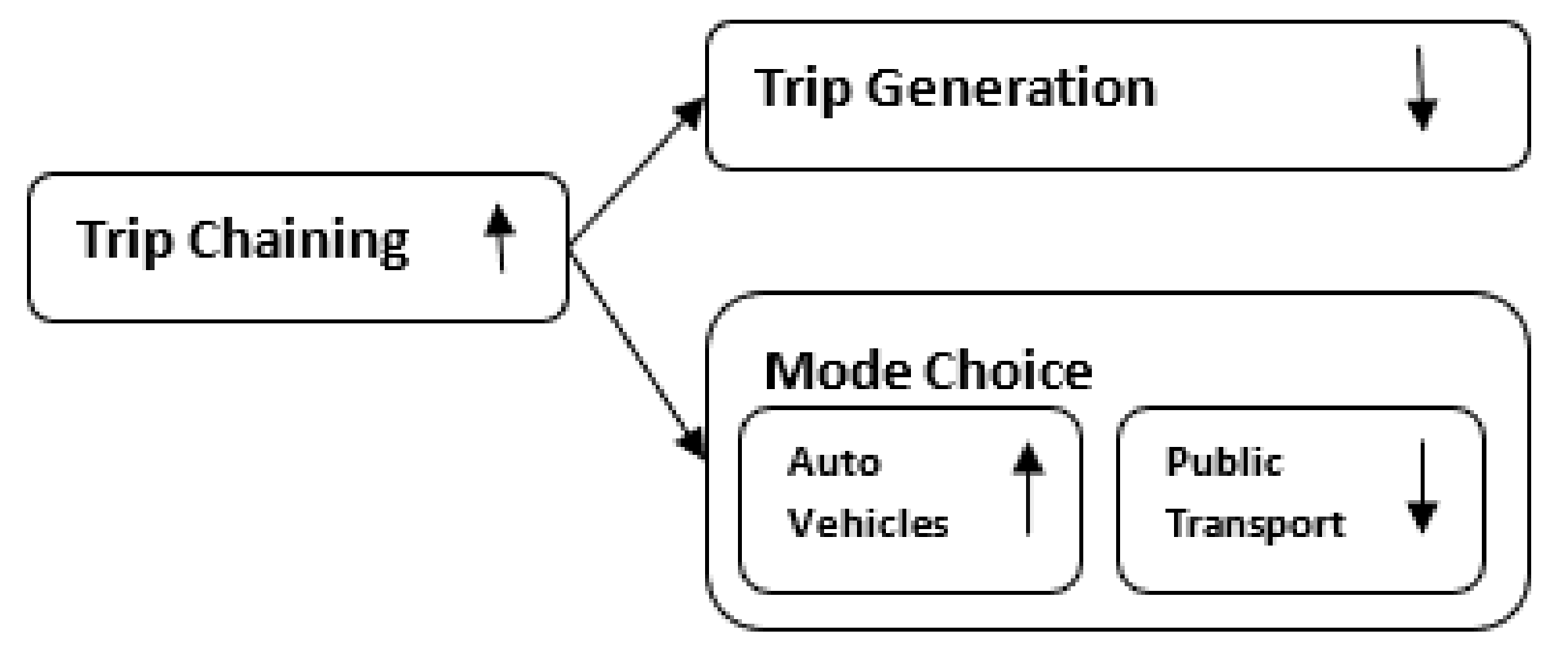
Research also shows there are relationships among trip generation, mode choice and trip chaining (
Figure 1). The term “trip chaining” is defined as stopping at one or more intermediate locations during a trip from an origin to a destination.
On the interaction between trip generation and trip chaining, mixed land use creates opportunities for increasing numbers of pass-by and multipurpose trips and directly reduces trip generation [
24]. A pass-by trip is a trip to a land use because of passing the land use while travelling to another destination.
On the interaction between mode choice and trip chaining, as individuals move from a simple tour to an increasingly more complex tour, the likelihood of using public transport decreases with the increasing number of links in the chain [
16]. A ‘tour’ or a ‘trip chain’ is a set of consecutive trips that begin from a location and return to that location to accomplish a primary activity with none, one, or more intermediate stops of any duration to fulfil a number of secondary activities through travel.
In practice, trip chaining studies use the multinominal logit model for modelling [
11], while the bivariate ordered probit model [
10] and ordered probit model [
13,
16] are also used. Regression analysis [
12,
25] has also been used for better insight into trip chaining behaviour and individuals’ travel patterns.
Finally, most studies agree that the formation of complex trip chains is related to socioeconomic, demographic and urban form characteristics [
10,
11,
12,
13]. Specific variables explored in the literature include household composition and life cycle stage, age, gender, marital status, income, employment status, car availability, residential density and density of transit stops.
Among the most accepted modelling techniques for each of trip generation, mode choice and trip chaining, (multiple) regression analysis is the only model structure which can be applied for all steps. Similarly, the socioeconomic, demographic and urban form characteristics are influential in all of the trip generation, mode choice and trip chaining stages.
Consequently, multiple regression analysis is selected as the model structure for this research while socioeconomic, demographic and urban form characteristics are used as the independent variables for model development.
3. Model Structure
Regression analysis is the most widely used framework for trip generation, mode choice and trip chaining modelling in the literature [
4,
12,
18,
22,
25]. The mathematical model structure for predicting private car trip generation for a land use can be expressed as follows:
where:
is private car trip generation,
and
are socioeconomic, demographic and urban form related indices respectively,
,
and
are coefficients related to socioeconomic, demographic and urban form indices respectively and
is a constant.
In Equation (1), the number of private car trips generated per unit of the land use is the model’s dependent variable to link the estimated trip generation and the land use characteristics, where any of the land use characteristics can be used as the unit. It is noted that the model was developed for private car traffic generation to include mode choice in the model structure. This type of model is known as a direct demand model because it does both trip generation and modal split functions simultaneously.
The percentage of trip generation, for which the target land use was the primary purpose of the trip, was used to apply the trip chaining effect on trip generation and mode choice. The following formula was used to determine the model’s dependent variables.
where:
is the private car trip generation per unit of land use indicator,
is the private car trip generation,
is the percentage of the trip generation for which the target land use was the primary purpose of the trip and
u is the land use indicator (e.g., gross floor area of building).
As Equation (2) shows, the effect of trip chaining has been considered by isolating the private car trip generation, for which the land use was the primary purpose of the trip, since only the non-chained trips constitute the additional traffic on the adjacent road. It is noted that other effects of trip chaining, such as pass-by trips and diverted linked trips, have not been examined in this research.
The applied regression model in this research is shown below:
where:
is as described in Equation (2) and the other parameters are as specified in Equation (1).
4. Data Collection
To develop independent variables for model calibration, socioeconomic, demographic and urban form related information at a suburb scale was collected since data at a suburb scale can show differences in transport features because the socioeconomic, demographic and urban form characteristics vary from one suburb to another. Traffic analysis zones were not considered in this research because they are not linked to socioeconomic, demographic and urban form characteristics and, consequently, are not able to demonstrate variations in them.
To develop socioeconomic, demographic and urban form related indicators, census data were used as it can provide data at a suburb level. However, direct application of the raw socioeconomic and demographic data such as age, gender and income cannot show socioeconomic and demographic differences between suburbs. Specific indicators for each of the proposed independent variables were created.
Table 1 shows the indicators used to develop socioeconomic, demographic and urban form related indices.
In
Table 1, the residential density of an area refers to the actual density (not proposed density) of dwelling units (i.e., trip generators), while non-residential density is the actual density of other land uses (i.e., trip attractors) in that area.
The average distance to transit (T) in each suburb was calculated by using the geographic coordinate data of public transport stop or station in the Hobart region combined with Hobart’s cadastral and road network maps in ArcGIS software. The distance from each lot in the Hobart area to the nearest public transport stop or station was calculated and then the average of the distances calculated for each suburb was applied as the average distance to transit indicator.
Table 2 shows the value of socioeconomic, demographic and urban form indicators for each suburb.
To assess the appropriateness of the indicators for use in the model, a correlation analysis was undertaken in SPSS software. The results of the correlation analysis for demographic indicators show there is a correlation between gender ration (G) and household Size (HS) at the 0.05 level of significance. Consequently, it was considered that either a function of average age (A) and gender ratio (G) or a function of average age (A) and household size (HS) should be used as the demographic index.
Similarly, of the socioeconomic variables, there was a correlation between employment ratio (E) and household income (HI) which is significant at the 0.05 level. As a result, either a function of car ownership (CO) and employment ratio (E) or a function of car ownership (CO) and household income (HI) was used as the socioeconomic index for model development.
Finally, of the urban form variables, there was a high correlation between residential density ratio (R) and distance to transit (T) at the 0.01 level of significance. As a result, a function of population density (P) and distance to transit (T) or a function of population density (P) and residential density ratio (R) was used as the urban form index for model development.
Ultimately, the independent variables for use in model development were as follows:
Different combinations of the indicators were created for use as socioeconomic, demographic and urban form related indices in the models. These combinations included multiplication and division of the selected indicators as well as each of the indicators individually and its reverse form, which resulted in 14 configurations of indicators for each of the socioeconomic, demographic and urban form categories.
As the next step, trip generation, mode choice and trip chaining data and general information related to existing LDCCs were collected to develop dependent variables for model calibration. The minimum sample size was considered to be 15 sites as James et al. [
26] suggests at least five samples for each independent variable to create an appropriate multiple regression model.
To collect trip generation, mode choice and trip chaining information, 15 LDCCs were selected randomly from a list of LDCCs in Hobart and Glenorchy City councils. The selected sites were in 11 different suburbs with an average population of 5540. This number of suburbs provides variations of socioeconomic, demographic and urban form characteristics and their influence on the trip generation rate of LDCCs to be tested properly by the proposed model.
The dependent variables were calculated by applying the data associated with LDCCs’ trip generation, mode choice and trip chaining data as well as the number of staff and the number of children in each LDCC. The floor area of each LDCC was not used to develop the dependent variables due to the lack of available information.
LDCCs’ trip generation, mode choice and trip chaining data collection were conducted on a typical Tuesday, Wednesday or Thursday during good weather conditions to capture the high end of typical weekday traffic. Data collection was avoided during school holidays to achieve accurate trip generation data for model development.
On the day of a given survey, the LDCC’s director was asked to provide information on the actual number of staff and children who attended the LDCC on that day. For trip generation data, traffic counts were conducted at the driveways of all the selected LDCC sites for the morning peak period between 7:30 a.m. and 9:00 a.m. The number of private cars going in and coming out of the LDCC was counted during the traffic survey.
Trip chaining data were collected through a customer interview undertaken in the afternoon of the same day of the traffic count at the LDCC when the parents were picking up their children. This was because parents were likely to be in a hurry during the morning drop off and may not be able to answer questions properly. The afternoon allowed interviewers to ask the questions in a more relaxed environment.
Interviews were conducted between 3:30 p.m. and 6:00 p.m., during the peak period of collecting children. Notification was also sent to the parents a week before the scheduled survey date to inform them about the interview. To avoid interruption to the centre’s business, parents and the centre’s staff (including the centre’s director) were asked on their way out of the centre what their next destination was after setting down their child on the day of the survey.
The average response rate to the interviews ranged from 65.4% to 94.6% per site with an average of 77.4% meaning the interview data can show the overall effect of trip chaining and the modal split of the LDCCs to an acceptable level.
To determine the effect of trip chaining, it was assumed that only the trips with home as the next destination after visiting the LDCC would be the trips for which the LDCC was their main purpose. Therefore, these trips were added to the number of staff who participated in the interview to identify the total trips to the LDCC without chained trips. The total was then divided by the total number of interviews to identify the percentage of total trips with the LDCC as the main destination.
The results of the traffic survey show that morning peak hour for LDCCs in the Hobart region predominantly occurred between 8 am and 9 am. The customer interviews at the selected LDCCs showed that most of the parents go to work after leaving their children at the LDCC (average 73.5%), while home is the next popular destination (average 14.7%). The average percentage of the trips to LDCCs without pass-by trips was 32.7%, ranging from 19% to 44% by site.
The dependent variable values for each surveyed site were calculated by applying Equation (2) and using the private car trip generation and trip chaining information as well as the number of children and number of staff at the surveyed LDCCs.
Table 3 shows the dependent variable values for each surveyed site (i.e., private car trip generation per unit of the site indicator associated with a mode of transport), which were used to calibrate the final model. In
Table 3,
means private car while
and
refers to each LDCC’s number of children and number of staff, respectively.
5. Model Calibration
Two different sets of multiple regression equation models were developed for private car traffic generation: one for trips per number of staff and one for trips per number of children.
The independent variables for developing the models based on Equation (3) were socioeconomic, demographic and urban form indices. Correlation analysis was also undertaken for different combinations of the independent variables to ensure that variables with a relationship were not used in model development. On this basis, a total of 1599 different models were developed for each trip generation classification: 1599 models for private car trip generation per number of staff and 1599 models for private car trip generation per number of children. The model with the highest coefficient of determination, R2, was selected as the best model for each trip generation classification.
To evaluate the performance of the above models, another two regression equation models were also developed using the conventional method of trip generation estimation. The mathematical model structure for developing the later models was as follows:
where:
is the private car trip generation per unit of LDCC indicator,
u is the LDCC indicator (i.e., either number of staff or number of children of the LDCC),
is the coefficient related to
u and
is a constant.
The results of the models based on Equation (3) for modelling trip generation are trip generation per one staff member or child. Consequently, the number of staff or children associated with the LDCC was multiplied in the result of the model to provide the total private car trip generation associated with the LDCC. The estimated private car trip generation by any of the developed models was rounded up to the next integer.
All the models were developed using SPSS software. The estimated private car trip generation values from each model were compared with the actual private car trip generation data by undertaking the two sample Kolmogorov–Smirnov (TSKS) test. The null hypothesis of the TSKS test is that the samples are drawn from the same distribution. The results of TSKS tests together with other statistical tests provided a baseline to evaluate whether the models based on Equation (3) or the models based on the conventional method of private car trip generation estimation lead to more accurate results, which are closer to reality.
6. Results
A comparison between the models created based on Equation (3) and the conventional method shows that the number of children as the LDCC’s indicator performs better for estimating private car trip generation for both modelling methods.
In addition, the results of the TSKS tests show that the distributions of the results from all models are not the same as the distribution of the trip generation values, which were used to calibrate the models.
Approximately two-thirds of the results of the models based on Equation (3) for estimating private car trip generation provide closer results to the actual private car trip generation values (i.e., ) and the difference between those models and shows smaller variation compared to the conventional models.
Based on the above results, it can be concluded that neither modelling method can estimate private car trip generation equal to . However, the models using Equation (3) for private car trip generation estimation perform relatively better compared to using conventional variables for private car trip generation estimation.
Following are the detailed results of the model predicting private car trip generation per child, as an example.
Private Car Trip Generation per Child (TGpc)
Using the conventional method of trip generation estimation, the following model (named
) was the best linear regression model for estimating private car trip generation of LDCCs based on the number of children:
Regarding the model based on Equation (3) for estimating private car trip generation (named
), a comparison among the models shows that the best-fitted regression equation to the
data was:
In addition, the following two models provided closer results to the actual private car trip generation values (i.e.,
), although they have lower R
2 values.
Regarding models developed based on Equation (3), T or R × P appeared to be the best indicator of urban form.
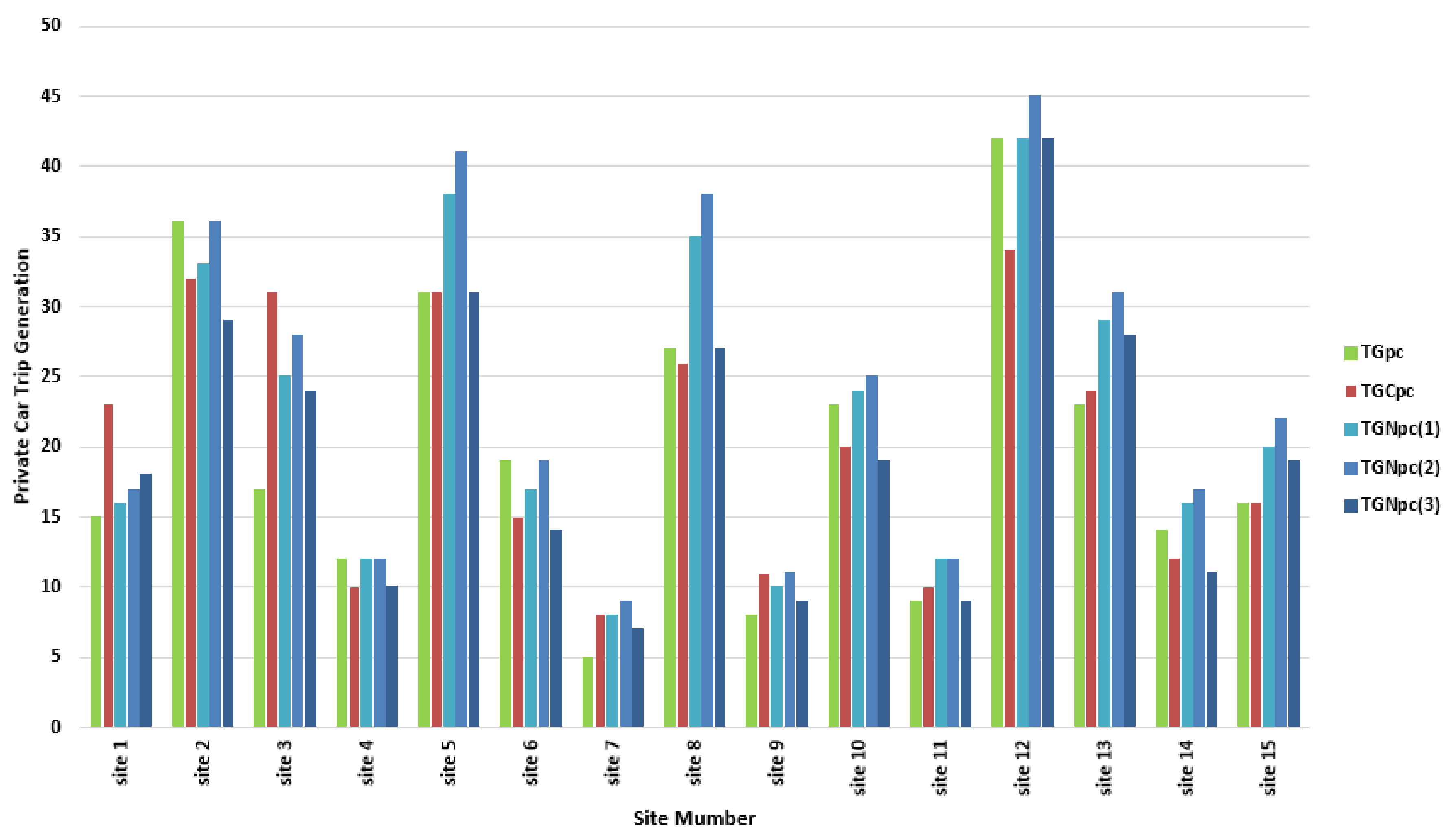
Figure 2 and
Table 4 show the private car trip generation estimation for each site based on the above equations, with the variation from the
value shown in brackets.
A review of the results in
Table 4 shows that the R
2 of the conventional model was higher than the models based on Equation (3) while the results of the models based on Equation (3) show less difference on
. In addition, the results of the conventional model were better than the models based on Equation (3) only for four of the 15 sites. Consequently, it can be concluded that the models based on Equation (3) predominantly provide closer results to
whereas the conventional model shows higher R
2.
7. Conclusions
Findings from this research show that using socioeconomic, demographic and urban form indices to estimate private car trip generation of LDCCs will provide relatively better results by reflecting the overall impact of socioeconomic, demographic and urban form differences among suburbs on LDCCs’ private car trip generation. This research provides evidence-based recognition that socioeconomic, demographic and urban form indices at a suburb scale can be used as traffic and transport attributes in traffic and transport studies. However, the research was not able to identify the best form of the indices.
The methodology of this research will provide a useful tool for professionals to undertake sensitivity studies to gain a better understanding of the impact of specific socioeconomic, demographic and urban form characteristics on a traffic demand attribute.
Based on the results of this research, other variables can be further investigated to identify the best configuration of the indices. Developing models by using other modelling techniques such as non-linear regression based on the proposed indices in this research can also be examined. Similar models for other modes of transport can be developed based on the approach and the indices applied in this research to recognise if the best-fitted independent variables for socioeconomic, demographic and urban form characteristics are consistent across different modes of transport. Models for other land uses based on the approach and the indices in this research can distinguish whether independent variables are unchanged across models for different land uses. Finally, based on the approach of this research, similar models should be developed for other cities to test whether such models are transferable across cities.


