Radar Detection-Based Modeling in a Blast Furnace: A Prediction Model of Burden Surface Descent Speed

Abstract

The distribution of burden layers is a vital factor that affects the production of a blast furnace. Radars are advanced instruments that can provide the detection results of the burden surface shape inside a blast furnace in real time. To better estimate the burden layer thicknesses through improving the prediction accuracy of the burden descent during charging periods, an innovative data-driven model for predicting the distribution of the burden surface descent speed is proposed. The data adopted were from the detection results of an operating blast furnace, collected using a mechanical swing radar system. Under a kinematic continuum modeling mechanism, the proposed model adopts a linear combination of Gaussian radial basis functions to approximate the equivalent field of burden descent speed along the burden surface radius. A proof of the existence and uniqueness of the prediction solution is given to guarantee that the predicted radial profile of the burden surface can always be calculated numerically. Compared with the plain data-driven descriptive model, the proposed model has the ability to better characterize the variability in the radial distribution of burden descent speed. In addition, the proposed model provides prediction results of higher accuracy for both the future surface shape and descent speed distribution.

1. Introduction

Burden layer distribution plays an important role in the internal state of a blast furnace (BF) because different layer distributions lead to different permeabilities, which in turn affect the temperature distribution and the height and shape of the cohesive zone [1,2]. For the charging mechanism of a rotating chute in bell-less charging, the shape of the burden surface can be regarded as symmetric; therefore, the radial profile of the burden surface (BSRP) can be studied. Two main factors that affect the BSRP directly are burden charging and burden descending. Modeling of the charging process and burden stacking behavior has been addressed in our previous research [3]. As a continuation of the previously established model, a model of the descent speed distribution along the burden surface radius (BSRD) is proposed in this research.

Burden descent models can be divided into three main categories: geometric profile models [4,5], continuum models [6,7] and discrete element method (DEM) models [8]. Geometric profile models have simple mathematical descriptions. This computational simplicity makes geometric profile models appropriate for online calculation scenarios. A recent review article [5] noted that the model that adopts a data-driven technique to approximate the nonuniform descent speed of the burden surface exhibits a better performance than that of other geometric profile models. However, the drawback of this type of model is also obvious: geometric profile models rely on empirical parameters that may be time-variant during BF production. The DEM models have the most complex form among these three types of models. In small-scale simulations, the DEM can provide highly-accurate results with abundant details. However, in BF burden simulations, the millions of simulated particles increase the computational complexity, making it impossible to perform real-time predictions. Compared to the above-mentioned two types of models, continuum models have moderate complexity and accuracy. With the development of computer hardware, optimized continuum models can eventually be adopted in real-time computation [9].

The differences among continuum models are mainly found in their different corresponding governing equations. Such models fall into three main categories: potential flow models (PFMs) [9,10], kinematic models (KMs) [11,12] and viscous flow models (VFMs) [13]. PFMs have simple governing equations. Their computational complexity is relatively low; only the effects of the geometrical boundaries on the descending dynamic can be reflected. VFMs characterize solid flow behaviors considering the effects of the gas phase and friction at the geometrical boundaries, hence providing highly accurate results of the burden descent behavior. However, the geometrical boundaries in the BF bottom are affected by the shape of the deadman zone, which needs to be given a priori [7]. In practice, this shape is challenging to detect. Compared with PFMs and VFMs, KMs are promising in terms of exhibiting high performance in modeling the movement of the solid burden in the bulk area of a BF (i.e., the throat and upper stack region of the BF) not only because they can reproduce experimental data quite accurately [14] but also because they are structured to include only one model parameter. This type of model may be less affected by the possible inaccuracy of this parameter and hence more robust.

Due to the harsh environment inside operating BFs, it is difficult for conventional sensors to detect the burden surface directly. Therefore, researchers have adopted scaled experiments [4,6], computational fluid dynamics (CFD) simulations [7] and DEM simulations [8] for analysis. Industrial radar systems can detect the burden surface shape of an operating BF in real time [15,16]. Hence, the corresponding BSRD can be obtained. Although the inner state of the burden descent field beneath the burden surface cannot be detected by radar, deviations introduced by simulation methods can be largely reduced.

In our former work, a prediction model of burden charging was constructed [3]. In this research, a kinematic modeling-based prediction model of BSRD was proposed. This model can serve as a submodel for predicting the burden descent and be embedded in the former prediction model of burden surface shape to further improve the overall prediction accuracy. The data used in the parameter identification and model verification stages were from the detection results of a real operating BF detected using a mechanical swing radar (MSR) system and are not from the results of other simulations or experiments [3,17].

2. Measurement Results

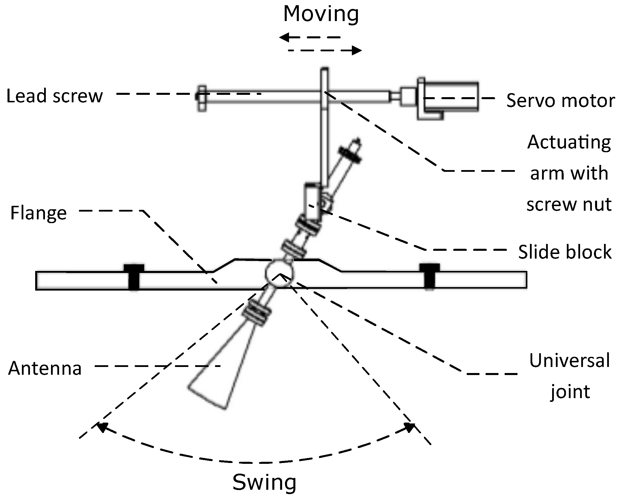
2.1. Instrument Settings

To obtain the real-time BSRP, an MSR was installed on top of a BF [17]. There are two obvious advantages of this system adopted in BF gauging scenarios. First, the operation mode of this radar system is similar to that of laser scanning devices. Therefore, the system can detect the height of the burden surface along a radius at a high accuracy. Moreover, the measurement system uses a wavelength longer than that of a laser, enabling this system to detect features within the heavy dust environment inside the BF. Second, compared with the radar array system [15] installed on top of the furnace, the MSR scans and detects the surface height more densely along the radial direction of the burden and thus provides detection results with higher azimuthal resolution.

In the measurement process, the radar antenna is driven by a mechanical servo system to swing periodically along the radial direction of the burden surface, while the radar measures the burden height of the corresponding scanning positions. The time-variant BSRP can thus be obtained. The radar mounted on top of the BF is illustrated in Figure 1.

As shown in Figure 1, the setting of an absolute coordinate $C_A$ and a relative coordinate $C_R$ are inherited from our former model [3] for consistency. Both $C_A$ and $C_R$ have vertical axes along the BF center from bottom to top and horizontal axes along the BF radius from center to wall. $C_A$ is set at a fixed height, where the vertical distance between $C_A$ and the MSR is denoted as $H_1$. $C_R$ varies with the burden surface radius, where the lowest points of the BSRP remain on the horizontal axis.

The radar adopts the frequency-modulated continuous wave principle and operates at frequencies of 24–$26\mathrm{GHz}$. The range resolution is approximately $0.09\mathrm{m}$. The mechanism of the radar servo system is demonstrated in Figure 2.

Before being mounted on the BF top, the MSR was calibrated in a pilot plant and initialized on the top of the BF in open state [17]. The measured BF has a diameter of $8.5\mathrm{m}$ in the throat region. Ten to twelve detection positions were evenly distributed along the BF radius. In practical measurement, the MSR scanned the burden radius successively at a scan rate of $1/60\mathrm{Hz}$. The BF database system were used to record both the burden charging settings and the measurement results of the MSR synchronously. A sample of the record was presented in Table 1 of [3]. In this research, the charging information in the record were used to label and screen out the noncharging periods. Measurement results of the MSR in the extracted noncharging periods were used.

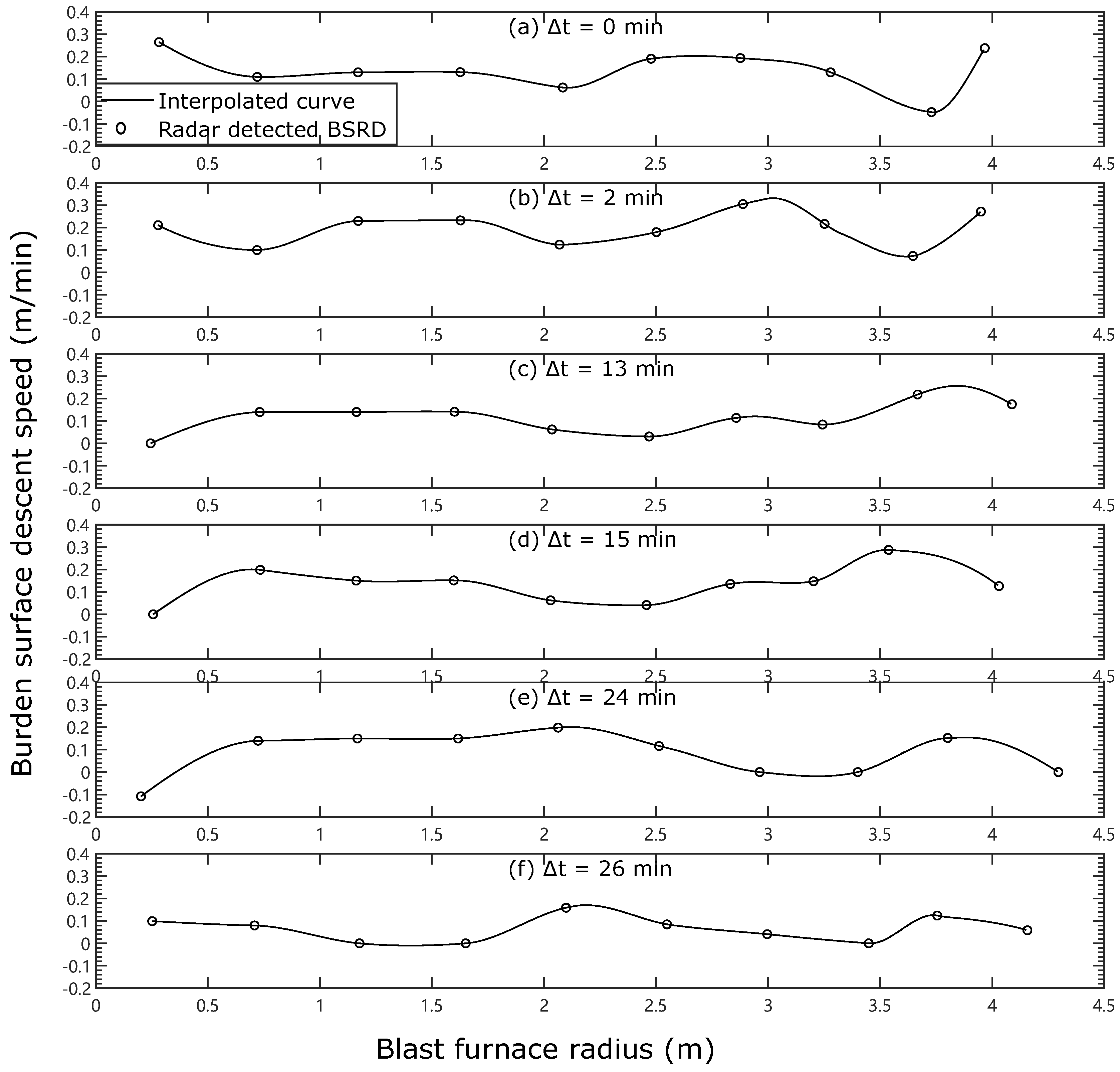
2.2. Detection Results

The detection results in Figure 3 represent the variation in the BSRDs within half an hour. The detection time of the sample in Figure 3a is set as a time reference. $\mathrm{\Delta }t$ in each subfigure denotes the timespan between the detection time of a sample and the time reference. In addition, the results in Figure 3a,b, Figure 3c,d, and Figure 3e,f are three pairs of neighboring samples obtained within three noncharging periods.

Two features of the time-variant BSRDs can be observed and generalized:

• The BSRDs are nonuniform.
• There are similarities between the shapes of the time-adjacent BSRD samples.

Figure 3 clearly shows that all of the BSRDs are nonuniform. Further, there exists significant variation in the descent speed between neighboring detection positions. As shown in Figure 3e, the distribution of the descent speed for $r\in [2,3]$ has a variation of $0.2\mathrm{m}/\min$. The primary cause of this phenomenon is that the radial distribution of the volumetric consumption in the bottom section of the BF is uneven. Additionally, the geometric shape of the furnace body (e.g., the inclination of the furnace wall) may have effects on the BSRD.

For the second feature, the similarities are manifested on two levels. For distributions within a pair (e.g., Figure 3a,b), there is a strong similarity both in local shape and global trend. Therefore, the variation rate of the descent distribution is slower than the scanning rate of the radar detection. For BSRDs of neighboring pairs (e.g., Figure 3b,c), the similarities were found in the global trend and at local intervals. More specifically, for $r\in [1,3]$ in Figure 3b,c and $r\in [0,1.5]\cup [3,4.5]$ in Figure 3d,e, the descent distributions are similar. However, for $r\in [1.5,3]$ in Figure 3d,e and $r\in [0,1]\cup [3,4.5]$ in Figure 3b,c, the variations are obvious.

In addition, there are negative values in the BSRDs, as shown at $r=3.75$ in Figure 3a and $r=0.2$ in Figure 3e. This outcome implies that burden ascend in the corresponding locations. We think that the transient ascent of the burden in local radial positions is acceptable. First, the descent speed at $r=3.75$ in Figure 3b and $r=0.2$ in Figure 3f are both positive, which means burden ascents in Figure 3a,e are transient. Further, comparing the distribution of the BSRD at $r\in [0,1]$ in Figure 3e,f, with the variation of detected descent speed from negative to positive at $r=0.2$ from Figure 3e to Figure 3f, the detected descent speed at $r=0.7$ decreases from $0.14\mathrm{m}/\min$ to $0.09\mathrm{m}/\min$. Since the movement of the burden particles is affected by the geometrical shape of the burden surface, the tumbling of burden particles from peaks to valleys on the burden surface is one possible cause of the transient negative values in the BSRDs. Additionally, although rotational symmetry of the burden distribution is assumed in a practical sense, local abnormalities (i.e., negative descent speed in local burden radius) in the results of the detected BSRDs may suggest that there is a rotational asymmetry in the local burden distribution to some extent.

Notably, the variation rate of the BSRD is slower than the MSR scan rate. If the mechanism of descent variation is modeled, a prediction model for BSRD can be further designed based on the burden descent mechanism and the radar-detection-driven technique.

3. Model Description

3.1. Kinematic Modeling Mechanism

The movement of burden particles in the throat and upper stack region was considered, as shown in Figure 4.

Since the decrease in volume originates from the chemical reaction of the burden materials in the lower part of the stack region where the burden temperature reaches $1100{}^{\circ }\mathrm{C}$ [1], the height of $C_A$ is used as the separatrix, and it is assumed that there is no decrease in volume in the region $h>0$. Then, the phenomenon of burden surface descent results from the driving of burden volumetric consumption in the $h<0$ region and the transmitting of burden descent by solid burden particles in the $h>0$ region. The physical assumptions are stated below:

Assumption 1.

The movement of burden particles in the $h>0$ region of $C_A$ is solely driven by gravity.

Assumption 2.

A decrease in the burden volume occurs in the $h<0$ region of $C_A$, and there is no decrease in the volume in the $h>0$ region.

Denote the velocity field of the burden in the $h>0$ region of $C_A$ as $V(r,h)=\left(v\right(r,h),u(r,h\left)\right)$. As demonstrated in Figure 4, for an arbitrary burden particle I, based on Assumption 1, its movement depends on the movements of neighboring particles II and III below. Without loss of generality, assuming that the vertical component of the descent speed of particle III is greater than that of particle II, particle I will move towards particle III’s location. This behavior can be described by a simplified linear relation as Equation (1) [12]:

$$v(r,h)=-B\frac{\partial u(r,h)}{\partial r}$$

(1)

where B is the kinematic constant. Under Assumption 2, since the burden in the $h>0$ region undergoes no decrease in volume, the incompressible condition holds for solid burden particles, stated as Equation (2):

$$\frac{\partial v(r,h)}{\partial r}+\frac{\partial u(r,h)}{\partial h}=0$$

(2)

Substitute Equation (1) into Equation (2) to obtain the governing equation of the KM [18] for the burden descent behavior, stated as Equation (3):

$$\frac{\partial u(r,h)}{\partial h}=B\frac{{\partial }^{2}u(r,h)}{\partial r^2}$$

(3)

Consider a case of solid flow in the two-dimensional rectangular region $D=\left\{\right(r,h\left)\right|0\le r\le R,0\le h\le H\}$, where R is the burden radius. There is a consumption source formulated in the form of a unit-impulse function $C(·)$ with diameter $d(d\ll R)$ on the lower boundary at $(R/2,0)$, as defined in Equation (4).

$$C\left(r\right)=\left\{\begin{array}{c}1/d,\left|r\right|\le d/2\hfill \\ 0,\left|r\right|>d/2\hfill \end{array}\right.$$

(4)

Then, the descent dynamics of the burden particles can be described by a boundary value problem of a partial differential equation (PDE), as in Equation (5).

$$\left\{\begin{array}{cc}\frac{\partial u(r,h)}{\partial h}=B\frac{{\partial }^{2}u(r,h)}{\partial r^2},\hfill & r\in [0,R],h\in (0,H]\hfill \\ u(r,0)=QC(r-\frac{R}{2}),\hfill & r\in [0,R]\hfill \end{array}\right.$$

(5)

where Q is the volumetric flow rate. The results of Tuzun’s work [19] show that the distribution of burden descent speed, i.e., the solution of Equation (5), can be described as Equation (6):

$$u(r,h)=\frac{Q}{\sqrt{4Bh}}\exp \left[-\frac{{(r-R/2)}^2}{4Bh}\right]$$

(6)

Denote by $\mathrm{\Phi }(·)$ a Gaussian function, as follows:

$$\mathrm{\Phi }\left(r\right)=\frac{1}{\sigma }\exp \left(-\frac{r^2}{{\sigma }^2}\right)$$

(7)

Because $\mathrm{\Phi }\left(r\right)$ is continuous and bounded, Equation (6) is identical to the solution of the Cauchy problem in Equation (8) when $\sigma \to 0$ [20].

$$\left\{\begin{array}{cc}\frac{\partial u(r,h)}{\partial h}=B\frac{{\partial }^{2}u(r,h)}{\partial r^2},\hfill & r\in (-\infty ,\infty ),h\in (0,H]\hfill \\ u(r,0)=Q\mathrm{\Phi }(r-\frac{R}{2}),\hfill & r\in (-\infty ,\infty )\hfill \end{array}\right.$$

(8)

It follows that the approximate solution of the boundary value PDE problem in Equation (5) can be obtained by solving the corresponding Cauchy problem in Equation (8), and $C\left(r\right)$ can be approximately replaced by $\mathrm{\Phi }\left(r\right)$ on the precondition of $d\ll R$. Additionally, for any fixed h, Equation (6) is also a Gaussian function.

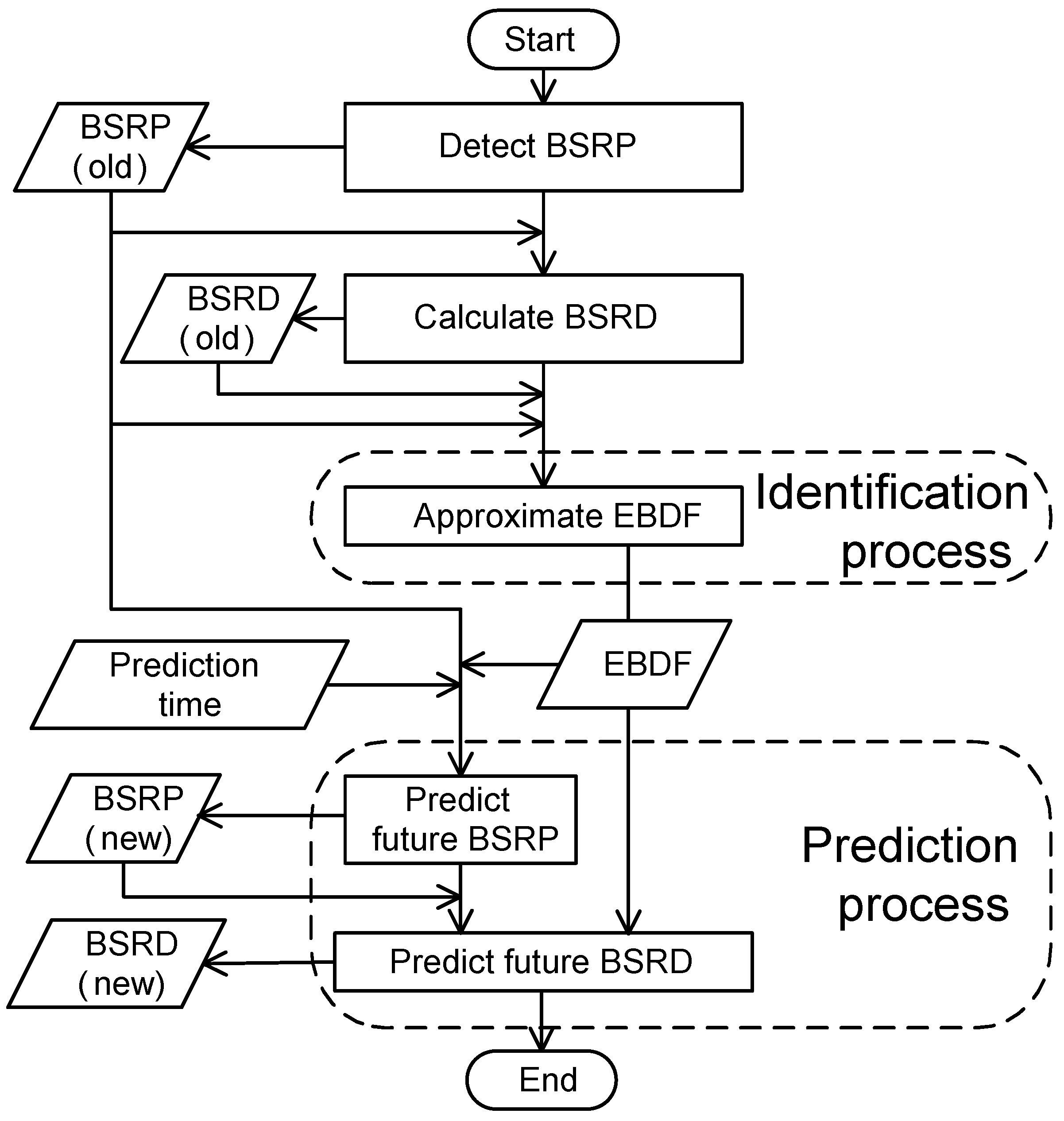
3.2. Prediction Model

The burden surface descent results from the descent of the burden beneath the surface. However, calculating the real field of burden radial descent speed from the detection results of BSRD is an ill-posed inverse problem because different distributions of the field may correspond to the same BSRD. We introduce the notion of an equivalent radial burden descent speed field (EBDF). The EBDF is an approximated solution of the governing equation of the problem, in which the equivalence between the values on the upper boundary of the EBDF and the measurement output of the BSRD is guaranteed. In the proposed prediction model, EBDF is identified in an approximation approach based on the detection results of the BSRD. Then, a future BSRD can be calculated with the obtained EBDF and other input parameters, including the prediction time and initial state of the BSRP. The flow of the model is demonstrated in Figure 5.

Prediction model assumptions:

Assumption 3.

The distribution of burden descent speed in the $h>0$ region of $C_A$ remains constant during the time of the model prediction.

Assumption 4.

The effects of the inclination of the furnace wall on the burden descent in the stack region can be regarded as those of the equivalent consumption sources located at $h=0$ of $C_A$.

Assumption 5.

The BSRD equals the descent speed distribution at $h=0$ of $C_R$.

In $C_A$, let $u_s(r_i,h_i)(i=1,\dots ,n)$ be the obtained discrete BSRD. $h_A$ is the vertical distance between two horizontal axes, $C_A$ and $C_R$, and varies with the location of $C_R$; $h_A$ is calculated as $h_A=min\left\{h_i\right\}(i=1,\dots ,n)$. Then, under Assumptions 4 and 5, $u(r_i,h_A)=u_s(r_i,h_i)$ holds. The solution domain of the radial burden descent speed can be expressed as Equation (9), referring to $C_A$, as shown in Figure 6.

$$D_s=\left\{(r,h)\right|0\le r\le R,0\le h\le h_A\}$$

(9)

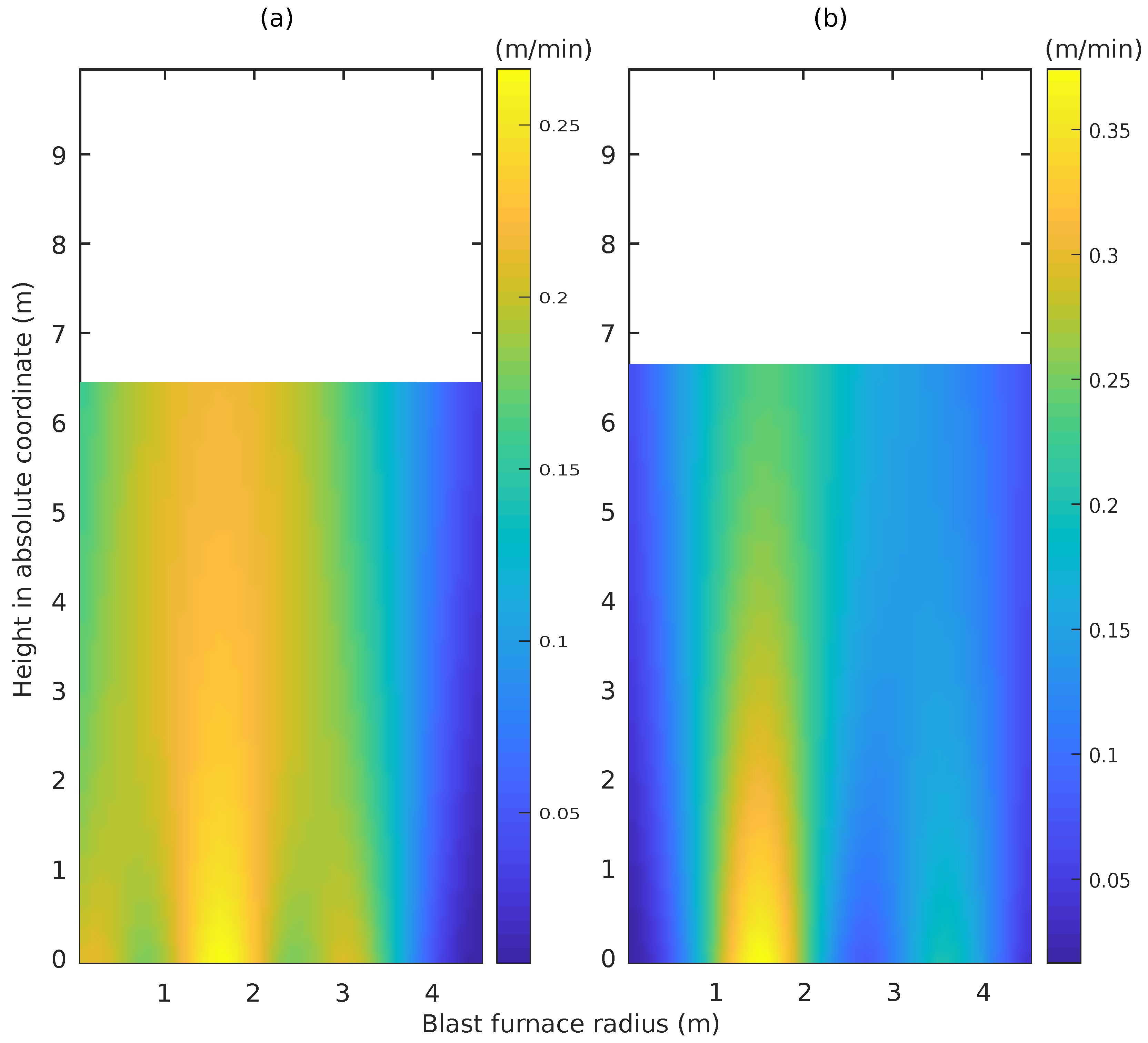
3.2.1. Approximation of Burden Vertical Descent Speed Field

The problem of calculating the EBDF can be formulated into solving a PDE problem stated as Equation (10) with discrete measurement output stated as Equation (11):

$$\frac{\partial u(r,h)}{\partial h}=B\frac{{\partial }^{2}u(r,h)}{\partial r^2},r\in [0,R],h\in [0,h_A]$$

(10)

$$u(r_i,h_A)=u_s(r_i,h_i),(i=1,\dots ,n)$$

(11)

Furthermore, because the consumption source in the Cauchy problem in Equation (8) and the radial distribution of descent speed at a given height Equation (6) are both Gaussian functions, equivalent consumption sources ${\mathrm{\Phi }}_j\left(r\right)$ located at $h=0$ of $C_A$ can be formulated in the form of a Gaussian function as Equation (12). For each source, $r_j$ specifies its position along the burden radius from the BF center to the wall, ${\sigma }_j$ is the shape parameter of the Gaussian function and characterizes its own nature of consumption.

$${\mathrm{\Phi }}_j\left(r\right)=\frac{1}{{\sigma }_j}\exp \left[-\frac{{(r-r_j)}^2}{{{\sigma }_j}^2}\right],r_j\in [0,R]$$

(12)

Corresponding to the first feature of the BSRD concluded from Figure 3, the nonuniformity of the distribution can be characterized by arranging equivalent consumption sources at different radial positions. The synthesizing impact of multiple equivalent sources at $h=0$ can be expressed in an integrated form, the linear combination of Gaussian functions along $h=0$, to approximate the descent speed distribution at $h=0$, as Equation (13):

$$u(r,0)=\sum _{j=1}^m{Q}_j{\mathrm{\Phi }}_j\left(r\right)$$

(13)

where $Q_j$ is the parameter characterizing the strength of each consumption sources. Based on the setting of boundaries in the Cauchy problem in Equation (8), a boundary value PDE problem can be formulated as Equation (14):

$$\left\{\begin{array}{cc}\frac{\partial u(r,h)}{\partial h}=B\frac{{\partial }^{2}u(r,h)}{\partial r^2},\hfill & r\in (-\infty ,\infty ),h\in (0,h_A]\hfill \\ u(r,0)={\sum }_{j=1}^m{Q}_j{\mathrm{\Phi }}_j\left(r\right),\hfill & r\in (-\infty ,\infty )\hfill \end{array}\right.$$

(14)

The EBDF can be calculated in two steps:

• Solve the boundary value problem defined by Equation (14).
• Use the discrete measurement output of the BSRD in Equation (11) to identify the unknown parameters $\{{\sigma }_1,\dots ,{\sigma }_m;r_1,\dots ,r_m;Q_1,\dots ,Q_m;B\}$ in the parameterized boundary value solution obtained in the first step.

First, for the boundary value problem defined by Equation (14), its solution has the form as follows [20]:

$$u(r,h)={\int }_{-\infty }^{+\infty }k(r-a,h)u(a,0)da$$

(15)

where

$$k(r,h)=\frac{1}{\sqrt{4\pi Bh}}\exp \left(\frac{-r^2}{4Bh}\right)$$

(16)

Substitute Equation (13) into Equation (15) to determine the following:

$$\begin{array}{ccc}\hfill u(r,h)& =& {\int }_{-\infty }^{+\infty }k(r-a,h)\sum _{j=1}^m{Q}_j{\mathrm{\Phi }}_j\left(a\right)da\hfill \\ & =& \sum _{j=1}^m{Q}_j{\int }_{-\infty }^{+\infty }k(r-a,h){\mathrm{\Phi }}_j\left(a\right)da\hfill \end{array}$$

(17)

Further, calculate the convolution on the right-hand side of Equation (17) by the Fourier transform:

$$\begin{array}{ccc}\hfill u(r,h)& =& \sum _{j=1}^m{Q}_j{\int }_{-\infty }^{+\infty }k(r-a,h){\mathrm{\Phi }}_j\left(a\right)da\hfill \\ & =& \sum _{j=1}^m{Q}_j\sqrt{\pi }{\int }_{-\infty }^{+\infty }\left\{\frac{1}{\sqrt{4\pi Bh}}\exp \left[\frac{-{(r-a)}^2}{4Bh}\right]\right\}\left\{\frac{1}{\sqrt{\pi }{\sigma }_j}\exp \left[\frac{-{(a-r_j)}^2}{{\sigma }_j^2}\right]\right\}da\hfill \\ & =& \sum _{j=1}^m\frac{Q_j}{\sqrt{4Bh+{\sigma }_j^2}}\exp \left[\frac{-{(r-r_j)}^2}{4Bh+{\sigma }_j^2}\right]\hfill \end{array}$$

(18)

Here, we obtain the parameterized boundary value solution, $u(r,h)$, which is referred to as the above-mentioned EBDF.

With the discrete measurement output of the BSRD in Equation (11), the following optimization problem in Equation (19) can be formulated. Then, the unknown parameters $\{{\sigma }_1,\dots ,{\sigma }_m;r_1,\dots ,r_m;Q_1,\dots ,Q_m;B\}$ can be identified by solving Equation (19).

$$minJ=\sum _{i=1}^n{\left[u(r_i,h_i)-u_s(r_i,h_i)\right]}^2$$

(19)

We named this prediction model the kinematic Gaussian model (KGM) based on the form of Equation (18), which is a linear combination of Gaussian functions. It should be noted that the setting of the geometrical shape of the solution domain has impacts on the identified values of the EBDF parameters. Due to the inclination of the furnace wall in the stack region, the width of the solution domain is less than the length of the BF radius at the height of $h=0$ referring to $C_A$. As shown in Figure 6, the length difference is labeled as $\mathrm{\Delta }R$. As indicated in Equation (12), the positions of the equivalent consumption sources cannot be identified to the values in $r\in [R,R+\mathrm{\Delta }R]$. Therefore, the actual descent effects of the burden in $r\in [R,R+\mathrm{\Delta }R]$ will be compensated by the effects of the equivalent consumption sources located in $r\in [0,R]$. Hence, the identified values of the EBDF parameters are biased. This is one notable limitation of the purposed model.

3.2.2. Prediction of BSRD

Denote by f the function of BSRP with radial position variable r and time variable t. Let $f_{S0}$ and $f_{S1}$ be BSRP distributions referring to $C_A$ at time $t_0$ before and $t_1$ after the burden descent, respectively. Then, $(r_i,f_{S0}\left(r_i\right))(i=1,\dots ,n)$ are the discrete points on the BSRP referring to $C_A$ detected at time $t_0$. Given the calculated EBDF, $u(r,h)$, the future discrete BSRD at time $t_1(t_0<t_1)$, denoted as $(r_i,u_{S1}\left(r_i\right))(i=1,\dots ,n)$, can be calculated in two steps:

• Use $u(r,h)$ and $(r_i,f_{S0}\left(r_i\right))(i=1,\dots ,n)$ to predict the future discrete BSRP, denoted as $(r_i,f_{S1}\left(r_i\right))(i=1,\dots ,n)$.
• Use $u(r,h)$ and $(r_i,f_{S1}\left(r_i\right))(i=1,\dots ,n)$ to calculate the future discrete BSRD, $(r_i,u_{S1}\left(r_i\right))(i=1,\dots ,n)$.

In the first step, in $C_A$, let $h_{A0}=min\left\{f_{S0}\left(r_i\right)\right\}(i=1,\dots ,n)$. In addition, $f_{R0}\left(r_i\right)$ referring to $C_R$ corresponds to $f_{S0}\left(r_i\right)$ in $C_A$, as Equation (20):

$$f_{S0}\left(r_i\right)=h_{A0}+f_{R0}\left(r_i\right)$$

(20)

The physical relation between the burden stocklevel and burden descent speed can be formulated into an ordinary differential equation (ODE). Then, the first step can be formulated as solving the ODE initial value problem in Equation (21), and $f_{S1}\left(r_i\right)$ can be calculated using Equation (22).

$$\left\{\begin{array}{c}\frac{df(r_i,t)}{dt}=-u(r_i,f(r_i,t))\hfill \\ f(r_i,t_0)=h_{A0}\hfill \end{array}\right.$$

(21)

$$f_{S1}\left(r_i\right)=f(r_i,t_1)+f_{R0}\left(r_i\right)$$

(22)

The explicit solution of Equation (21) is difficult to obtain due to the complexity of $u(r_i,f(r_i,t))$. Here, instead, we prove that the numeric solution can be calculated. The existence and uniqueness of the solution can be guaranteed by Proposition 1 below (its proof is provided in the Appendix). Then, the future discrete BSRP, $(r_i,f_{S1}\left(r_i\right))(i=1,\dots ,n)$, can be calculated by classical numeric methods, such as the Runge–Kutta method.

Proposition 1.

Given a prediction time $t_1$, for arbitrarily fixed $r\in [0,R]$, there exists a unique solution of the initial value problem in Equation (21) on the interval $t_0<t<min(t_1-t_0,\frac{h_{A0}}{max\left|u\right(r,h\left)\right|})+t_0$.

In the second step, let $h_{A1}=min\left\{f_{S1}\left(r_i\right)\right\}(i=1,\dots ,n)$. Since $u(r,h)>0$, $f(r_i,t_0)>f(r_i,t_1)$,

$$\begin{array}{ccc}\hfill f_{S1}\left(r_i\right)& =& f(r_i,t_1)+f_{R0}\left(r_i\right)\hfill \\ & <& f(r_i,t_0)+f_{R0}\left(r_i\right)=f_{S0}\left(r_i\right)\hfill \end{array}$$

(23)

Furthermore,

$$\begin{array}{ccc}\hfill h_{A1}& =& min\left\{f_{S1}\left(r_i\right)\right\}\hfill \\ & <& min\left\{f_{S0}\left(r_i\right)\right\}=h_{A0}\hfill \end{array}$$

(24)

Hence, $(r_i,h_{A1})$ must be in the solution domain $D_s=\left\{(r,h)\right|0\le r\le R,0\le h\le h_{A0}\}$. Then, under Assumptions 3 and 5, the future discrete BSRD at $t_1$, $(r_i,u_{S1}\left(r_i\right))(i=1,\dots ,n)$, can be calculated as stated in Equation (25):

$$u_{S1}\left(r_i\right)=u(r_i,h_{A1})$$

(25)

Notably, as shown in Figure 3, there are cases of detected BSRD in which negative values of the local descent speed exist, whereas by Equation (18) and Equation (25), the predicted BSRD is globally nonnegative. Therefore, the proposed model cannot reproduce such BSRDs. Further, by Equation (19), when a BSRD that contains negative local values is adopted in identifying the model parameters, the approximation error of the EBDF will increase. This is another limitation of the proposed model.

4. Solution of Model Parameters

4.1. Identification of EBDF Parameters

Because 10–12 detection points of each scan on the BSRP are inadequate for identifying the parameters of the equivalent sources, $\{{\sigma }_1,\dots ,{\sigma }_m;r_1,\dots ,r_m;Q_1,\dots ,Q_m;B\}$, two BSRD samples obtained in one noncharging period were used in each calculation.

Let $t_1$–$t_2$, $t_2$–$t_3$, $t_4$–$t_5$ and $t_5$–$t_6(t_1<t_2<t_3<t_4<t_5<t_6)$ be four periods of radar scanning detections. As the first two and the last two periods are continuous in time, the MSR scans twice successively during $t_1$–$t_3$ and another two times during $t_4$–$t_6$. Then, $u_s^{\left(1\right)}(r_i,h_i^{\left(1\right)})$ and $u_s^{\left(2\right)}(r_i,h_i^{\left(2\right)})(i=1,\dots ,n)$ denote the calculated discrete BSRDs from the first and the last two successive scanning results, respectively. We refer to the above-described four periods of radar scanning data in one noncharging period as a data segment. Let

$$\begin{array}{ccc}\hfill h_1& =& min\{h_i^{\left(1\right)},(i=1,\dots ,n)\}\hfill \\ \hfill h_2& =& min\{h_i^{\left(2\right)},(i=1,\dots ,n)\}\hfill \end{array}$$

(26)

Then, the optimization objective, Equation (19), can be extended accordingly by introducing two weight coefficients,

$$minJ=\sum _{j=1}^n\{{\lambda }_1{[u(r_i,h_1)-u_s^{(1)}(r_i,h_i^{(1)})]}^2+{\lambda }_2{[u(r_i,h_2)-u_s^{(2)}(r_i,h_i^{(2)})]}^2\}$$

(27)

Here, based on Assumption 3, we set the weight coefficients to ${\lambda }_1={\lambda }_2=1$. We coded in MATLAB to solve the optimization problem in Equation (27). Figure 7 demonstrates the EBDF results obtained from two different data segments under the configuration of $m=4$.

The corresponding parameters of the descent speed distributions in the above two cases are listed in

Table 1. Parameters of the two EBDFs shown in Figure 7.

Case Source No.	1				2
	1	2	3	4	1	2	3	4
${\sigma }_i$	0.0005	0.0005	0.0005	0.0005	0.0005	0.0005	0.0005	0.0005
$r_i$	0.1433	1.6208	3.0873	3.0889	1.6149	1.1880	1.1928	3.5890
$Q_i$	0.1563	0.1328	0.0757	0.0764	0.1081	0.0186	0.0613	0.1270
B	0.0403				0.0413

.

In Table 1, the values of the kinematic constant B are identified as approximately $0.04$. Previous research [19] noted that it is appropriate for the kinematic constant to be $2.2$ times the diameter of the particles. Here, since the solid burden particles generally have diameters of 0.006–0.025$\mathrm{m}$ for ore and less than $0.1\mathrm{m}$ for coke [1], the order of magnitude of the identified values of B is reasonable. Additionally, the setting of the vertical location of $C_A$ affects the identified value of B, since Equation (18) suggests that a larger $H_1$ (shown in Figure 1) with an appropriate lower B will also work without making any changes to the EBDF. In these two cases, $H_1=10\mathrm{m}$.

In Case 1, the identified $r_j$ and ${\sigma }_j$ of the two equivalent consumption sources No. 3 and No. 4 are practically identical. This outcome indicates that these two equivalent consumption sources can be replaced by one equivalent consumption source whose parameters are set as $r_j=(r_3+r_4)/2$, ${\sigma }_j=({\sigma }_3+{\sigma }_4)/2$, $Q_j=Q_3+Q_4$ and $B=0.0403$, while the corresponding EBDF practically remains the same. Additionally, the identified $\sigma$ parameters in Cases 1 and 2 are identical; hence, the $\sigma$ parameters of different equivalent consumption sources in one EBDF can be simplified to a single $\sigma$ parameter. Therefore, the structure of the proposed model can be simplified to reduce the number of model parameters for particular cases.

Notably, the EBDFs shown in Figure 7 are not the actual descent speed field beneath the burden surface. The “equivalent” in the term EBDF means that both the actual and the equivalent descent speed field result in an identical BSRD. Since the notion of the EBDF was introduced for the first time, the rationality of the obtained model parameters was discussed briefly instead of an in-depth analysis of the physical meanings of the obtained EBDFs. Exploring the physical meanings of the EBDF will be performed based on a larger dataset in our future works.

4.2. Selection of Complexity Parameter

The number of equivalent consumption sources, m, in Equation (13) is the principle parameter that affects the complexity of the proposed model. A greater m means that more equivalent consumption sources are assumed to approximate the burden descent speed field at $h=0$. Hence, a higher accuracy of the approximation result can be obtained. However, a greater m also requires more parameters to be included in the model, increasing the complexity of the model at the same time. To choose a proper value for m in this trade-off relation, we analyzed the relationship between the approximation root-mean-square error (RMSE) of EBDF and the values of m using the data from five data segments. The results are shown in Figure 8.

Figure 8 confirms that, with increasing m, the approximation errors of the EBDFs decrease. Additionally, with $m=4$, the model has a more stable performance for all five cases. Therefore, limited by the number of detection points along the radius in each scan, the results presented in this article were all obtained under the condition of $m=4$.

Noted that the choice of $m=4$ is based on the characteristics of the data. The selection method stated above is a simple method compatible with the adopted small dataset that is presented for the readers’ reference. Both the choice of $m=4$ and the selection method are not optimal. As discussed above, the structure of the model can be simplified in specific cases. The problem of the optimal selection of the m parameter will be addressed in our future works under the consideration of model simplifications.

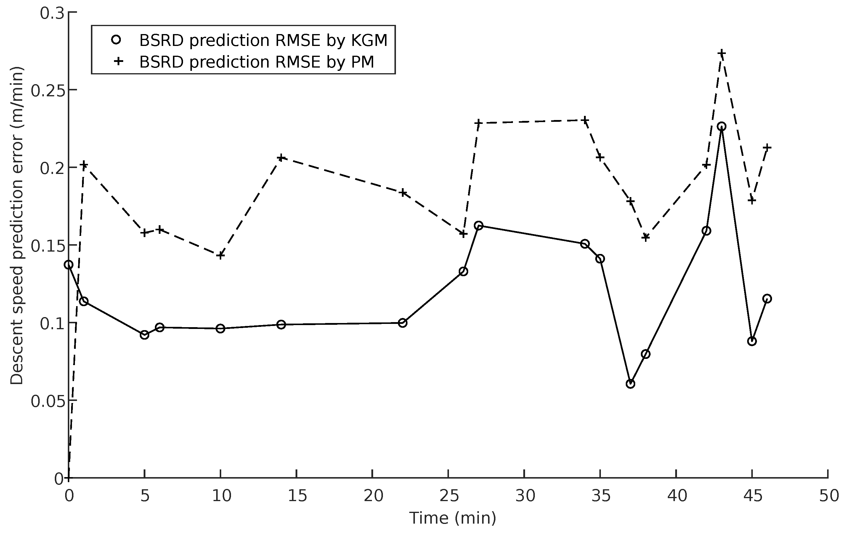
5. Model Performance

We compared the proposed KGM model with the plain data-driven description model (PM), which was adopted in our previous work [3], to examine the difference in their prediction performance.

5.1. Prediction Accuracy

Both the prediction results of the BSRP in Figure 9 and BSRD in Figure 10 correspond to the cases whose EBDFs have been previously presented in Figure 7. The subfigures labeled with the same letter (e.g., (a)) correspond to the same case.

Regarding profile prediction, Figure 9 indicates that both the PM model and the KGM model can provide general predictions for the future BSRP. Maximum absolute error (MAE) and RMSE were adopted to quantify the different accuracies in detail. The results are listed in

Table 2. Summary of quantified prediction accuracy.

Case	Model	BSRP		BSRD
		MAE	RMSE	MAE	RMSE
1	KGM	0.2537	0.1081	0.0561	0.0353
	PM	0.5959	0.2970	0.1429	0.0732
2	KGM	0.5801	0.2913	0.1633	0.0987
	PM	0.8601	0.5823	0.2280	0.1325

. For the case shown in Figure 9a, the shape variation in BSRP from the past to the future is not obvious, and the prediction accuracy of the KGM is slightly higher than that of the PM. However, for the case in Figure 9b, the KGM surpasses PM in terms of providing a higher prediction accuracy. Additionally, this superiority mainly resides in the region $0.5<r<2.5$, where the shape of the BSRP varies significantly.

Regarding BSRD prediction, first, the general prediction results are presented in Figure 10c, in which the axes have equal scaling. Both models can predict the general BSRD shape well. In Figure 10a,b, with a smaller range of the vertical axes, the performance gap between the two models was singularized. As indicated by the quantified comparison results presented in Table 2, the KGM is slightly better than the PM in predicting the BSRD.

A synthetic analysis of the BSRP and BSRD prediction results revealed two characteristics of the KGM model. First, the KGM model stands out in terms of its method for addressing the prediction problems of nonuniform radial distributions of descent speed. Considering its modeling mechanism, the linear combination of Gaussian functions at different radial positions to approximate the EBDF allows the ability to better represent the variability. Second, the prediction accuracy of the BSRD in the KGM model is related to that of the corresponding BSRP. As can be observed, the quantitative results presented in Table 2, compared to the prediction results of Case 1, with the lower prediction accuracy of the BSRP, the prediction accuracy of the BSRD is also lower for Case 2. This outcome originates from the relationship stated in Equation (25): the prediction accuracy of the BSRD can be regarded as a function of the prediction accuracy of the BSRP. Therefore, the former will deteriorate with the latter.

5.2. Prediction Performance Decay

To explore the variation in prediction performance with time, an EBDF was identified from one data segment. Then, it was used with the detection results of the BSRP to predict the BSRD in the subsequent $47min$. The PM model result was also adopted as a reference. Figure 11 demonstrates the variation in the prediction RMSE with time.

Since the PM model adopts a direct data-driven mechanism to calculate the BSRD, its performance in this test can be regarded as a base level. As shown in Figure 11, during 0–$47min$, its prediction accuracy continues to oscillate in a range of 0.15–$0.28\mathrm{m}/\min$. Compared to the PM model, the performance variation in the KGM model can be divided into two stages. During 0–$20min$, the prediction RMSE remains steady at approximately $0.1\mathrm{m}/\min$. Its prediction accuracy is higher and more stable than that of the PM. Thereafter, during 20–$47min$, although there are oscillations in the prediction accuracy, its prediction RMSE remains smaller than that of the PM at every corresponding time.

Here, we have two remarks regarding the above results. First, it is reasonable that the KGM is superior to the PM in the comparison of performance decay. Compared to the PM, the KGM is based on the kinematic flow mechanism and hence has the ability to imitate the behavior of burden solid flow in a subsequent period of time. Second, the phenomenon that the KGM provides a stable prediction performance in the first $20min$ manifests the rationality and validity of Assumption 3: the burden descent speed field remains unchanged during the time of the model prediction.

Finally, limited by the size of the adopted dataset, the results presented above are solely used for previewing the difference in prediction performance resulting from the differences in the modeling mechanism between the PM and the KGM. An in-depth analysis of the prediction performance of the KGM will be performed with a larger dataset in future work.

6. Conclusions

Based on the modeling mechanism of kinematic flow, a model integrated with a data-driven technique for the prediction of the BSRD in the BF was proposed. The data used in this research were from the detection results of a real operating BF, collected using a MSR system. Solving the boundary PDE equation associated with the governing equations of the mechanism of kinematic flow can be formulated as solving an optimization problem in which the measurement output of the BSRD are used as the training data. A proof of the existence and uniqueness of the predicted BSRP is given. Compared with the plain data-driven description model proposed in our previous work, the current model provides higher prediction accuracy, especially when there is obvious variability in the BSRD. Imbedding the purposed model into the prediction model of burden shape after charging, the accuracy of the prediction of the burden layer thicknesses can be further improved.

References

1. Geerdes, M.; Chaigneau, R.; Kurunov, I.; Lingiardi, O.; Ricketts, J. Modern Blast Furnace Ironmaking an Introduction, 3rd ed.; IOS Press: Amsterdam, The Netherlands, 2015. [Google Scholar]
2. Yang, Y.; Yin, Y.; Wunsch, D.; Zhang, S.; Chen, X.; Li, X.; Cheng, S.; Wu, M.; Liu, K.Z. Development of Blast Furnace Burden Distribution Process Modeling and Control. ISIJ Int. 2017, 57, 1350–1363. [Google Scholar] [CrossRef] [Green Version]
3. Tian, J.; Tanaka, A.; Hou, Q.; Chen, X. Radar Detection-Based Modeling in a Blast Furnace: A Prediction Model of Burden Surface Shape After Charging. ISIJ Int. 2018, 58, 1999–2008. [Google Scholar] [CrossRef]
4. Ichida, M.; Takao, M.; Kunitomo, K.; Matsuzaki, S.; Deno, T.; Nishihara, K. Radial Distribution of Burden Descent Velocity Near Burden Surface in Blast Furnace. ISIJ Int. 1996, 36, 493–502. [Google Scholar] [CrossRef]
5. Zhou, P.; Shi, P.Y.; Song, Y.P.; Tang, K.L.; Fu, D.; Zhou, C.Q. Evaluation of Burden Descent Model for Burden Distribution in Blast Furnace. J. Iron Steel Res. Int. 2016, 23, 765–771. [Google Scholar] [CrossRef]
6. Zhang, S.J.; Yu, A.B.; Zulli, P.; Wright, B.; Tuzun, U. Modelling of the Solids Flow in a Blast Furnace. ISIJ Int. 1998, 38, 1311–1319. [Google Scholar] [CrossRef]
7. Zhang, S.; Yu, A.; Zulli, P.; Wright, B.; Austin, P. Numerical Simulation of Solids Flow in a Blast Furnace. Appl. Math. Model. 2002, 26, 141–154. [Google Scholar] [CrossRef]
8. Natsui, S.; Ueda, S.; Fan, Z.; Andersson, N.; Kano, J.; Inoue, R.; Ariyama, T. Characteristics of Solid Flow and Stress Distribution Including Asymmetric Phenomena in Blast Furnace Analyzed By Discrete Element Method. ISIJ Int. 2010, 50, 207–214. [Google Scholar] [CrossRef]
9. Fu, D.; Chen, Y.; Zhou, C.Q. Mathematical Modeling of Blast Furnace Burden Distribution With Non-Uniform Descending Speed. Appl. Math. Model. 2015, 39, 7554–7567. [Google Scholar] [CrossRef]
10. Yang, K.; Choi, S.; Chung, J.; Yagi, J.I. Numerical Modeling of Reaction and Flow Characteristics in a Blast Furnace With Consideration of Layered Burden. ISIJ Int. 2010, 50, 972–980. [Google Scholar] [CrossRef]
11. Takatani, K.; Inada, T.; Ujisawa, Y. Three-Dimensional Dynamic Simulator for Blast Furnace. ISIJ Int. 1999, 39, 15–22. [Google Scholar] [CrossRef]
12. Nedderman, R.; Tuzun, U. A Kinematic Model for the Flow of Granular Materials. Powder Technol. 1979, 22, 243–253. [Google Scholar] [CrossRef]
13. Chen, J.; Akiyama, T.; Nogami, H.; Yagi, J.I.; Takahashi, H. Modeling of Solid Flow in Moving Beds. ISIJ Int. 1993, 33, 664–671. [Google Scholar] [CrossRef]
14. Wu, J.; Chen, J.; Yang, Y. A Modified Kinematic Model for Particle Flow in Moving Beds. Powder Technol. 2008, 181, 74–82. [Google Scholar] [CrossRef]
15. Chen, X.; Wei, J.; Xu, D.; Hou, Q.; Bai, Z. 3-dimension Imaging System of Burden Surface With 6-radars Array in a Blast Furnace. ISIJ Int. 2012, 52, 2048–2054. [Google Scholar] [CrossRef]
16. Wei, J.; Chen, X.; Wang, Z.; Kelly, J.; Zhou, P. 3-dimension Burden Surface Imaging System With T-Shaped Mimo Radar in the Blast Furnace. ISIJ Int. 2015, 55, 592–599. [Google Scholar] [CrossRef]
17. Wei, J.; Ma, J.; Wan, L.; Jia, G.; Chen, X. Measuring System of Radial Burden Surface With Mechanical Swing Radar in a Blast Furnace. Iron Steel 2015, 50, 94–100. [Google Scholar]
18. Mullins, W.W. Stochastic Theory of Particle Flow Under Gravity. J. Appl. Phys. 1972, 43, 665–678. [Google Scholar] [CrossRef]
19. Tuzun, U.; Houlsby, G.; Nedderman, R.; Savage, S. The Flow of Granular Materials—II Velocity Distributions in Slow Flow. Chem. Eng. Sci. 1982, 37, 1691–1709. [Google Scholar] [CrossRef]
20. Cannon, J.R. The One-Dimensional Heat Equation; Number 23 in Encyclopedia of Mathematics and Its Applications; Cambridge University Press: Cambridge, UK, 1984. [Google Scholar]
21. Hsieh, P.F.; Sibuya, Y. Basic Theory of Ordinary Differential Equations; Universitext, Springer: New York, NY, USA, 1999. [Google Scholar]
Figure 1. Radar placement on top of the BF.
Metals 09 00609 g001
Figure 2. Mechanical servo system of radar.
Metals 09 00609 g002
Figure 3. The variation in BSRDs within half an hour: (af) detection results obtained at different time.
Metals 09 00609 g003
Figure 4. Kinematic modeling mechanism diagram.
Metals 09 00609 g004
Figure 5. Flow of the proposed prediction model.
Metals 09 00609 g005
Figure 6. Solution domain of the descent speed along the burden radius.
Metals 09 00609 g006
Figure 7. EBDFs from two data segments. (a) EBDF corresponds to Case 1; (b) EBDF corresponds to Case 2.
Metals 09 00609 g007
Figure 8. The relationship between m and the approximation RMSE.
Metals 09 00609 g008
Figure 9. Comparison of prediction accuracy of BSRP. (a) Results for Case 1; and (b) results for Case 2.
Metals 09 00609 g009
Figure 10. Comparison of BSRD prediction accuracy. (a) Results for Case 1; (b) results for Case 2; and (c) results presented on equal scaled axes. The upper subgraph corresponds to Case 1, and the lower one corresponds to Case 2.
Metals 09 00609 g010
Figure 11. Model comparison of the variation in prediction performance with time.
Metals 09 00609 g011