An Extended Iterative Identification Method for the GISSMO Model

Abstract

This study examines an extended method to obtain the parameters in the Generalized Incremental Stress State Dependent Damage (GISSMO) model. This method is based on an iterative Finite Element Method (FEM) method aiming at predicting the fracture behavior considering softening and failure. A large number of experimental tests have been conducted on four different alloys (7003 aluminum alloy, ADC12 aluminum alloy, ZK60 magnesium alloy and 20CrMnTiH Steel), here considering tests that span a wide range of stress triaxiality. The proposed method is compared with the two existing methods. Results show that the new extended Iterative FEM method gives the good estimate of the fracture behaviors for all four alloys considered.

1. Introduction

The research into lightweight and high-durability materials used in automobiles has greatly increased in recent years, due to an increased focus on preserving natural resources and reducing air pollution. One effective way to achieve weight reduction is through material development, but with this approach comes a demand for accurately predicting the flow and damage behaviors of the new material. [1,2] Flow behavior and damage evolution is, however, a challenging task.

A large amount of research has been focused on evaluating the flow and fracture properties through micromechanics-based consideration [3,4,5,6,7,8,9,10,11]. Among these are the porous plasticity models, the best-known being the classical model by Gurson [3] that includes the growth of voids in a metallic matrix and a yield condition that relates to porosity. The Gurson model and many of its subsequent extensions agree well with experiments; however, it fails to predict the material behavior under shear dominated loading conditions. To remedy this issue, Nahshon and Hutchinson [12] distinguished shear dominated states by the third invariant of stress. Dæhli et al. [13] extended the Gurson model by Lode-dependent void evolution, both successfully predicting fracture under low triaxiality. However, the Gurson model is computationally inefficient as the element size must scale with the dominant void sparking. Thus, the phenomenological fracture models outweigh the porous models in industrial applications, as these models often require fewer material constants to be determined through data fitting. The typical fracture models [14,15,16,17] are formalized on experimental observation, which directly related to the stress state. Identified through the stress, the triaxiality and the lode angle are proposed. Compared to the Gurson model, the Johnson-Cook (JC) model [17,18,19] predicts the fracture locus accounting for the strain, the strain rate and the temperature, and the model parameters in the JC model is easily to calibrate. Other fracture models in Ref. [14,15,20] predicts the fracture locus in 3D space with more accuracy. Moreover, it is worth noticing that these fracture models are uncoupled from flow behavior, which is described by the standard material model. The Generalized Incremental Stress State Dependent Damage (GISSMO) Model which is developed by Neukamm [21,22], fully describes the ductile damage accounting for material softening and fracture. The fracture behavior is described by the damage variable and the damage softening behavior is represented by an instability measure. As the GISSMO model meets the industrial requirements, it finds wide use in crashworthiness and forming process simulations [23,24,25,26,27].

The parameter calibration strongly influences the accuracy of a numerical prediction. The constitutive constants are classically obtained by graphical analysis [28] and linear regression methods [29] to fit experimental data. For example, the force-displacement curves obtained from experimental data is transformed into equivalent stress-strain curves, from which constitutive parameters are obtained [30]. However, these calculation methods are conducted under assumptions of relatively small strain variation, failing to predict fracture behavior in several industrial applications. Recently, an iterative FEM method [31,32,33,34] has been developed for parameter calibration that, based on trial and error, can determine a set of parameters, which leads to good agreements between experimental data and numerical results. Xiao [31] obtained the fracture parameters through the iterative FEM method to predict the fracture locus in the 3D stress state. However, fracture parameters by the iterative FEM method are difficult to predict the fracture behavior considering softening.

In this paper, an extended iterative FEM method is proposed to obtain the GISSMO parameters. The accuracy of the inverse iterative FEM method is then validated by considering four different types of alloy through an extensive experimental program that subject the materials in different stress states. FEM procedures are conducted for three sets of validated parameters obtained by three methods. The accuracy of the three methods is evaluated. These stress-strain curves and fracture modes observed throughout the tests are compared to the model predictions. Finally, a discussion on the iterative FEM method is conducted.

2. Materials and Methods

2.1. Experiment Method

Four kinds of alloy, listing 7003-T6 aluminum (Test # 1–7), ADC12 aluminum (Test # 8–11), ZK60 magnesium (Test # 12–18) and 20CrMnTiH steel (Test # 19–25), are designated as the testing material with the chemical composition shown in

Table 1. Chemical composition of the materials used in the study (wt.%). The single value means the maximum value of element’s concentration.

Materials	Al	C	Cr	Cu	Fe	Mg	Mn	Ni	P	Pb	S	Sn	Si	Ti	Zr	Zn
7003Al	Bal.	-	-	0.1	0.35	0.5–1	0.3	-	-	-	-	-	0.3	0.2	0.05–0.25	5.5–6.5
ADC12	Bal.	-	-	1.5–3.5	1.2	0.3	0.5	0.5	-	0.1	-	0.1	9.6–12.0	-	-	1
ZK60	-	-	-	-	-	Bal.	-	-	-	-	-	-	-	-	0.45–0.9	4.8–6.2
CrMnTiH	-	0.17–0.23	1–1.35	0.3	Bal.	-	0.8–1.15	0.3	0.04	-	0.04	-	0.17–0.37	0.01–0.1	-	-

. These alloys are extensively used in aerospace and automobile industries. Figure 1 presents 25 different specimens for a wide range of stress states. The dimensions of tensile specimen are recommended by the GB/T228.1-2010 standard. All tests are performed in the ETM504C electronic universal testing machine (Suzhou Dymeter Automotive testing technology co., LTD, Suzhou, China) with a load range of (5–50) kN and a speed range of (0.001–500) mm/min. The deforming results are measured by the Digital Image Correlation (DIC) method, and the loading results are measured by force cell. For DIC method, signature is marked in undeformed specimen, and displacement is measured by searching the signature in deformed specimen. The crosshead speed of the testing machine is kept constant at 1.8 mm/min for smooth tensile tests and 0.2 mm/min for notched and shear tests. These tests are performed in the ambient air at the room temperature. Following experimental data is recorded: the stress-strain relation, fracture mode, and elongation.

2.2. Effective Stress and Strain Curves

Experimental obtained engineering curves cannot be directly used in parameter calibration. In small strain, engineering curves is transformed into true stress-strain curves by volume constancy law,

$$\begin{array}{l}{\mathsf{\epsilon }}_{\mathrm{true}}=\ln \left(1+{\mathsf{\epsilon }}_{\mathrm{eng}}\right)\\ {\mathsf{\sigma }}_{\mathrm{true}}={\mathsf{\sigma }}_{\mathrm{eng}}\left(1+{\mathsf{\epsilon }}_{\mathrm{eng}}\right)\end{array}$$

(1)

where ${\mathsf{\sigma }}_{\mathrm{true}}$ and ${\mathsf{\epsilon }}_{\mathrm{true}}$ is true stress and true strain. ${\mathsf{\sigma }}_{\mathrm{eng}}$ and ${\mathsf{\epsilon }}_{\mathrm{eng}}$ is engineering stress and strain. For some metals Equation (1) cannot compensate for the large necking effects, constitutive models are used for extrapolating the after-necking stress-strain curves. Taken smooth tension for example, the engineering curves are transformed into true stress-strain curves by volume constancy law. Then, the soften part in the true stress-strain curve is extrapolated by the power law of Ludwik [35]. The extrapolated curve is shown in Figure 2 as the yellow dash one. The effective stress-strain curve is obtained by subtracting off the elastic strain and inputting the true stress. The effective stress-strain curve is used in material model calibration. The effective strain at fracture point is input as initial value in iterative FEM method.

2.3. GISSMO Model

The GISSMO, developed by Neukamm et al. [21,22] and Basaran et al. [36], ensures flexibility for a wide range of metal as it can correctly predict damage regardless the details of the material model formulation. Besides, the GISSMO targets damage prediction that accounts for material instability, localization, and failure. Damage accumulation, which is illustrated by Johnson [17] and Xue [37], is based on an incremental formulation found from

$$\mathsf{\Delta }D=\frac{n}{{\mathsf{\epsilon }}^f}{D}^{\left(1-\frac{1}{n}\right)}{\dot{\mathsf{\epsilon }}}_p,$$

(2)

This equation considers the nonlinear relation between plastic strain and internal damage [38,39], and the damage exponent n allows for a nonlinear accumulation of damage until failure. The equivalent plastic strain increment is denominated as ${\dot{\mathsf{\epsilon }}}_p$. ${\mathsf{\epsilon }}^f$ represents the equivalent plastic failure strain which allows for an arbitrary definition of triaxiality dependent failure strains ${\mathsf{\epsilon }}^f\left({\mathsf{\sigma }}^{*}\right)$ by inputting a tabulated curve. Triaxiality is defined as $p/{\mathsf{\sigma }}_m$, in which p is the average main stress and ${\mathsf{\sigma }}_m$ is the von Mises stress. D is the damage value, which accumulates in each element during deformation. When D = 1, the element is deleted.

Similar to damage accumulation, material instability is determined as

$$\mathsf{\Delta }F=\frac{n}{{\mathsf{\epsilon }}^c}{F}^{\left(1-\frac{1}{n}\right)}{\dot{\mathsf{\epsilon }}}_p,$$

(3)

where ${\mathsf{\epsilon }}^c$ is the triaxiality dependent critical strain ${\mathsf{\epsilon }}^c\left({\mathsf{\sigma }}^{*}\right)$ which acts as an activation for coupling damage and stress. F is the instability measure. If F = 0, the material is undeformed. F = 1 corresponds to the onset of localization.

As soon as F reaches unity, the element stress is reduced by

$$\mathsf{\sigma }=\tilde{\mathsf{\sigma }}\left[1-{\left(\frac{D-D_{\mathrm{crit}}}{1-D_{\mathrm{crit}}}\right)}^m\right],$$

(4)

where $\mathsf{\sigma }$ is the modified stress and $\tilde{\mathsf{\sigma }}$ is the current stress. D_crit is the damage only comes to some value when F reaches unity. m is a fading exponent intended to better depict the rate of material softening.

2.4. Extended Iterative Finite Element Method

The extended Iterative FEM (EIFEM) method is a trial-and-error method, aiming at obtaining stress and strain at large strain. The EIFEM method is inspired by the method in Ref. [31], which can obtain parameters in the JC model. This paper extended the model to calibrate parameters in the GISSMO model. Five parameters need to be calibrated, including stress triaxiality ${\mathsf{\sigma }}^{*}$, fracture strain ${\mathsf{\epsilon }}^f$, critical strain ${\mathsf{\epsilon }}^c$, fading exponent m, and damage exponent n. The proposed procedure of the extended Iterative FEM method (EIFEM) is,

• Initial value of ${\mathsf{\epsilon }}_0^f$, ${\mathsf{\epsilon }}_0^c$, m₀ and n₀. ${\epsilon }_0^f$ is the fracture strain and ${\mathsf{\epsilon }}_0^c$ is the necking strain at obtained effective stress-strain curve. m₀ and n₀ can be set to arbitrary value. in this paper, m₀ = 1, n₀ = 3.
• Iteration till the shape of numerical force and displacement curve after necking coincide with experimental one. 3D FEM simulation by LS-DYNA is conducted to calculate elongation $\mathsf{\Delta }{L}^{\mathrm{FEM}}$. In simulation, the deforming process is predicted by the JC material model and the fracture model is the GISSMO model. If numerical shape differs experimental shape, n and m are modified by n_i = n_{i – 1} − 1 and m_i = m_{i − 1} + 0.5 till convergence.
• Iteration till the experimental elongation coincides with the numerical elongation $\mathsf{\Delta }{L}^{\mathrm{EXP}}=\mathsf{\Delta }{L}^{\mathrm{FEM}}$. If $\mathsf{\Delta }{L}^{\mathrm{EXP}}\ne \mathsf{\Delta }{L}^{\mathrm{FEM}}$, ${\mathsf{\epsilon }}^f$ would be modified by ${\mathsf{\epsilon }}_{i + 1}^f\times \mathsf{\Delta }{L}^{\mathrm{EXP}}={\mathsf{\epsilon }}_i^f\times \mathsf{\Delta }{L}_i^{\mathrm{FEM}}$. If ${\mathsf{\epsilon }}_i^f={\mathsf{\epsilon }}_i^c$ but $\mathsf{\Delta }{L}^{\mathrm{FEM}}$ still unequal to $\mathsf{\Delta }{L}^{\mathrm{EXP}}$, ${\mathsf{\epsilon }}^c$ is modified by ${\mathsf{\epsilon }}_{i+1}^c\times \mathsf{\Delta }{L}_n^{\mathrm{EXP}}={\mathsf{\epsilon }}_i^c\times \mathsf{\Delta }{L}_{n\left(i\right)}^{\mathrm{FEM}}$. $\mathsf{\Delta }{L}_n$ is the displacement at necking point. A satisfied pair of ${\mathsf{\epsilon }}^c$ and ${\mathsf{\epsilon }}^f$ is obtain when $\mathsf{\Delta }{L}^{\mathrm{EXP}}=\mathsf{\Delta }{L}^{\mathrm{FEM}}$.
• Check if the standard deviation below 3%. The standard deviation (Std) between experimental and numerical curves is defined as

  $$\mathrm{Std}=\frac{{\displaystyle {\int }_0^{l_f}\left|f_{\mathrm{Exp}}(l)-f_{\mathrm{FEM}}(l)\right|dl}}{\mathrm{Max}\left\{f_{\mathrm{Exp}}(l)\right\}{l}_f},$$

  (5)

  where l is displacement. The iteration is continued until the Std below 3%. Otherwise return to Step 2 and renew the number of m, n, ${\mathsf{\epsilon }}^c$ and ${\mathsf{\epsilon }}^f$ till convergence. In the last iterative FEM simulation, ${\mathsf{\sigma }}^{*}$ is obtained at the fracture element right before deleting element.

2.5. Finite Element Method

The finite element (FE) analysis is conducted by the explicit mechanical solver of the commercial finite element code LS-DYNA. FE models for tensile tests are meshed through 8-node hexahedron elements by one-point integration, with single-point-constrain aligned to one side and the prescribed motion to the other side. The average mesh size is 0.2 for each specimen in gauge length. As the FEM mesh are similar between materials, the representative FEM mesh for ZK60 alloy are shown in Figure 3. Tensile specimens all move in constants speeds according to experimental speeds. Due to the strain rate insensitivity, the velocity is set at a relatively larger value compared to experiment to reduce the calculating time. The velocity is set at 10 mm/s in this paper. The plastic flow and damage are considered separately. The GISSMO model describes the fractured and damage behavior. In LS-DYNA, the GISSMO model is embedded in the ADD_EROSION which provides the failure and erosion option. The JC material model describes the flow behavior. The JC material model, which is one of the most widely used empirical models, provides an accurate prediction of the flow behavior considering the effects of stress state and strain rate. As all tests are performed at room temperature, the temperature effect is ignored. The strain rate part is also ignored as all experiments are in quasi-static state. The JC material model [40] is simplified as follows:

$${\mathsf{\sigma }}_e=A+B{\mathsf{\epsilon }}_p{}^c,$$

(6)

where A, B, and c are material constants and ${\mathsf{\sigma }}_e$ is the flow stress. By achieving the good fit of smooth tensile experimental data, four parameter sets are calibrated and listed in

Table 3. Parameters for numerical simulation.

Mat.	E/GPa	A	B	c	n	m
7003-T6	66	348	252	0.44	3	2.5
ADC12	33	115	1938	0.67	2	10
ZK60	31	221	316	0.43	2	1.5
20CrMnTiH	125	944	754	0.28	3	3.5

. Please note that the elastic modulus is obtained from the elastic region ranging from start point to yielding point (the value stress value is A). This elastic modulus would make the numerical predicted results more accurate.

Fracture curves ${\mathsf{\epsilon }}^f \left({\mathsf{\sigma }}^{*}\right)$, critical strain curves ${\mathsf{\epsilon }}^c \left({\mathsf{\sigma }}^{*}\right)$, the fading exponent m and the damage exponent n are identified through the numerical simulation. Although different GISSMO parameters combinations may lead to a similar numerical result, the effect could be minimized by increasing the number of tests for GISSMO model calibration. Recall the method in Section 2.4, the parameters m and n can be calibrated. The fading exponent m and the damage exponent n are listed in Table 3. ${\mathsf{\epsilon }}^f \left({\mathsf{\sigma }}^{*}\right)$ and ${\mathsf{\epsilon }}^c \left({\mathsf{\sigma }}^{*}\right)$ are cubic spline interpolations of fracture strain and critical strain.

3. Results and Discussion

3.1. Experimental Results

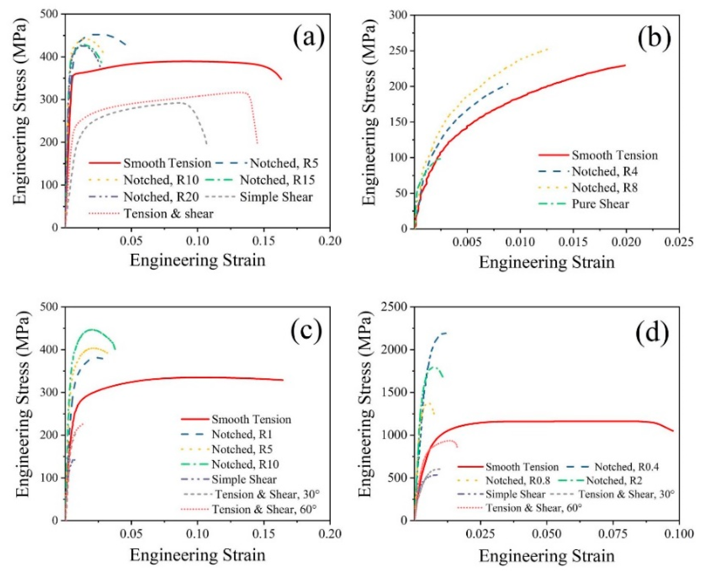
The original experimental results are presented in Figure 4. The engineering stress is calculated by load, which is directly obtained by force cell. The engineering strain is obtained by DIC method. Recall the method in Section 2.2, the effective stress and strain curves are obtained. Then, the triaxiality ${\mathsf{\sigma }}^{*}$, critical strain ${\mathsf{\epsilon }}^c$ and fracture strain ${\mathsf{\epsilon }}^f$ are obtained based on the EIFEM method in Section 2.4. Then ${\mathsf{\sigma }}^{*}$, ${\mathsf{\epsilon }}^c$ and ${\mathsf{\epsilon }}^f$ is used in numerical simulation.

3.2. Numerical Results and Validation

Table 4. Summary of experimental and numerical results.

Mat.	No.	Description	${\mathsf{\sigma }}^{*}$	${\mathsf{\epsilon }}^{\mathit{c}}$	${\mathsf{\epsilon }}^{\mathit{f}}$	Elongation/mm
						Exp.	Num.	R.E. (%) 1
7003-T6	1	Smooth tensile	0.33	0.3	0.79	8.16	8.30	1.80
	2	Pure Shear	−0.01	0.3	0.83	1.94	1.84	4.87
	3	Tensile Shear, 45°	−0.08	0.05	0.73	2.55	2.49	2.33
	4	Notched, R5	0.55	0.02	0.47	0.96	0.97	0.72
	5	Notched, R10	0.46	0.1	0.44	1.19	1.17	1.32
	6	Notched, R15	0.4	0.01	0.50	1.32	1.32	0.24
	7	Notched, R20	0.38	0.01	0.50	1.42	1.45	2.12
ADC12	8	Smooth Tensile	0.34	0.005	0.019	0.70	0.69	1.50
	9	Notched, R4	0.36	0.005	0.033	0.12	0.13	3.52
	10	Notched, R8	0.35	0.005	0.035	0.23	0.23	2.50
	11	Pure shear, flat	−0.03	0.005	0.025	0.10	0.10	1.52
ZK60	12	Smooth Tensile	0.33	0.08	0.697	4.11	4.07	0.84
	13	Notched, R1	0.41	0.10	0.262	0.36	0.35	1.51
	14	Notched, R5	0.46	0.05	0.107	0.65	0.65	0.28
	15	Notched, R10	0.48	0.03	0.289	1.13	1.09	3.39
	16	Pure Shear	0.07	0.26	0.343	0.27	0.27	0.77
	17	Tensile Shear, 30°	0.22	0.05	0.420	0.17	0.17	1.50
	18	Tensile Shear, 60°	0.30	0.09	0.587	0.31	0.31	1.10
20CrMnTiH	19	Round smooth tensile	0.33	0.03	0.17	1.95	1.94	0.51
	20	Round notch, R0.4	0.50	0.03	0.08	0.13	0.13	4.83
	21	Round notch, R0.8	0.64	0.05	0.15	0.08	0.08	1.15
	22	Round notch, R2	0.69	0.03	0.09	0.13	0.12	4.78
	23	Pure shear	−0.07	0.1	0.45	0.34	0.34	0.41
	24	Tensile shear, 30°	0.2	0.1	0.42	0.21	0.22	2.57
	25	Tensile shear, 60°	0.27	0.1	0.34	0.34	0.33	2.08

¹ R.E. denotes the relative error.

presents the experimental and numerical elongation. The relative errors are below 5% for all tests. Figure 5 shows the force and displacement curves for experiment and simulation. Figure 5a presents curves for tensile tests. Numerical results agree with the experimental results well. For 20CrMnTiH steel and 7003 aluminum alloy, the after-necking region in numerical force and displacement curves coincides with the experimental curves. The good agreements are also observed in notched and shear tests shown in Figure 5b–e.

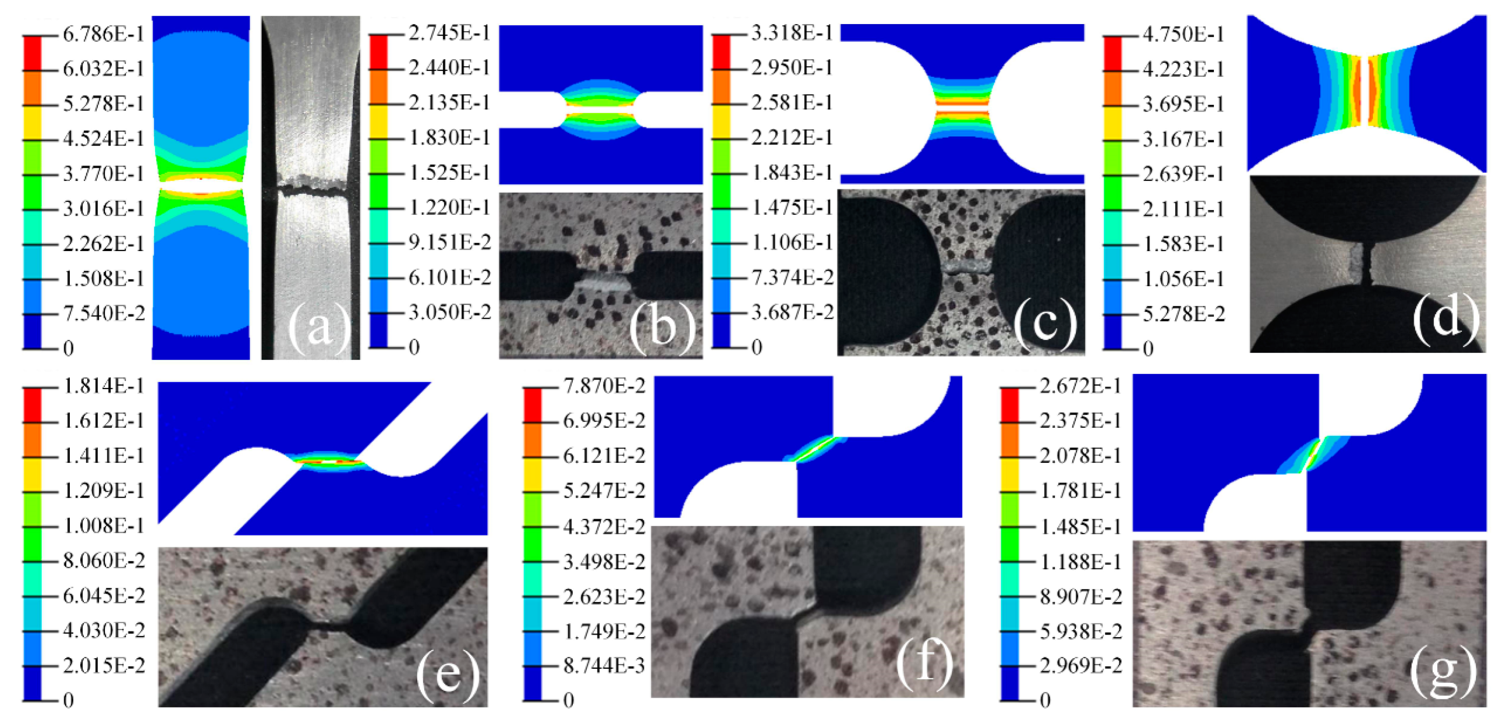
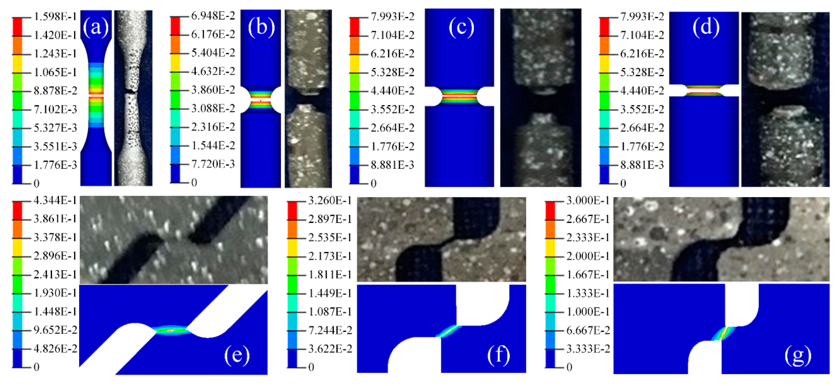
Visual comparisons between experimental and numerical predicted fracture modes are shown in Figure 6, Figure 7, Figure 8 and Figure 9. Good agreements on the fracture modes are observed in those figures, indicating that the EIFEM method can reproduce the fracture behavior for different metals over a wide stress triaxiality with certain accuracy.

3.3. Comparison

To further study the application range of the proposed method, the numerical results predicted by the GISSMO model are compared with other two methods. The first method is widely used in industry for rough calculation. To get the fracture strain in the first method, the experimental obtained force and displacement curves are transposed into effective stress and strain based on method in Section 2.2. Then the fracture strain is obtained at the end point in the effective stress and strain curve. Usually this fracture strain is smaller than the EIFEM obtained fracture strain. To verify which fracture strain is more accurate, the numerical simulation for first method also carried out in LS-DYNA. For better clarification, the notation in first method adds A, so the fracture strain is written as ${\mathsf{\epsilon }}_{\mathrm{A}}^f$. The second method is a commonly used iterative FEM method as in Ref. [31]. Different value of fracture strain can be obtained by this method, and the corresponding notation adds a B, so ${\mathsf{\epsilon }}_{\mathrm{B}}^f$. The stepwise procedure for the second method is shown in Appendix A. The numerical simulation for validating the second method is also conducted.

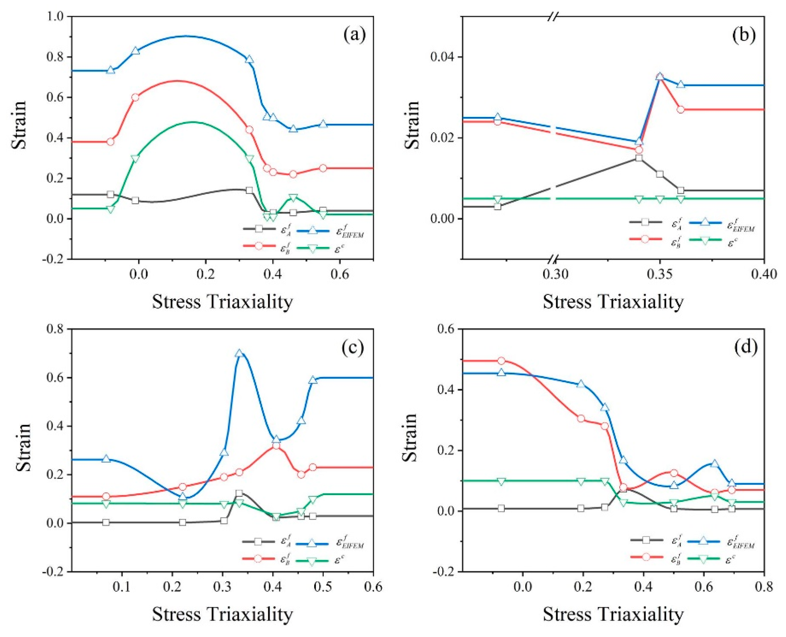
Numerical simulations for the aforementioned two methods carry out in LS-DYNA. The material model is John-Cook model and the fracture model is the GISSMO model, both are consistent with the EIFEM method. The method A and the method B cannot obtain the critical strain ${\mathsf{\epsilon }}^c$, the ${\mathsf{\epsilon }}^c$ in the two method are set to a relatively large constant. Then the GISSMO model cannot display the soften region. The value of ${\mathsf{\epsilon }}^c$ influence the value of ${\mathsf{\epsilon }}^f$. In this paper, the ${\mathsf{\epsilon }}^c$ is set to 1 in method A and method B. m and n are set according to Table 3. The fracture strain vs. stress triaxiality for the three methods are shown in Figure 10.

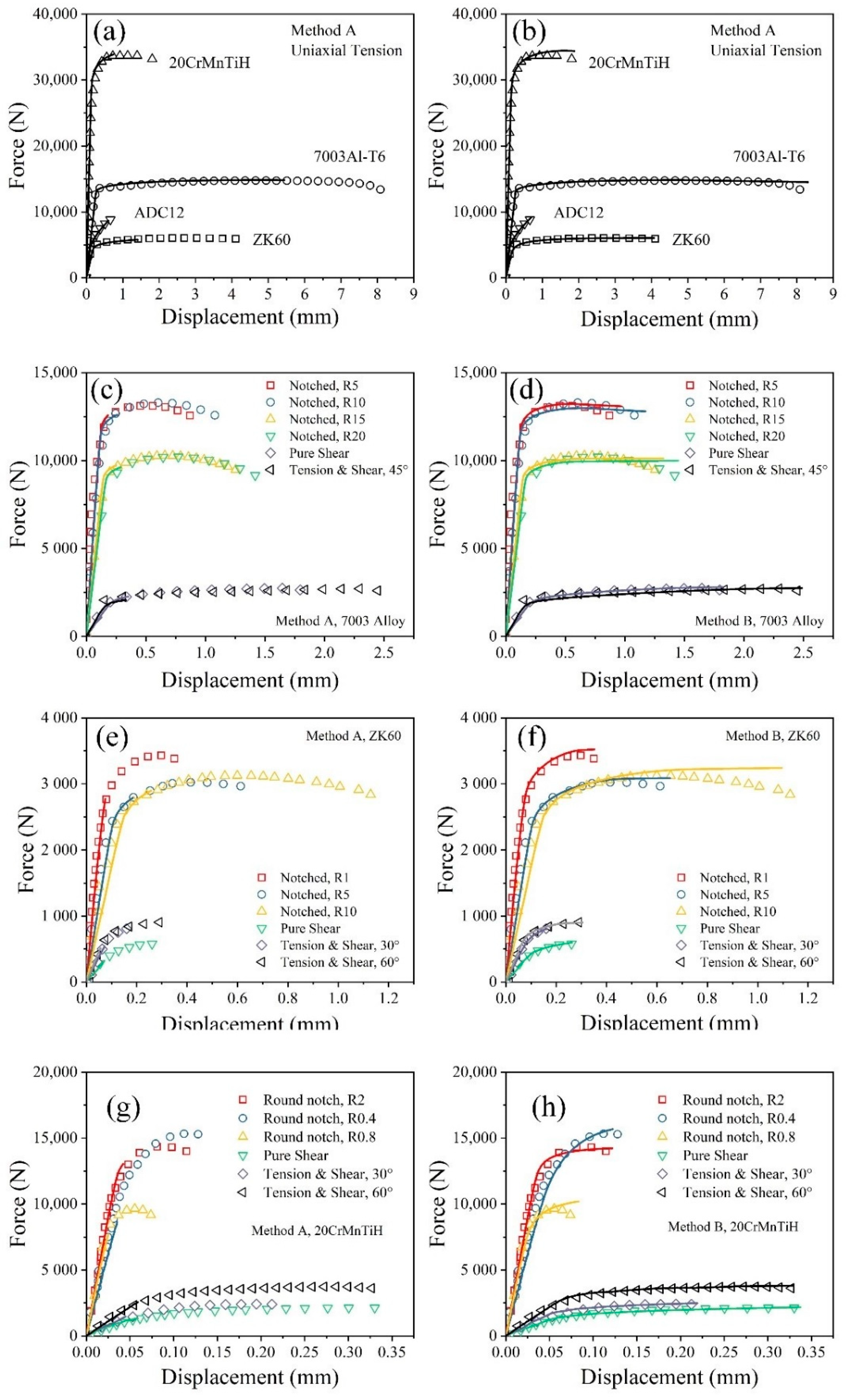
Force and displacement relationships for method A and B is presented in Figure 11. The elongation is discussed firstly. Elongation calculated by method A is much smaller than experimental elongation. Elongations calculated by method B are closer to the experimental data. However, the relative errors for Test No. 9, 10, 17, 20 and 22 (numbered in

Table 2. Summary of experiments.

Mat.	No.	Description	Gauge Length/mm
7003-T6	1	Smooth tensile	50
	2	Pure Shear	19
	3	Tensile Shear, 45°, $\mathsf{\theta }$ = 45°	17.5
	4	Notched, R5, R = 5 mm, H = 10 mm	20
	5	Notched, R10, R = 10 mm, H = 10 mm	20
	6	Notched, R15, R = 15 mm, H = 8 mm	40
	7	Notched, R20, R = 20 mm, H = 8 mm	50
ADC12	8	Smooth Tensile	35
	9	Notched, R4, R = 4mm, H = 5mm	14
	10	Notched, R8, R = 8mm, H = 5mm	18
	11	Pure shear, flat	40.6
ZK60	12	Smooth Tensile	25
	13	Notched, R1	12
	14	Notched, R5	20
	15	Notched, R10	30
	16	Pure Shear	38
	17	Tensile Shear, 30°, $\mathsf{\theta }$ = 30°	21
	18	Tensile Shear, 60°, $\mathsf{\theta }$ = 60°	21
20CrMnTiH	19	Round smooth tensile	20
	20	Round notch, R0.4, R = 0.4 mm, H = 9.2 mm	10.4
	21	Round notch, R0.8, R = 0.8 mm, H = 8.4 mm	10.8
	22	Round notch, R2, R = 2 mm, H = 6 mm	12
	23	Pure shear	38
	24	Tensile shear, 30°, $\mathsf{\theta }$ = 30°	21
	25	Tensile shear, 60°, $\mathsf{\theta }$ = 60°	21

) are beyond 5%, indicating the method B cannot accurately predict the failure behavior. Then the force and displacement curves are compared. For method A, the numerical force and displacement curves overlap the elastic region, failing to predict the harden and soften region. For method B, numerical force and displacement curves in Test No. 2, 3, 8–11,16–18, 23–25 match the experimental data. However, for other tests, the numerical curves cannot capture the soften region. The experiments well predicted by methods B include tests of ADC12 alloy and all shear tests. The experiments failing to be predicted by method B include the uniaxial tensile tests for 7003 alloy and 20CrMnTiH steel and notched tests for 7003 alloy, ADC12 alloy, and 20CrMnTiH steel. The well predicted experiments are brittle fracture (ADC12 alloy) and shear fracture, with relatively small strain and no soften effects. The bad estimated force and displacement curves are featured by obvious soften effects. So, the method B cannot predict soften effect. The reason lies in the constant value of critical strain ${\mathsf{\epsilon }}^c$. ${\mathsf{\epsilon }}^c$ will influence the value of fracture strain ${\mathsf{\epsilon }}^f$. Usually, ${\mathsf{\epsilon }}^f$ in condition ${\mathsf{\epsilon }}^c< {\mathsf{\epsilon }}^f$ is larger than condition ${\mathsf{\epsilon }}^c\ge {\mathsf{\epsilon }}^f$. So, the ${\epsilon }^f$ obtain by the EIFEM method is larger than ${\mathsf{\epsilon }}^f$ by method B. Physically, the soften effect leads to the inaccurate estimate of fracture stain. Usually, ${\mathsf{\epsilon }}_{\mathrm{EIFEM}}^f\ge {\mathsf{\epsilon }}_B^f\ge {\mathsf{\epsilon }}_A^f$. In conclusion, method A is not recommending unless for small strain conditions or very rough calculation. Method B can be safely used in deformation with little or no soften effects. The EIFEM method can accurately predict the large deformation and obvious soften conditions.

4. Conclusions

This paper validates the accuracy for an extended parameter identification method by experiments and simulations, followed by comparison with two existing methods. The EIFEM method obtains the parameters in the GISSMO fracture model. The numerical obtained elongation, force, and displacement curves and the fractured position agree well with experiment. The EIFEM method achieves the best estimate compared with other two methods. Method A is recommended to use in small strain conditions or rough calculation. Method B can be used in metal with little or no soften effects. The EIFEM method can be used in predicting the large deformation and obvious soften effects.

References

- Hu, M.Q.; Zhang, J.J.; Sun, B.Z.; Gu, B.H. Finite element modeling of multiple transverse impact damage behaviors of 3-D braided composite beams at microstructure level. Int. J. Mech. Sci. 2018, 148, 730–744. [Google Scholar] [CrossRef]
- Spagnoli, A.; Terzano, M.; Brighenti, R.; Artoni, F.; Stahle, P. The fracture mechanics in cutting: A comparative study on hard and soft polymeric materials. Int. J. Mech. Sci. 2018, 148, 554–564. [Google Scholar] [CrossRef]
- Gurson, A.L. Continuum theory of ductile rupture by void nucleation and growth: Part I Yield criteria and flow rules for porous ductile media. J. Eng. Mater-T ASME 1977, 99, 2–15. [Google Scholar] [CrossRef]
- McClintock, F.A. A criterion for ductile fracture by the growth of holes. Int. J. Appl. Mech. 1968, 35, 363–371. [Google Scholar] [CrossRef]
- Nguyen, N.T.; Kim, D.Y.; Kim, H.Y. A continuous damage fracture model to predict formability of sheet metal. Fatigue Fract. Eng. Mater. Struct. 2013, 36, 202–216. [Google Scholar] [CrossRef]
- Nielsen, K.L.; Tvergaard, V. Ductile shear failure or plug failure of spot welds modelled by modified Gurson model. Eng. Fract. Mech. 2010, 77, 1031–1047. [Google Scholar] [CrossRef]
- Rice, J.R.; Tracey, D.M. On the ductile enlargement of voids in triaxial stress fields. J. Mech. Phys. Solids 1969, 17, 201–217. [Google Scholar] [CrossRef]
- Tvergaard, V.; Needleman, A. Analysis of the cup-cone fracture in a round tensile bar. Acta Metall. 1984, 32, 157–169. [Google Scholar] [CrossRef]
- Xue, L. Constitutive modeling of void shearing effect in ductile fracture of porous materials. Eng. Fract. Mech. 2008, 75, 3343–3366. [Google Scholar] [CrossRef]
- Cricrì, G. A consistent use of the Gurson-Tvergaard-Needleman damage model for the R-curve calculation. Fract. Struct. Integrity 2013, 7, 161–174. [Google Scholar] [CrossRef]
- Sepe, R.; Lamanna, G.; Caputo, F. A robust approach for the determination of Gurson model parameters. Fract. Struct. Integrity 2016, 10, 369–381. [Google Scholar] [CrossRef]
- Nahshon, K.; Hutchinson, J.W. Modification of the Gurson model for shear failure. Eur. J. Mech. A Solids 2008, 27, 1–17. [Google Scholar] [CrossRef]
- Dæhli, L.E.; Morin, D.; Børvik, T.; Hopperstad, O.S. A Lode-dependent Gurson model motivated by unit cell analyses. Eng. Fract. Mech. 2018, 190, 299–318. [Google Scholar] [CrossRef]
- Bao, Y.; Wierzbicki, T. On fracture locus in the equivalent strain and stress triaxiality space. Int. J. Mech. Sci. 2004, 46, 81–98. [Google Scholar] [CrossRef]
- Bao, Y.; Wierzbicki, T. A comparative study on various ductile crack formation criteria. J. Eng. Mater-T ASME 2004, 126, 314–324. [Google Scholar] [CrossRef]
- Bao, Y.; Wierzbicki, T. On the cut-off value of negative triaxiality for fracture. Eng. Fract. Mech. 2005, 72, 1049–1069. [Google Scholar] [CrossRef]
- Johnson, G.R.; Cook, W.H. Fracture characteristics of three metals subjected to various strains, strain rates, temperatures and pressures. Eng. Fract. Mech. 1985, 21, 31–48. [Google Scholar] [CrossRef]
- Senthil, K.; Iqbal, M.A. Effect of projectile diameter on ballistic resistance and failure mechanism of single and layered aluminum plates. Theor. Appl. Fract. Mech. 2013, 67–68, 53–64. [Google Scholar] [CrossRef]
- Xue, L.; Ling, X.; Yang, S.S. Mechanical behaviour and strain rate sensitivity analysis of TA2 by the small punch test. Theor. Appl. Fract. Mech. 2019, 99, 9–17. [Google Scholar] [CrossRef]
- Benzerga, A.A.; Surovik, D.A.; Keralavarma, S.M. On the path-dependence of the fracture locus in ductile materials–analysis. Int. J. Plasticity 2012, 37, 157–170. [Google Scholar] [CrossRef]
- Neukamm, F.; Feucht, M.; Haufe, A. Considering damage history in crashworthiness simulations. In Proceedings of the 7th European LS-DYNA Conference, Salzburg, Austria, 14–15 May 2009. [Google Scholar]
- Neukamm, F.; Feucht, M.; Haufe, A.; Roll, K. On closing the constitutive gap between forming and crash simulation. In Proceedings of the 10th Internation LS-DYNA Users Conference, Dearborn, MI, USA, 8–10 June 2008. [Google Scholar]
- Anderson, D.; Butcher, C.; Pathak, N.; Worswick, M.J. Failure parameter identification and validation for a dual-phase 780 steel sheet. Int. J. Solids. Struct. 2017, 124, 89–107. [Google Scholar] [CrossRef]
- Andrade, F.X.C.; Feucht, M.; Haufe, A.; Neukamm, F. An incremental stress state dependent damage model for ductile failure prediction. Int. J. Fract. 2016, 200, 127–150. [Google Scholar] [CrossRef]
- Effelsberg, J.; Haufe, A.; Feucht, M.; Neukamm, F.; Du Bois, P. On parameter identification for the GISSMO damage model. In Proceedings of the 12th International LS-DYNA® Users Conference, Dearborn, MI, USA, 3–5 June 2012. [Google Scholar]
- Haufe, A.; Feucht, M.; Neukamm, F. The Challenge to Predict Material Failure in Crashworthiness Applications: Simulation of Producibility to Serviceability. In Predictive Modeling of Dynamic Processes: A Tribute to Professor Klaus Thoma; Hiermaier, S., Ed.; Springer: Boston, MA, USA, 2009. [Google Scholar]
- Heibel, S.; Nester, W.; Clausmeyer, T.; Tekkaya, A.E. Influence of different yield loci on failure prediction with damage models. In 36th Iddrg Conference—Materials Modelling and Testing for Sheet Metal Forming; Volk, W., Ed.; IOP Publishing: Munich, Germany, 2017; Volume 896. [Google Scholar]
- Cingara, A.M.; McQueen, H.J. New formula for calculating flow curves from high temperature constitutive data for 300 austenitic steels. J. Mater. Process. Technol. 1992, 36, 31–42. [Google Scholar] [CrossRef]
- Khoddam, S.; Lam, Y.C.; Thomson, P.F. The effect of specimen geometry on the accuracy of the constitutive equation derived from the hot torsion test. Steel Res. 1995, 66, 45–49. [Google Scholar] [CrossRef]
- Hu, Y.; Xiao, Y.; Jin, X.; Zheng, H.; Zhou, Y.; Shao, J. Experiments and FEM simulations of fracture behaviors for ADC12 aluminum alloy under impact load. WITH Mater. Int. 2016, 22, 1015–1025. [Google Scholar] [CrossRef]
- Xiao, Y.; Tang, Q.; Hu, Y.; Peng, J.; Luo, W. Flow and fracture study for ZK60 alloy at dynamic strain rates and different loading states. Mater. Sci. Eng. A Struct 2018, 724, 208–219. [Google Scholar] [CrossRef]
- Gavrus, A.; Massoni, E.; Chenot, J.L. An inverse analysis using a finite element model for identification of rheological parameters. J. Mater. Process. Technol. 1996, 60, 447–454. [Google Scholar] [CrossRef]
- Gelin, J.C.; Ghouati, O. An inverse method for determining viscoplastic properties of aluminium alloys. J. Mater. Process. Technol. 1994, 45, 435–440. [Google Scholar] [CrossRef]
- Maniatty, A.; Zabaras, N. Method for solving inverse elastoviscoplastic problems. J. Eng. Mech. 1989, 115, 2216–2231. [Google Scholar] [CrossRef]
- Ludwik, P. Elemente der technologischen Mechanik; Springer: Berlin, Germany, 2013. [Google Scholar]
- Basaran, M.; Wölkerling, S.D.; Feucht, M.; Neukamm, F.; Weichert, D.; AG, D. An extension of the GISSMO damage model based on lode angle dependence. In Proceedings of the LS-DYNA Anwenderforum, Bamberg, Germany, 30 September–1 October 2010. [Google Scholar]
- Xue, L. Ductile fracture modeling: theory, experimental investigation and numerical verification. Ph.D. Thesis, Massachusetts Institute of Technology, Cambridge, UK, 2007. [Google Scholar]
- Tasan, C.C. Micro-mechanical characterization of ductile damage in sheet metal. Ph.D. Thesis, Eindhoven University of Technology, Eindhoven, The Netherlands, 2010. [Google Scholar]
- Weck, A.G. The role of coalescence on ductile fracture. Ph.D. Thesis, McMaster University, Hamilton, ON, Canada, 2007. [Google Scholar]
- Johnson, G.R. A Constitutive Model and Data for Metals Subjected to Large Strains, High Strain Rates and High Temperatures. In Proceedings of the International Symposium on Ballistics, Hague, The Netherlands, 19–21 April 1983; pp. 541–548. [Google Scholar]
Figure 1.
Schematic sketch of the specimen. specified value of R, H and can be found in Table 2. All dimensions are in mm.
Figure 2.
Stress-strain curves for experimental data processing. The red solid curve is the engineering stress-strain curves. The blue solid curve is transformed through the red one by plastic incompressibility condition. To compensate for the non-uniform deformation beyond necking, the blue solid curve is extrapolated by the power law of Ludwik. Yellow dash curve represents modified curve which could be used in calibrating constitutive model.
Figure 3.
The representative FEM model for ZK60 alloy, (a) smooth tensile test, (b) pure shear test, (c) notched tensile test and (d) tensile and notched tests.
Figure 4.
Engineering stress and strain curves for (a) 7003 aluminum alloy, (b) ADC12 aluminum alloy, (c) ZK60 magnesium alloy and (d) 20CrMnTiH Steel.
Figure 5.
Numerical and experimental force and displacement curves. (a) Tensile tests, (b) notched and shear tests for 7003 aluminum alloy, (c) notched and shear tests for ADC12 aluminum alloy, (d) notched and shear tests for ZK60 magnesium alloy and (e) notched and shear tests for 20CrMnTiH steel. Scatters represent experimental data and solid lines represent numerical results hereinafter.
Figure 6.
Fracture mode for 7003Al-T6 aluminum alloy for (a) smooth tensile test, (b) pure shear test, (c) tensile and shear test, (d) notched test for notched radii 5 mm, (e) notched test for notched radii 10 mm, (f) notched test for notched radii 15 mm and (g) notched test for notched radii 20 mm. Hereinafter, the numerical fracture mode is in plastic strain contour.
Figure 7.
Fracture mode for ADC12 aluminum alloy for (a) smooth tensile test, (b) notched test for notched radii 4 mm, (c) notched test for notched radii 8 mm and (d) pure shear test.
Figure 8.
Fracture mode for ZK60 magnesium alloy for (a) smooth tensile test, (b) notched test for notched radii 1mm, (c) notched test for notched radii 5mm, (d) notched test for notched radii 10mm, (e) pure shear test, (f) shear and tensile test at shear angle 30° and (g) shear and tensile test at shear angle 60°.
Figure 9.
Fracture mode for 20CrMnTiH steel for (a) smooth tensile test, (b) notched test for notched radii 2 mm, (c) notched test for notched radii 0.8 mm, (d) notched test for notched radii 0.4 mm, (e) pure shear test, (f) shear and tensile test at shear angle 30° and (g) shear and tensile test at shear angle 60°.
Figure 10.
Strain and triaxiality curves for (a) 7003 aluminum alloy, (b) ADC12 aluminum alloy, (c) ZK60 magnesium alloy and (d) 20CrMnTiH steel.
Figure 11.
Force and displacement curves for (a) uniaxial tensile tests based on method A, (b) uniaxial tensile tests based on method B, (c) 7003Al alloy based on method A, (d) 7003Al alloy based on method B, (e) ZK60 Mg alloy based on method A, (f) ZK60 Mg alloy based on method B, (g) 20CrMnTiH based on method A and (h) 20CrMnTiH based on method B.