Aluminum Alloy Sheet-Forming Limit Curve Prediction Based on Original Measured Stress–Strain Data and Its Application in Stretch-Forming Process

Abstract

A new method, by directly utilizing original measured data (OMD) of the stress–strain relation in the Marciniak–Kuczynski (M–K) model, was proposed to predict the forming limit curve (FLC) of an aluminum alloy sheet. In the groove zone of the M–K model, by establishing the relations of the equivalent strain increment, the ratio of shear stress to the first principle stress and the ratio of the second principle stress to the first principle stress, the iterative formula was established and solved. The equations of theoretical forming limits were derived in detail by using the OMD of the stress–strain relation. The stretching specimens of aluminum alloy 6016-T4 were tested and the true stress–strain curve of the material was obtained. Based on the numerical simulations of punch-stretch tests, the optimized specimens’ shape and test scheme were determined, and the tests for FLC were carried out. The FLC predicted by the proposed method was more consistent with the experimental results of FLC by comparing the theoretical FLCs based on OMD of the stress–strain relation and of that based on traditional power function. In addition, the influences of anisotropic parameter and groove angle on FLCs were analyzed. Finally, the FLC calculated by the proposed method was applied to analyze sheet formability in the stretch-forming process, and the predicted results of FLC were verified by numerical simulations and experiments. The fracture tendency of the formed parts can be visualized in the forming limit diagram (FLD), which has certain guiding significance for fracture judgment in the sheet-forming process.

1. Introduction

Plastic forming of sheet metal keeps an important role in modern industrial production and is widely applied to the aerospace industry, automobile manufacturing, equipment manufacturing, and other fields [1,2,3,4]. Mechanical properties and plastic-forming abilities of alloy sheet were studied [5,6,7], and structural and textural evolutions in plastic forming were analyzed by the view of microstructure [8,9]. The forming limit is an important performance index and process parameter in sheet metal forming [10,11]. In the sheet formability evaluation method, the forming limit curve (FLC) is the most intuitive and widely used [12]. Therefore, predicting FLC accurately and effectively is worthy of further study and test [13].

To predict the FLC precisely, various related theoretical models have been developed. These theoretical models include Swift’s theory of dispersion instability [14], Hill’s concentrated instability theory [15], and Marciniak–Kuczynski’s (M–K) theory based on thickness inhomogeneity assumptions, as well as the Storen–Rice theory [16] and the modified maximum force criterion (MMFC) theory [17,18]. At present, the most widely used is the theoretical model proposed by Marciniak and Kuczynski [19], in which an initial geometrical imperfection is assumed to trigger the occurrence of the localized necking. The M–K theory can combine different stress–strain relations and yield functions to calculate the ultimate strains of the sheet metal, and a great deal of research on the FLC by rationally combining stress–strain relation and yield function has been done [20,21,22]. To select the optimal combination of stress–strain relations and yield criteria, Butuc [20] et al. combined the Swift equation and the Voce equation with the four yield criteria (von Mises, Hill 1948, Hill 1979, and Barlat Yld96) to predict the FLC of the AA6016-T4, and the successful correlation was observed between the experimental FLCs and the calculated limit strains when Yld96 yield criterion and the hardening law of Voce equation were adopted. Yang [21] et al. applied the ductile fracture criterion with the traditional M–K model to study the FLC of AA7075-O aluminum alloy sheet, and a modified M–K model was proposed. Wang [22] et al. combined the Swift equation, the modified Voce equation, and the modified Hockett equation with four yield criteria to analyze the effects of different constitutive equations and yield criteria on the FLCs. Then, the optimal FLCs were obtained by selecting the suitable constitutive equation and yield criterion.

The stress–strain relation of materials is a key factor to accurately predict FLC. In previous studies, the stress–strain curves and the dislocation microstructures were predicted for a wide range of temperatures and strain rates and the prediction agreed quite well with the experimental data [23,24,25]. The experimental stress–strain curves can be explained by employing a small set of physics-based parameters, and the statistical-thermodynamic dislocation is used to analyze the experimental observations of adiabatic shear banding in steel [24]. However, the traditional power approximations were generally used to reflect the stress–strain relation when predicting FLC in the M–K model. Du [26] et al. introduced the power approximations into the M–K model. The theoretical FLC was predicted, and theoretically predicted results of forming limits agreed well with the experimental data. Hou [27] et al. used the curve-fitting method to calculate the strain hardening exponent n and hardening exponent m of Al5083-O aluminum alloy sheet and predicted the FLC of the material. Nader [28] used a modified power exponential hardening model to describe the hardening behavior of aluminum alloy sheets in warm forming, but the theoretical FLCs were not verified by experiments. Barata Da Rocha [29] carried on the FLC prediction of anisotropic sheets by power approximations, and found that the initial groove angle had a significant effect on the forming limits under different strain paths. Li [30] et al. predicted the FLC of the Ti-6Al-4V alloy sheet under the positive-strain path, however, lacking the prediction of the FLC under the negative-strain path. Chu [31] et al. proposed the method based on quadratic polynomial describing the true stress–strain curve, and the theoretical FLCs based on the constitutive model of second order function was significantly more accurate than that based on power approximations. The ductile fracture behavior of the anisotropic 7050-T7451 aluminum alloy plate was investigated, and a novel damage model was proposed to predict the fracture behavior of anisotropic materials [32]. In addition, the theoretical forming limit diagram (FLD) of Al 6061-T6 was acquired and evaluated in an electrohydraulic forming process [33]. The physical model and numerical simulation of a deep drawing process for a box-shaped product were developed, and the best combination of yield locus and hardening law was determined [34].

The methodologies for FLD determination have focused on the FLD with different shapes of the deformed pieces [35]. The widely used method was the Nakazima test, and the different strip-shaped specimens can achieve different strain paths during the test and the complete FLD can be obtained [36]. Marciniak proposed the method that used two elliptical punches and one round punch to determine the right-hand side of the FLD [37]. In this paper, based on the numerical simulations results for specimens with different shapes and sizes, the specimens in different strain paths were tested and the entire FLD was obtained.

The stretch-forming process has been applied to manufacture aerospace, high-speed train, and modern architecture, et al. [38,39,40]. The sheet metal was clamped by a pair of integral rigid clamps in the conventional stretch-forming process, and the large tensile load was usually adopted in order to achieve the complete fit between the sheet metal and the die, so the sheet metal was easily cracked [41]. In order to improve the forming quality, the integral clamps in a conventional stretch-forming process were replaced by discrete clamps in a stretch-forming process based on loading at multi-positions. Cai et al. proposed a new design method for a stretch-forming process based on a minimum deformation path, and which can achieve the manufacture of specified shape parts and the faultless product of large curvature [42]. In order to explore the optimal moving locus of discrete clamps, a series of numerical simulations and experiments were carried out by Yang et al. [43], and the results demonstrated that the strains and stresses of deformed parts presented different distributions when different loading trajectories were adopted. In this paper, the FLC was used to analyze the stretch-forming process of sheet metal, therefore, the related tensile test for stress–strain curve and the punch-stretch experiment for FLC were carried out under the temperature and strain rate similar to those of the stretch-forming process. The new method for FLC prediction directly uses original measured data (OMD) of the stress–strain relation to replace power approximations obtained by fitting the stress–strain data. In addition, the OMD of the stress–strain relation under room temperature was more realistic in the analysis on sheet formability in the stretch-forming process, because the stretch-forming process was generally performed under room temperature and the OMD of the stress–strain relation can strictly indicate the true stress–strain relation of the material. The forming limits by the proposed method were calculated by the detailed theoretical equations. By comparing the theoretical FLC calculated by different predicted methods with experiment results, the accuracy and superiority of the proposed method to predict the FLC of aluminum alloy sheet was verified. Finally, the predicted FLC was applied to analyze the fracture of the curved part in the stretch-forming process, which provided the theoretical basis for judging the fracture defects generated in the stretch-forming process.

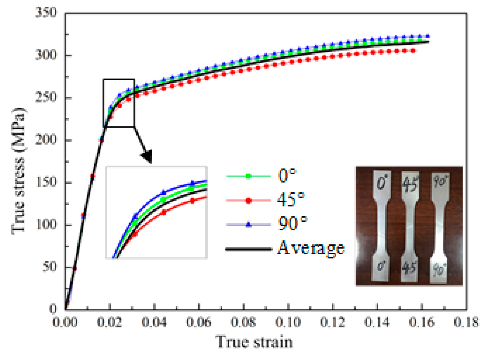
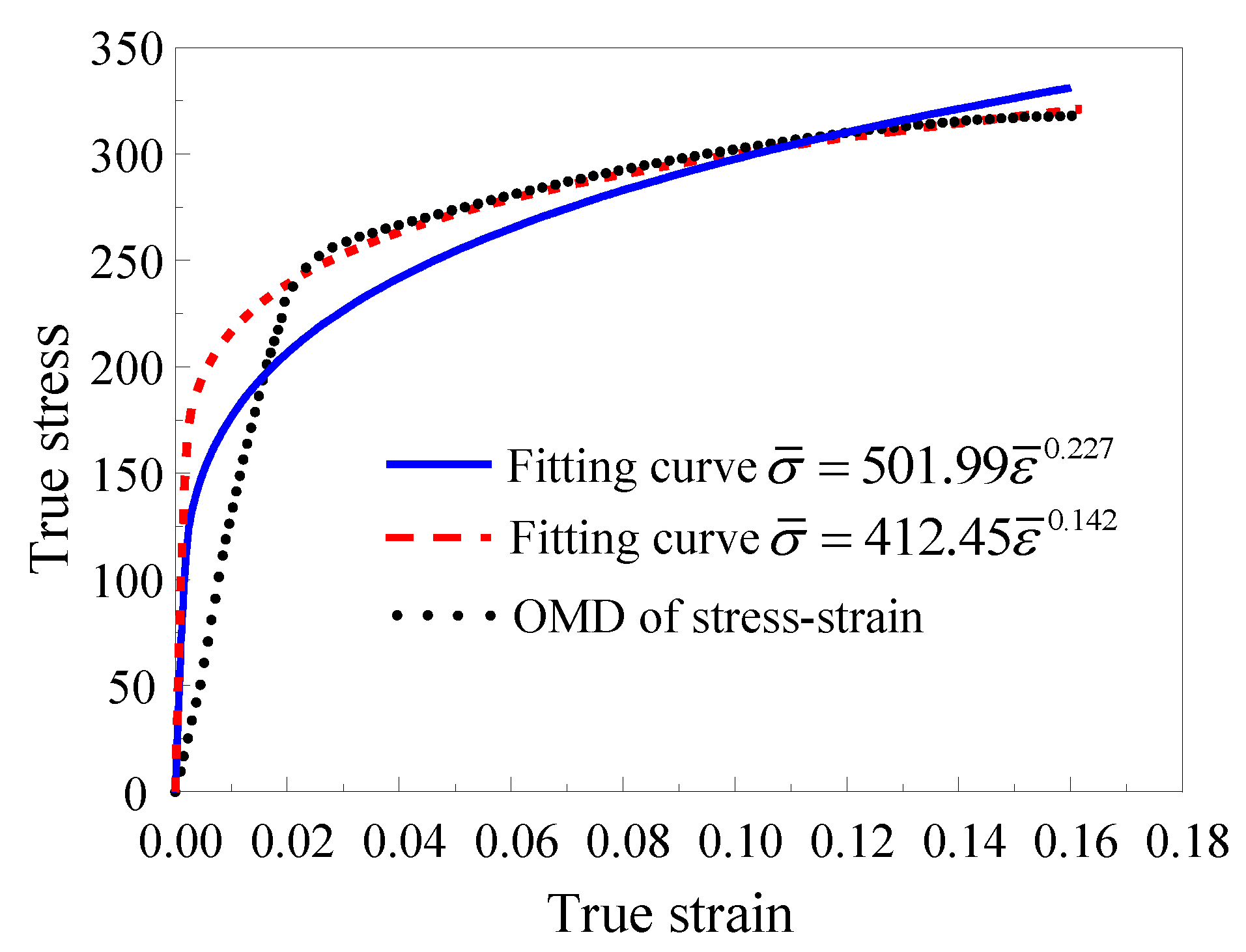
2. Uniaxial Tensile Tests

To obtain the true stress–strain curves of 6016-T4 aluminum alloy sheet, uniaxial tensile tests on the specimens in 0°, 45°, and 90° to the rolling direction were performed in a DNS100 microcomputer-controlled and universal material testing machine, and the direction of 0° is the rolling direction. The specimen had the strain gauge length of 55 mm, the section width of 15 mm, and thickness of 1 mm. The true stress–strain curves of different orientations were plotted by analyzing experimental data in Figure 1. It was found that the true stress–strain curves had the same trend in three directions, and the difference was not particularly significant. So, the average value of the stress at a certain strain in each direction was the final measured data of stress-strain.

The mechanical properties of 6016-T4 aluminum alloy sheet are shown in

Table 1. Uniaxial tensile properties of 6016-T4 aluminum alloy in different orientations.

Material Properties	Orientation
	0°	45°	90°
Yield stress (MPa)	253.8	242.2	258.8
Ultimate tensile strength (MPa)	318.1	306.0	323.1
Uniform elongation (%)	16.17	15.78	16.36
Anisotropic parameter (r)	0.824	0.803	0.818
Average value of r	0.812

, and the mechanical properties of the material in different directions were not much different. The anisotropic parameter (r-values) can be calculated by measuring the gauge length and width of the specimen before and after deformation. The r-values in three orientations were similar and less than 1, which indicated the strain of the sheet metal was greater in the thickness direction than that in width direction. In engineering, the average value is generally used as the anisotropic parameter of sheet metal [20].

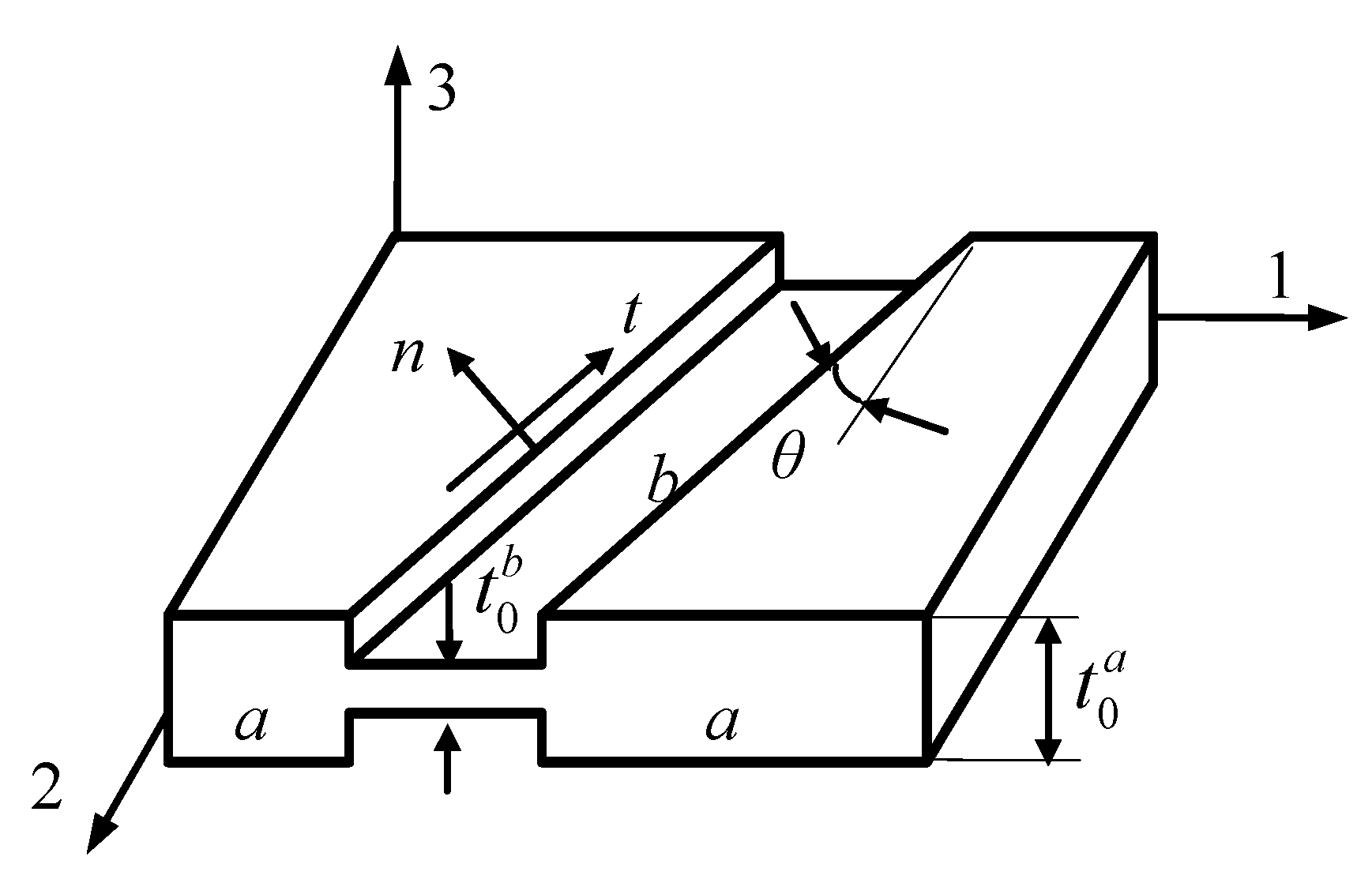
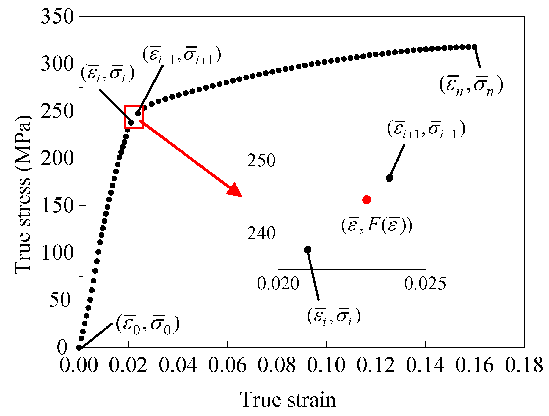
3. M–K Model Based on OMD of Stress–Strain

Marciniak and Kuczynski [13] proposed that necking is usually caused by geometric or structural imperfection and the original randomly distributed defects of sheet metal are assumed to be the weak area, i.e., the groove zone, and the thickness inhomogeneity is used to indicate the unevenness of the sheet metal. As shown in Figure 2, the sheet metal was divided into the uniform zone a and the weak zone b. The 1 and 2 axes indicate the principal stress directions in zone a, and the 3 axis indicates the thickness direction of the sheet metal. The normal and the tangential directions of the groove region are denoted by n and t, respectively. Moreover, the angle between the groove direction and the 2 direction is θ. For simplicity, the superscripts ‘a’ and ‘b’ are used to distinguish the corresponding variables in zones a and b.

In the M–K model, the force in the n direction is transmitted across zones a and b, therefore, the force equilibrium conditions can be obtained:

$$\{\begin{array}{l}{\sigma }_{nn}^a=f{\sigma }_{nn}^b\\ {\sigma }_{nt}^a=f{\sigma }_{nt}^b\end{array}$$

(1)

where ${\sigma }_{nn}$ and ${\sigma }_{nt}$ are, respectively, normal stress and shear stress in the groove local coordinate system (n-t coordinate system), and $f$ is the thickness inhomogeneity.

The equation can be obtained from Equation (1):

$${\sigma }_{nn}^a/{\sigma }_{nt}^a={\sigma }_{nn}^b/{\sigma }_{nt}^b$$

(2)

In addition, the relation of stress components between the n-t coordinate system and principal axis coordinate system (1-2 coordinate system) can be expressed as follows:

$$\{\begin{array}{l}{\sigma }_{nn}={\sigma }_{11}{\cos }^2\theta +{\sigma }_{22}{\sin }^2\theta +{\sigma }_{12}\sin 2\theta \\ {\sigma }_{nt}=({\sigma }_{22}-{\sigma }_{11})\sin \theta \cos \theta +{\sigma }_{12}\cos 2\theta \end{array}$$

(3)

There are not shear stress components in zone a, i.e., ${\sigma }_{12}^a$ = 0. Based on Equation (3), the stress components in zones a and b satisfy:

$$\{\begin{array}{l}{\sigma }_{nn}^a=A_a{\sigma }_1^a\\ {\sigma }_{nt}^a=B_a{\sigma }_1^a\end{array}$$

(4a)

$$\{\begin{array}{l}{\sigma }_{nn}^b=(A_b({\alpha }_b)+{\delta }_b\sin 2\theta ){\sigma }_{11}^b\\ {\sigma }_{nt}^b=(B_b({\alpha }_b)+{\delta }_b\cos 2\theta ){\sigma }_{11}^b\end{array}$$

(4b)

where, $\{\begin{array}{l}{\alpha }_a={\sigma }_2^a/{\sigma }_1^a\\ {\alpha }_b={\sigma }_{22}^b/{\sigma }_{11}^b\end{array}$ , $\{\begin{array}{l}{A}_a={\cos }^2\theta +{\alpha }_a{\sin }^2\theta \\ B_a=({\alpha }_a-1)\sin \theta \cos \theta \end{array}$, $\{\begin{array}{l}{A}_b({\alpha }_b)={\cos }^2\theta +{\alpha }_b{\sin }^2\theta \\ B_b({\alpha }_b)=({\alpha }_b-1)\sin \theta \cos \theta \end{array}$, ${\delta }_b={\sigma }_{12}^b/{\sigma }_{11}^b$.

By substituting Equation (4a) and (4b) into Equation (2), the equation can be found:

$${\delta }_b({\alpha }_b)=\frac{A_a{B}_b({\alpha }_b)-B_a{A}_b({\alpha }_b)}{B_a\sin 2\theta -A_a\cos 2\theta }$$

(5)

where ${\delta }_b$ is the function of ${\alpha }_b$.

In the M–K model, the strain paralleling to the groove in zone b is constrained by the strain in uniform zone a, so the compatibility condition can be given by

$$d{\epsilon }_{tt}^a=d{\epsilon }_{tt}^b$$

(6)

Moreover, the relation of strain increments between n-t and the 1-2 coordinates can be expressed as follows:

$$d{\epsilon }_{tt}=d{\epsilon }_{11}{\sin }^2\theta +d{\epsilon }_{22}{\cos }^2\theta -d{\epsilon }_{12}\sin 2\theta$$

(7)

There are not shear strain increments in zone a, i.e., $d{\epsilon }_{12}^a=0$. Based on Equation (7), the strain increments in zones a and b can satisfy:

$$\{\begin{array}{l}d{\epsilon }_{tt}^a=d{\epsilon }_1^a{\sin }^2\theta +d{\epsilon }_2^a{\cos }^2\theta \\ d{\epsilon }_{tt}^b=d{\epsilon }_{11}^b{\sin }^2\theta +d{\epsilon }_{22}^b{\cos }^2\theta -d{\epsilon }_{12}^b\sin 2\theta \end{array}$$

(8)

Combining with the plastic flow equation $d{\epsilon }_{ij}=d\overline{\epsilon }(\partial \overline{\sigma }/\partial {\sigma }_{ij})$ () and the equivalent stress of Hill 1948 ($\overline{\sigma }=\sqrt{3(1+r)/[2(2+r)]}\sqrt{{\sigma }_{11}^2-2r{\sigma }_{11}{\sigma }_{22}/(1+r)+{\sigma }_{22}^2+2(1+2r){\sigma }_{12}^2/(1+r)}$), the major and minor strain increments in zones a and b can be expressed:

$$\{\begin{array}{l}d{\epsilon }_1^a=R_1(2-R_2{\alpha }_a)d{\overline{\epsilon }}_a/{\phi }_a\\ d{\epsilon }_2^a=R_1(2{\alpha }_a-R_2)d{\overline{\epsilon }}_a/{\phi }_a\end{array}$$

(9a)

$$\{\begin{array}{l}d{\epsilon }_{11}^b=R_1(2-R_2{\alpha }_b)d{\overline{\epsilon }}_b/{\phi }_b({\alpha }_b)\\ d{\epsilon }_{22}^b=R_1(2{\alpha }_b-R_2)d{\overline{\epsilon }}_b/{\phi }_b({\alpha }_b)\\ d{\epsilon }_{12}^b=R_1{R}_3{\delta }_b({\alpha }_b)d{\overline{\epsilon }}_b/{\phi }_b({\alpha }_b)\end{array}$$

(9b)

where, $R_1=3(1+r)/[4(2+r)]$, $R_2=2r/(1+r)$, $R_3=4(1+2r)/(1+r)$, ${\phi }_a={\overline{\sigma }}_a/{\sigma }_1^a=\sqrt{2R_1(1-R_2{\alpha }_a+{\alpha }_a^2)}$, ${\phi }_b({\alpha }_b)={\overline{\sigma }}_b/{\sigma }_{11}^b=\sqrt{2R_1(1-R_2{\alpha }_b+{\alpha }_b^2+R_3{\delta }_b^2/2)}$.

By substituting Equations (8), (9a), and (9b) into Equation (6), the equation can be found:

$$d{\overline{\epsilon }}_b({\alpha }_b)=\frac{C_a}{C_b({\alpha }_b)}d{\overline{\epsilon }}_a$$

(10)

where, $\{\begin{array}{l}{C}_a=[(2-R_2{\alpha }_a){\sin }^2\theta +(2{\alpha }_a-R_2){\cos }^2\theta ]/{\phi }_a\\ C_b({\alpha }_b)=[(2-R_2{\alpha }_b){\sin }^2\theta +(2{\alpha }_b-R_2){\cos }^2\theta -R_3{\delta }_b({\alpha }_b)\sin 2\theta ]/{\phi }_b({\alpha }_b)\end{array}$, and $d{\overline{\epsilon }}_b$ is the function of ${\alpha }_b$.

The measured stress–strain curve can be reflected by a series of OMD of stress–strain $({\overline{\epsilon }}_i,{\overline{\sigma }}_i)$, which can be recorded as

$${\overline{\sigma }}_i=F({\overline{\epsilon }}_i)$$

(11)

When the OMD of stress–strain were recorded as n + 1 nodes and ${\overline{\epsilon }}_0<{\overline{\epsilon }}_1<\cdots <{\overline{\epsilon }}_i<{\overline{\epsilon }}_{i+1}<\cdots <{\overline{\epsilon }}_n$, as shown in Figure 3. For any equivalent strain $\overline{\epsilon }\ne {\overline{\epsilon }}_i$, firstly, determine the strain interval in which the strain is located, i.e., ${\overline{\epsilon }}_i<\overline{\epsilon }<{\overline{\epsilon }}_{i+1}$, then, the equivalent stress at any $\overline{\epsilon }$ can be calculated:

$$F(\overline{\epsilon })=\frac{\overline{\epsilon }-{\overline{\epsilon }}_i}{{\overline{\epsilon }}_{i+1}-{\overline{\epsilon }}_i}F({\overline{\epsilon }}_{i+1})+\frac{\overline{\epsilon }-{\overline{\epsilon }}_{i+1}}{{\overline{\epsilon }}_i-{\overline{\epsilon }}_{i+1}}F({\overline{\epsilon }}_i)$$

(12)

where the equivalent stress at any equivalent strain can be calculated by OMD of stress-strain.

In addition, based on the Equations (4a), (4b), and (12), ${\sigma }_{nn}^a=f{\sigma }_{nn}^b$ can be transformed to

$$A_{a}F({\overline{\epsilon }}_a){\phi }_b({\alpha }_b)=f(A_b+{\delta }_b({\alpha }_b)({\alpha }_b)\sin 2\theta )F({\overline{\epsilon }}_b){\phi }_a$$

(13)

where $F({\overline{\epsilon }}_a)$ and $F({\overline{\epsilon }}_b)$ can be calculated by Equation (12).

By substituting $f=t_b/t_a$, $f_0=t_0^b/t_0^a$, $t=t_0\exp ({\epsilon }_{33})$, and Equations (5), (10), and (12) into Equation (13), the iterative solution equation can be found:

$${\psi }_k({\alpha }_b^k)=A_{a}F({\overline{\epsilon }}_a^k){\phi }_b^k({\alpha }_b^k)-f_0\exp ({\epsilon }_{33}^{b(k)}({\alpha }_b^k)-{\epsilon }_3^{a(k)})(A_b^k({\alpha }_b^k)+{\delta }_b^k({\alpha }_b^k)\sin 2\theta )F({\overline{\epsilon }}_b^k){\phi }_a$$

(14)

The detailed steps of the Newton–Raphson method for solving the iterative solution equation (14) are described below:

According to the M–K theory, zone a is loaded proportionally, and the plastic deformation conforms to the total plastic theory. Firstly, assume the equivalent strain increment $d{\overline{\epsilon }}_a=\varsigma$ ($\varsigma$ is a very small constant, such as $\varsigma$ = 0.001) in zone a. When solving the iterative equation for the kth time, the equivalent stress based on OMD of stress–strain relation can be expressed as:

$$\{\begin{array}{l}F({\overline{\epsilon }}_a^k)=F({\overline{\epsilon }}_0+kd{\overline{\epsilon }}_a)\\ F({\overline{\epsilon }}_b^k)=F({\overline{\epsilon }}_0+{\displaystyle \sum _{k=1}^k\frac{C_a}{C_b^k({\alpha }_b^k)}}d{\overline{\epsilon }}_a)\end{array}$$

(15)

where, ${\overline{\epsilon }}_0$ is the prestrain of the sheet metal.

In this case, the iteration equation is:

$${\psi }_k({\alpha }_b^k)=A_{a}F({\overline{\epsilon }}_0+kd{\overline{\epsilon }}_a){\phi }_b^k({\alpha }_b^k)-f_0\exp ({\epsilon }_{33}^{b(k)}({\alpha }_b^k)-{\epsilon }_3^{a(k)})(A_b^k({\alpha }_b^k)+{\delta }_b^k({\alpha }_b^k)\sin 2\theta )F({\overline{\epsilon }}_0+{\displaystyle \sum _{k=1}^k\frac{C_a}{C_b^k({\alpha }_b^k)}}d{\overline{\epsilon }}_a){\phi }_a$$

(16)

where, $\{\begin{array}{l}{\epsilon }_3^{a(k)}=-k[(2R_1-R_1{R}_2){\alpha }_a+2R_1-R_1{R}_2]d{\overline{\epsilon }}_a/{\phi }_a\\ {\epsilon }_{33}^{b(k)}({\alpha }_b^k)=-{\displaystyle \sum _{k=1}^k[(2R_1-R_1{R}_2){\alpha }_b^k+2R_1-R_1{R}_2]d{\overline{\epsilon }}_b^k({\alpha }_b^k)/{\phi }_b^k({\alpha }_b^k)}\end{array}$.

Solving the iteration equation ${\psi }_k({\alpha }_b^k)=0$, Newton’s iteration formula is:

$${\alpha }_b^{k+1}={\alpha }_b^k-{\psi }_k({\alpha }_b^k)/{\psi }_k^{\prime }({\alpha }_b^k)$$

(17)

in Equation (17),

$$\begin{array}{l}{\psi }_k^{\prime }({\alpha }_b^k)=A_{a}F({\overline{\epsilon }}_0+kd{\overline{\epsilon }}_a)\frac{\partial {\phi }_b^k({\alpha }_b^k)}{\partial {\alpha }_b^k}-[f_0\exp (\frac{\partial {\epsilon }_{33}^{b(k)}({\alpha }_b^k)}{\partial {\alpha }_b^k}-{\epsilon }_3^{a(k)})(A_b^k({\alpha }_b^k)+{\delta }_b^k({\alpha }_b^k)\sin 2\theta )F({\overline{\epsilon }}_0+{\displaystyle \sum _{k=1}^k\frac{C_a}{C_b^k({\alpha }_b^k)}}d{\overline{\epsilon }}_a){\phi }_a+\\ \begin{array}{cc}& \end{array}\begin{array}{cc}& \end{array}{f}_0\exp ({\epsilon }_{33}^{b(k)}({\alpha }_b^k)-{\epsilon }_3^{a(k)})(\frac{\partial A_b^k({\alpha }_b^k)}{\partial {\alpha }_b^k}+\frac{\partial {\delta }_b^k({\alpha }_b^k)}{\partial {\alpha }_b^k}\sin 2\theta )F({\overline{\epsilon }}_0+{\displaystyle \sum _{k=1}^k\frac{C_a}{C_b^k({\alpha }_b^k)}}d{\overline{\epsilon }}_a){\phi }_a+\\ \begin{array}{cc}& \end{array}\begin{array}{cc}& \end{array}{f}_0\exp ({\epsilon }_{33}^{b(k)}({\alpha }_b^k)-{\epsilon }_3^{a(k)})(A_b^k({\alpha }_b^k)+{\delta }_b^k({\alpha }_b^k)\sin 2\theta )\frac{F({\overline{\epsilon }}_b^k)-F({\overline{\epsilon }}_b^{k-1})}{C_a\frac{d{\overline{\epsilon }}_a}{C_b^k({\alpha }_b^k)}\frac{\partial C_b^k({\alpha }_b^k)}{\partial {\alpha }_b^k}}{\phi }_a]\end{array}$$

(18)

Iteratively solve Equation (17) to $|{\alpha }_b^{k+1}-{\alpha }_b^k|\le eps$ ($eps$ is very small, such as $eps={10}^{-10}$), when the iterative equation converges, the unknown quantity ${\alpha }_b^k$ in zone b can be obtained.

Then, calculate ${\delta }_b^k({\alpha }_b^k)$, $d{\overline{\epsilon }}_b^k({\alpha }_b^k)$ based upon Equations (5) and (10), and check $d{\overline{\epsilon }}_b^k/d{\overline{\epsilon }}_a^k$. If $d{\overline{\epsilon }}_b^k/d{\overline{\epsilon }}_a^k\ge \lambda$ ($\lambda$ is an integer, such as $\lambda =10$), the formulas for calculating the major and minor strains when the sheet metal is necked are:

$$\{\begin{array}{l}{\epsilon }_{1(k)}^a={\epsilon }_{1(k-1)}^a+R_1(2-R_2{\alpha }_a)d{\overline{\epsilon }}_a/{\phi }_a\\ {\epsilon }_{2(k)}^a={\epsilon }_{2(k-1)}^a+R_1(2{\alpha }_a-R_2)d{\overline{\epsilon }}_a/{\phi }_a\end{array}$$

(19)

Otherwise, continue to solve equations ${\psi }_{k+1}({\alpha }_b^{k+1})=0$ by using Newton’s iteration method until the condition of $d{\overline{\epsilon }}_b^{k+1}/d{\overline{\epsilon }}_a^{k+1}\ge \lambda$ can be satisfied.

Change the groove angle θ, and the major and minor strains at different groove angles can be calculated separately. Finally, the minimum values of major and minor strains are taken as the ultimate strains.

Then, change ${\alpha }_a$ (${\alpha }_a\in [0,1]$), and the theoretical prediction of the major and minor strains under different loading paths can be obtained, and the FLC can be drawn.

The detailed steps of the Newton–Raphson method for calculating the ultimate strain are described below in the corresponding flow chart, as shown in Figure 4.

4. Experiments’ Determination on FLC

The FLC should include the loading path from uniaxial tension to plane strain to balanced biaxial tension, so that the complete FLC can be obtained. In previous studies, the numerical–experimental approach with the specimens of different shapes and widths was employed to calculate forming limits through uniaxial tensile, plane strain state, and biaxial tensile [44,45,46]. In this section, the punch-stretch tests for specimens of different shapes were simulated, then, the optimized specimens’ shape and punch-stretch test scheme were determined. The punch-stretch tests were carried out, and the experimental results were compared with the theoretical FLCs based on different stress–strain data.

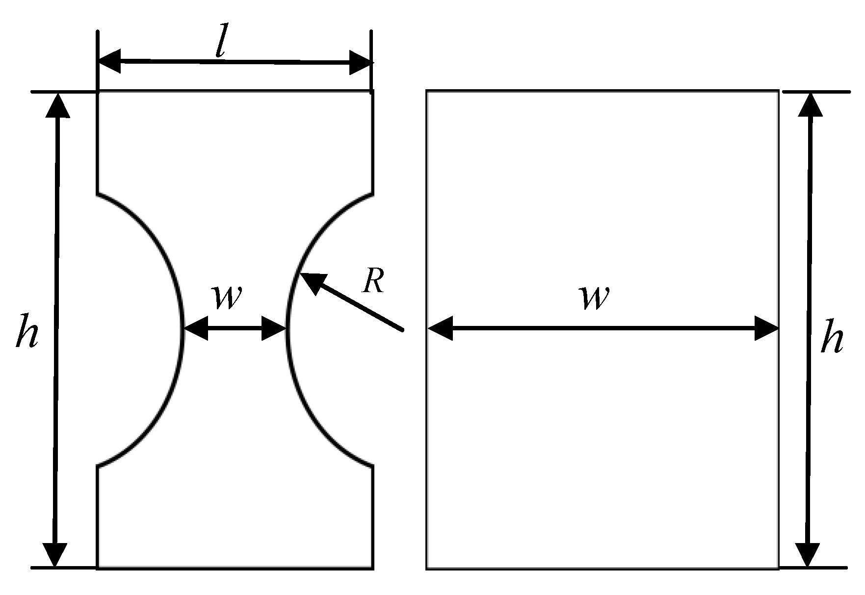
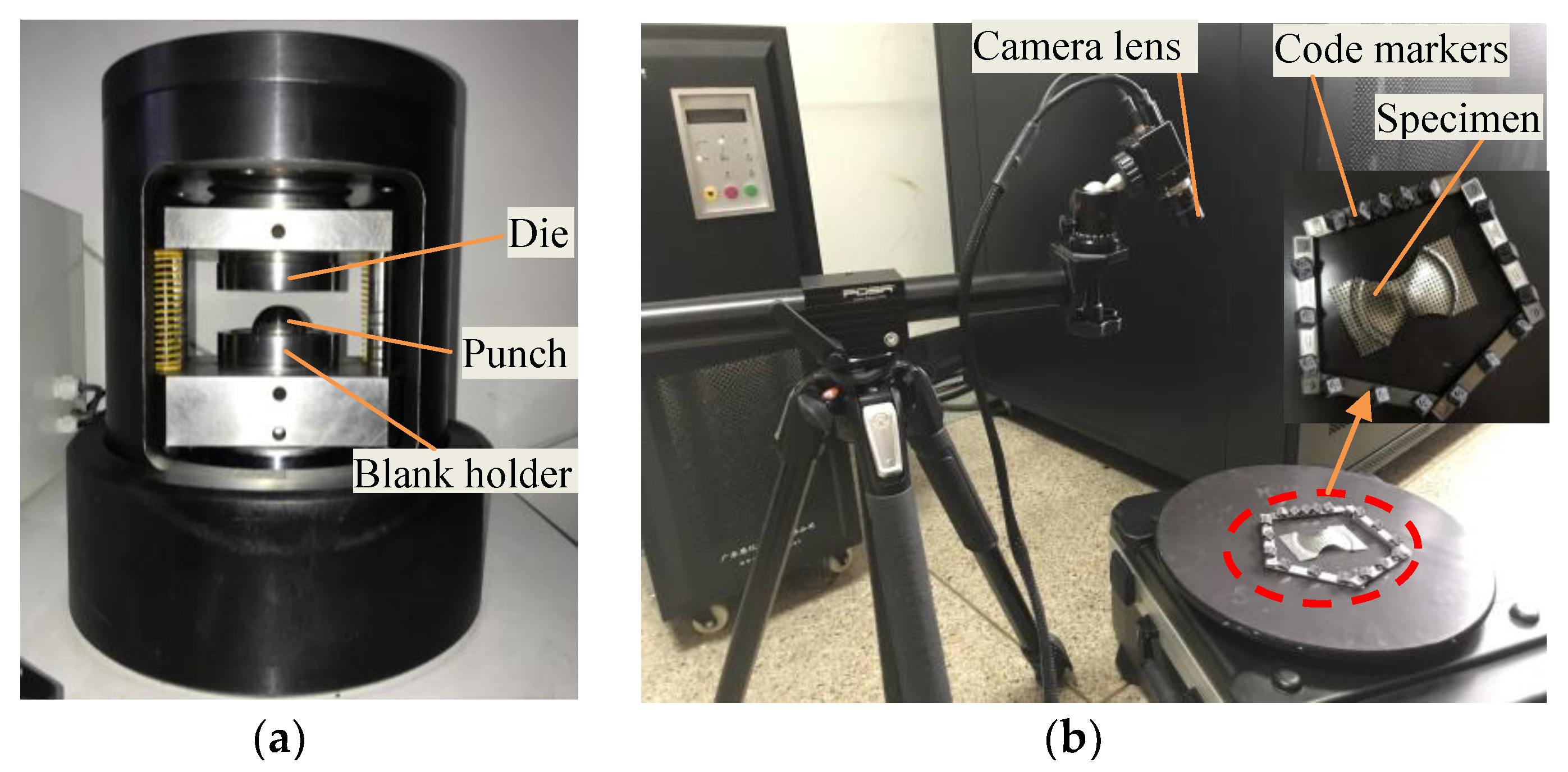
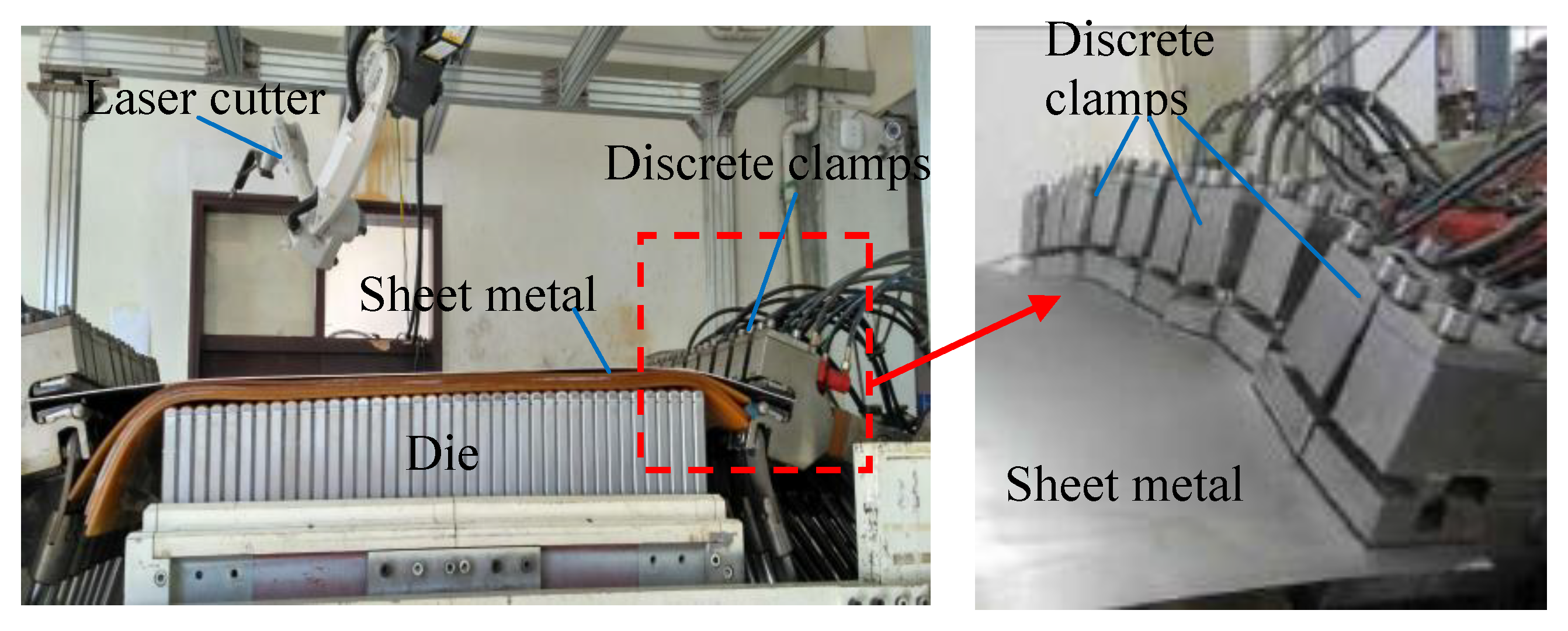
4.1. Numerical Simulations and Experiment Scheme

The numerical simulations were performed by Dynaform. Specimens of different widths and shapes were used to obtain the forming limits under different strain paths. In the simulation process, it was considered that the concave die, the blank holder, and the spherical punch were defined as the rigid body and meshed with R3D4 elements; the sheet metal can be deformed and meshed with S4R elements. In addition, the mesh size of all parts was 2 mm, and the symmetric constraints were loaded at the symmetric boundary of parts. The contact state between the contact pairs is decided by a master–slave algorithm, and the surfaces of the rigid body were defined as the master surface, while the surface of the deformed sheet metal was defined as the slave surface. The blanking force of 20 kN was applied to the blank holder. After the process parameters were set, the numerical simulation task was submitted for analysis, and the simulation results were analyzed in the post-processing program.

The punch-stretch test was widely used to obtain forming limits. The effective forming area of the specimen was used to design a rectangular strip, however, the numerical simulation results showed that the specimen with the small width was easily broken at the blank holder, as shown in Figure 5a. Since the rectangular specimen was subjected to the large concentrated stress at the blank holder, the large major strain appeared there, which may eventually result in the reduction of forming limits. In order to prevent failure from occurring at the blank holder region, the specimen was designed as dumbbell-shaped in the effective forming area, that is, the intermediate area was designed as the arc, which can smoothly transit from the center to both sides. The maximum value of the major strain of the dumbbell-shaped specimen appeared in center region, as shown in Figure 5.

Numerical simulation results of specimens with different sizes showed that, as the width of the specimen increased, the influence of the specimen shape on the simulation result was gradually weakened. As shown in Figure 5b, when the width of the effective formed area was about 60 mm, the simulation results of the two kinds of specimens were not much different. Considering the convenience and feasibility of processing and testing, the specimens with a large width were designed as rectangle. Therefore, the shape and size of the specimens were finally determined, and the experiment scheme is as shown in Figure 6 and

Table 2. Specimen sizes.

Dimension	1	2	3	4	5	6	7	8	9
w (mm)	10	15	20	30	40	50	60	70	80
R (mm)	40	37.5	35	30	25	20	*	*	*
l (mm)	40	42.5	45	50	55	60	*	*	*

, respectively, where h = 90 mm.

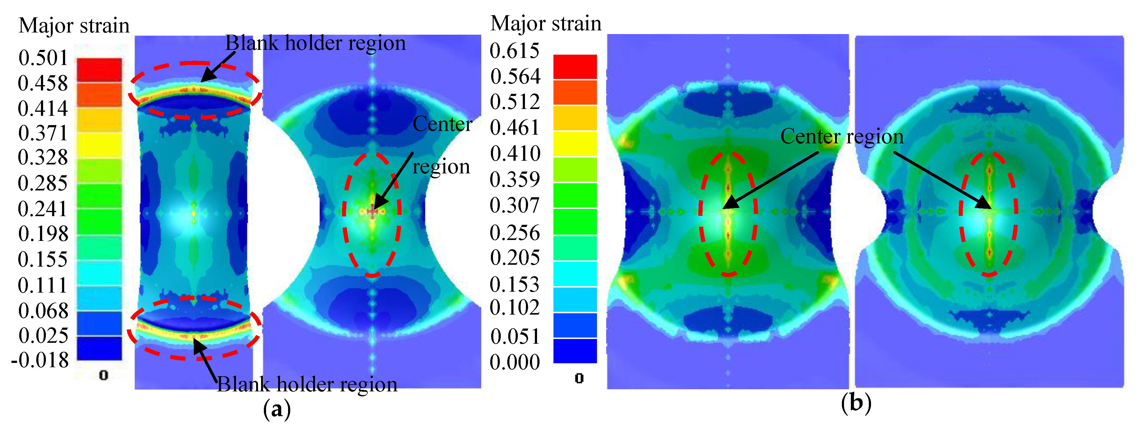
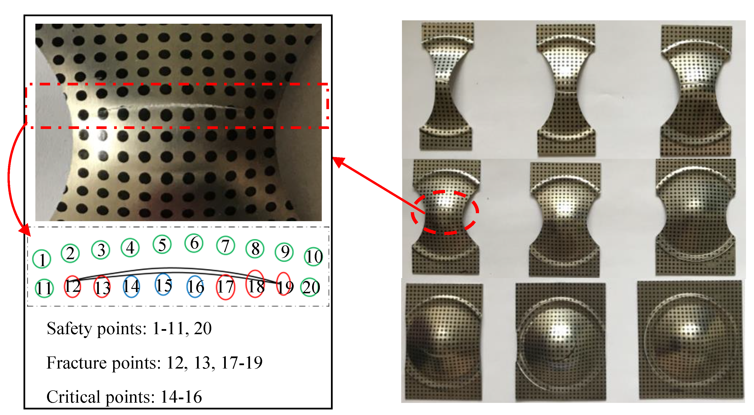
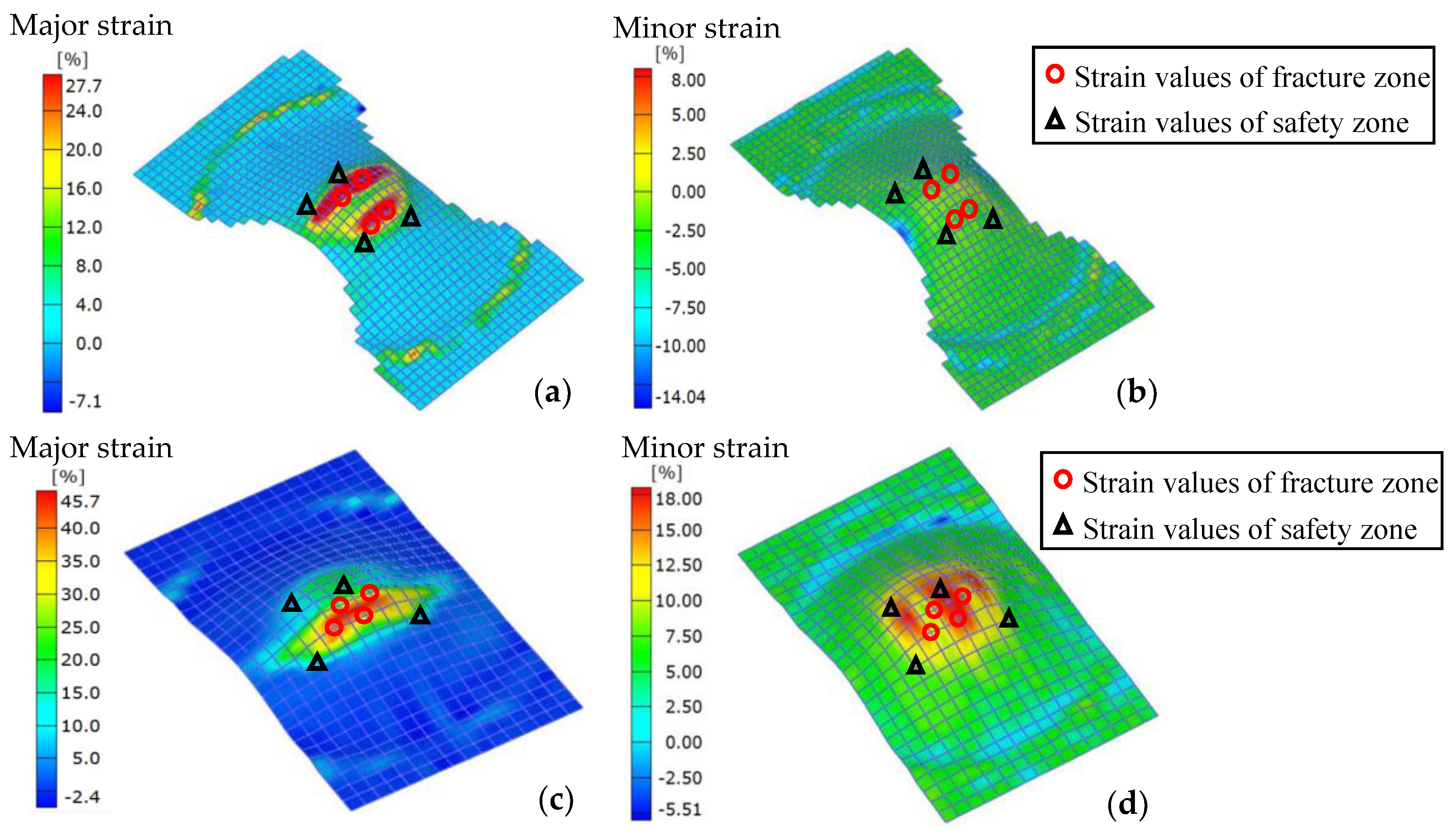
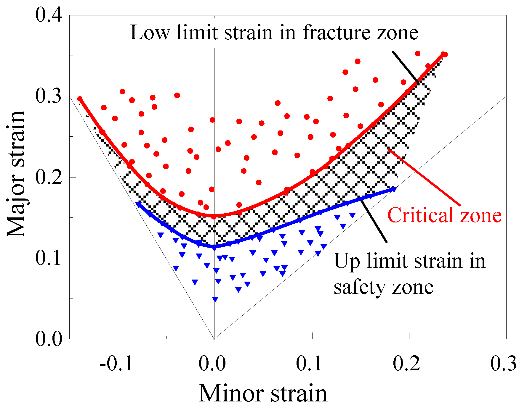
4.2. Analysis of Experiments Results

The punch-stretch tests were carried out. As shown in Figure 7a, the equipment adopted a two-stage hydraulic stretching and crimping system, which applied uniform blanking force to the specimens and improved the stability of the punch-stretch process. The ultimate strains of the sheet were obtained on the ARGUS optical strain gauge produced by GOM. This equipment can obtain the high-precision 3D full field strain data of the deformed sheet, and the main compositions of the test equipment are shown in Figure 7b.

In this experiment, the meshing method used was the circular grid division. The circular grid is the most widely used, and it is convenient to determine the major and minor strains. At the end of the deformation of the aluminum alloy sheet, the shape of the circular grid became the elliptical grid, and the major and minor strains of the sheet metal were calculated by the following formula:

$$\{\begin{array}{l}{\epsilon }_1=\ln (d_1/d_0)\\ {\epsilon }_2=\ln (d_2/d_0)\end{array}$$

(20)

where d₀ is the original diameter of the circular grid, and d₁ and d₂ are the long and short axes of the ellipse grid after deformation, respectively.

According to the designed test scheme, punch-stretch tests of different specimens were carried out. The deformed specimens are shown in Figure 8. According to the fracture position of the specimen and the deformation degree of the grid, the deformed regions of the sheet metal were divided into three categories: Fracture region, critical region, and safety region. It can be seen that the cracking degree of the specimen and the deformation degree of the mesh were different, so a mass of data needs to be extracted to predict the FLC of the sheet metal reasonably.

The ARGUS optical strain gauge can obtain the deformed mesh distribution on the surface of the deformed specimen. Then, the major and minor strains’ distributions of the deformed specimens can be further analyzed by the software. The major and minor strain of the specimens with the width of 30 mm and 60 mm are shown in Figure 9. The cracking degree of specimens with different sizes is different. Therefore, in order to predict the FLC of the 6016-T4 aluminum alloy, the strain data in the safety and fracture zones of specimens were extracted. It can be found that the major strains of the fracture zone were significantly larger than those of the safety zone, and the smaller the width of the specimen, the more likely the minor strain was negative value. The extraction locations of major and minor strains in the safety and fracture zones are also marked in Figure 9.

For the punch-stretch test, the major and minor strains in the safety and fracture zones are expressed in Figure 10. The strain data in the fracture and safety zones were extracted, and the strain data distributions were scattered, so it was difficult to present a clear FLC. The majority of strain data distributed in the fracture and safety zones, and very few strain data were located in the intermediate critical region. Instead, the FLC band was presented with a certain width. The two curves can be plotted to limit the dispersed strain points to a certain zone, that is, the critical zone is between the upper limit curve of the safety zone and the lower limit curve of the fracture zone. The FLC band can be regarded as the critical zone of fracture.

5. Results and Discussion

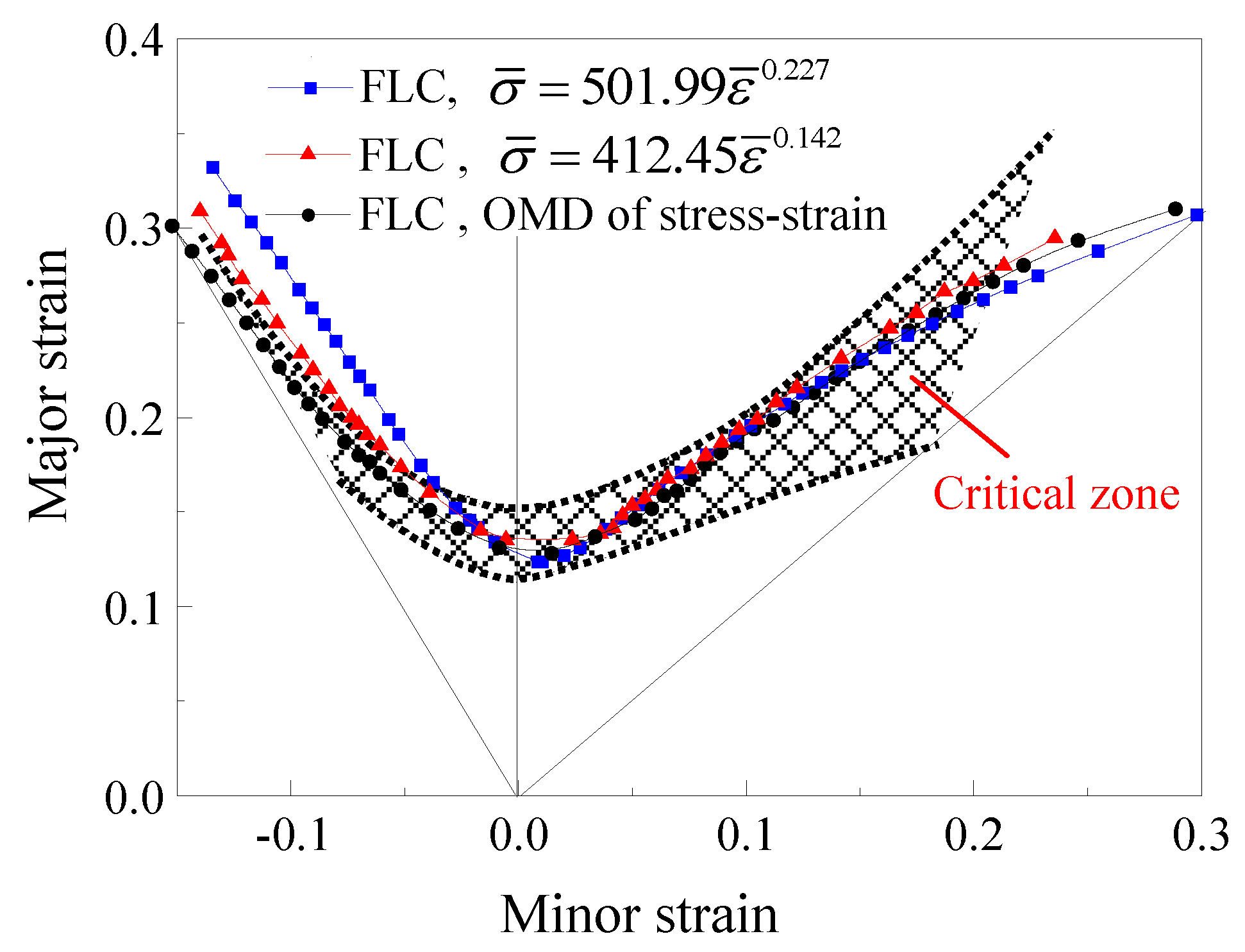
5.1. Comparison of FLCs Calculated by OMD of Stress–Strain and Power Function

Uniaxial tensile tests were carried out in the directions of 0°, 45°, and 90° with the rolling direction, and three sets of true stress–strain curves with little differences were obtained. In order to improve the accuracy of the experiment, the average values were taken as OMD of stress–strain, as shown in Figure 11. The equivalent stress at any equivalent strain based on OMD of stress–strain can be calculated by Equation (12). Then, the FLC based on OMD of stress–strain can be calculated by the theoretical derivation in the third section.

The power function stress–strain curve ($\overline{\sigma }=K{\overline{\epsilon }}^n$) was obtained by fitting experimental stress–strain data. The parameters K and n in power function based on fitting the complete stress–strain curve (including elastic and plastic deformation) were 501.99 MPa and 0.227, respectively. In addition, since the fracture occurred in the plastic deformation stage, the power function based on the stress–strain relation of plastic deformation stage was $\overline{\sigma }=412.45{\overline{\epsilon }}^{0.142}$, as shown in Figure 11. It can be seen that the power function of the stress–strain curve was restricted by the equation form, which deviated from the OMD of stress–strain.

The FLCs based on different stress–strain relations were calculated, and shown in Figure 12. It was found that the theoretical FLCs based on power function of stress–strain curves were higher than the experimental FLC under the negative-strain path. The left side of FLCs based on power functions of stress–strain curves was above the critical zone of punch-stretch tests, but the right side of FLC was in the critical zone measured by punch-stretch tests. Moreover, the theoretical FLC calculated based on the power function ($\overline{\sigma }=412.45{\overline{\epsilon }}^{0.142}$) was closer to the test value than that based on $\overline{\sigma }=501.99{\overline{\epsilon }}^{0.227}$. Finally, the theoretical FLC calculated by OMD of stress–strain was between the safety and fracture zones of punch-stretch tests, that is, the predicted major and minor strains were in the critical zone of the necking. By comparison, it was found that the stress–strain curves of sheet metal had significant impact on FLC under the negative-strain path, and the theoretical FLC based on OMD of stress–strain was more consistent with the experimental results, which verified the accuracy and superiority of the proposed method in this paper.

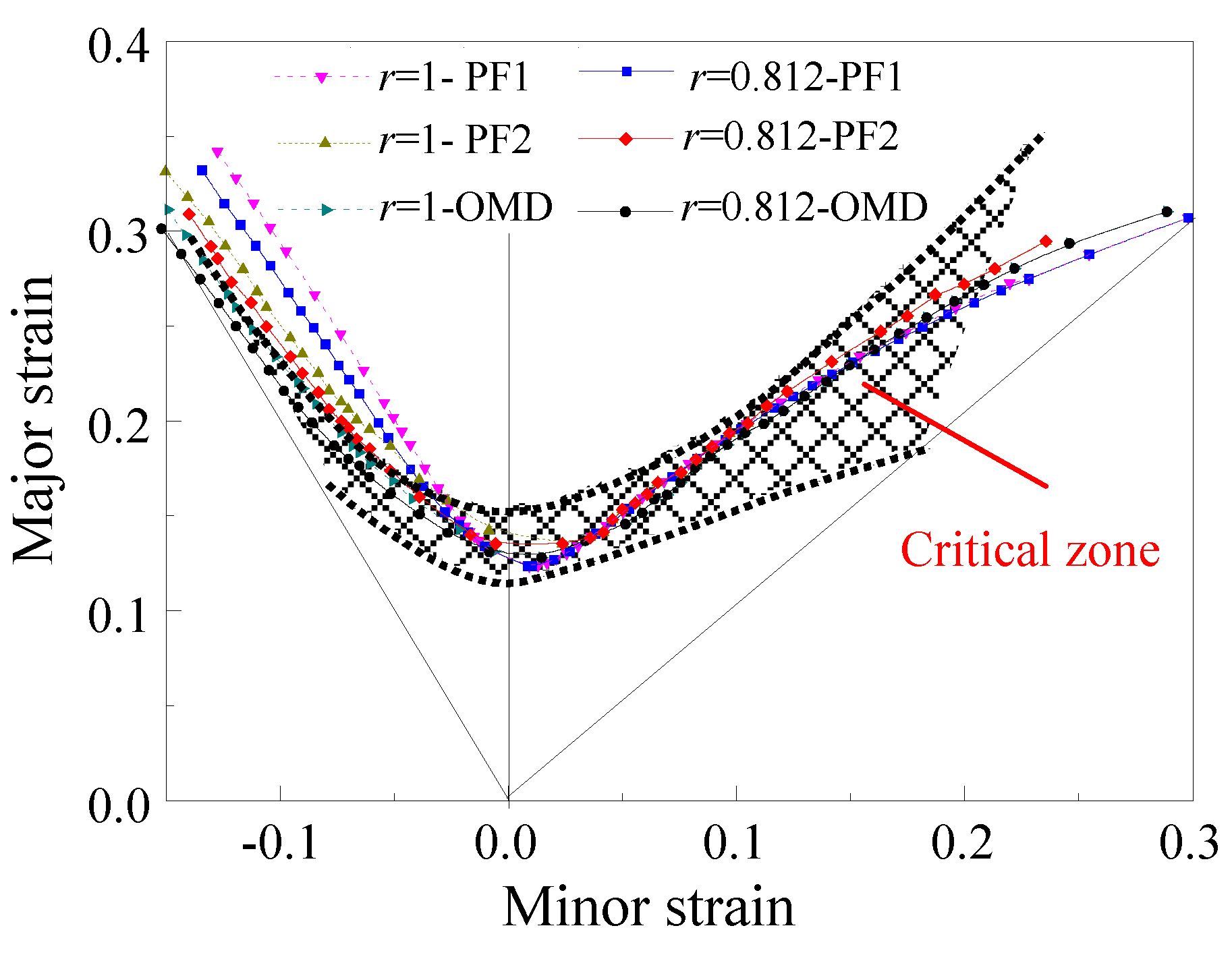
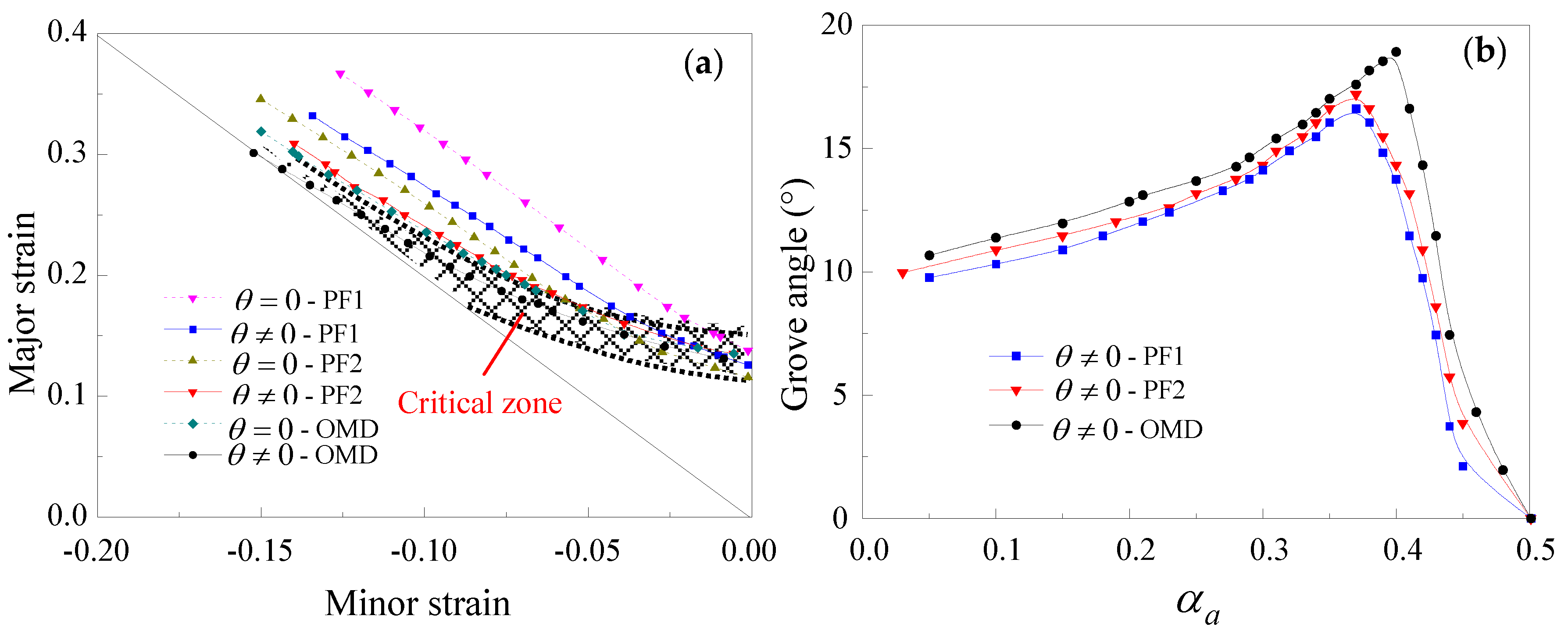
5.2. Influence of Anisotropic Parameter and Groove Angle on FLCs

It is well known that the von Mises yield function considers the anisotropic parameter (r) equals 1, and the Hill 1948 yield function can include a non-zero anisotropic parameter. In Figure 13, PF1 and PF2 represent power functions by fitting the complete ($\overline{\sigma }=501.99{\overline{\epsilon }}^{0.227}$) and plastic deformation stress–strain curve ($\overline{\sigma }=412.45{\overline{\epsilon }}^{0.142}$), respectively. It was found that the anisotropic parameter had significant impact on FLC, and the ultimate strains were greater when r = 1 than when r < 1 in three prediction methods, especially, in the negative-strain path. It can be found from Table 1 that the aluminum alloy 6016-T4 was anisotropy. It was more reasonable to predict the FLCs by using r < 1. Moreover, the FLCs calculated by the M-K model combining OMD of stress–strain were more consistent with the punch-stretch test results than those based on power functions.

From the above analysis, it can be seen that, when the FLCs of the sheet metal were predicted by the M–K model combining with OMD of stress–strain and power functions, the FLCs under the negative-strain path were observably influenced by stress–strain relation. The FLCs under the negative-strain paths were minimized under non-zero groove angles. However, the FLCs under the positive-strain path were minimized when the groove angle was zero. In order to analyze the effect of the groove angle on the FLCs, the left side of the FLC was calculated with zero and non-zero groove angles, as shown in Figure 14a. It can be seen that the FLCs predicted by three methods were higher in zero angle than in non-zero angle, and the predicted FLCs were closer to the experimental data in non-zero groove angle. Therefore, in order to accurately predict the FLCs, the FLCs in the negative-strain paths should be calculated at non-zero groove angles. In addition, when the ultimate strains take the minimum values, the variations of groove angle with different strain paths are shown in Figure 14b. It was found that, when the ultimate strain took the minimum value, the groove angle increased firstly and then decreased when sheet deformations changed from the uniaxial tension to the plane strain state. The groove angle at the plane strain state was zero with the minimum strain, which was consistent with the minimum value of the forming limit in the right side when the groove angle was zero. Therefore, the groove angle had a certain influence on the left side of the FLC.

6. Application of FLC in the Stretch-Forming Process Based on Loading at Multi-Positions

The FLC was applied to evaluate whether the three-dimensional curved parts appear in the fracture defect during the stretch-forming process, and the fracture defect can be predicted by FLC. The stretch-forming process is an important method for forming three-dimensional curved parts. It is widely used to form the skin parts of aircraft and spacecraft, the front of high-speed trains, the outer plates of ships, and the large-curvature curved parts of modern buildings. The integral clamps in a conventional stretch-forming process were replaced by discrete clamps based on loading at multi-positions, as shown in Figure 15. The displacement load was applied at a series of discrete clamps on the two ends of the sheet metal, and the load of each loading point was controlled in real time, so that the deformed sheet could actively deform along with the die profile. The discrete clamps made the sheet metal bend and stretch according to the die surface, and ultimately realized the complete fit between the sheet metal and the die, forming high-precision surface parts.

The loading trajectory had a great influence on forming results of a curved-surface part, and stress and strain distributions of curved parts were different under different loading trajectories. In this section, numerical simulation and experimental verification were carried out for spherical parts under different loading paths. Combining with the prediction of sheet metal-forming limits, the fracture defects of curved-surface parts were predicted by FLC obtained by the proposed method.

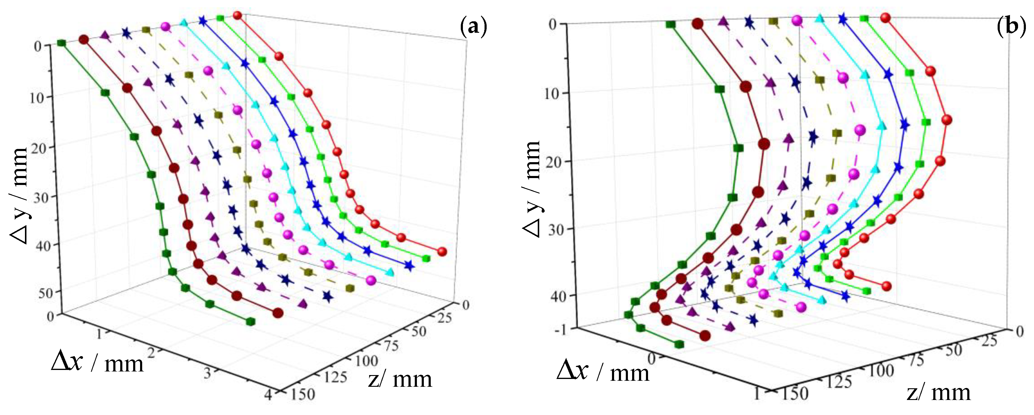
6.1. Loading Trajectories for the Stretch-Forming Process Based on Loading at Multi-Positions

It is well known that the loading trajectories of the discrete clamps have great influence on the forming precision and quality of a three-dimensional curved part. From a geometric point of view, there are countless loading trajectories from flat sheet to three-dimensional curved parts. In order to compare and analyze the influence of different loading paths on the forming results of curved parts, the stretch-forming process based on equal and variable elongation was designed to form curved parts.

Since the influence of the sheet width on the longitudinal strain was relatively small, it was considered that the sheet metal was composed of several longitudinal strips with the same width as the discrete clamps, and the corresponding strips were deformed by controlling the displacements at the loading points. The deformation process of ith longitudinal strip is shown in Figure 16. The loading trajectory was the moving locus of the end of the material line during the process. It was seen that the material line changed from its initial length to an intermediate length and finally to the length corresponding to the arc length of the stretching die. In the stretch-forming process based on equal elongation (SF-e), it was assumed that the elongation of the longitudinal strip of the sheet metal was equal, and the displacement of each loading point was calculated separately. In the stretch-forming process based on variable elongation (SF-v), the elongations of the longitudinal strips of the sheet metal varied and were determined by cubic functions in the forming process. The details for deriving the process of equal elongation loading mode and variable elongation loading mode can be found in reference [43].

When the sheet length was 400 mm, the sheet width was 300 mm and the spherical part with the radius of 500 mm was formed in numerical simulations. The loading trajectories of different loading points in different loading methods (SF-e and SF-v) are shown in Figure 17.

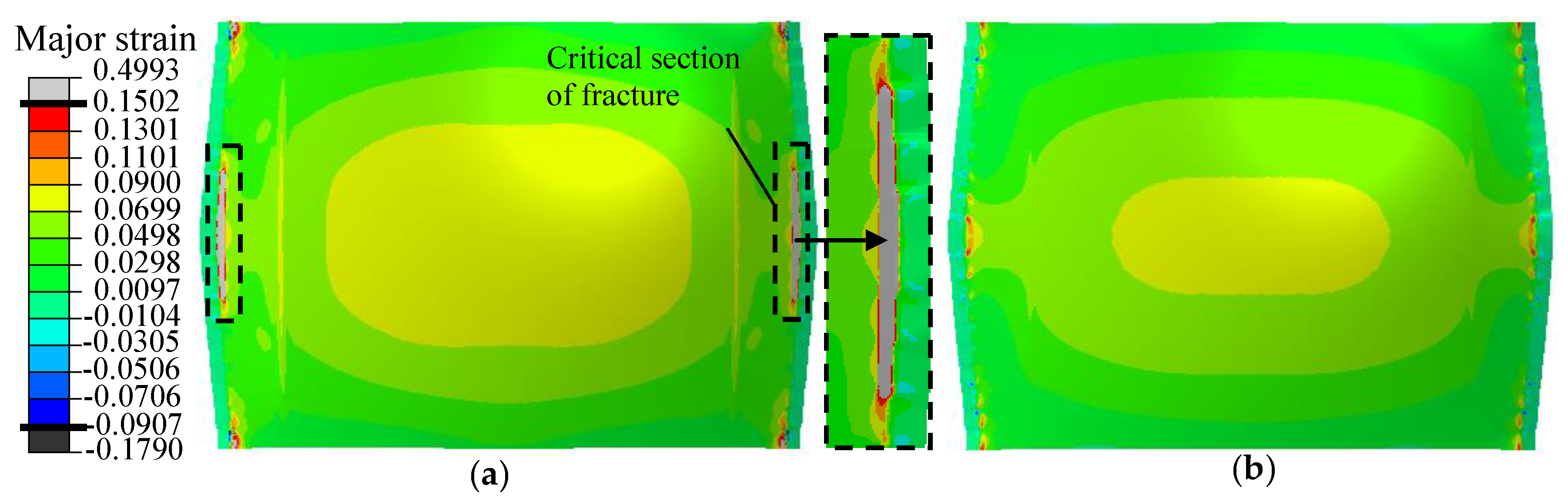
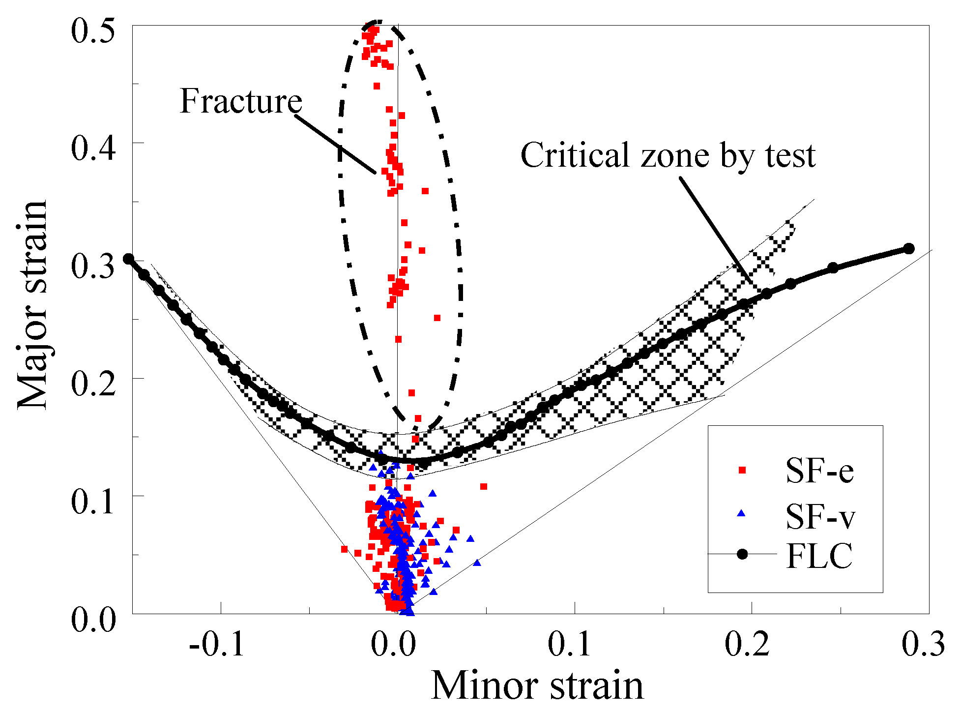
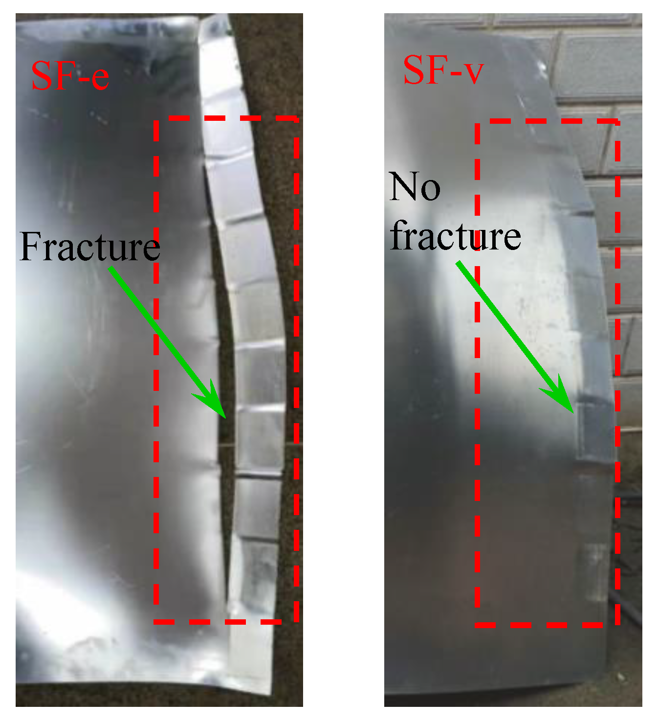
6.2. Numerical Simulation Results and Experimental Validation

The spherical parts with the radius of 500 mm were formed by two loading methods, and the major strain distributions of the numerical simulations are shown in Figure 18. It can be seen from Figure 18 that when different loading trajectories were adopted to form spherical parts of the same curvature, the major strain distributions in the effective formed region had the same tendency, but the spherical part in SF-v had more uniform strain distribution than in SF-e. The maximum major strain of the spherical part in SF-e was 0.4993, which was much larger than 0.1502 in SF-v. Moreover, the spherical part formed by SF-e had the larger strains in the middle region that was adjacent to the discrete clamps, and the larger strains may have caused the formation of fracture defect in the region. The appearance of the fracture defect reduced the accuracy of the curved part and even produced unacceptable curved parts.

In order to study the fracture defect under different loading modes, the major and minor strains of the spherical parts in a critical section of fracture were extracted. It can be seen from Figure 19 that, in SF-e, the strains in a critical section of fracture exceeded the theoretically calculated ultimate strains and were located in the fracture region measured by experiment. The regions of strain points above the FLC appeared in fracture defect, and the spherical part in SF-e was prone to fracture in plane strain state. The fracture defects reduced the accuracy of the formed parts, and the defective parts were manufactured in SF-e. However, in SF-v, all strain points in the critical section of fracture were below the FLC and were located in the safe region measured by experiment, which indicated that the possibility of fracture defect in SF-v was especially small. Meanwhile, it was found that the FLC predicted by combining the M–K theory and the OMD of stress–strain can quantitatively analyze the fracture defect, which has certain guiding significance for the sheet-forming process.

In order to verify the numerical simulation results of the stretch-forming process in different loading trajectories, the stretch-forming experiments for spherical parts of aluminum alloy 6016-T4 were carried out on a homemade apparatus by Jilin University, as shown in Figure 15. The critical sections of fracture of experimental parts are shown in Figure 20. It can be seen that the large deformation was produced in SF-e, and the severe fracture defect appeared in the center region that was adjacent to the discrete clamps. However, in SF-v, as indicated by experimental result, the target surface part was perfectly manufactured without fracture defect. In conclusion, the experiment results verified the accuracy of the numerical simulation and FLC prediction, and the fracture defect appeared in the region where the strain points exceeded the theoretically calculated ultimate strains.

7. Conclusions

In this paper, the new method by directly utilizing OMD of stress–strain relation in the M–K model was proposed to predict the FLC of an aluminum alloy sheet, and the predicted FLC in this method was compared with that of the M–K model based on power functions and punch-stretch tests. In addition, the predicted FLC in the proposed method was used to analyze the sheet formability in the stretch-forming process. The conclusions of this paper can be summarized as follows:

(1) In this paper, the new method by directly utilizing OMD of stress–strain relation in the M–K model was proposed to predict FLC of an aluminum alloy sheet, and the detailed theoretical derivations for calculating forming limits were presented.

(2) The stress–strain curve had significant effect on the FLC prediction of sheet metal. The power functions were fitted by the OMD of stress–strain, but the true stress–strain relation of the material was not strictly reflected by power function, which may have affected the prediction results of the sheet-forming limits. However, the OMD of stress–strain can strictly reflect the true stress–strain relation of the material, so the FLC prediction results based on OMD of stress–strain can be more accurate.

(3) By comparing the FLCs based on OMD of stress–strain and power functions with experiment result, it was found that the theoretical FLCs based on power functions were higher on the left side than the experimental FLC, and the right side of FLC was in the critical zone measured by experiment. However, the theoretical FLC based on OMD of stress–strain were in the critical zone measured by experiment. The predicted FLC in the proposed method were more consistent with the experimental results, and the accuracy and superiority of the proposed method were verified in this paper.

(4) Anisotropic parameter affected the prediction accuracy of FLC, and the groove angle had significant effect on the FLC under the negative-strain path. The predicted forming limits with zero groove angle were higher than that when the groove angle was not zero. In this paper, the forming limits calculated in the conditions of r < 1 and were more consistent with the experimental FLC.

(5) The FLC calculated by the proposed method was applied to analyze sheet formability in the stretch-forming process, and the predicted results of FLC were verified by numerical simulations and experiment of the stretch-forming process. The fracture tendency of the weakened region of the formed parts could be intuitively visualized and quantitatively analyzed in FLD, which had certain guiding significance for fracture judgment in the sheet-forming process.

References

1. Dursun, T.; Soutis, C. Recent developments in advanced aircraft aluminum alloys. Mater. Des. 2014, 56, 862–871. [Google Scholar] [CrossRef]
2. Eyckens, P.; Bael, A.V.; Houtte, P.V. Marciniak-Kuczynski type modelling of the effect of through-thickness shear on the forming limits of sheet metal. Int. J. Plast. 2009, 25, 2249–2268. [Google Scholar] [CrossRef]
3. Cai, Z.Y.; Wang, S.H.; Xu, X.D.; Li, M.Z. Numerical simulation for the multi-point stretch forming process of sheet metal. J. Mater. Process. Technol. 2009, 209, 396–407. [Google Scholar] [CrossRef]
4. Cai, Z.Y.; Liang, X.B.; Yang, Z.; Li, X.J. Force-controlled sheet metal stretch forming process based on loading at discrete points. Int. J. Adv. Manuf. Technol. 2007, 93, 1781–1789. [Google Scholar] [CrossRef]
5. Kim, W.J.; Sa, Y.K.; Kim, H.K.; Yoon, U.S. Plastic forming of the equal-channel angular pressing processed 6061 aluminum alloy. Mater. Sci. Eng. 2008, 487, 360–368. [Google Scholar] [CrossRef]
6. Yang, H.; Fan, X.; Sun, Z.; Guo, L.; Zhan, M. Recent developments in plastic forming technology of titanium alloys. Sci. China Technol. Sci. 2011, 54, 490–501. [Google Scholar] [CrossRef]
7. Aghaie-Khafri, M.; Mahmudi, R. Predicting of plastic instability and forming limit diagrams. Int. J. Mech. Sci. 2004, 46, 1289–1306. [Google Scholar] [CrossRef]
8. Lopes, A.B.; Rauch, E.F.; Gracio, J.J. Textural vs. structural plastic instabilities in sheet metal forming. Acta Mater. 1999, 47, 859–866. [Google Scholar] [CrossRef]
9. Watanabe, I.; Terada, K. A method of predicting macroscopic yield strength of polycrystalline metals subjected to plastic forming by micro-macro de-coupling scheme. Int. J. Mech. Sci. 2010, 52, 343–355. [Google Scholar] [CrossRef]
10. Chen, M.H.; Gao, L.; Wang, H. Research progresses on sheet metal forming limit stress diagram. China Mech. Eng. 2005, 16, 1593–1597. [Google Scholar]
11. Ding, J.; Zhang, C.; Chu, X.; Zhao, G.; Leotoing, L.; Guines, D. Investigation of the influence of the initial groove angle in the M–K model on limit strains and forming limit curves. Int. J. Mech. Sci. 2015, 98, 59–69. [Google Scholar] [CrossRef]
12. Prasad, D.; Kaan, I.; Raja, M. The effects of anisotropic yield functions and their material parameters on prediction of forming limit diagrams. Int. J. Solids Struct. 2012, 49, 3528–3550. [Google Scholar] [Green Version]
13. Hu, Q.; Li, X.F.; Chen, J. New robust algorithms for Marciniak-Kuczynski model to calculate the forming limit diagrams. Int. J. Mech. Sci. 2018, 148, 293–306. [Google Scholar] [CrossRef]
14. Swift, H.W. Plastic instability under plane stress. J. Mech. Phys. Solids 1952, 1, 1–18. [Google Scholar] [CrossRef]
15. Hill, R. On discontinuous plastic states, with special reference to localized necking in thin sheets. J. Mech. Phys. Solids 1952, 1, 19–30. [Google Scholar] [CrossRef]
16. Jaamialahmadi, A.; Kadkhodayani, M. A modified Storen-Rice bifurcation analysis of sheet metal forming limit diagrams. J. Appl. Mech. 2012, 79, 061004. [Google Scholar] [CrossRef]
17. Manopulo, N.; Hora, P.; Peters, P.; Gorji, M.; Barlat, F. An extended Modified Maximum Force Criterion for the prediction of localized necking under non-proportional loading. Int. J. Plast. 2015, 75, 189–203. [Google Scholar] [CrossRef]
18. Morales-Palma, D.; Martínez-Donaire, A.J.; Vallellano, C. On the use of Maximum Force Criteria to predict localised necking in metal sheets under stretch-bending. Metals 2017, 7, 469. [Google Scholar] [CrossRef]
19. Marciniak, Z.; Kuczynski, K. Limit strains in the processes of stretch-forming sheet metal. Int. J. Mech. Sci. 1967, 9, 609–612. [Google Scholar] [CrossRef]
20. Butuc, M.C.; Gracio, J.J.; Barata, D.R. A theoretical study on forming limit diagrams prediction. J. Mater. Proc. Technol. 2003, 142, 714–724. [Google Scholar] [CrossRef]
21. Yang, X.Y.; Lang, L.H.; Liu, K.N.; Cai, G.C.; Guo, C. Prediction of forming limit diagram of AA7075-O aluminum alloy sheet based on modified M-K model. J. Beijing Univ. Aeronaut. Astronaut. 2015, 41, 675–679. [Google Scholar]
22. Wang, H.B.; Xu, Y.H. Sheet forming limit based on shear failure criterion under different constitutive relations. J. North. China Univ. Technol. 2017, 29, 61–68. [Google Scholar]
23. Le, K.C.; Piao, Y. Thermodynamic dislocation theory: Size effect in torsion. Int. J. Plast. 2019, 115, 56–70. [Google Scholar] [CrossRef]
24. Le, K.C.; Tran, T.M.; Langer, J.S. Thermodynamic dislocation theory of adiabatic shear banding in steel. Scr. Mater. 2018, 149, 62–65. [Google Scholar] [CrossRef] [Green Version]
25. Langer, J.S.; Bouchbinder, E.; Lookman, T. Thermodynamic theory of dislocation-mediated plasticity. Acta Mater. 2010, 58, 3718–3732. [Google Scholar] [CrossRef] [Green Version]
26. Du, P.M.; Lang, L.H.; Liu, B.S.; Gao, C. Theoretical prediction and parameter influence of FLDs based on M-K model. J. Plast. Eng. 2011, 18, 84–89. [Google Scholar]
27. Hou, B.; Yu, Z.Q.; Li, S.H.; Lin, Z.Q. Prediction of forming limit diagram of aluminum sheet at elevated temperatures. Mater. Sci. Technol. 2009, 17, 616–619. [Google Scholar]
28. Nader, A.; Farhang, P.; John, C. Forming of AA5182-O and AA5754-O at elevated temperatures using coupled thermo-mechanical finite element models. Int. J. Plast. 2007, 23, 841–875. [Google Scholar]
29. Barata, D.R.; Barlat, F.; Jalinier, J.M. Prediction of the forming limit diagrams of anisotropic sheets in linear and non-linear loading. Mater. Sci. Eng. 1985, 68, 151–164. [Google Scholar] [CrossRef]
30. Li, X.; Guo, G.; Xiao, J.; Song, N.; Li, D. Constitutive modeling and the effects of strain-rate and temperature on the formability of Ti-6Al-4V alloy sheet. Mater. Des. 2014, 55, 325–334. [Google Scholar] [CrossRef]
31. Chu, G.N.; Lin, Y.L.; Song, W.N.; Zhang, L. Forming limit of FSW aluminum alloy blank based on a new constitutive model. Acta Metal. Sin. 2017, 53, 114–122. [Google Scholar]
32. Zhang, H.; Zhang, H.; Li, F.Q.; Cao, J. A novel damage model to predict ductile fracture behavior for anisotropic sheet metal. Metals 2019, 9, 595. [Google Scholar] [CrossRef]
33. Woo, M.A.; Song, W.J.; Kang, B.S.; Kim, J. Acquisition and evaluation of theoretical forming limit diagram of Al 6061-T6 in electrohydraulic forming process. Metals 2019, 9, 401. [Google Scholar] [CrossRef]
34. Tomáš, m.; Evin, E.; Kepič, J.; Hudák, J. Physical modelling and numerical simulation of the deep drawing process of a box-shaped product focused on material limits determination. Metals 2019, 9, 1058. [Google Scholar] [CrossRef]
35. Pepelnjak, T.; Barišić, B. Computer-assisted engineering determination of the formability limit for thin sheet metals by a modified Marciniak method. J. Strain Anal. Eng. Des. 2009, 44, 459–472. [Google Scholar] [CrossRef]
36. Nakazima, K.; Kikuma, T.; Hasuka, K. Study on the formability of steel sheets. Yawata Tech. Rep. 1971, 284, 678–680. [Google Scholar]
37. Marciniak, Z.; Kuczynski, K.; Pokora, T. Influence of the plastic properties of the material on the forming limit diagram for sheet metal tension. Int. J. Mech. Sci. 1973, 15, 789–800. [Google Scholar] [CrossRef]
38. Wang, S.H.; Cai, Z.Y.; Li, M.Z. Numerical investigation of the influence of punch element in multi-point stretch forming process. Int. J. Adv. Manuf. Technol. 2010, 49, 475–483. [Google Scholar] [CrossRef]
39. Hardt, D.E.; Chung, K.; Richmond, O. In process control of strain in a stretch forming process. J. Eng. Mater. Technol. 2001, 123, 497–503. [Google Scholar] [CrossRef]
40. Peng, J.; Li, W.; Han, J.; Wan, M.; Meng, B. Kinetic locus design for longitudinal stretch forming of aircraft skin components. Int. J. Adv. Manuf. Technol. 2016, 86, 3571–3582. [Google Scholar] [CrossRef]
41. Cai, Z.Y.; Wang, S.H.; Li, M.Z. Numerical investigation of multi-point forming process for sheet metal: Wrinkling, dimpling and springback. Int. J. Adv. Manuf. Technol. 2008, 37, 927–936. [Google Scholar] [CrossRef]
42. Cai, Z.Y.; Yang, Z.; Che, C.J.; Li, M.Z. Minimum deformation path sheet metal stretch-forming based on loading at discrete points. Int. J. Adv. Manuf. Technol. 2016, 87, 2683–2692. [Google Scholar] [CrossRef]
43. Yang, Z.; Cai, Z.Y.; Che, C.J.; Li, M.Z. Numerical simulation research on the loading trajectory in stretch forming process based on distributed displacement loading. Int. J. Adv. Manuf. Technol. 2016, 82, 1353–1362. [Google Scholar] [CrossRef]
44. Petek, A.; Pepelnjak, T.; Kuzman, K. An improved method for determining a forming limit diagram in the digital environment. J. Mech. Eng. 2005, 51, 330–345. [Google Scholar]
45. Ramos, G.C.; Stout, M.; Bolmaro, R.E.; Signorelli, J.W.; Serenelli, M.; Bertinetti, M.A.; Turner, P. Study of a drawing-quality sheet steel. II: Forming-limit curves by experiments and micromechanical simulations. Int. J. Solids Struct. 2010, 47, 2294–2299. [Google Scholar] [CrossRef] [Green Version]
46. Zahedi, A.; Dariani, B.M.; Mirnia, M.J. Experimental determination and numerical prediction of necking and fracture forming limit curves of laminated Al/Cu sheets using a damage plasticity model. Int. J. Mech. Sci. 2019, 153–154, 341–358. [Google Scholar] [CrossRef]
Figure 1. Measured stress–strain curves under different orientations.
Metals 09 01129 g001
Figure 2. Geometric model of M–K theory.
Metals 09 01129 g002
Figure 3. Original measured data (OMD) of stress-strain.
Metals 09 01129 g003
Figure 4. Flow chart of computing process for forming limit curve (FLC).
Metals 09 01129 g004
Figure 5. Major strain distributions of specimens with different shapes. (a) Rectangular and dumbbell-shaped parts with width of 30 mm. (b) Rectangular and dumbbell-shaped parts with width of 60 mm.
Metals 09 01129 g005
Figure 6. Specimens’ shape designs.
Metals 09 01129 g006
Figure 7. Test equipment. (a) Punch-stretch test equipment. (b) Optical strain measurement system.
Metals 09 01129 g007
Figure 8. Deformed specimens of punch-stretch tests.
Metals 09 01129 g008
Figure 9. Major and minor strains’ distributions of specimens in software. (a) Major strain distribution with width of 30 mm. (b) Minor strain distribution with width of 30 mm. (c) Major strain distribution with width of 60 mm. (d) Minor strain distribution with width of 60 mm.
Metals 09 01129 g009
Figure 10. Forming limit diagram for test measurement.
Metals 09 01129 g010
Figure 11. OMD of stress–strain and power function fitting curves.
Metals 09 01129 g011
Figure 12. Theoretical forming limit curves (FLCs) based on different stress–strain data.
Metals 09 01129 g012
Figure 13. Effect of thickness inhomogeneity on FLCs.
Metals 09 01129 g013
Figure 14. Effect of groove angle on FLCs. (a) FLCs under negative-strain paths. (b) Change of groove angle under different loading paths.
Metals 09 01129 g014
Figure 15. Equipment of stretch-forming process based on loading at multi-positions.
Metals 09 01129 g015
Figure 16. Geometric illustration for the loading trajectory at ith loading point.
Metals 09 01129 g016
Figure 17. Loading trajectories for discrete clamps. (a) Stretch-forming process based on equal elongation (SF-e). (b) Stretch-forming process based on variable elongation (SF-v).
Metals 09 01129 g017
Figure 18. Major strain distributions in stretch-forming process. (a) SF-e. (b) SF-v.
Metals 09 01129 g018
Figure 19. Strain distributions of the critical section of fracture in the stretch-forming process.
Metals 09 01129 g019
Figure 20. Spherical parts in experiment.
Metals 09 01129 g020