Article

Effectiveness of Travelling Slice Modeling in Representing the Continuous Casting Process of Large Product Sections

by
Gianluca Bazzaro
1,* and
Francesco De Bona
2
1
Danieli & C. Officine Meccaniche spa, R&D Department, 33042 Buttrio, Italy
2
DPIA, University of Udine, 33100 Udine, Italy
*
Author to whom correspondence should be addressed.
Metals 2023, 13(9), 1505; https://doi.org/10.3390/met13091505
Submission received: 19 July 2023 / Revised: 18 August 2023 / Accepted: 20 August 2023 / Published: 22 August 2023
(This article belongs to the Special Issue Material Modeling in Multiphysics Simulation)

Abstract

:
It is critical in the metal continuous casting process to estimate the temperature evolution of the casted section along the machine from the meniscus (the point where liquid metal is poured) to the cutting machine, where the product is cut to commercial length. A convenient approximated model to achieve this goal with a feasible computational effort, particularly in the case of large sections, is the so-called travelling slice: the transversal section of casted product is subjected to different thermal boundary conditions (e.g., thermal flux, radiation, convection) that are found during the movement at constant speed from meniscus to the end of machine. In this work, the results obtained with the approximated travelling slice model are analyzed in the favorable case of an axisymmetric section. In this case, the reference model is 2D, whereas the travelling slice model degenerates in a simple 1D model. Three different casted shapes were investigated, rounds with diameters of 200 mm, 850 mm, and 1200 mm, spanning from traditional to only recently adopted product diameter sizes. To properly test the validity of the travelling slice model, other casting speeds were considered, even outside the industrial range. Results demonstrate the advantage of using the travelling slice, particularly the much lower computational cost without sacrificing precision, even at low casting speed and large dimensions.

1. Introduction

Nowadays, the majority of metals with an engineering application, such as steel, are produced using a continuous casting process. The ingot casting process was commonly utilized at beginning of 20th century: an amount of molten metal was poured into a container which was then removed when the complete solidification was achieved. Following pioneering tests in the 1930s, the steel continuous casting process became a viable industrial solution from the 1950s and its share has not stopped growing in subsequent decades. In 2021, 97% of global steel was produced with the continuous casting technique. There are various reasons why the continuous casting process has taken over; the most important is the increased production when compared to other methods. Because most process events (e.g., solidification, segregation, defect production) are temperature driven, a tool to analyze the thermal field plays an important role in the development of this manufacturing approach. Theoretically, a model to describe such a process should be tridimensional; in this case, the computational cost, both in terms of resources as well as time needed to obtain the results, is significant (examples of 3D modeling applied to metal casting processes are found in refs. [1,2]). To overcome these issues, a faster bidimensional approach named travelling slice was developed and is now utilized frequently. The first attempts to study this problem date back to the 1970s, and FE thermomechanical models arose in the 1980s. In the years that followed, many people worked on this issue and several methods have been considered. The latest developments lead to the use of deep learning techniques in steel solidification [3]. One of the earliest studies where the travelling slice has been employed is [4]; later, other authors expanded the method to include phase transformations [5]; others developed hot tearing criteria in order to estimate crack formation [6,7,8]. Although such modeling is frequent in literature reviews, an assessment of its limitations remains lacking. Several decades ago, the continuous casting technology was limited to relatively small sections; nowadays, however, an increase of casted product size (up to 1200 mm diameter with a forecast to go beyond in forthcoming years) has been noted [9], which may call the validity of this modeling into doubt. The majority of authors rely on the accuracy of the assumption on the negligible heat conduction in casting direction. In this regard, [10,11] might be referenced. The purpose of this article is to verify the accuracy of this statement, which covers a wide variety of product sizes and casting speeds.

2. Numerical Modeling of the Continuous Casting Process

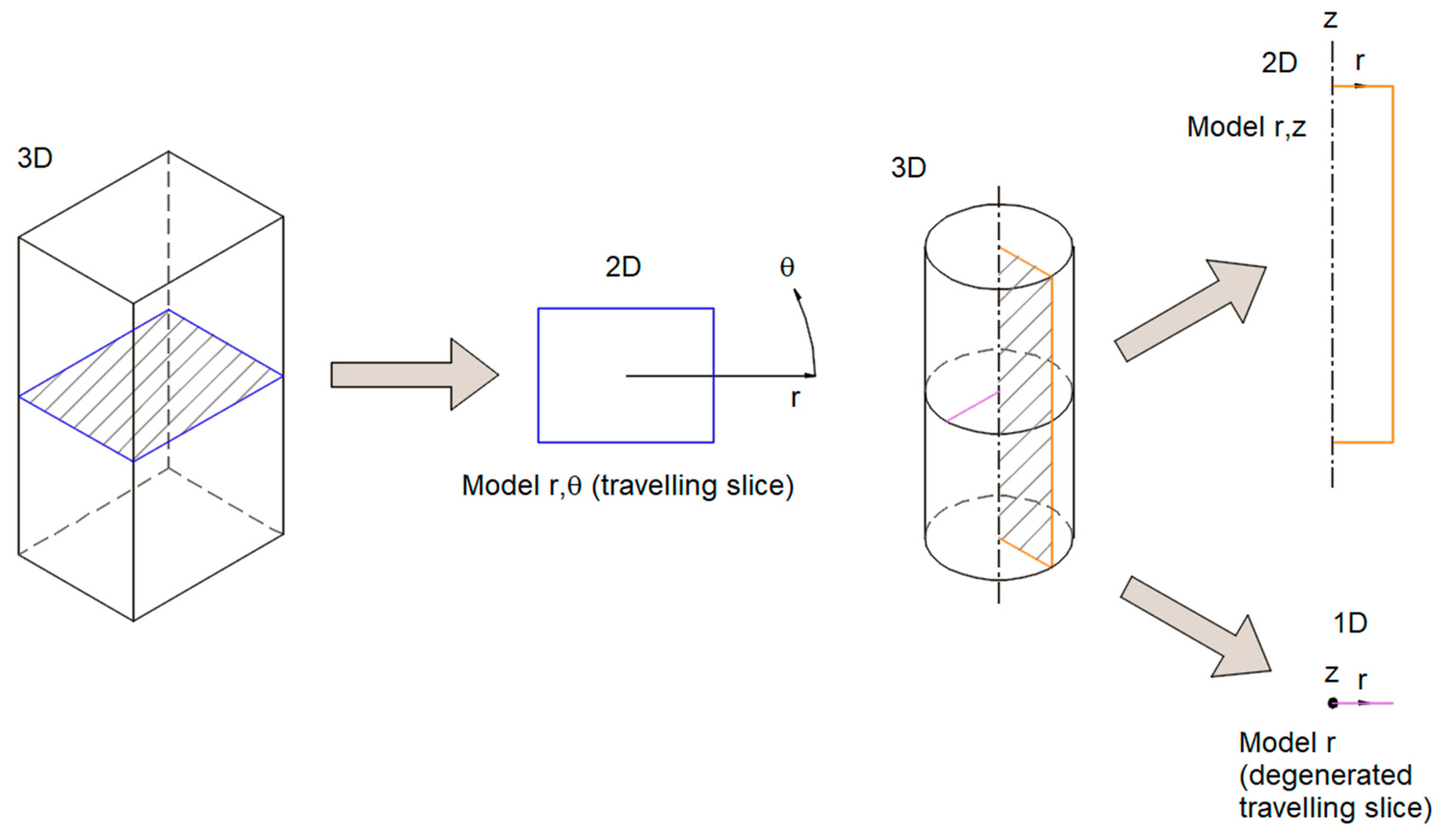
Due to the complexity of the phenomena that occur, the modeling of the steel continuous casting process must be multiphysics: thermal (solidification of molten metal, withdrawal of latent and sensible heat), mechanical (interaction between casted product and mould, friction, effect on the shape of pressure of the part which is still liquid), metallurgical (grain growth as a result of solidification, precipitation of secondary phases or carbides), and chemical (segregation of solutes, decomposition of lubricant). The fields stated above are interconnected and make the problem nonlinear; a common root for all of them is that they are temperature dependent. It must be noted that while the thermal problem can be tackled numerically with an almost feasible computational effort, this is not true when other fields, such as mechanical and metallurgical ones have to be taken into account; thus, a FE model reduced in dimensions should possibly be adopted. This article should be viewed as preparatory work of a certain modeling strategy that is intended to be used for offline calculations. The first step is to ensure its validity, beginning with the key aspect of the continuous casting process, the temperature distribution in the casted product, and then moving on with the other previously mentioned fields. Obviously, in the case of on-line calculation for process control purposes, a finite difference approach could be computationally more efficient at least for the thermal analysis. However, when casted profile becomes complex in shape (e.g., a beam blank in which both convex and concave zones are present), describing the boundary condition that a product is subjected to becomes challenging for finite differences models as well.
In a steel continuous casting plant (schematic representation of a continuous caster is given in Figure 1), the core equipment is represented by the mould, where in short time and small volume, compared to overall dimensions, a big amount of energy (order of magnitude: tens of MJ) is withdrawn from molten metal. This component is composed of copper due to its high thermal conductivity and is cooled by water. The thermal exchange between metal and mould is determined essentially by contact status; in early stages, when metal is too soft and not yet able to bear mechanical loads, the adherence and the withdrawal of energy are high. Moving downward stiffens the metal and creates a space between it and the mould, reducing thermal exchange and slowing the rate of growth of solidification of the shell. The solidified thickness at the mould exit must be sufficient to withstand the pressure imposed by the still-liquid inner metal.
As can be seen, heat exchange inside mould plays a significant role in the entire process; moreover, the majority of flaws on the casted material, such fractures and pinholes, are created here and are related to uneven heat extraction (see ref. [12]). It should be pointed out that uneven heat extraction results in irregular shell thickness growth for all casted sections: these phenomena are not predictable with a standard 3D FEM model, in which skin growth is kept as an average value. Other numerical models, i.e., CFD with RANS approaches, could address this issue, but are almost unfeasible for an industrial use due to long computational times.
What happens in the short space between the solidified shell and the mould surface is one of the most studied energy transfer mechanisms of the entire steel casting process; it can be represented by a thermal resistances model, in which each of them is the body (water, mould, lubricant, gap, shell, molten steel) crossed by heat. A comprehensive treatment can be found in ref. [13], while an interesting analysis on peak fluxes is given in ref. [14]. If each thermal resistance is known, starting from molten steel temperature all others in between and the thermal flux can be determined. This is the so-called fully coupled or direct approach, where both temperatures and flux are output; however, one of the difficulties of such modeling is to estimate the resistance value of the gap. Several studies on the gap creation in moulds have been carried out. Only in some specific circumstances, such as round shape, is the problem less complicated and a numerical approach can be used (see refs. [15,16]). For other common shapes such as squares (billet) and rectangles (bloom and slab), the computational cost for the gap estimation increases dramatically, necessitating a new approach: the problem decoupling. In the latter, once the thermal flux becomes an input, the complexity shifts onto the mathematical description of the heat withdrawn from the mould, which is dependent on several parameters such as casting speed, lubrication, material; e.g., for steel, two lubricants are typically used (powder or mineral oil) and specific grades (the peritectic ones) show differences in energy exchange (a quantification can be found in ref. [17]). To address this issue, mixed analytical-empirical models are used, see for example [18], so thermal flux is now established and no longer dependent from contact status; this is a strong assumption, but it allows the analysis to be performed in a reasonable amount of time. Typically, the mould flux trend decreases monotonically from meniscus to exit [13,18], although this statement in not widely accepted and a degree of uncertainty still remains.

3. Travelling Slice Model

3.1. Model Statement

As mentioned in the previous paragraph, the model has to take into account firstly the thermal aspect of continuous casting process. Analysis is transient and with temperature dependent thermal properties (taken from IDS software and then compared to [19] shows a very good agreement), and time/temperature dependent boundary conditions. In other words, Fourier’s equation shall be solved over the entire calculation domain:
H t = · ( λ T )
where T is temperature, H(T) is enthalpy, t is time, and λ is the thermal conductivity of metal that is casted. It should be noted that enthalpy is temperature dependent,. Following the physics of the steel continuous casting process, the model should be tridimensional. In fact, even though geometry remains constant in the casting direction (z axis), boundary conditions changes along z.
The most natural choice Is to use a growing mesh strategy, where new elements are added at domain during simulation; however, this approach is less often adopted due to a higher complexity. As mentioned before, a good computational alternative is to use a plane model (in the plane perpendicular to the z axis containing the product section), which moves in z direction according to the following law:
z t + Δ t = z t + v · Δ t
where t is time, Δt is time increment and v is casting speed. According to this approach, which is generally called travelling slice model, boundary conditions start below a certain level which can be chosen arbitrarily (e.g., 0), and casted products move in negative z direction; this means that all nodes above 0 shall have fixed temperatures in order to avoid thermal fluxes in the domain part, which has not yet been casted. As the nodes move below the aforementioned level, the fixed temperature condition disappears. For a generic non axisymmetric section, the alternative to a 3D model is a 2D travelling slice (also called r-θ model), see Figure 2. In the case of a casted round-shaped product, axisymmetry allows Equation (1) to be solved in a 2D model. In the latter case, the approximated travelling slice model degenerates into a 1D model (as visible in Figure 2).
This favorable circumstance allows a comparison of the two models (r-z and degenerated travelling slice) to be easily performed with less computational effort, which permits a parametric analysis to be carried out. It is thus possible to verify in a wide range of product dimensions and casting speeds the correctness of the hypothesis that heat conduction, namely energy transfer, in casting direction is negligible.

3.2. Boundary and Initial Conditions

In a steel continuous casting machine there are three different kinds of thermal exchange, each predominant in a certain part of it (as seen in Figure 3).
Thermal flux is withdrawn from the mould in order to start solidification; from a technical point of view, this is called primary cooling. When the mould is left, the casted product passes through a cooling chamber where energy is removed by arrays of water sprays (or air-mist for slabs). Here, two concurrent heat transfer mechanisms take place: convection with cooling media and radiation. The secondary cooling occurs in this zone. In the last part, machine cooling continues thanks to radiation only.
Since models are transient, an initial condition must be specified; this is a fixed temperature in all nodes of the calculation domain. For steel continuous casting, pouring temperature is the sum of liquidus temperature (which is dictated by chemical composition) and a specified superheat, namely the overheating relative to liquidus, typically in the range 20 ÷ 50 °C. This is done to avoid solidification in other devices (tundish and submerged entrance nozzle if present) prior to mould where steel shall remain in liquid phase, otherwise technological issues could halt or complicate the casting process.

3.2.1. Mould

As mentioned previously, thermal flux must be considered an input if a decoupled analysis is adopted, otherwise it becomes an output of the model; the first approach is employed in this research, as is done in the majority of published papers. From a global perspective, thermal flux acts on the domain borders; it is a Neumann’s boundary condition, expressed as follows:
q = λ T · n
where n is the unit vector perpendicular to surface and q is the thermal flux expressed in [W/m²].
From a mathematical point of view, the function above is one of time and coordinates (for shapes as billets, blooms and slabs):
q = f ( t i m e ,   c o o r d i n a t e s )
Thermal flux distributions are typically empiric: there are several references, however a first outlook can be found in [20,21].

3.2.2. Cooling Chamber

Cooling of the casted product that started in mould continues in this zone, where heat is withdrawn both by convection and radiation. A typical boundary condition could be written as
q = α T , c o o l i n g   f l o w   r a t e T s u r f T
where T s u r f is the surface temperature and T is the temperature outside the boundary layer. Temperature dependence is due to include radiation effects avoiding the fourth power exponent, simplifying its numerical treatment; for this reason, α can be considered an equivalent heat transfer coefficient. As for mould heat fluxes, several measuring tests have been conducted for heat transfer coefficients also, resulting in a wide range of empirical correlations (see refs. [20,21,22,23,24,25,26] for details).
The cooling chamber is divided into sectors that are fed with different water-flow rates; the first one is just after the mould, and connected to it is Sector 1 (also called “foot rolls”, in which cooling is intense), followed by Sector 2 (“mobile”) and then by other sectors (called “fixed”) until the end, depending on the machine layout and productivity. The three terms are enclosed in brackets because they refer to industrial jargon; for sake of clarity, the “mobile” sector does not move during casting its name comes from the fact that it is changed every time the cast section changes in order to get a more uniform cooling efficiency. The following sectors (the “fixed” ones) do not change because the cooling accuracy is less sensitive on the product quality when approaching the end of chamber. The longer the cooling chamber, the faster the casting pace (and thus productivity). The flow rate decreasing law is chosen to guarantee a smooth cooling path without excessive reheating on the product surface passing from a sector to the subsequent one. It shall be pointed out that the goal of secondary cooling is to achieve complete solidification prior to product cutting.

3.2.3. Cut to Length and Discharge

In this part, the casted product is not subjected to forced cooling anymore; it loses energy by radiation only. Hoods are used in some layouts to provide a passive control over how much temperature is left on the product prior to subsequent plastic deformation processes; in such cases, radiation losses are reduced in order to maintain a specified enthalpic level in it.

4. Case Study

Following the concepts shown until now, in the case of an axisymmetric product section, the plane model (or model r-z as in Figure 2) will be compared with the degenerated 1D travelling slice model. As mentioned previously, an increase of casted product size has been observed recently. It is therefore of great interest to analyze also these cases. For this purpose, three different casted shapes were investigated, including all rounds with diameters of 200 mm, 850 mm, and 1200 mm. The 200 mm round represents the traditional small-size product. Three casting speed values were created to vary in a range of industrial interest (from 2 m/min to 3 m/min). The 850 mm round represents a typical size of more a recent steelmaking plant used to feed the subsequent hot forging process. The adopted casting speed is 0.20 m/min. Nowadays, very big sections have been introduced as an alternative and more efficient process compared to ingot casting. The 1200 mm will be thus considered. Two values of casting speed are investigated: 0.08 m/min and 0.04 m/min; the latter one, although outside industrial range, has been considered to stress the travelling slice model to see if it fails.
All models have been implemented with commercial FE code MSC Marc and run on a 64-bit 8-processor (Intel(R) Core(TM) i7-8850H) with 64 GB installed RAM; Table 1 summarizes element and node counts. Degenerated travelling slice model adopts two node elements with linear interpolation along length (i.e., for Ø 200 mm, the radius is meshed with 100 linear elements, see Table 1); in these elements, heat can only flow along length. Model r-z, on the other hand, employs isoparametric four-node axisymmetric elements; in this case, the rectangular domain is discretized with a rather homogeneous mapping mesh, refined only towards the external radius to better simulate the high spatial temperature gradient associated with solidification. An automatic time stepping procedure has been selected for all simulation; equations are solved by using a multifrontal sparse solver in the framework of an implicit numerical scheme. More details can be found in [27].
Steel composition is given in Table 2, as well as its characteristics in Table 3; it shall be highlighted that during solidification, the latent heat is released uniformly in the range between solidus and liquidus temperatures (also known as the mushy zone). Thermal conductivity of the steel should be divided into two phases: for the liquid one the Wiedemann–Franz-Lorenz rule is employed, while for solid one regression, formulas from experimental measurements are followed; explanation of both approaches can be found in [19]. In Figure 4, the values of enthalpy and volumic mass are reported for different temperatures. Enthalpy trend is very similar to ref. [28]. This is a common structural steel, widely used for round bar, rebar, and beam production.
Boundary conditions are listed in Table 4, Table 5 and Table 6 for the three product diameters considered in this work. In particular, these indicate the thermal flux acting in mould, which is time dependent (the relation can be found in ref. [29]); since casting speed is constant during simulation, the dependence could be converted as position and thermal flux could be function of distance from meniscus. Moreover, the heat transfer coefficient (HTC) in the subsequent regions is reported; the latter one has been calculated according to ref. [20] and is speed dependent; for Ø 200 mm, examples in Table 4 reports the three HTCs values (respectively for 2 m/min, 2.5 m/min, and 3 m/min casting speed). For Ø 850 mm and Ø 1200 mm cases, a single HTC value is provided as only one casting speed has been considered. It must be observed that as a casted section increases, a less intense cooling is required due to lower casting speed and higher energy stored in the liquid steel. As pointed out previously, cooling is mainly governed by radiation in the discharge section.

5. Result and Discussion

Figure 5, Figure 6 and Figure 7 use normalized distance as the abscissa; this is the ratio between local distance and the position of cutting devices, which is located 35 m after meniscus in all cases. Figure 5 represents the computed temperatures (surface and core) for the three cases of Ø 200 mm; both surface and core temperature are given. A similar pattern for all speeds is visible, although with different values; moreover, it can be observed that the complete solidification is reached before for lower speed, which is completely consistent with plant operations and reference [30].
Figure 6 compares both models for Ø 850 mm casted at 0.20 m/min. The agreement between them is significant, since the two curves are virtually overlapped. In Table 7, the relative error for all sections and all casting speeds can be observed. The error is calculated as (Treference − Tapprox)/Treference, where subscript “reference” refers to model r-z while “approx” refers to degenerated travelling slice. The surface temperature is used as the reference temperature in all circumstances.
Please keep in mind that the comparison is limited to the two points that appear in all cases: mould exit and foot rolls (both of which appear in Table 4, Table 5 and Table 6). The relative error is far under the acceptable threshold for industrial use purposes.
Figure 7 relates to the biggest section, the Ø 1200 mm. It must be pointed out that casting speed in such case, namely 0.08 m/min, is close to the lowest operational limit in the continuous casting process. As stated in the previous paragraph, a case at 0.04 m/min has been done only with the purpose of investigating the applicability of the travelling slice model at very low casting speed; boundary conditions were different in the mould (average heat flux 316 kW/m²) but not in foot rolls, where same HTC (see Table 6) has been used. For this reason, the computed surface temperature results are low from an operational perspective. Moreover, it is visible that radial heat flux is always far bigger than axial one, confirming the correctness of neglecting this latter one (which is the fundamental hypothesis of travelling slice modeling). If this assumption is true for a such slow casted section, it will be even more so in the case of smaller and faster sections. Only in mould the radial thermal flux is imposed (with a descending law and its average value specified in Table 6), while it is the result of the computation in all other points; referring to Figure 7b, the dashed line is the imposed thermal flux, while the continuous one represents the calculated thermal flux (for both components).
Figure 8 shows the thermal field for Ø 1200 mm casted at 0.04 m/min, highlighting the “liquid pool end” that occurs, where the entire section has completely solidified (all domain is under solidus temperature).
It should be noted that travelling slice model yields the same metallurgical length of model bidimensional model, confirming its reliability in modeling the continuous casting process.
One of the last interesting aspects from a computational perspective, is the required time to run the models; it spans from 21 s to 123 s for a 1D degenerated travelling slice model (Ø 200 mm and Ø 1200 mm, respectively) to 22,285 s (Ø 200 mm) and 64,638 s (Ø 1200 mm) for model r-z.

6. Conclusions

In this work, the validity of the travelling slice model is investigated, notably in large dimension products and low casting speeds. Only in the case of a round section is a comparison with a reference model possible with a reasonable computational cost. Two different models (degenerated 1D travelling slice model and 2D axisymmetric reference model) have been developed and compared. The results show the validity of the travelling slice model in a wide range of product dimensions and casting speeds. Surface temperature comparison shows practically the overlap of profiles coming from both models with a relative error that is always less than 1.5%, also in case of the casting speed outside industrial range. Moreover, the component of thermal flux along casting direction is always a negligible portion of total flux, thus confirming the validity of the travelling slice model. It can be thus stated that also in case of big sections and low productivity, the travelling slice could be a reliable choice to model the continuous casting process. It should be highlighted that the computational cost of the reference 2D model is far higher the 1D approximated model; the ratio of calculation time for the same casted profile is proportional to 103, in favor of the travelling slice model (on the same hardware). In conclusion, it can be stated that the travelling slice approach could be considered a proven modeling technique in describing the continuous casting process. In future works, this will be extended to non-axisymmetric casted shapes, switching from 1D to 2D.

Author Contributions

Conceptualization, G.B.; methodology, G.B. and F.D.B.; validation, G.B.; formal analysis, G.B.; investigation, G.B. and F.D.B.; writing—original draft preparation, G.B.; writing—review and editing, F.D.B. All authors have read and agreed to the published version of the manuscript.

Funding

This research received no external funding.

Data Availability Statement

Restrictions are applied to the availability of the data used in this paper. Data were obtained from Danieli’s subsidiaries and are available upon request to Danieli & C. Officine Meccaniche spa.

Conflicts of Interest

G.B. declares to be an employee of Danieli & C. Officine Meccaniche SpA headquartered in Buttrio (Italy). F.D.B. declares no conflict of interest.

References

  1. Dong, Q.; Zhang, J.; Yin, Y.; Wang, B. Three-dimensional numerical modeling of macrosegregation in continuously cast billets. Metals 2017, 7, 209. [Google Scholar] [CrossRef]
  2. Yang, J.; Xie, Z.; Meng, H.; Hu, Z.; Liu, W.; Ji, Z. 3D transient heat transfer simulation and optimization for initial stage of steel continuous casting process. ISIJ Int. 2023, 63, 862–869. [Google Scholar] [CrossRef]
  3. Koric, S.; Abueidda, D. Deep learning sequence method in Multiphysics modeling of steel solidification. Metals 2021, 11, 494. [Google Scholar] [CrossRef]
  4. Han, H.N.; Lee, J.; Yeo, T.; Won, Y.M.; Kim, K.; Oh, K.H.; Yoon, J. A finite element model for 2-dimensional slice of cast strand. ISIJ Int. 1999, 39, 445–454. [Google Scholar] [CrossRef]
  5. Koric, S.; Thomas, B.G. Efficient thermo-mechanical model for solidification processes. Int. J. Numer. Meth. Engng. 2006, 66, 1955–1989. [Google Scholar] [CrossRef]
  6. Heger, J. Finite element modelling of mechanical phenomena connected to the technological process of continuous casting of steel. Acta Polytech. 2004, 44, 15–20. [Google Scholar] [CrossRef]
  7. Kong, Y.; Chen, D.; Liu, Q.; Long, M. A prediction model for internal cracks during slab continuous casting. Metals 2019, 9, 587. [Google Scholar] [CrossRef]
  8. Li, C.; Thomas, B.G. Thermo-mechanical finite element model of shell behavior in continuous casting of steel. In Proceedings of the Modeling of Casting, Welding and Advanced Solidification Processes X, San Destin, FL, USA, 25–30 May 2003; pp. 385–392. [Google Scholar]
  9. Nian, Y.; Zhang, L.; Zhang, C.; Ali, N.; Chu, J.; Li, J.; Liu, X. Application status and development trend of continuous casting reduction technology: A review. Processes 2022, 10, 2669. [Google Scholar] [CrossRef]
  10. Wang, E.; He, J. FE numerical simulation for influence of mold taper on thermomechanical behavior of steel billet in continuous casting process. J. Mater. Sci. Technol. 2001, 17 (Suppl. 1), s8–s12. [Google Scholar]
  11. Fang, Q.; Ni, H.; Zhang, H.; Wang, B.; Liu, C. Numerical study on solidification behavior and structure of continuously cast U71Mn steel. Metals 2017, 7, 483. [Google Scholar] [CrossRef]
  12. Kwon, S.H.; Won, Y.M.; Back, G.S.; Kim, H.; Lee, J.S.; Kim, D.G.; Heo, Y.U.; Yim, C.H. Prediction model for degree of solid-shell unevenness during initial solidification in the mold. ISIJ Int. 2021, 61, 2534–2539. [Google Scholar] [CrossRef]
  13. Saraswat, R.; Maijer, D.M.; Lee, P.D.; Mills, K.C. The effect of mould flux properties on thermo-mechanical behavior during billet continuous casting. ISIJ Int. 2007, 47, 95–104. [Google Scholar] [CrossRef]
  14. Mills, K.C.; Fox, A.B. The role of mould fluxes in continuous casting—So simple yet so complex. ISIJ Int. 2003, 43, 1479–1486. [Google Scholar] [CrossRef]
  15. Vynnycky, M. Air gaps in vertical continuous casting in round moulds. J. Eng. Math. 2010, 68, 129–152. [Google Scholar] [CrossRef]
  16. Vynnycky, M. Applied mathematical modelling of continuous casting process: A review. Metals 2018, 8, 928. [Google Scholar] [CrossRef]
  17. Jolivet, J.M.; Le Papillon, Y.; Bellavia, L. Development of high productivity casting of conventional and thin slabs. EUR 23887 Final Report. RFCS Publ. 2009. [Google Scholar] [CrossRef]
  18. Alizadeh, M.; Jahromi, A.J.; Abouali, O. New analytical model for local heat flux density in the mold in continuous casting of steel. Comput. Mater. Sci. 2008, 44, 807–812. [Google Scholar] [CrossRef]
  19. Mills, K.C.; Karagadde, S.; Lee, P.D.; Yuan, L.; Shahbzian, F. Calculation of physical properties for use in models of continuous casting processes—Part 2: Steels. ISIJ Int. 2016, 56, 274–281. [Google Scholar] [CrossRef]
  20. Cramb, A.W. The Making, Shaping and Treating of Steel (MSTS); The AISE Steel Foundation: Pittsburg, PA, USA, 2003. [Google Scholar]
  21. Assuncao, C.; Tavares, R.; Oliveira, G. Improvement in secondary cooling of continuos casting of round billets through analysis of heat flux distribution. Ironmak. Steelmak. 2015, 42, 1–8. [Google Scholar] [CrossRef]
  22. Wang, W.; Zhang, H.; Nakajima, K.; Lei, H.; Tang, G.; Wang, X.; Mu, W.; Jiang, M. Prediction of final solidification position in continuous casting bearing steel billets by slice moving method combined with Kobayashi approximation and considering MnS and Fe3P precipitation. ISIJ Int. 2021, 61, 2703–2714. [Google Scholar] [CrossRef]
  23. Long, M.; Chen, H.; Chen, D.; Yu, S.; Liang, B.; Duan, H. A combined hybrid 3-D/2-D model for flow solidification prediction during slab continuous casting. Metals 2018, 8, 182. [Google Scholar] [CrossRef]
  24. Milkowska-Piszczek, K.; Falkus, J. Control and design of the steel continuous casting process based on advanced numerical models. Metals 2018, 8, 581. [Google Scholar] [CrossRef]
  25. Li, L.; Zhang, Z.; Luo, M.; Li, B.; Lan, P.; Zhang, J. Control of shrinkage porosity and spot segregation in Ø195 mm continuously casted round bloom of oil pipe steel by soft reduction. Metals 2021, 11, 9. [Google Scholar] [CrossRef]
  26. Yang, J.; Ji, Z.; Liu, W.; Xie, Z. Digital-twin-based coordinated optimal control for steel continuous casting process. Metals 2023, 13, 816. [Google Scholar] [CrossRef]
  27. MSC Marc. Volume A: Theory and User Information; MSC Software Corporation: Irving, CA, USA, 2022. [Google Scholar]
  28. Ramirez-Lopez, A.; Davila-Maldonado, O.; Najera-Bastida, A.; Morales, R.D.; Rodriguez-Avila, J.; Muniz-Valdez, C.R. Analysis of non-symmetrical heat transfer during the casting of steel billets and slabs. Metals 2021, 11, 1380. [Google Scholar] [CrossRef]
  29. Cai, S.W.; Wang, T.M.; Xu, J.J.; Li, J.; Cao, Z.Q.; Li, T.J. Continuous casting novel mould for round steel billet optimized by solidification shrinkage simulation. Mater. Res. Innov. 2011, 15, 29–35. [Google Scholar] [CrossRef]
  30. Chen, Y.; Peng, Z.; Wu, L.; Zhao, L.; Wang, M.; Bao, Y. High-precision numerical simulation for effect of casting speed on solidification of 40Cr during continuous billet casting. Metall. Ital. 2015, 1, 47–51. [Google Scholar]
Figure 1. Sketch of a typical curved continuous casting machine. Molten steel in yellow, solidified steel in red. Cyan triangles: spray cooling.
Metals 13 01505 g001
Figure 2. Different modeling strategies.
Metals 13 01505 g002
Figure 3. Prevailing heat exchange mechanisms in a continuous casting machine.
Metals 13 01505 g003
Figure 4. Enthalpy and volumic mass trend for the selected steel.
Metals 13 01505 g004
Figure 5. Surface (a) and core (b) temperatures for Ø 200 mm.
Metals 13 01505 g005
Figure 6. Comparison of both models on surface temperature (casted section Ø 850 mm).
Metals 13 01505 g006
Figure 7. Surface temperature at different casting speeds (a) and thermal flux components at 0.04 m/min for Ø 1200 mm (b).
Metals 13 01505 g007
Figure 8. Thermal field in [°C] on whole domain (top) and particular of “liquid pool end” (bottom) for Ø 1200 mm.
Metals 13 01505 g008
Table 1. Characteristics of FE models.
CaseDegenerated 1D Travelling SliceModel r-z
ElementsNodesElementsNodes
Ø 200 mm10010167,75670,389
Ø 850 mm425426117,270119,922
Ø 1200 mm600601138,118140,778
Table 2. Steel chemical composition.
ElementConcentration [%]ElementConcentration [%]
C0.210Mn1.500
Cr0.020Ni0.020
Mo0.002Si0.200
Cu0.035Al0.045
P0.010S0.002
V0.003FeBalance
Table 3. Some physical parameters of selected steel.
ParameterValue
Liquidus temperature1541 °C
Solidus temperature1457 °C
Solidification range84 °C
Latent heat297.66 kJ/kg
Table 4. Detail of applied boundary conditions for each zone for both models (cast section Ø 200).
ZoneLength [m]Boundary Condition
Mould (steel level)0.68Thermal flux according to [29]
Sect. 1 (Foot rolls)0.35HTC = 1410, 1489, 1523 W/m²·K (depending on speed)
Sect. 2 (Mobile)1.90HTC = 720, 759, 795 W/m²·K (depending on speed)
Sect. 3 (Fixed 1)2.30HTC = 320, 351, 390 W/m²·K (depending on speed)
Sect. 4 (Fixed 2)1.15HTC = 269, 280, 309 W/m²·K (depending on speed)
Discharge28.6Radiation to environment
Table 5. Detail of applied boundary conditions for each zone for both models (cast section Ø 850).
ZoneLength [m]Boundary Condition
Mould (steel level)0.64Average thermal flux = 548 kW/m²
Sect. 1 (Foot rolls)0.40HTC = 331 W/m²·K
Sect. 2 (Mobile 1)0.75HTC = 251 W/m²·K
Sect. 3 (Mobile 2)0.75HTC = 242 W/m²·K
Discharge32.46Radiation to environment
Table 6. Detail of applied boundary conditions for each zone for both models (cast section Ø 1200).
ZoneLength [m]Boundary Condition
Mould (steel level)0.64Average thermal flux = 413 kW/m²
Sect. 1 (Foot rolls)0.40HTC = 296 W/m²·K
Discharge33.96Radiation to environment
Table 7. Relative error on the computed surface temperature for all studied cases in two points.
CaseMould ExitFoot Rolls
Ø 200 mm–2.00 m/min0.19%−0.74%
Ø 200 mm–2.50 m/min0.19%0.51%
Ø 200 mm–3.00 m/min0.28%−0.59%
Ø 850 mm–0.20 m/min0.09%−0.28%
Ø 1200 mm–0.08 m/min0.20%0.43%
Ø 1200 mm–0.04 m/min−0.87%1.15%
Disclaimer/Publisher’s Note: The statements, opinions and data contained in all publications are solely those of the individual author(s) and contributor(s) and not of MDPI and/or the editor(s). MDPI and/or the editor(s) disclaim responsibility for any injury to people or property resulting from any ideas, methods, instructions or products referred to in the content.

