Numerical Simulation of Flow Field, Bubble Distribution and Solidified Shell in Slab Mold under Different EMBr Conditions Assisted with High-Temperature Quantitative Velocity Measurement

Abstract

The flow field, bubble distribution and solidified shell in slab mold are numerically simulated with large eddy simulation (LES) under different electromagnetic braking (EMBr) conditions, assisted with high-temperature quantitative velocity measurement. The calculated velocities on the mold surface are in good agreement with the measured values of the industrial experiment at high temperature with the rod deflection method under different EMBr conditions and different argon flow rates, which verifies the correctness of the model. After EMBr is applied, the flow velocity on the surface of the mold decreases. With EMBr, the velocity on the mold surface first increases and then decreases with the increase in argon flow rate. When the argon flow rate is 10 L·min⁻¹, the jets at the side ports of the submerged entry nozzle (SEN) become disordered, and the liquid level fluctuation near the SEN wall intensifies, which increases the risk of slag entrainment and slag layer breaking and the risk of argon bubbles being captured. When the argon flow rate is 6 L·min⁻¹, the velocity and fluctuation on the mold surface can be significantly reduced by use of double-ruler EMBr; the impact of the jet on the narrow face of the mold is obviously restrained; and the solidified shell thickness increases.

1. Introduction

The automobile exposed panel has extremely strict requirements for surface quality, and reducing the incidence of surface defects is very important for many steelmaking plants in the world. The production of hot-dip galvanized automobile exposed panel is a complex long process, including the steelmaking process of hot metal pretreatment, converter blowing, secondary refining and continuous casting, as well as the post processes, such as hot rolling, pickling, cold rolling, continuous annealing and hot-dip galvanizing processes. Most of the surface defects, such as inclusion defect, gas bubble defect and mold flux entrainment defect, are formed in the continuous casting process, especially in the mold. Therefore, the surface defects caused in steelmaking process are closely related to the flow field in the mold. The inappropriate flow field in the mold, such as large liquid level fluctuation, too fast surface velocity and single-roll flow pattern, tends to lead to the entrapment of mold flux particles, argon bubbles and inclusions, which may be captured by the primary solidified shell to form the surface defects on the automobile exposed panel [1,2,3,4,5]. Therefore, optimizing the mold flow field has become an important method to improve the quality of the continuous casting slab for producing the automobile exposed panel.

The entrapment of mold flux is usually one of the most common defects, which is closely related to the surface velocity in the mold. An excessively large surface velocity will seriously fluctuate the interface of the molten steel and mold flux, probably resulting in the emulsification of the mold flux and entrapment of the mold flux into the molten steel [6,7]. Zhang et al. [6] indicated that when the chemical reactions at the interface of steel and slag are not considered, the critical molten steel speed on the mold surface for slag entrainment is 0.463–0.541 m·s⁻¹. When considering the decrease in slag viscosity caused by the chemical reactions at the interface of steel and slag, the critical speed for slag entrainment decreases to 0.29 m·s⁻¹. Adjusting the continuous casting process parameters can significantly change the velocity on the mold surface. When the casting speed is increased, the velocity and fluctuation on the mold surface increase significantly, resulting in the mold flux being more easily entrapped into the molten steel to form mold flux defects [8]. Chen et al. [9] studied the flow field in the slab mold under different argon flow rates, showing that with the increase in argon flow rate, the flow pattern in the mold changes from double-roll flow to single-roll flow. The surface velocity and fluctuation become great near the submerged entry nozzle (SEN), which is prone to slag entrapment. Generally, the optimization of the flow field in the mold can be realized with adjusting the relevant continuous casting process parameters, such as casting speed, argon flow rate, SEN immersion depth and SEN structure, to some extent.

Although the conventional optimization of continuous casting process parameters can partially improve the mold flow field, it still cannot meet the increasingly strict requirements for high surface quality for automobile exposed panel, especially under the condition of high casting speed. Therefore, electromagnetic braking (EMBr) is employed to control the mold flow field because of its advantages of non-contact and easy adjustment of process parameters. At present, slab EMBr devices are mainly divided into three categories: local, single-ruler and double-ruler EMBr. For local EMBr, the static magnetic field is arranged near the side port of SEN to reduce the jet velocity of molten steel [10,11]. For single-ruler EMBr, the static magnetic field is arranged below the SEN, which can reduce the jet velocity and inhibit the lower circulating flow [12,13]. For double-ruler EMBr, a pair of magnetic poles is installed near the meniscus on the basis of the single-ruler EMBr. It not only has the advantage of single-ruler EMBr in reducing the jet velocity, but it can also reduce the velocity on the surface of the mold and prevent the entrapment of the mold flux into the molten steel [14,15].

In recent years, for the application of EMBr in slab mold, the influence of continuous casting process parameters on the flow field in the mold has been studied [16,17,18,19,20,21,22]. Liu et al. [16] studied the flow pattern of the mold under the condition of single-ruler and double-ruler EMBr. The results show that under the condition of single-ruler EMBr, the lower circulation flow in the mold is the piston flow, being significantly inhibited. Under the condition of double-ruler EMBr, the lower circulating flow is also suppressed, and the velocity and fluctuation on the mold surface are significantly reduced as well. Sarkar et al. [17] studied the mold flow field with different argon flow rates under the condition of EMBr and found that although the fluctuation near the meniscus increases with the increase in argon flow rate, EMBr can inhibit the fluctuation of the mold surface caused by argon to some extent. Yin et al. [18] studied the movement of argon bubbles and inclusions in the mold of double-ruler EMBr and found that EMBr weakens the movement of inclusions in the mold and reduces the number of inclusions on the surface of the slab, but it increases the number of inclusions in the slab interior. In addition to the study of continuous casting process parameters, Yin et al. [23] also studied the slag entrainment mechanism under EMBr. When there is no argon gas injection, three kinds of slag entrainment mechanisms are found: shear flow, Von Kármán vortex and liquid level fluctuation. When there is an argon injection, a new slag entrainment mechanism will appear: bubble interaction, which is the main slag entrainment mechanism under the conditions of EMBr and argon injection.

Some research works have been conducted on the flow field, temperature field and particle motion in the slab mold under the condition of EMBr. However, on the one hand, no comparison was made between the calculation results and the quantitative high-temperature measurement results of flow velocity on the surface of the mold. On the other hand, the influence of solidified shell was rarely considered in the numerical calculation. In our previous works, the mold surface velocity was measured using the rod deflection method [24] and was compared with the numerical simulation results. The flow fields in the slab mold with the narrow width [25], wide width [26] and medium width [27] were studied with numerical simulation and high-temperature velocity measurement near the mold surface. The influence of the mold flux and the solidified shell [28] on the mold flow field in the mold were further investigated.

Therefore, in the present work, the industrial experiments of quantitative measurement of mold surface velocity at high temperature were carried out, and the magnetic field distribution in the mold was also measured. Then, under the condition of EMBr and considering the influence of the solidified shell and mold flux, the numerical simulation calculation was carried out through large eddy simulation (LES) + volume of fluid (VOF) + discrete phase model (DPM), and the calculation results were compared with the quantitative measurement results to verify the correctness of the model. Furthermore, the flow field in the slab mold, the fluctuation on the mold surface, the thickness of the solidified shell and the distribution of argon bubbles were numerically simulated.

2. Mathematical Model

2.1. Assumptions

With regard to the complex transfer phenomenon in the mold, the following reasonable assumptions are made to simplify the numerical calculation of the flow field:

(1)

Liquid steel and mold flux are incompressible Newtonian fluids;

(2)

Liquid steel and mold flux in the mold are in the homogeneous phase, and parameters such as density and viscosity are set to be constants;

(3)

The influence of mold oscillation and taper is not considered;

(4)

The shape of argon bubbles is spherical, ignoring the breakage and coalescence of argon bubbles;

(5)

The influence of Joule heat generated by electric currents is ignored;

(6)

The molten steel in the paste zone obeys Darcy’s law;

(7)

The influence of liquid steel flow on the electromagnetic field is ignored.

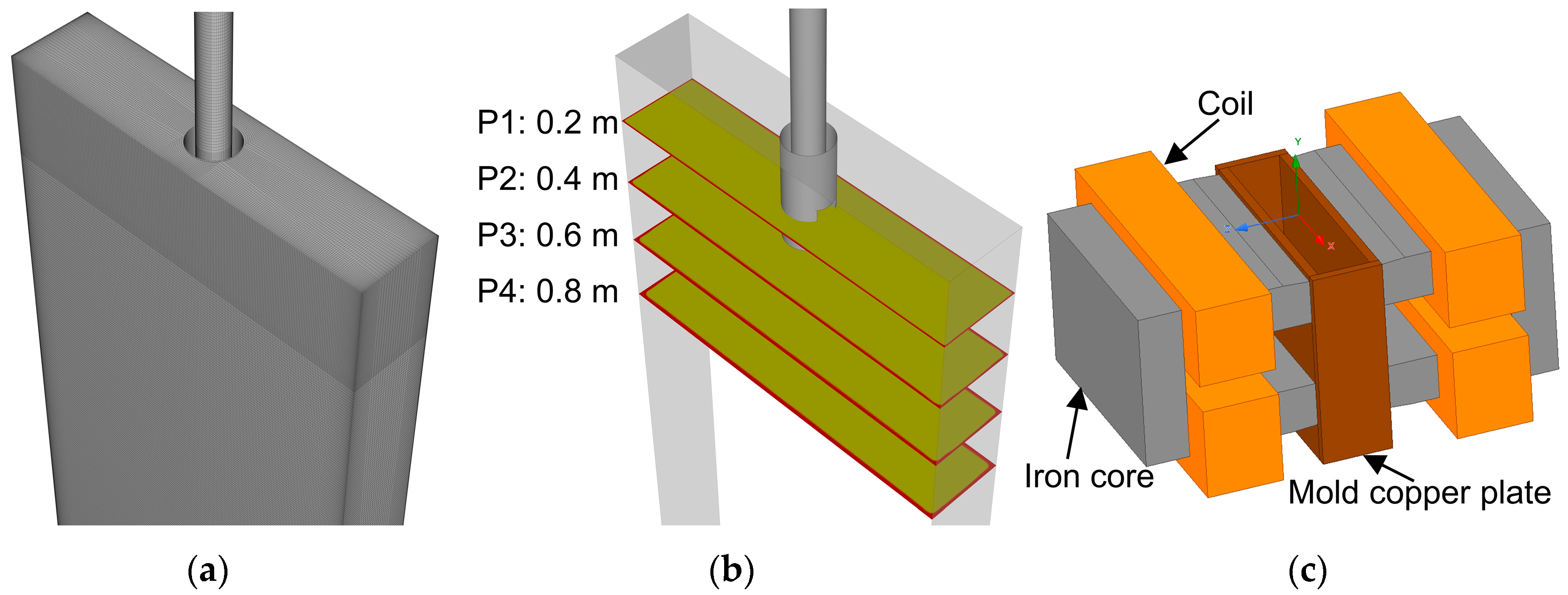
2.2. Electromagnetic Force Model

The Lorentz force is calculated with the electric potential method [29]. The electric current $\overrightarrow{J}$ can be obtained with Equation (1), and the conservation of the electric current is given by Equation (2):

$$\overrightarrow{J}=\sigma (\overrightarrow{E}+{\overrightarrow{u}}_1\times {\overrightarrow{B}}_0)=\sigma (-\nabla \varphi +{\overrightarrow{u}}_1\times {\overrightarrow{B}}_0)$$

(1)

$$\nabla \cdot \overrightarrow{J}=0$$

(2)

The electric potential $\varphi$ is solved as follows:

$$\nabla \cdot (\nabla \varphi )=\nabla \cdot ({\overrightarrow{u}}_1\times {\overrightarrow{B}}_0)$$

(3)

The Lorentz force ${\overrightarrow{F}}_{\mathrm{Lorentz}}$ is given by

$${\overrightarrow{F}}_{\mathrm{Lorentz}}=\overrightarrow{J}\times {\overrightarrow{B}}_0$$

(4)

where $\sigma$ is the electrical conductivity, $\overrightarrow{E}$ is electric field intensity, ${\overrightarrow{B}}_0$ is magnetic flux density, and ${\overrightarrow{u}}_1$ is liquid steel velocity.

2.3. Discrete Phase Model

The argon bubble is regarded as a discrete phase, and the motion trajectory of the argon bubble is calculated through the DPM model. The balance equation of force on each argon bubble is as follows:

$${\rho }_{\mathrm{p}}\frac{\pi }{6}{d}_{\mathrm{p}}^3\frac{\mathrm{d}{\overrightarrow{u}}_{\mathrm{p}}}{\mathrm{d}t}={\overrightarrow{F}}_{\mathrm{D}}+{\overrightarrow{F}}_{\mathrm{p}}+{\overrightarrow{F}}_{\mathrm{b}}+{\overrightarrow{F}}_{\mathrm{VM}}+{\overrightarrow{F}}_1$$

(5)

The relevant force on the right of the equation refers to the relevant previous work [16]. ${\rho }_{\mathrm{p}}$ is argon bubble density, $d_{\mathrm{p}}$ is argon bubble diameter, ${\overrightarrow{u}}_{\mathrm{p}}$ is argon bubble velocity, ${\overrightarrow{F}}_{\mathrm{D}}$ is the drag force, ${\overrightarrow{F}}_{\mathrm{p}}$ is the pressure gradient force, ${\overrightarrow{F}}_{\mathrm{b}}$ is the buoyancy force, ${\overrightarrow{F}}_{\mathrm{VM}}$ is the virtual mass force and ${\overrightarrow{F}}_1$ is the lift force.

The drag force can be given as follows:

$${\overrightarrow{F}}_{\mathrm{D}}=\frac{\pi }{8}{d}_{\mathrm{p}}^2{C}_{\mathrm{D}}{\rho }_1\left|{\overrightarrow{u}}_{\mathrm{p}}-{\overrightarrow{u}}_1\right|\left({\overrightarrow{u}}_{\mathrm{p}}-{\overrightarrow{u}}_1\right)$$

(6)

where ${\rho }_1$ is the density of molten steel, $C_{\mathrm{D}}$ is the dimensionless drag coefficient related to the Reynolds number of argon bubbles, whose specific expression is

$$C_{\mathrm{D}}=\frac{24}{{\mathrm{Re}}_{\mathrm{p}}}\left(1+0.15{\mathrm{Re}}_{\mathrm{p}}^{0.687}\right)$$

(7)

where ${\mathrm{Re}}_{\mathrm{p}}$ is the Reynolds number of argon bubble, and the specific expression is ${\mathrm{Re}}_{\mathrm{p}}=d_{\mathrm{p}}\left|{\overrightarrow{u}}_{\mathrm{p}}-{\overrightarrow{u}}_1\right|/v$. $v$ is the viscosity of liquid steel.

The pressure gradient force can be expressed as

$${\overrightarrow{F}}_{\mathrm{p}}=-\frac{\pi }{6}{d}_{\mathrm{p}}^3\nabla p$$

(8)

The expression of the buoyancy force is

$${\overrightarrow{F}}_{\mathrm{b}}=\frac{\pi }{6}{d}_{\mathrm{p}}^3\left({\rho }_1-{\rho }_{\mathrm{p}}\right)\overrightarrow{g}$$

(9)

The expression of the virtual mass force is

$${\overrightarrow{F}}_{\mathrm{VM}}=\frac{\pi }{6}{d}_{\mathrm{p}}^3{\rho }_1{C}_{\mathrm{VM}}\frac{d}{dt}\left({\overrightarrow{u}}_1-{\overrightarrow{u}}_{\mathrm{p}}\right)$$

(10)

where $C_{\mathrm{VM}}$ is the virtual mass force coefficient, which is set to be 0.5.

The lift force can be described as

$${\overrightarrow{F}}_1=1.62d_{\mathrm{p}}^2{\left({\rho }_1{\mu }_{eff}\right)}^{1/2}{\left|\nabla \times {\overrightarrow{u}}_1\right|}^{-1/2}\left(\left({\overrightarrow{u}}_1-{\overrightarrow{u}}_{\mathrm{p}}\right)\times \left(\nabla \times {\overrightarrow{u}}_1\right)\right)$$

(11)

2.4. Multiphase Flow Model

The influence of liquid slag layer on the mold flow field is taken into consideration. The VOF model can simulate two or more fluid phases [30]. At present, it is used to simulate the interface of steel and slag. By solving the volume fraction of continuity equation, the interface between the phases can be tracked:

$$\frac{1}{{\rho }_i}\left[\frac{\partial }{\partial t}\left({\rho }_i{\alpha }_i\right)+\nabla \cdot \left({\rho }_i\overrightarrow{u}{\alpha }_i\right)\right]=0$$

(12)

$$\sum _{i=1}^n{\alpha }_i=1$$

(13)

where ${\alpha }_i$ is the volume fraction of the $i_{\mathrm{th}}$ phase, and $p_i$ is the density of the $i_{\mathrm{th}}$ phase.

When using the VOF model, each phase shares the velocity field and solves a single momentum equation in the whole calculation domain. The momentum equation is as follows:

$$\frac{\partial }{\partial t}(\rho \overrightarrow{u})+\nabla \cdot (\rho \overrightarrow{u}\overrightarrow{u})=-\nabla p+\nabla \cdot \left[\mu \left(\nabla \overrightarrow{u}+\nabla {\overrightarrow{u}}^T\right)\right]+\rho \overrightarrow{g}+{\overrightarrow{F}}_{\text{bubble}}+{\overrightarrow{F}}_{\sigma }+{\overrightarrow{F}}_{\mathrm{Lorentz}}$$

(14)

where $p$ is the pressure, $\overrightarrow{g}$ is the gravitational acceleration, ${\overrightarrow{F}}_{\mathrm{bubble}}$ is the momentum transfer term exerted by the discrete bubbles, and ${\overrightarrow{F}}_{\sigma }$ is the surface tension at the interface. Density $\rho$ and viscosity $\mu$ are determined by the properties of each phase:

$$\rho =\sum _{i=1}^n{\rho }_i{\alpha }_i,\mu =\sum _{i=1}^n{\mu }_i{\alpha }_i$$

(15)

2.5. Large Eddy Simulation and Solidification

The turbulence model used in this paper is the WMLES S-Omega model [31]. In the WMLES S-Omega model, the eddy viscosity $v_t$ is calculated as follows:

$$v_t=\min \left[{\left(\kappa d_w\right)}^2,{\left(C_{Smag}\Delta \right)}^2\right]\cdot |S-\Omega |\cdot \left\{1-\exp \left[-{\left(y^{+}/25\right)}^3\right]\right\}$$

(16)

where $d_w$ is the wall distance, $S$ is the strain rate, $\Omega$ is the vorticity magnitude, $\kappa =0.4187$, $C_{Smag }=0.2$, $y^{+}$ is the normal to the wall inner scaling. The LES model is based on a modified grid scale to account for the grid anisotropies in wall-modeled flows:

$$\Delta =\min \left(\max \left(C_w\cdot d_w,C_w\cdot h_{\max },h_{wn}\right);h_{\max }\right)$$

(17)

where $h_{\max }$ is the maximum edge length of the hexahedral grid, $h_{wn}$ is the normal grid spacing of the wall, and $C_w=0.15$.

As mentioned in the basic assumptions above, the solidification of molten steel obeys Darcy’s law. The molten steel between the solidus and liquidus is regarded as a porous medium, and the source terms are applied to the fluids. When the temperature of molten steel changes, the porosity and source term also change. The formula is as follows:

$$\beta =\{\begin{array}{cc}0& T\le T_{\text{solidus}}\\ \frac{T-T_{\text{solidus}}}{T_{\text{liquidus}}-T_{\text{solidus}}}& T_{\text{solidus}}\le T\le T_{\text{liquidus}}\\ 1& T\ge T_{\text{liquidus}}\end{array}$$

(18)

$$S=\frac{{(1-\beta )}^2}{\left({\beta }^3+\xi \right)}{A}_{\text{mush}}\left(\overrightarrow{u_1}-\overrightarrow{u_c}\right)$$

(19)

where $\beta$ is the volume fraction of liquid steel, $T_{\mathrm{solidus}}$ is the solidus temperature of steel, $T_{\text{liquidus}}$ is the liquidus temperature of steel, $\xi$ is a very small number to prevent division by zero, $A_{\text{mush}}$ is the mushy zone constant, $\overrightarrow{u_{\mathrm{c}}}$ is the casting speed, and details regarding the solidification calculation can be referred to in our previous work [32].

2.6. Numerical-Simulation-Related Calculation Parameters

Figure 1a is a schematic diagram of the mold grid. The hexahedrally structured grid is used in the whole calculation domain. In order to improve the simulation accuracy of the interface of steel and slag and the solidified shell, the grids in the slag layer and near the wide face and narrow face of the mold are densified, and the total number of grids is about 1.65 million.

Table 1. Continuous casting parameters and material physical parameters.

Parameters	Values	Parameters	Values
Mold width (mm)	1050	Slag thickness (mm)	15
Mold thickness (mm)	230	Slag density (kg·m−3)	2800
Mold length (mm)	800	Slag viscosity (kg·m−1·s−1)	0.18
SEN submergence depth (mm)	170	Liquidus temperature (K)	1807
SEN port angle (°)	20	Solidus temperature (K)	1796
SEN port size (mm × mm)	70 × 90	Thermal conductivity (W·m−1·K−1)	34
SEN inner diameter (mm)	78	Steel latent heat (J·kg−1)	270,000
SEN outer diameter (mm)	140	Steel electric conductivity (S·m−1)	580,000
Argon flow rate (L·min−1)	0\6\10	Steel magnetic conductivity (H·m−1)	1.257 × 10−6
Argon density (kg·m−3)	0.4	Steel viscosity (kg·m−1·s−1)	0.0062
Steel density (kg·m−3)	7020	Casting speed (m·min−1)	1.9

lists the physical parameters of relevant materials and relevant continuous casting process parameters. For the size distribution of argon bubbles, according to the results of our water model experiment and through proportional conversion, the size of the argon bubbles follows the Rosin–Rammler distribution. The diameter range of the argon bubbles is from 2.0 mm to 6.0 mm. In order to investigate the flow field in the mold and the change in the solidified shell, four reference planes with the depth from the meniscus within 0.8 m are selected. As shown in Figure 1b, the distances between the reference planes P1, P2, P3 and P4 and the liquid level of the mold are 0.2, 0.4, 0.6 and 0.8 m, respectively. Figure 1c shows the schematic diagram of a double-ruler EMBr device, mainly including coil, iron core and mold copper plate.

The inlet of the SEN is a velocity inlet boundary condition, and the outlet of the mold is a pressure outlet boundary condition. The mold surface is considered a free slip and fix. The wide and narrow surfaces are non-slip and stationary. The argon bubbles are injected from the inlet of SEN and escape from the surface of the mold. The SEN and its wall are reflection conditions, and the wide and narrow surface of the mold are trap conditions.

In this paper, the ANSYS ICEM 2021 R1 is used to establish the grid, and ANSYS Fluent 2021 R1 is used for calculation and post-processing. For the calculation of EMBr, firstly, the ANSYS Maxwell 2021 R1 is used to calculate the relevant EMBr parameters and export the MAG file. Then, Fluent activates the MagnetoHydroDynamic (MHD) module and imports the MAG file to calculate the fluid field with EMBr. In the overall calculation process, the Reynolds-averaged Navier–Stokes (RANS) method is firstly used to calculate the steady-state flow field, and then, the unsteady conditions are activated. At the same time, the MHD module, DPM model, LES, energy equation and solidification and melting model are open. After the calculation is stable, the average data within 10 s are taken as the time average result.

Three EMBr conditions with argon flow rate of 6 L·min⁻¹ are studied, which are referred to as Mode 1, Mode 2 and Mode 3. Mode 1 is where the upper and lower coils are not powered on, and there is no EMBr; Mode 2 has the upper coil current 0 A and lower coil current 700 A. In Mode 3, the upper coil current is 300 A, and the lower coil current is 700 A. In addition, the effects of three argon flow rates of 0, 6 and 10 L·min⁻¹ on the mold flow field with EMBr Mode 3 are also studied.

3. Results and Discussion

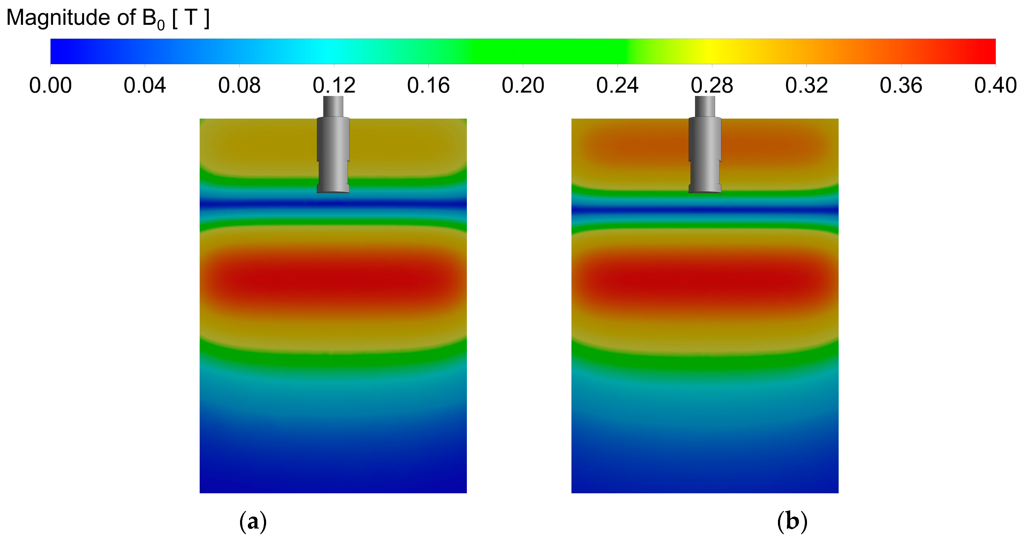
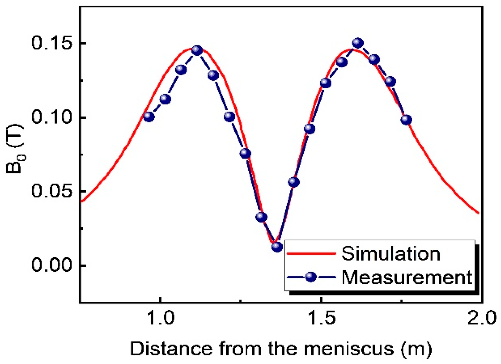
3.1. Magnetic Flux Density Distribution and Model Verification

Figure 2 shows the numerical results of the magnetic flux density distribution in the mold under the conditions of EMBr in Mode 2 and Mode 3. The center of the upper coil is above the SEN, and the center of the lower coil is below the SEN. As can be seen from Figure 2a, under the condition of Mode 2, the magnetic flux density distribution is mainly distributed below the SEN. Due to the magnetic conduction of the iron core, there is a weak magnetic flux density above the SEN. The magnetic field interaction leads to a region with zero magnetic flux density below the SEN. According to Figure 2b, under the condition of Mode 3, the magnetic flux density is mainly distributed in the upper and lower parts of the SEN. Compared with Mode 2, the magnetic flux density near and above the SEN is enhanced due to the energization of the upper coil, resulting in the downward shift of the area with zero magnetic flux density.

In order to verify the correctness of the numerical results of magnetic flux density distribution in the mold, the numerical results and experimental measurement results of magnetic flux density distribution in the slab mold of a steelmaking plant are compared. The magnetic flux density is measured on the central axis of the mold along the longitudinal direction. Figure 3 gives the comparison between the numerical results and the actual measurement results of the magnetic flux density distribution at the transverse center of the mold when the upper coil current is 200 A, and the lower coil current is 200 A. It can be seen that the calculation results are in good agreement with the experimental results.

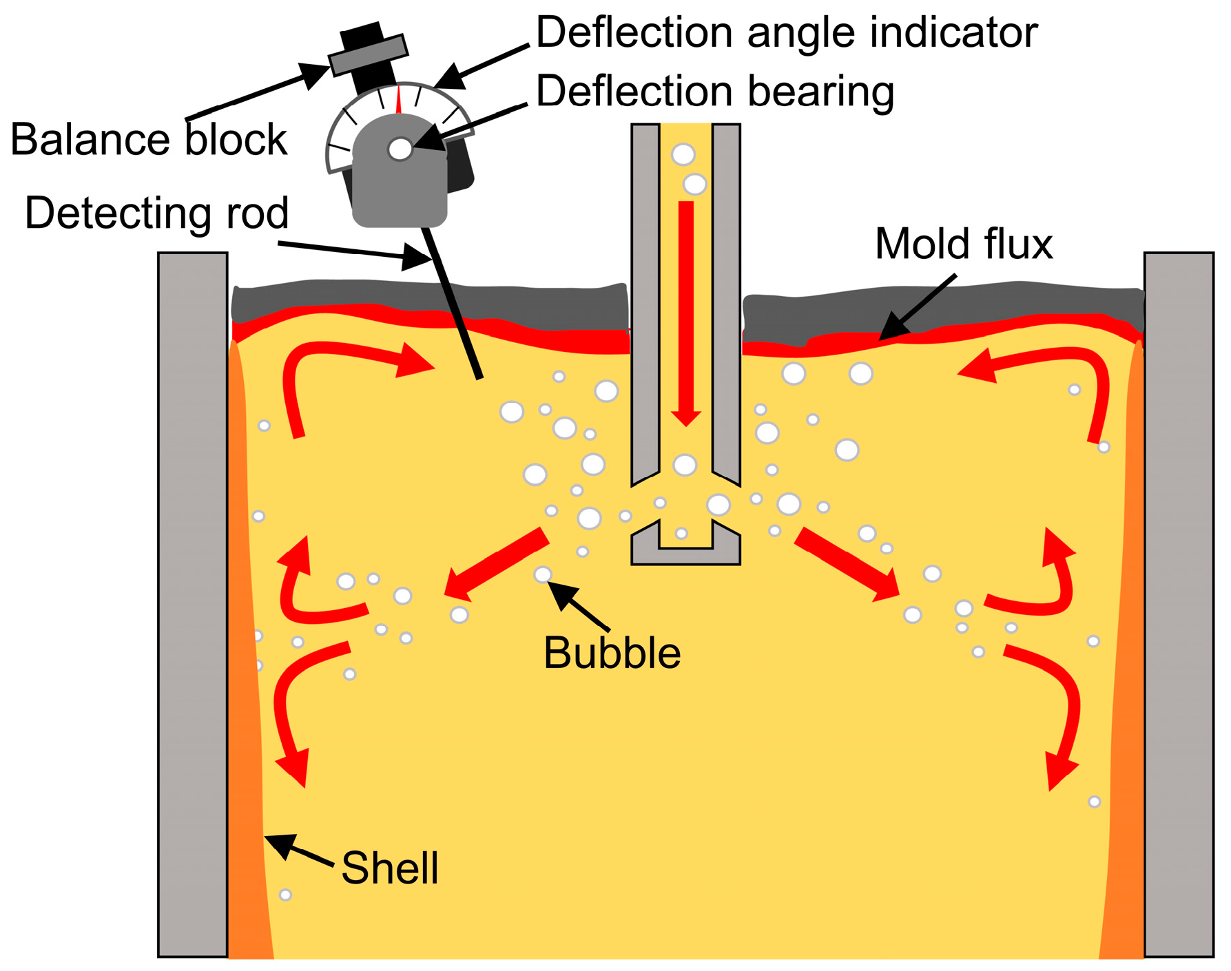
3.2. Comparison between the Calculated and Measured Velocities near the Mold Surface

In our previous works, the method for quantitative measurement of the velocity near the mold surface at high temperature, named the rod deflection method, was developed [24,25]. Figure 4 is a schematic diagram of the rod deflection method. The velocity measuring device is composed of a detecting rod, a deflection bearing, a deflection angle indicator and a balance block. After the detecting rod is inserted into the liquid steel, the detecting rod deflects under the impact of the liquid steel flow. After the deflection angle indicator is stable, the deflection angle is read, and the liquid steel velocity near the mold surface can be obtained through the relationship between the deflection angle and the liquid steel velocity. The velocity near the surface of one-quarter width of the mold is measured with the rod deflection method.

Figure 5 is the comparison of the calculated and measured velocities of molten steel near the mold surface under the different argon flow rates in the EMBr Mode 3. The compared velocities are the values at the one-quarter width position of the thickness center slice of the mold. Under different argon flow rates, the calculated velocities on the mold surface are in good agreement with the measured values of the industrial experiment with the rod deflection method. With the increase in argon flow rate, both of the calculated and measured velocities first increase and then decrease.

Figure 6 gives the comparison of the calculated and measured velocities of molten steel on the mold surface under the different EMBr modes and at the argon flow of 6 L·min⁻¹. As the EMBr mode changes from Mode 1 to Mode 2 and then to Mode 3, both of the calculated and measured velocities of liquid steel on the mold surface gradually decrease. However, the calculated values are slightly lower than the measured ones, which may be due to the overestimation of the applied magnetic field in the mold by using the vacuum permeability in the numerical simulation.

As shown in Figure 5, under the condition of no argon injection and EMBr Mode 3, the velocity at one-quarter width of the mold is too low, which is not conducive to the melting of the mold flux. When the argon flow rate is increased to 6 L·min⁻¹, the appropriate argon flow rate plays a role in activating the surface flow of the mold. The surface velocity increases to about 0.20 m·s⁻¹, which can optimize the heat and mass transfer conditions near the meniscus. When the argon flow rate is further increased to 10 L·min⁻¹, affected by the upward floating of argon bubbles, the jet velocity and penetration depth of liquid steel at the side ports of the SEN are significantly reduced; the upward circulating flow is strongly disturbed by the upward floating of more argon bubbles, thus, the surface velocity of the mold is reduced. According to the calculation results in Figure 5b, when the argon flow rates are 6 L·min⁻¹ and 10 L·min⁻¹, the maximum values of the surface velocities of the mold are near to one-quarter width of the mold. When the argon flow rate is 0 L·min⁻¹, the maximum value of the surface velocity of the mold shifts to the SEN. The main reason is that the upper circulating flow is suppressed after argon gas is introduced, so that the position of the maximum value of the surface velocity shifts to the narrow face of the mold.

As shown in Figure 6, when the argon flow is 6 L·min⁻¹ with the EMBr Mode 1, due to the absence of EMBr, the surface velocity at one-quarter width of the mold is large, which may increase the risk of slag entrapment on the mold surface. Under the condition of EMBr Mode 2, under the action of the applied magnetic field at the lower part of the SEN, EMBr reduces the jet velocity and penetration depth of liquid steel at the port, so it can reduce the surface velocity near the meniscus and the surface velocity at one-quarter width of the mold. Under the condition of EMBr Mode 3, while the applied magnetic field at the lower part of the SEN is acting, the upper coil is energized to enhance the applied magnetic field at the upper part. The inhibition effect of the magnetic field braking on the surface velocity of liquid steel is enhanced, and the surface velocity at the one-quarter width position is further reduced. As can be seen from Figure 6b, under the different EMBr modes, the transverse positions of the maximum flow rates on the mold surface hardly change.

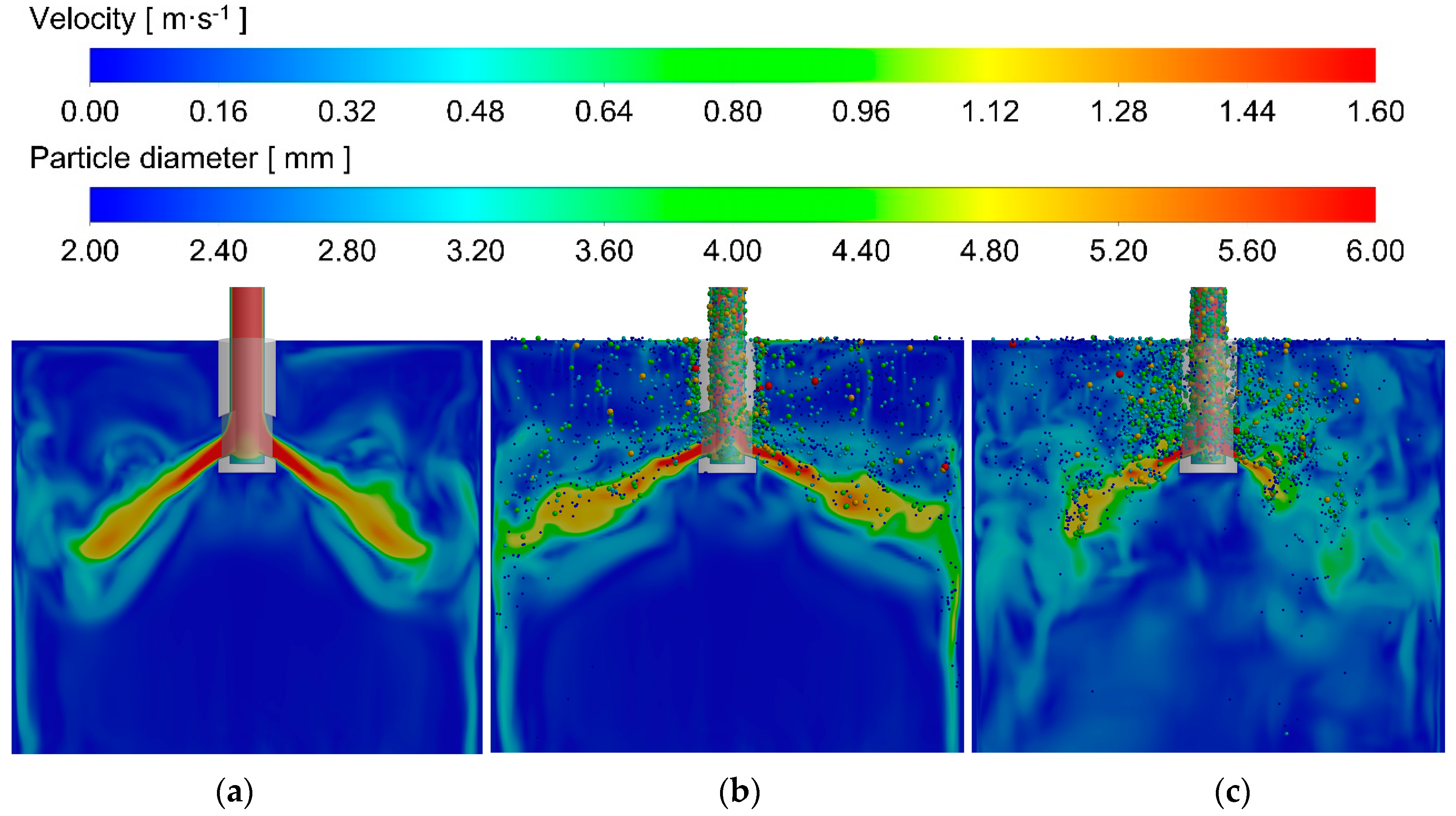
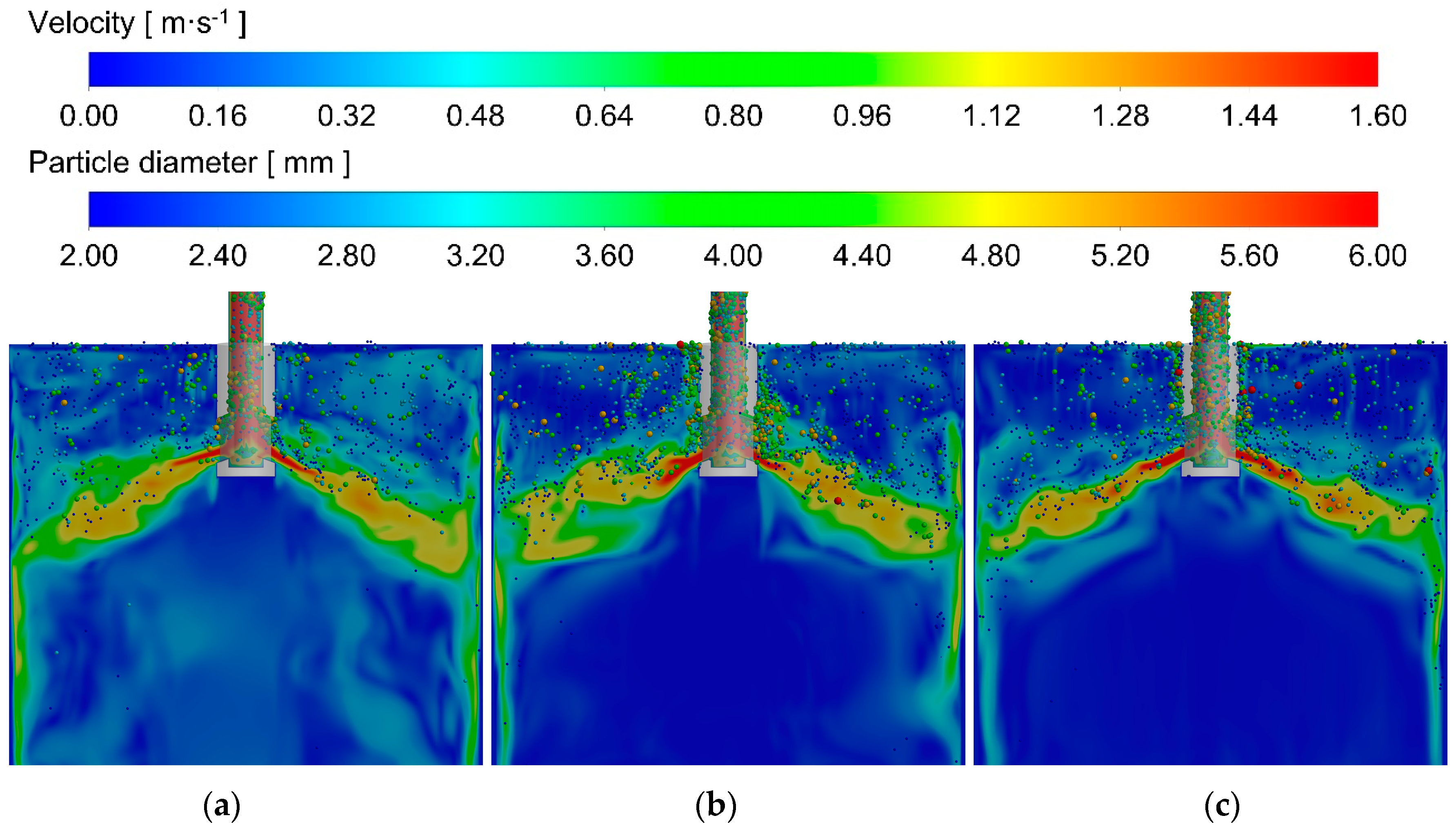
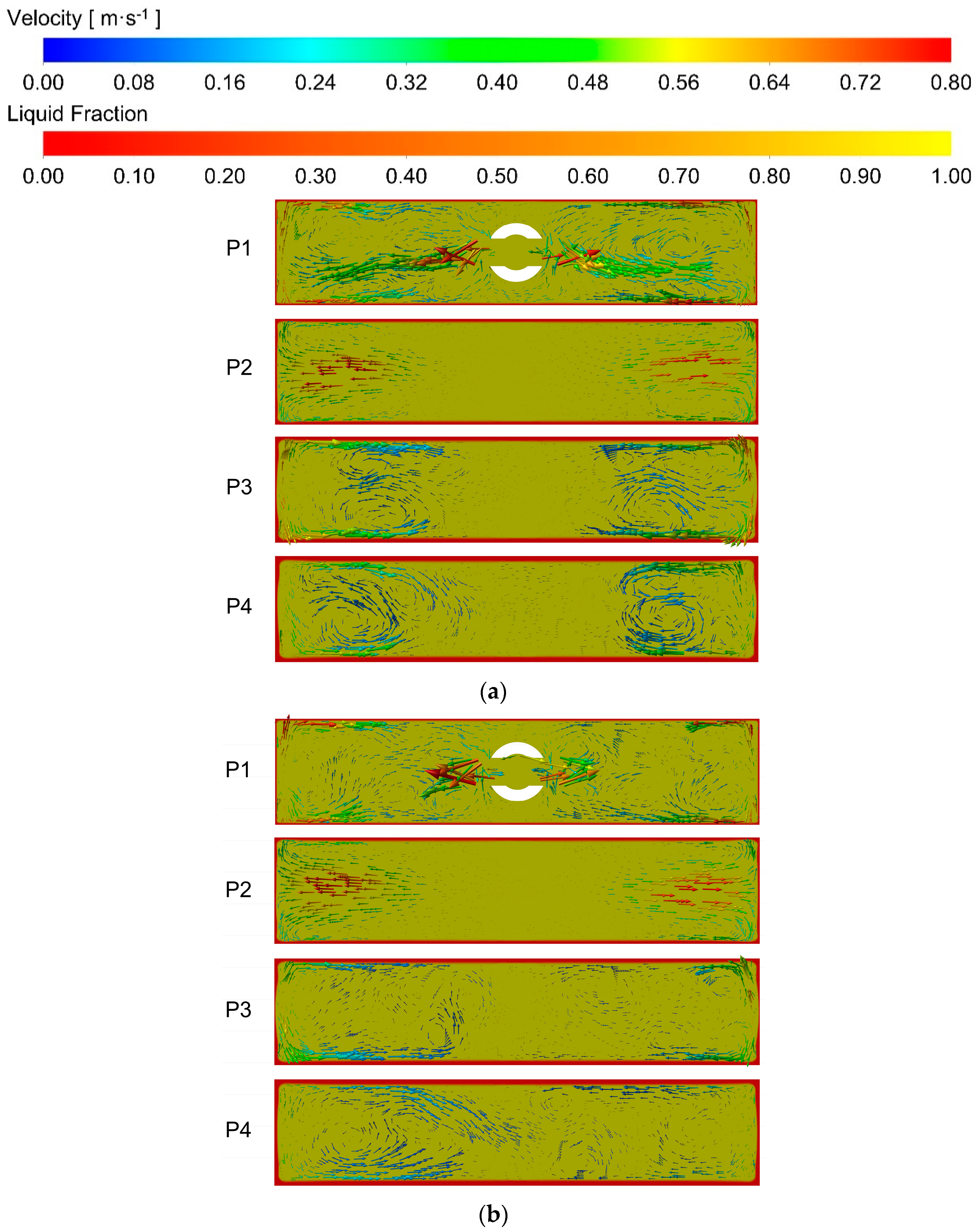
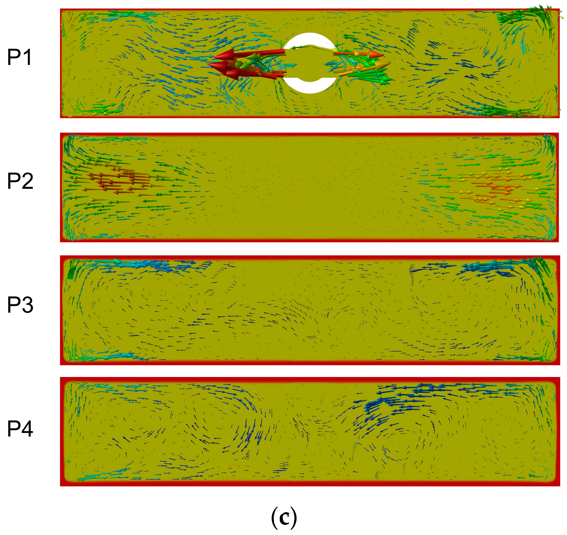
3.3. Effects of Argon Flow Rate and EMBr on Mold Flow Field

Figure 7 shows the time average velocity contour and vector diagram of the mold flow field under EMBr Mode 3 and at different argon flow rates. As shown in Figure 7a, when the argon flow rate is 0 L·min⁻¹, the area where the jet velocity near the port is greater than 1.44 m·s⁻¹ is larger, and the angle between the jet and the vertical direction is smaller. The jet from the port is subjected to the EMBr at the lower part of the mold, which reduces jet velocity. Under the action of the upper magnetic field, the upper circulating flow is further weakened, resulting in a low velocity on the mold surface. As shown in Figure 7b, when the argon flow rate is 6 L·min⁻¹, due to the upward floating effect of argon bubbles, the jet direction of liquid steel from the port rises, which strengthens the upward circulation flow of liquid steel. Therefore, the surface velocity of the mold increases. As shown in Figure 7c, when the argon flow rate is further increased to 10 L·min⁻¹, the number of argon bubbles near the SEN increases too much, resulting in the disorder of the jet. Under the action of EMBr, the kinetic energy of the jet decreases greatly, resulting in the weakening of the upper circulating flow, which is not conducive to the control of the flow pattern and may lead to violent fluctuation near the SEN. By comprehensively comparing the flow field in the mold under the above three argon flow rates, it is more appropriate that the argon flow rate be 6 L·min⁻¹.

Figure 8 is the time average velocity contour and vector diagram of the flow field in the mold under the different EMBr modes when the argon flow rate is 6 L·min⁻¹. Figure 8a shows that under the condition of EMBr Mode 1, after the liquid steel jet from the port impacts the narrow face of the mold, it is divided into upper and lower streams. The flow field mode is a typical double-roll flow. Due to the large impact of upstream and downstream velocities, it may lead to violent fluctuation and slag entrainment risk. As shown in Figure 8b, under the condition of EMBr Mode 2, the jet from the port is well restrained by the strong magnetic field excited by the lower coil current, and the jet speed decreases. Although the weak magnetic field in the upper part has a weak braking effect on the upper circulating flow at this time, it still makes the low-speed area larger compared with that in Figure 8a. As shown in Figure 8c, under the condition of EMBr Mode 3, the jet from the port is well restrained by the strong magnetic field excited by the lower coil current. While the jet velocity decreases, the current in the upper coil increases the upper magnetic field, and the upper circulating flow is significantly braked. Therefore, the surface velocity of the mold is greatly reduced, and the low-speed area in the upper part of the mold is further increased. At the same time, because argon bubbles float up near the SEN, it can be clearly seen that some liquid steel moves directly to the surface driven by argon bubbles.

3.4. Effects of Argon Flow and EMBr on Argon Bubble Distribution

Figure 9 shows the contour diagram of instantaneous velocity and distribution of argon bubbles in the mold under EMBr Mode 3 and at different argon flow rates. When argon gas is not injected, the jet velocity is large, and the angle between the jet and the SEN is small. When the argon flow rate is 6 L·min⁻¹, the steel liquid near the SEN is affected by the floating of argon bubbles. With the increase in argon flow rate to 10 L·min⁻¹, the influence of floating of argon bubbles is gradually significant, and the jet becomes disordered, and jet velocity decreases significantly due to the concentration of argon bubbles floating up near the SEN. The number of argon bubbles that can move near the narrow face of the mold is significantly reduced, and more argon bubbles float near the SEN, which will aggravate the fluctuation near the SEN and increase the risk of slag entrapment and slag layer breaking. At this time, the excessive argon flow rate leads to the instability of the flow field in the mold, and the risk of defect of argon bubbles increases on the surface of the automobile exposed panel.

Figure 10 demonstrates the contour diagram of instantaneous velocity and distribution of argon bubbles in the mold at argon flow rate of 6 L·min⁻¹ and under different EMBr modes. Under the condition of EMBr Mode 1, the upper and lower circulating flow velocities are very large. Some argon bubbles are washed into the deep site of the mold with the lower circulating flow, following the liquid steel to move near the solidified shell, which may be captured by the solidified shell, resulting in bubble defects. Under the condition of Mode 2, due to the inhibition of the lower magnetic field excited by the lower coil, the velocity of the lower circulation stream decreases significantly. It also inhibits the penetration of large-size argon bubbles into the mold, but it has little effect on the small-size argon bubbles, and many small-size argon bubbles can still move deep into the mold. Under the condition of Mode 3, the magnetic field has an obvious braking effect on the jet. The number of argon bubbles following the jet to the narrow face of the mold decreases, and the velocity near the meniscus decreases significantly, which reduces the risk of slag entrapment.

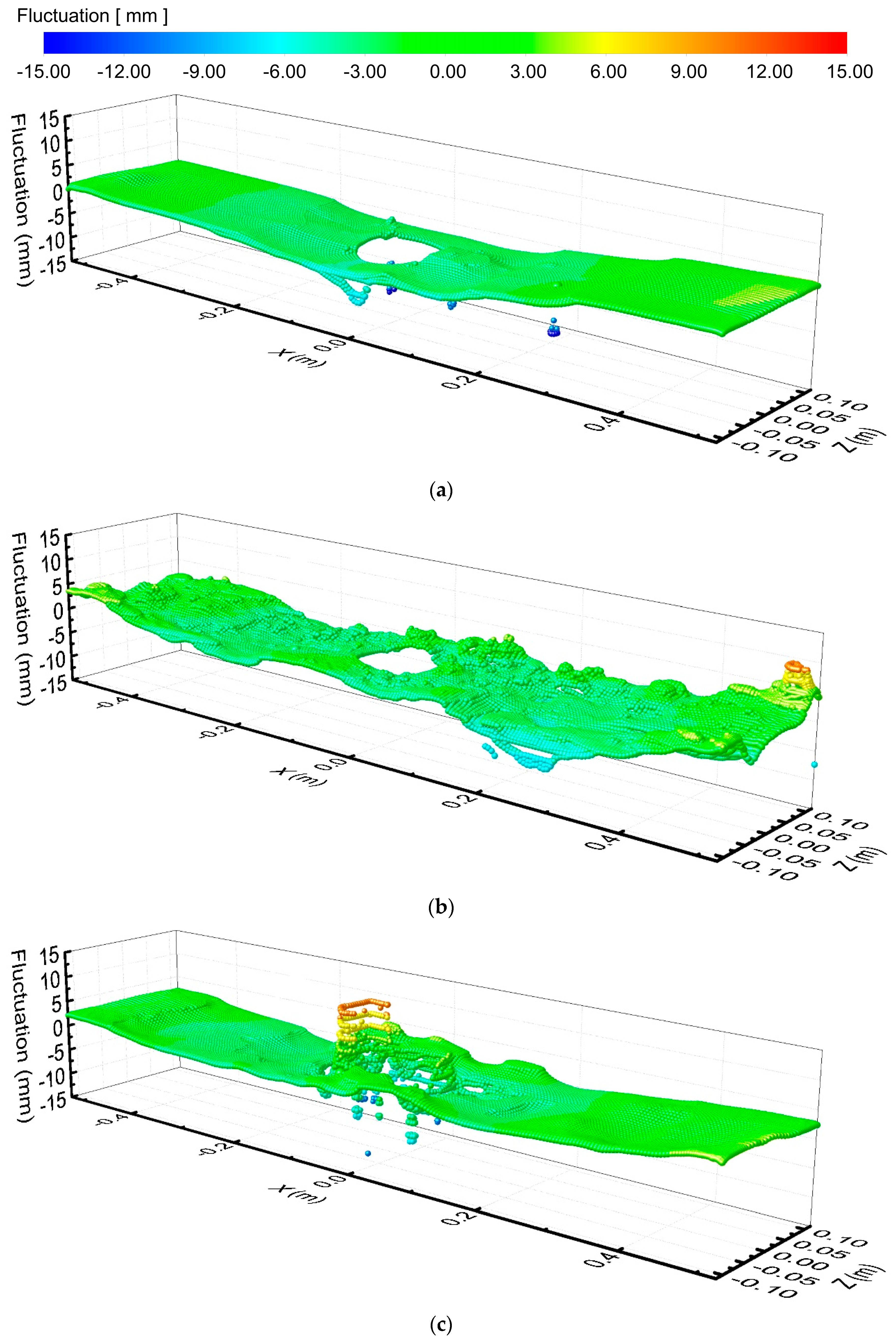
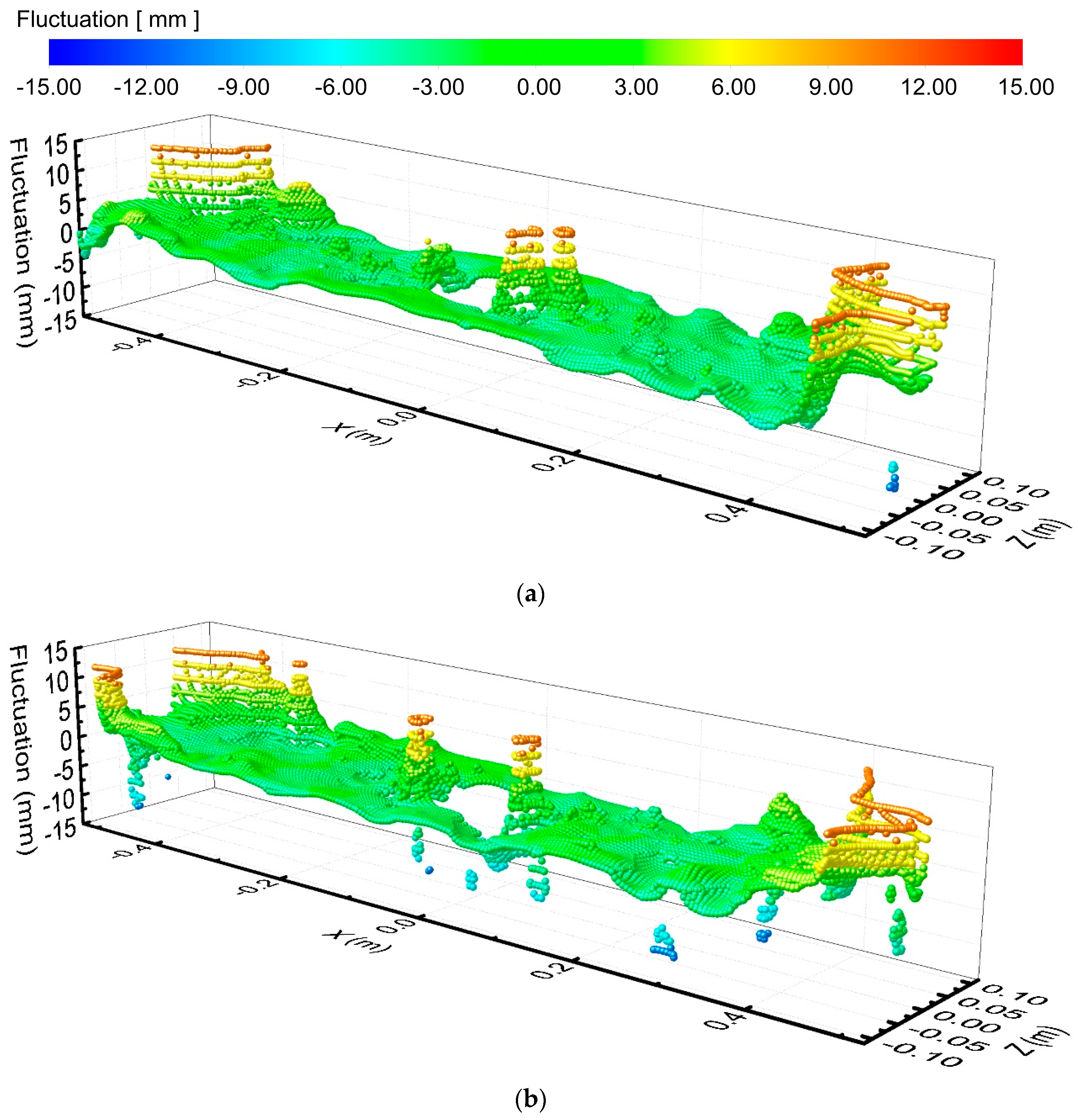
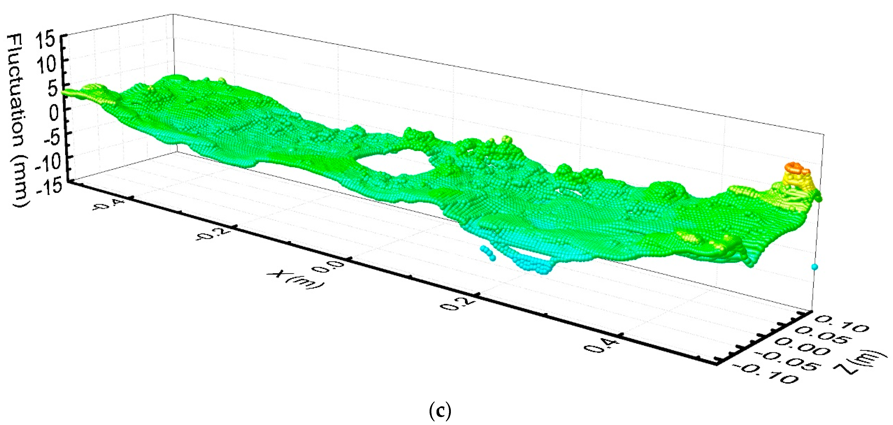
3.5. Fluctuation on Mold Surface

Figure 11 shows the fluctuation diagram of mold surface under EMBr Mode 3 with the strongest EMBr action and at different argon flow rates. When the argon flow rate is 0 L·min⁻¹, the upper circulating flow is weak due to the braking effect of the magnetic field, and the velocity of the mold surface is very low, so the fluctuation is very gentle. When the argon flow rate is 6 L·min⁻¹, due to the introduction of argon into the SEN, the floating of argon bubbles has an impact on the liquid fluctuation level of the mold and disturbs the liquid level, resulting in a slight increase in fluctuation, but the liquid fluctuation level is still within a reasonable range. However, when the argon flow rate is further increased to 10 L·min⁻¹, a large number of argon bubbles escape near the SEN wall, resulting in a sharp increase in the fluctuation of the liquid level, with local areas exceeding 10 mm, which will significantly increase the risk of slag entrapment and reduce the surface quality of the automobile exposed panel.

Figure 12 is the fluctuation diagram of the mold surface at argon flow of 6 L·min⁻¹ and under different EMBr modes. Under the condition of Mode 1 without EMBr, the fluctuation of 1050 mm width mold will be very violent under the condition of high casting speed of 1.9 m·min⁻¹, and the fluctuation near the narrow face of the mold and the SEN will even exceed 10 mm. Under the condition where only the lower coil is with the current in Mode 2, due to the weak upper magnetic field and limited ability to suppress the liquid level fluctuation, the fluctuation of the mold surface is still large, and the fluctuation near the narrow face of the mold and the SEN will also exceed 10 mm. Under the condition of Mode 3 where the upper and lower coils are with the current, the upper and lower magnetic fields jointly inhibit the upper circulating flow and movement of argon bubbles. The fluctuation range of most areas of the mold surface is no more than 5 mm, and the fluctuation of the mold surface is within a reasonable range, even at the high casting speed of 1.9 m·min⁻¹.

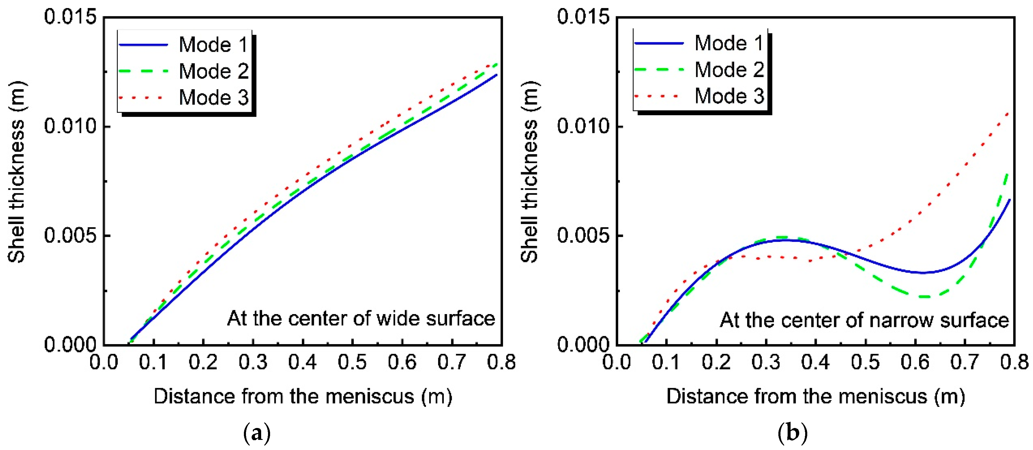
3.6. Effect of EMBr on Solidified Shell

Figure 13 shows the velocity vector diagram and liquid volume fraction contour diagram at argon gas flow rate of 6 L·min⁻¹ on different reference planes and under the different EMBr modes. Compared with the P1 plane, under the condition of Mode 1 without the restraint of magnetic field, the jet has a great impact on the narrow face of the mold. Under the condition of Mode 2 and Mode 3, the jet is affected by EMBr, and the impact on the narrow face is significantly restrained. Compared with P2, P3 and P4 planes, it can be observed that after the jet impinges on the narrow face, part of the liquid steel will reflux along the wide face in the SEN direction in the mold. The reflux is very strong under the condition of Mode 1. It can be seen that the jet impinges on the narrow face greatly, and the reflux intensity further decreases significantly under the conditions of Mode 2 and Mode 3, which is conducive to the formation and growth of the solidified shell on the wide face, narrow face and at the corner.

Figure 14 is the variation of solidified shell thickness under different EMBr modes showing the change in shell thickness with depth at the center of the wide and narrow face. As shown in Figure 14a, under the condition of EMBr Mode 3, the shell thickness at the center of the wide face is greater than that in Mode 2, and the thickness in Mode 2 is greater than that in Mode 1. It can be seen from Figure 14b that under the conditions of Mode 1 and Mode 2, there is no EMBr or insufficient braking capacity for the jet, and the jet scours the narrow face violently, so that the shell thickness decreases in the range above 0.45 m from the mold surface. In Mode 3, the impact of the jet on the narrow face is well restrained. In the range above 0.45 m from the mold surface, the shell thickness of the narrow face shell is significantly greater than those in Mode 1 and Mode 2.

4. Conclusions

Considering the influence of the solidified shell and the mold flux, the flow field, distribution of argon bubbles, liquid level fluctuation and solidified shell thickness in the mold were studied under different argon flow rates and EMBr conditions with numerical simulation and high-temperature quantitative velocity measurement. The main conclusions are as follows:

(1)

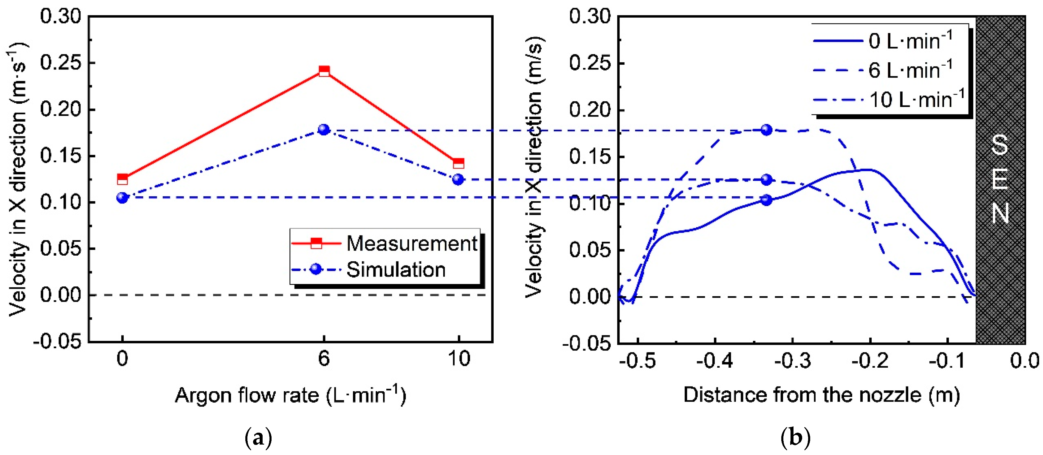
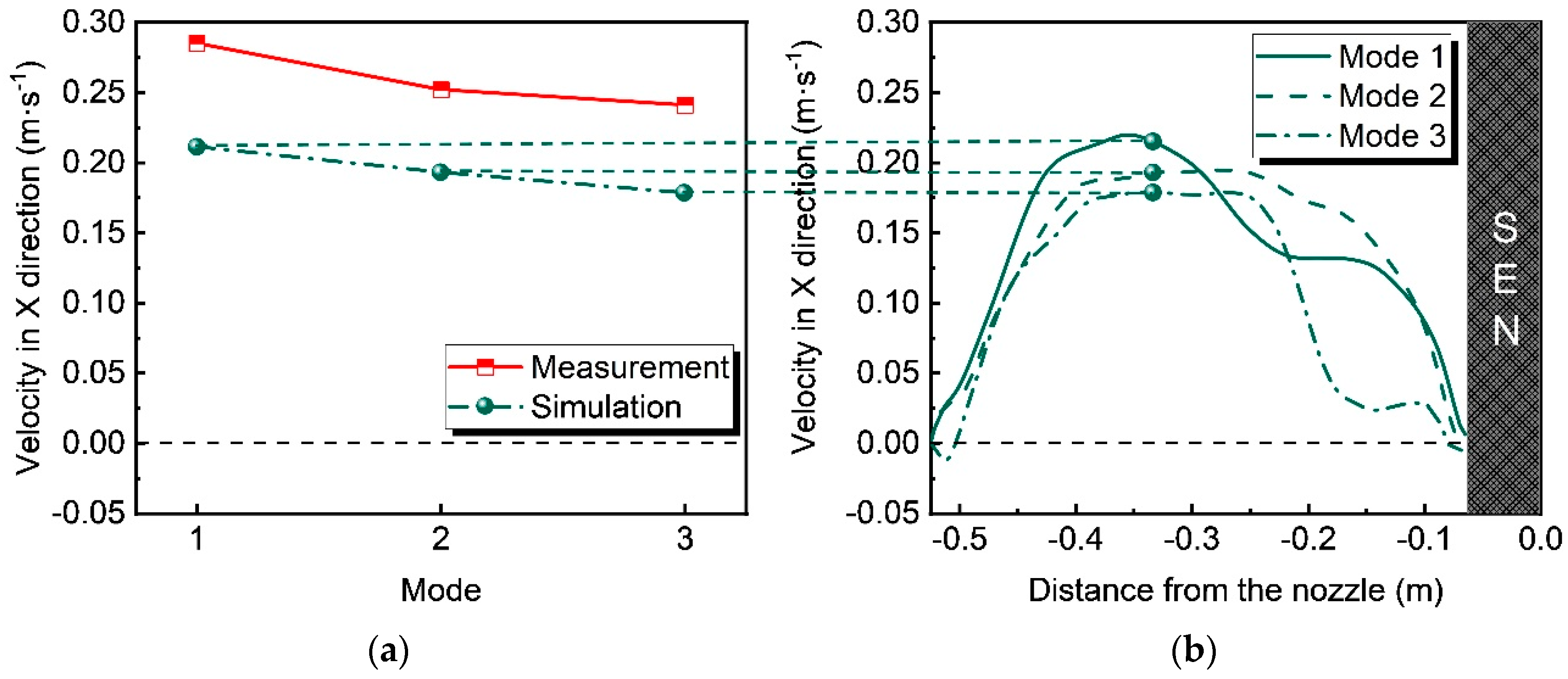
The calculated velocities on the mold surface are in good agreement with the measured values of the industrial experiment at high temperature with the rod deflection method. As the argon flow rate is increased from 0 to 6 L·min⁻¹ and 10 L·min⁻¹, both of the calculated and measured velocities on the mold surface first increase and then decrease. As the EMBr mode changes from Mode 1 without EMBr to Mode 2 with upper coil current 0 A and lower coil current 700 A, and then to Mode3 with upper coil current 300 A and lower coil current 700 A, both of the calculated and measured velocities on the mold surface gradually decrease.

(2)

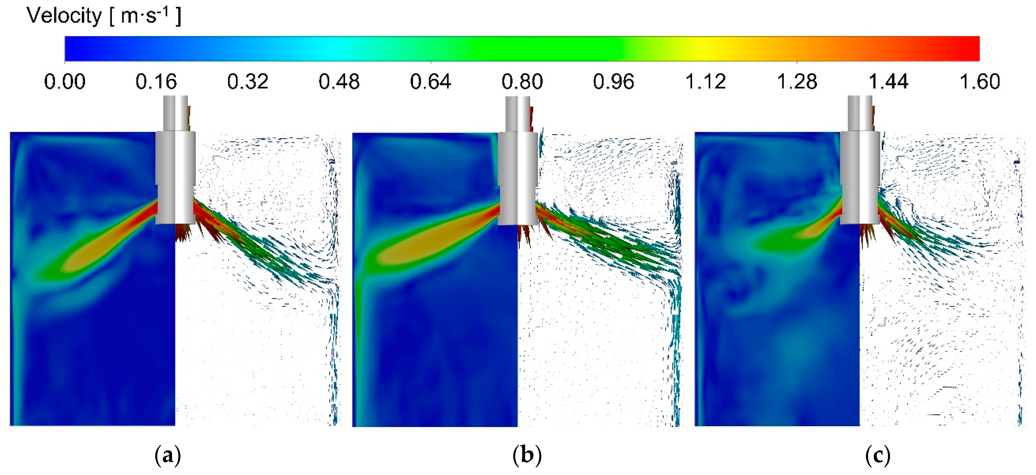
With EMBr Mode 3 and at the argon flow rate of 0 L·min⁻¹, the velocity on the mold surface is too low, which is not conducive to the melting of the mold flux. When the argon flow rate is 6 L·min⁻¹, the jet angle increases, and the velocity on the mold surface increases, which is conducive to heat and mass transfer near the meniscus. When the argon flow rate is further increased to 10 L·min⁻¹, the upper circulating flow is affected by floating up of more argon bubbles; the surface velocity of the mold decreases, and the liquid level fluctuation near the SEN increases.

(3)

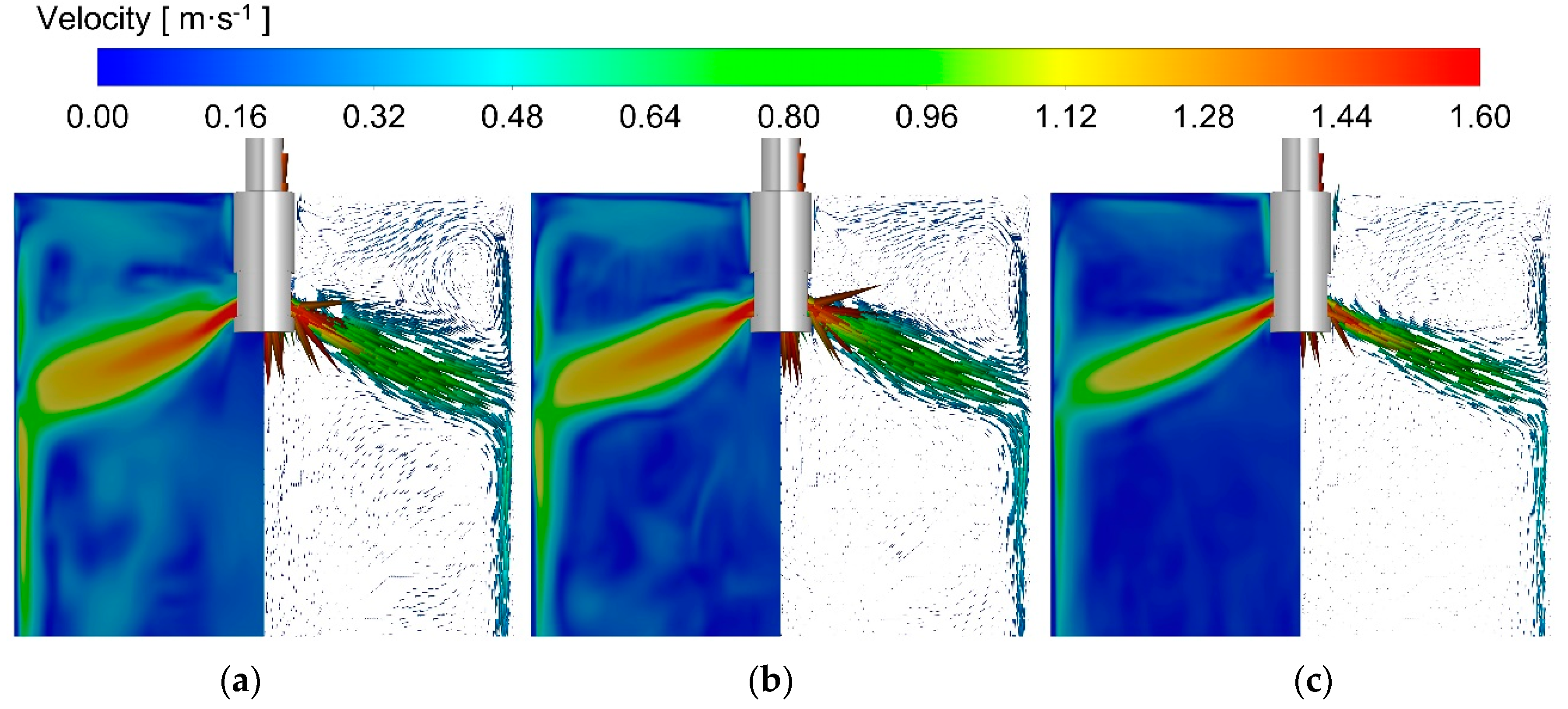
When the argon flow rate is 6 L·min⁻¹ and the casting speed is 1.9 m·min⁻¹, with EMBr Mode 1, the liquid level fluctuation is too large, which may lead to slag entrainment in the mold. With Mode 2, as the lower circulation stream is restrained by the lower magnitude field, the velocity on the mold surface decreases, but the liquid level fluctuation is still large. With Mode 3, both of the lower and upper circulation streams are restrained by the magnetic field, the velocity on the mold surface is reduced, and the fluctuation is at a relatively reasonable level.

(4)

With EMBr Mode 3, when the argon flow rate is 10 L·min⁻¹, due to the strong upward floating of argon bubbles, the jet at the port becomes disordered, and the liquid level fluctuation near the SEN wall intensifies, which increases the risk of slag entrainment and slag layer breaking, as well as the risk of argon bubbles being captured. When the argon flow rate is 6 L·min⁻¹, the liquid level fluctuation of the mold is in a reasonable range under the conditions of Mode 3. Therefore, it is reasonable to control the argon flow rate to be 6 L·min⁻¹.

(5)

With Mode 1 and Mode 2, due to no braking or insufficient braking capacity, the jet scours the narrow face violently, resulting in the decrease in thickness of the solidified shell in the range above 0.45 m from the mold surface. With Mode 3, as the impact of the jet on the narrow face is well restrained, the solidified shell thickness of the narrow surface is significantly greater than those in Modes 1 and 2 in the range above 0.45 m from the mold surface.

References

- Zhang, L.F.; Yang, S.B.; Cai, K.K.; Li, J.Y.; Wan, X.G.; Thomas, B.G. Investigation of fluid flow and steel cleanliness in the continuous casting strand. Metall. Mater. Trans. B 2007, 38, 63–83. [Google Scholar] [CrossRef]
- Yuan, Q.; Thomas, B.G.; Vanka, S.P. Study of transient flow and particle transport in continuous steel caster molds: Part I. Fluid flow. Metall. Mater. Trans. B 2004, 35, 685–702. [Google Scholar] [CrossRef] [Green Version]
- Yuan, Q.; Thomas, B.G.; Vanka, S.P. Study of transient flow and particle transport in continuous steel caster molds: Part II. Particle transport. Metall. Mater. Trans. B 2004, 35, 703–714. [Google Scholar] [CrossRef]
- Thomas, B.G.; Yuan, Q.; Mahmood, S.; Liu, R.; Chaudhary, R. Transport and Entrapment of Particles in Steel Continuous Casting. Metall. Mater. Trans. B 2014, 45, 22–35. [Google Scholar] [CrossRef]
- Jin, K.; Vanka, S.P.; Thomas, B.G. Large Eddy Simulations of Electromagnetic Braking Effects on Argon Bubble Transport and Capture in a Steel Continuous Casting Mold. Metall. Mater. Trans. B 2018, 49, 1360–1377. [Google Scholar] [CrossRef]
- Zhang, L.; Li, Y.; Wang, Q.; Yan, C. Prediction model for steel/slag interfacial instability in continuous casting process. Ironmak. Steelmak. 2015, 42, 705–713. [Google Scholar] [CrossRef]
- Hagemann, R.; Schwarze, R.; Heller, H.P.; Scheller, P.R. Model Investigations on the Stability of the Steel-Slag Interface in Continuous-Casting Process. Metall. Mater. Trans. B 2013, 44, 80–90. [Google Scholar] [CrossRef]
- Fei, P.; Min, Y.; Liu, C.J.; Jiang, M.F. Effect of continuous casting speed on mold surface flow and the related near-surface distribution of non-metallic inclusions. Int. J. Miner. Metall. Mater 2019, 26, 186–193. [Google Scholar] [CrossRef]
- Chen, W.; Ren, Y.; Zhang, L.; Scheller, P.R. Numerical Simulation of Steel and Argon Gas Two-Phase Flow in Continuous Casting Using LES plus VOF plus DPM Model. JOM 2019, 71, 1158–1168. [Google Scholar] [CrossRef]
- Takatani, K. Effects of electromagnetic brake and meniscus electromagnetic stirrer on transient molten steel flow at meniscus in a continuous casting mold. ISIJ Int. 2003, 43, 915–922. [Google Scholar] [CrossRef]
- Wang, Y.; Zhang, L. Fluid Flow-Related Transport Phenomena in Steel Slab Continuous Casting Strands under Electromagnetic Brake. Metall. Mater. Trans. B 2011, 42, 1319–1351. [Google Scholar] [CrossRef]
- Garcia-Hernandez, S.; Morales, R.D.; Torres-Alonso, E. Effects of EMBr position, mould curvature and slide gate on fluid flow of steel in slab mould. Ironmak. Steelmak. 2010, 37, 360–368. [Google Scholar] [CrossRef]
- Xu, L.; Wang, E.; Karcher, C.; Deng, A.; Xu, X. Numerical Simulation of the Effects of Horizontal and Vertical EMBr on Jet Flow and Mold Level Fluctuation in Continuous Casting. Metall. Mater. Trans. B 2018, 49, 2779–2793. [Google Scholar] [CrossRef]
- Singh, R.; Thomas, B.G.; Vanka, S.P. Large Eddy Simulations of Double-Ruler Electromagnetic Field Effect on Transient Flow During Continuous Casting. Metall. Mater. Trans. B 2014, 45, 1098–1115. [Google Scholar] [CrossRef] [Green Version]
- Cho, S.M.; Thomas, B.G.; Kim, S.H. Transient Two-Phase Flow in Slide-Gate Nozzle and Mold of Continuous Steel Slab Casting with and without Double-Ruler Electro-Magnetic Braking. Metall. Mater. Trans. B 2016, 47, 3080–3098. [Google Scholar] [CrossRef]
- Liu, Z.; Li, L.; Li, B. Large Eddy Simulation of Transient Flow and Inclusions Transport in Continuous Casting Mold under Different Electromagnetic Brakes. JOM 2016, 68, 2180–2190. [Google Scholar] [CrossRef]
- Sarkar, S.; Singh, V.; Ajmani, S.K.; Singh, R.K.; Chacko, E.Z. Effect of Argon Injection in Meniscus Flow and Turbulence Intensity Distribution in Continuous Slab Casting Mold Under the Influence of Double Ruler Magnetic Field. ISIJ Int. 2018, 58, 68–77. [Google Scholar] [CrossRef] [Green Version]
- Yin, Y.; Zhang, J.; Ma, H.; Zhou, Q. Large Eddy Simulation of Transient Flow, Particle Transport, and Entrapment in Slab Mold with Double-Ruler Electromagnetic Braking. Steel Res. Int. 2021, 92, 2000582. [Google Scholar] [CrossRef]
- Sarkar, S.; Singh, V.; Ajmani, S.K.; Ranjan, R.; Rajasekar, K. Effect of Double Ruler Magnetic Field in Controlling Meniscus Flow and Turbulence Intensity Distribution in Continuous Slab Casting Mold. ISIJ Int. 2016, 56, 2181–2190. [Google Scholar] [CrossRef] [Green Version]
- Yu, H.; Zhu, M. Numerical simulation of the effects of electromagnetic brake and argon gas injection on the three-dimensional multiphase flow and heat transfer in slab continuous casting mold. ISIJ Int. 2008, 48, 584–591. [Google Scholar] [CrossRef] [Green Version]
- Li, Z.; Zhang, L.; Ma, D.; Wang, E. Numerical Simulation on Flow Characteristic of Molten Steel in the Mold with Freestanding Adjustable Combination Electromagnetic Brake. Metall. Mater. Trans. B 2020, 51, 2609–2627. [Google Scholar] [CrossRef]
- Jin, K.; Vanka, S.P.; Thomas, B.G. Large Eddy Simulations of the Effects of EMBr and SEN Submergence Depth on Turbulent Flow in the Mold Region of a Steel Caster. Metall. Mater. Trans. B 2017, 48, 162–178. [Google Scholar] [CrossRef]
- Yin, Y.; Zhang, J. Mathematical Modeling on Transient Multiphase Flow and Slag Entrainment in Continuously Casting Mold with Double-ruler EMBr through LES plus VOF plus DPM Method. ISIJ Int. 2021, 61, 853–864. [Google Scholar] [CrossRef]
- Zhang, T.; Yang, J.; Jiang, P. Measurement of Molten Steel Velocity near the Surface and Modeling for Transient Fluid Flow in the Continuous Casting Mold. Metals 2019, 9, 36. [Google Scholar] [CrossRef] [Green Version]
- Zhang, T.; Yang, J.; Xu, G.J.; Liu, H.J.; Zhou, J.J.; Qin, W. Effects of operating parameters on the flow field in slab continuous casting molds with narrow widths. Int. J. Miner. Metall. Mater 2021, 28, 238–248. [Google Scholar] [CrossRef]
- Ma, C.; He, W.Y.; Qiao, H.S.; Zhao, C.L.; Liu, Y.B.; Yang, J. Flow Field in Slab Continuous Casting Mold with Large Width Optimized with High Temperature Quantitative Measurement and Numerical Calculation. Metals 2021, 11, 261. [Google Scholar] [CrossRef]
- Jiang, P.; Yang, J.; Zhang, T.; Xu, G.; Liu, H.; Zhou, J.; Qin, W. Optimization of Flow Field in Slab Continuous Casting Mold with Medium Width Using High Temperature Measurement and Numerical Simulation for Automobile Exposed Panel Production. Metals 2020, 10, 9. [Google Scholar] [CrossRef] [Green Version]
- Liu, Y.; Yang, J.; Huang, F.; Zhu, K.; Liu, F.; Gong, J. Comparison of the Flow Field in a Slab Continuous Casting Mold between the Thicknesses of 180 mm and 250 mm by High Temperature Quantitative Measurement and Numerical Simulation. Metals 2021, 11, 1886. [Google Scholar] [CrossRef]
- Chaudhary, R.; Thomas, B.G.; Vanka, S.P. Effect of Electromagnetic Ruler Braking (EMBr) on Transient Turbulent Flow in Continuous Slab Casting using Large Eddy Simulations. Metall. Mater. Trans. B 2012, 43, 532–553. [Google Scholar] [CrossRef]
- Liu, Y.B.; Yang, J.; Lin, Z.Q. Mathematical Modeling of Mold Flow Field and Mold Flux Entrainment Assisted With High-Temperature Quantitative Velocity Measurement and Water Modeling. Metall. Mater. Trans. B 2022, 53B. [Google Scholar] [CrossRef]
- Shur, M.L.; Spalart, P.R.; Strelets, M.K.; Travin, A.K. A hybrid RANS-LES approach with delayed-DES and wall-modelled LES capabilities. Int. J. Heat Fluid Flow 2008, 29, 1638–1649. [Google Scholar] [CrossRef]
- Liu, Y.B.; Yang, J.; Ma, C.; Zhang, T.; Gao, F.B.; Li, T.Q.; Chen, J.L. Mathematical modeling of flow field in slab continuous casting mold considering mold powder and solidified shell with high temperature quantitative measurement. J. Iron Steel Res. Int. 2022, 29, 445–461. [Google Scholar] [CrossRef]