Article

Hybrid Method for Endpoint Prediction in a Basic Oxygen Furnace

1
Department of Materials Science and Engineering, University of Toronto, 184 College Street, Toronto, ON M5S 3E4, Canada
2
R&D Division, Tata Steel Ltd., NML Inside Rd., Burma Mines Market, Burma Mines, Susnigerya, Jamshedpur 831001, India
*
Author to whom correspondence should be addressed.
Metals 2022, 12(5), 801; https://doi.org/10.3390/met12050801
Submission received: 22 February 2022 / Revised: 31 March 2022 / Accepted: 3 May 2022 / Published: 5 May 2022
(This article belongs to the Special Issue Oxygen Steelmaking Process)

Abstract

:
Strict monitoring and prediction of endpoints in a Basic Oxygen Furnace (BOF) are essential for end-product quality and overall process efficiency. Existing control models are mostly developed based on thermodynamic principles or by deploying advanced sensors. This article aims to propose a novel hybrid algorithm for endpoint temperature, carbon, and phosphorus, based on heat and mass balance and a data-driven technique. Three types of static models were established in this study: firstly, theoretical models, based on user-specified inputs, were formulated based on mass and energy balance; secondly, artificial neural networks (ANN) were developed for endpoints predictions; finally, the proposed hybrid model was established, based upon exchanging outputs among theoretical models and ANNs. Data of steelmaking production details collected from 28,000 heats from Tata Steel India were used for this article. Machine learning model validation was carried out with five-fold cross-validation to ensure generalizations in model predictions. ANNs are found to achieve better predictive accuracies than theoretical models in all three endpoints. However, they cannot be directly applied in any steelmaking plants, due to possible variations in the production setting. After applying the hybrid algorithm, normalized root mean squared errors are reduced for endpoint carbon and phosphorus by 3.7% and 9.77%.

1. Introduction

The Basic Oxygen Furnace (BOF) is a key process in the global steelmaking industry due to its high productivity and cost-efficiency, and it is implemented in around 65% of global steelmaking plants [1,2]. Over the past decade, the steelmaking industry has faced continuous economic and environmental challenges, including a 100% increase in the price of iron ore [3]. As a result, to fulfil the steel product pricing requirement and ensure an uninterrupted supply of raw material, the source of iron ore may change abruptly. Such sudden change in iron ore sources may change the quality of iron ore, and, eventually, can change the quality of hot metal produced from the blast furnace. For instance, the phosphorus (P) content of hot metal can occasionally change, due to the high P content in iron ore. This change in iron ore quality can affect the processing of hot metal in a basic oxygen furnace, in terms of alteration in blowing periods, flow of input oxygen, etc. The problem of over-blow or under-blow can also be observed, which creates problems for downstream operators. The same issues can arise if there is rapid fluctuation in hot metal carbon and silicone content. Close control of such situations is not possible by human interventions only, and fast automated support is needed. An assistance model can be extremely useful for operators to predict the operating conditions upon observing any such fluctuation in hot metal quality. Thus, in the production process, accurate predictions on endpoint steel chemistries and temperature (T) can ensure final product quality, as well as process efficiency.
BOF is a complex multi-variate and multi-phase process, subject to oscillations in input materials and extreme environments. During the process, pure oxygen is injected into the furnace at a supersonic speed onto the surface of hot metal (HM) in order to elevate the furnace temperature and remove impurities through oxidation reactions. Endpoint compositions and endpoint temperature refer to the elemental content and temperature of the molten steel when the oxygen blowing process is completed. Endpoint carbon (C) directly determines the strength and brittleness of steel; increased P content in steel can lead to subpar ductility, toughness, and embrittlement; endpoint T plays a crucial factor in determining efficiency for subsequent processes, such as secondary refining and continuous casting [1,4]. The existing process control models for BOF can be roughly categorized into three groups: (i) online measurement models, (ii) theoretical models, and (iii) data-driven models [5].
Online measurement models involve the deployment of advanced sensors and equipment, such as sub-lance systems and off-gas analyzers [6,7,8]. These models can predict the endpoints for each heat during processing by means of continuous sensing. Thus, these models require large capital and maintenance costs, which directly increase the cost of steel. For example, Li et al. dynamically predicted off-gas formation by deriving a reaction kinetics-based mathematical model in a top-blown converter [9]. Cunha et. al. developed a dynamic model which could forecast endpoints and correct the process parameters using machine learning (ML)-based prediction and inverse models [10].
Mechanism models for predicting endpoint chemistries and temperature can be categorized into static models and dynamic models. Mechanism static models are usually established based on heat and mass balance during the process, and they mostly depend on static operation parameters and the stability of raw material characteristics. Heat balance model calculation includes the balance of input and output energy for a system at equilibrium. Input heat consists of the sensible heat of each input material, such as hot metal and scrap (for preheated scrap only) and dissolution heat of impurities, i.e., C, Si, Mn, and P in liquid iron. On the other hand, heat output is comprised of sensible heats of steel, sensible heats of slag, sensible heats of waste gases and heat of scrap melting. In order to calculate the sensible heats of these components, mass balance needs to be performed to determine their respective weights. Thus, heat and mass balance-based models can successfully identify the end chemical composition and temperature of liquid steel after heat making. A pioneer study on heat and mass balance in a BOF process was performed by Philbrook [11]. He presented the method of performing these calculations comprehensively. Slatosky developed a heat and mass balance-based static model to predict the end point temperature of BOF [12]. He also validated his calculations using data obtained from mill trials. Meyer et al. identified that error in FeO prediction by incorrect estimation of oxygen consumption in the formation of FeO and CO2 can lead to substantial deviation in endpoint temperature prediction [13]. In 1981, Neto established a solution-based heat and mass balance theoretical model to forecast endpoint carbon and temperature, but subpar prediction accuracy was found in the model, due to the theoretical assumptions in parameters [14]. Fruehan et al. developed a heat balance model to calculate minimum theoretical energy and validated that against real plant data [15]. Madhavan et al. applied a mass and energy balance model in oxygen steelmaking and validated their model against plant data [16,17]. Such models may suffer from the unrealistic assumption of equilibrium, as well as the highly volatile raw material components. Over the past several decades, a tremendous amount of research has been conducted on phosphorus removal, specifically in steelmaking, based on thermodynamic principles [18,19,20]. In the 1940s, Balajiva and Vijragupta reported that increasing the concentrations of CaO and FeO result in favor of phosphorus partition [18]. Suito and Inuoi concluded that dephosphorization accelerates with an increasing concentration of CaO in the slag [19]. Prediction of endpoint phosphorus is important because it is a determining factor for processing time. Optimized phosphorus content can help in reducing specific consumptions and improve the life of refractory lining. The equation for calculating the phosphorus partition ratio, established by Suito and Inuoi, is given by,
log % P % P = 0.072 % CaO + 0.3 % MgO + 0.6 % P 2 O 5 + 0.2 % MnO + 1.2 % CaF 2 0.5 % Al 2 O 3 + 2.5 log % Fe total + 11570 T 10.52
where (A) and (B) represent a species in the hot metal phase and slag phase respectively, T is the turndown temperature, and (%A) corresponds to the weight percentage of any component A. Phosphorus partition is chronologically improved through a lot of research using a combination of experimental and statistical analysis [21,22,23,24,25,26,27]. One of the limitations of the mechanism static model is the incapability of predicting both chemical compositions and temperature with time during the blowing process. To overcome such a limitation, researchers have developed mechanism static models by incorporating additional process variables [28,29]. In 2015, Sarkar et al. proposed a mathematical model for predicting the composition evolutions of slag-metal compositions by modeling the emulsion phenomena in three separate reactors with the incorporation of continuous process parameters, such as lance height. This model was able to predict many features of BOF process qualitatively well [28]. Recently, Biswas et al. further advanced this framework by including chemical reactions involving phosphorus and manganese. This model also incorporated a new mechanism reaction before the formation of emulsion, and it was capable of simulating the reversion of manganese and phosphorus in the middle of BOF blowing [29]. In the present manuscript, only the mechanism static model based on heat and mass balance is considered for formulation.
Data-driven static models are prominent in recent trends because they can significantly improve correlation among input and output features. With increasing computational power and availability of data, many researchers have successfully established endpoint prediction models by using statistical and machine learning techniques [5,30,31,32,33,34,35,36,37,38,39]. In 2010, Wang et al. proposed using mutual information as the input variable selection technique paired with an input weighted support vector machine to predict endpoint carbon of the BOF process. The model was capable of effectively selecting useful process parameters and improving forecasting accuracy [2]. Han et al. proposed an algorithm that combines particle swarm optimization, independent component analysis, and radial basis function neural network to predict endpoint carbon and temperature of BOF steelmaking [36]. In 2011, Cai et al. applied density-based spatial clustering of applications with a noise clustering algorithm and a radial-basis function neural network to predict endpoint temperature [39]. In 2019, Chattopadhyay and Kumar proposed building prediction models by using multiple linear regression (MLR) for two plants, where they presented necessary verification measures to incorporate the MLR algorithm [30]. More recently, Phull et al. established a gaussian mixture model (GMM) paired with decision tree-based twin support vector machine (TWSVM) based on slag chemistry and tapping temperature, to predict endpoint phosphorus [31]. A greater degree of P-partition can be achieved by using their proposed method. These results of data-driven models have shown effective improvements in prediction accuracy over conventional theoretical models.
In general, theoretical models that use thermodynamic principles are beneficial to understanding the reactions taking place in BOF steelmaking. However, these models tend to be established based on homogeneity of physiochemical reactions and slag compositions at equilibrium, which is unlikely to be achieved in BOF production, due to the nature of the multi-phase and multi-variate process. On the other hand, machine learning is a fast-growing area of research, due to its superb computational power in nonlinearity modeling, which can compensate for the deficiencies of traditional theoretical models. However, ML can be difficult to interpret and is sometimes referred to as a “black-box”, because it can contain thousands of parameters and the model can be hard to comprehend. In addition, endpoint prediction models that are developed based on ML techniques tend to be plant-specific, and they cannot be applied in any other steelmaking plants due to potential variations in production settings. Before the emergence of machine learning, the majority of the BOF process models were developed based on thermodynamic principles.
In this paper, a novel hybrid model to predict endpoint T, C, and P was established by using theoretical framework coupled with data-driven techniques. To begin with, a slag chemistry model was established by using static parameters to predict slag composition, which was incorporated to develop the theoretical model. Theoretical models for endpoint temperature, carbon, and phosphorus were developed based on heat and mass balance with static parameters and the slag chemistry model. Then, three machine learning models using ANN were developed for endpoint temperature, carbon, and phosphorus. In the end, the hybrid algorithm was carried out by creating a workflow that allows exchange of input and output among theoretical models and data-driven models. In contrast to theoretical models, the hybrid algorithm can reduce the number of assumptions and simplifications involved and ultimately improve predictive accuracies. In addition, the involvement of theoretical models within the hybrid architecture can effectively improve comprehensive understanding in the metallurgical process, and the presence of theoretical models allows the hybrid model to be applied in any steelmaking plant, disregarding variations in process parameters.

2. Theory and Methodology

As mentioned earlier, theoretical models and machine learning models have their own advantages regarding one another. All of the models in this paper are developed based on static parameters that are readily available before the beginning of the BOF process, which include hot metal chemistries, process parameters, and flux additions. On the other hand, lag parameters, such as slag chemistries, features that can only be measured when the BOF process is completed, are not directly used as input variables for model development. In this paper, a total of three different techniques were utilized for endpoint prediction model development. Firstly, theoretical models were established by formulating heat and mass balance of the BOF; secondly, an artificial neural network (ANN) was utilized to create three models for endpoint predictions; lastly, the proposed hybrid model algorithm was implemented, based on theoretical models and ANN by using Python 3.7. The theoretical and data-driven models’ developments are encapsulated using a flowchart as shown in Figure 1.

2.1. Nature of the Data

The proposed hybrid model algorithm was developed and tested on datasets obtained from Tata Steel India. The dataset consists of static features from 28,000 heats, including hot metal chemistries, process parameters, and flux additions. A detailed summary of features and endpoint values is presented in Table 1. Units for hot metal compositions and endpoint chemistries are provided in weight percentage (wt%), units for endpoint temperature and hot metal temperatures are in degrees Celsius; units for flux additions and hot metal weight are given in tons; the unit for oxygen volume is given in Nm3; and units for all other process parameters are in minutes.

2.2. Formulation of Mass and Energy Balance

The mass and energy balance model is crucial for modeling the BOF process, and it is commonly used as an in-house static model for controlling process parameters such as coolant addition or re-blowing. In this article, the heat and mass balance model was formulated to create theoretical models for predicting endpoint temperature, carbon, and phosphorus based on input static parameters.

2.2.1. Mass Balance

To create a static mass balance model, all materials entering and leaving the BOF system must be considered, and they can be expressed by a series of equations derived from elemental balance. In general, elemental balances can be categorized into four groups: metallic elemental balance, oxygen balance, carbon balance, and flux balance. Mass balance for metallic element X (can be Fe, Si, Mn, P) can be given by:
M a s s   o f   e l e m e n t   X i n   h o t   m e t a l + X   i n   I r o n   O r e + X   i n   S c r a p = M a s s   o f   e l e m e n t   X   i n   s t e e l + X i n   s l a g
oxygen balance can be described by:
M a s s   o f   o x y g e n   i n j e c t e d + o x y g e n   i n   i r o n   o r e + o x y g e n   i n   d o l o m i t e + o x y g e n   i n   l i m e = M a s s   o f   o x y g e n   i n   s l a g + o x y g e n   i n   O f f   G a s
carbon balance can be represented by:
M a s s   o f   c a r b o n   i n   h o t   m e t a l + c a r b o n     i n   S c r a p = M a s s   o f   c a r b o n   i n   s t e e l + c a r b o n   i n   o f f   g a s
and flux balance can be written in the following form:
M a s s   o f   f l u x   a d d i t i o n = M a s s   o f   C a O   a n d   M g O   i n   s l a g
Terms on the left side of the equal sign represent materials that enter the system, and terms on the right correspond to those that leave. By looking at Equations (2)–(5), steel and slag are two major components in the system outputs. Thus, to create a forecasting model for predicting steel chemistries, it is also necessary to predict slag chemistries to complete the overall mass balance calculation.

2.2.2. Slag Chemistry Model

Since slag parameters cannot be directly used as inputs to formulate mass balance, it is necessary to design a model specifically for slag chemistries. In order to create a slag chemistry model based on user-specified inputs, four simplifications and assumptions were considered for the formulation:
  • Silicon from hot metal is completely oxidized.
  • Weight percentage of CaO in slag is assumed to be the mean from the dataset, which is 51%.
  • Coolant added is in the form of pure Fe2O3.
  • Injected oxygen is completely consumed.
  • All the lime added to the process goes into the slag.
The slag chemistry model starts with creating a MLR model to predict theoretical slag basicity based on part of the user-specified parameters presented in Table 2. Theoretical slag basicity is an important parameter for refining and is given by Equation (6):
T h e o r e t i c a l   S l a g   B a s i c i t y = w e i g h t   p e r c e n t a g e   o f   C a O w e i g h t   p e r c e n t a g e   o f   S i O 2  
Based on the assumption that all of the silicon input is completely oxidized, the weight of SiO2 in slag can be calculated based on mass balance of silicon. Then, this value is multiplied by the predicted slag basicity from the regression model to provide the mass of CaO in slag, and slag weight can be computed based on the second assumption. Once the slag weight is determined, the weight percentages of MnO, MgO, Al2O3, and P2O5 can be calculated, based on elemental mass balance Equations (2)–(5). Lastly, the weight percentage of FeO can be determined by subtracting the weight percentages of all other components from 100%. The overall slag chemistry model calculations are represented using a flowchart as shown in Figure 2.

2.2.3. Endpoint Carbon Theoretical Model

Decarburization is the most extensive reaction during the BOF process. The majority of the carbon from liquid iron and scrap is oxidized into off-gas in the form of CO and CO2, and only a small amount of carbon is left in liquid steel, which is endpoint carbon. Instead of directly calculating endpoint carbon by formulating a carbon balance, the theoretical model developed in this paper uses oxygen balance to indirectly infer the amount of carbon present in liquid steel. The endpoint carbon theoretical model is closely dependent on one of the assumptions made earlier, which is that the oxygen injected is completely consumed. With the user-specified inputs and outputs from the slag chemistry model, the endpoint carbon model starts by calculating the mass of oxygen injected into the system through lance. Oxygen sourced from limestone, dolomite, and iron ore is also computed, and total weight of oxygen input can be calculated by using Equation (3). On the other hand, oxygen present in slag can be determined based on the predicted slag chemistries from the prior model. The difference between oxygen input and output refers to the amount of oxygen consumed for decarburization. From the dataset, the ratio between CO and CO2 in the off-gas is found to be relatively consistent; thus, a fixed ratio of 0.15 is applied based on iterative calculations. The overall flowchart of the endpoint carbon theoretical model is represented in Figure 3.

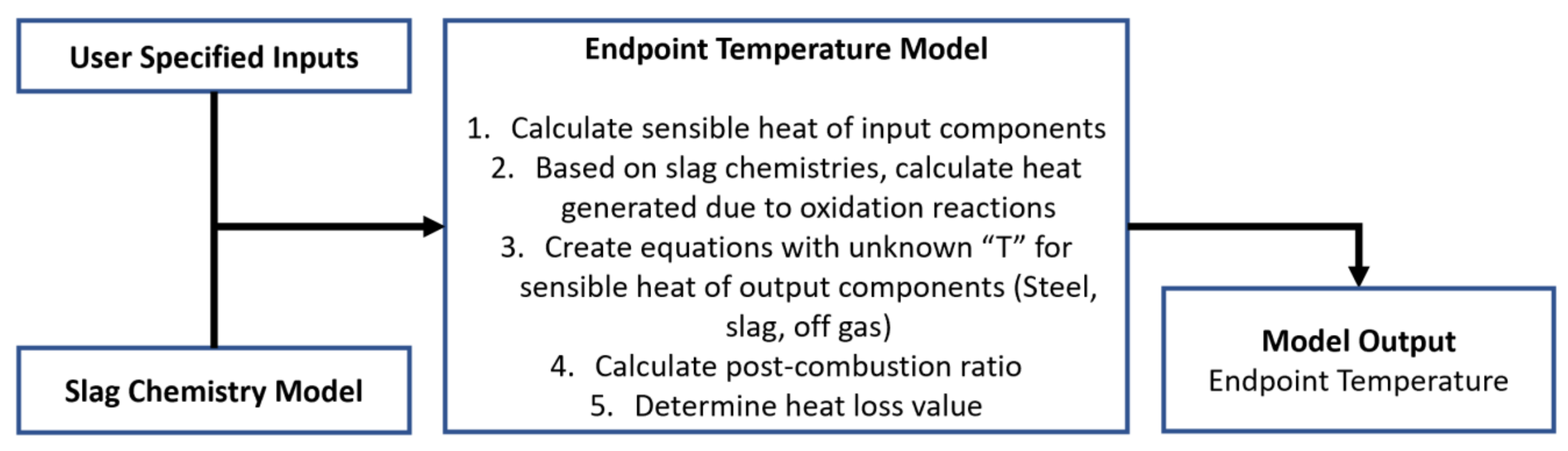
2.2.4. Heat Balance and Endpoint Temperature Theoretical Model

The assessment of heat balance is captured by establishing calculations that include the balance of input and output energy for a system at equilibrium. Heat input and output components in the BOF process can exist in various forms, such that input heat consists of sensible heat of each input material, such as hot metal and scrap (for preheated scrap only), and dissolution heat of impurities i.e., C, Si, Mn, and P in liquid iron. On the other hand, heat output is comprised of sensible heats of steel, sensible heats of slag, sensible heats of waste gases and heat of scrap melting. The heat balance for a BOF process can be formulated as follows:
Overall energy balance:
H e a t   i n p u t = H e a t   o u t p u t + H e a t   L o s s e s
Heat Input Components:
Heat input = Sensible heat of liquid iron + Heat of oxidation reactions
Heat Output Components:
H e a t   O u t p u t = S e n s i b l e   h e a t   o f   m o l t e n   s t e e l + s l a g + w a s t e   g a s + H e a t   o f   S c r a p   a n d   O r e   m e l t i n g  
Since no endpoint information is available for the formulation of heat balance in this study, four additional simplifications and assumptions are considered:
  • Sulfur is not considered for heat balance.
  • Weight percentages of iron and carbon in molten steel are assumed to be their respective medians from the dataset.
  • Flux and scrap additions are assumed to be charged at room temperature (25 °C).
  • Slag temperature is assumed to be 100 degrees Celsius higher than steel temperature [6].
  • Off-gas temperature is assumed to be 1600 °C [6].
In addition to the considered assumptions, the optimal heat loss and post-combustion ratio (PCR) in the heat balance model are investigated based on iterative calculations. According to the literature, heat loss for the oxygen steelmaking process ranges from 1.3% to 5.9% of the total heat input, and the PCR ratio ranges from 0.10 to 0.22 [6,7,16,40]. These value ranges are tried and tested to formulate the heat balance, and the values for heat loss and PCR are determined to be 5% and 0.15. The overall flowchart of the endpoint carbon theoretical model is represented in Figure 4.
Based on user-specified parameters, the sensible heat of liquid iron can be calculated with the weights of each component and their corresponding heat capacities:
S e n s i b l e   h e a t   o f   h o t   m e t a l = W H M F e % H M 298 T H M C p F e d T + C % H M 298 T H M C p C d T + H d i s s C + S i % H M 298 T H M C p S i d T + H d i s s S i + P % H M 298 T H M C p P d T + H d i s s P + M n % H M 298 T H M C p C d T + H d i s s M n
where WHM is the weight of hot metal, X%HM means weight percentage of X in hot metal, THM is the hot metal temperature, CpX represents specific heat of X, and HdissX corresponds to heat of dissolution of X. During the BOF process, impurities in the liquid iron are oxidized to form slags. With the results generated by the slag chemistry model, heat of oxidation reactions can be computed by using the following equation:
Heat   of   oxidation   reactions   = W s l a g ( S i O 2 % s l a g 28 60 ( H r e a c t i o n S i + H D i s s S i + 60 28 H D i s s S i O 2 + 298 T S l a g C p S i O 2 d T + M n O % s l a g 55 71 ( H r e a c t i o n M n + H D i s s M N + 71 55 H D i s s M n O + 298 T S l a g C p M n O d T + P 2 O 5 % s l a g 62 142 ( H r e a c t i o n O + H D i s s P + 142 62 H D i s s P 2 O 5 + 298 T S l a g C p P 2 O 5 d T + F e O % s l a g 56 72 ( H r e a c t i o n F e + H D i s s F e + 72 56 H D i s s F e O + 298 T S l a g C p F e O d T ) + ( W H M C % H M W S t e e l C % S t e e l ) ( C O % o f f g a s 12 28 H D i s s C + 28 12 H r e a c t i o n C O + 298 T o f f g a s C p F e O d T + C O 2 % o f f g a s 12 44 H D i s s C + 44 12 H r e a c t i o n C O 2 + 298 T o f f g a s C p F e O d T
where Wslag is the weight of slag, Hreaction X represents heat of reaction of X, Tslag and Toffgas correspond to slag temperature and off-gas temperature. To solve for endpoint tempeature, also denoted as temperature of the steel (TSteel), the sensible heat of output components is formulated with unknown variable TSteel, as given in Equation (11).
Sensible   heat   of   steel ,   slag ,   and   off-gas = W S t e e l W s c r a p F e % S t e e l 298 T S t e e l C p F e d T + W s t e e l ( C % S t e e l 298 T S t e e l C p C d T + M n % S t e e l 298 T S t e e l C p M n d T + P % S t e e l 298 T S t e e l C p P d T ) + W S l a g ( F e O % S l a g 298 T S l a g C p F e O d T + S i O 2 % s l a g 298 T S l a g C p S i O 2 d T + M g O % S l a g 298 T S l a g C p M g O d T + P 2 O 5 % s l a g 298 T S l a g C p P 2 O 5 d T ) + ( W H M C % H M W S t e e l C % S t e e l ) ( C O % o f f g a s 298 T o f f g a s C p C O d T + C O 2 % o f f g a s 298 T o f f g a s C p C O 2 d T ) + W s c r a p ( 298 T m C p F e d T + L m e l t + T m T S t e e l C p F e d T
where Lmelt is the latent heat of melting for scrap.

2.2.5. Endpoint Phosphorus Theoretical Model

In the last few decades, numerous models were established to predict the phosphorus partition ratio (lp), defined as slag/steel phosphorus distribution ratio, by combining regression models with thermodynamic principles. Based on the features involved in the equations, 6 existing models were selected to test on the Tata Steel’s dataset. These models are provided in Table 3, where they are denoted using [M1]–[M6]. These models were tested and compared against each other, and the model with the highest accuracy was selected as final for the equation. Since final phosphorus is heavily dependent on slag chemistries and turndown temperature, which are both lag parameters, the theoretical model for endpoint P is created based on the slag chemistry model and endpoint temperature theoretical model. The overall flowchart of the endpoint phosphorus theoretical model is displayed in Figure 5.

2.3. Machine Learning Model Formulation

2.3.1. Neural Network

As mentioned before, the formulation of theoretical models is based on homogeneity of physiochemical reactions and slag compositions at equilibrium, which is unlikely to be achieved in BOF production, due to the nature of the multi-phase and multi-variate process. Artificial neural network (ANN), one particular family of machine learning algorithms, is capable of resolving these issues due to its ability in modeling nonlinearity by transforming inputs to outputs as links between neurons in a sequence of layers.
A basic neural network consists of three major components: an input layer taking input features, an output layer predicting the target variable, and one or more hidden layers which consist of a series of processing units, that are interconnected by weights and errors. A schematic diagram of a neural network with one single hidden layer is presented in Figure 6. For a single-layer neural network, the input layer with ‘p’ independent input variable X can be expressed as X = (X0, X1,…,Xp)T, and the hidden layer with ‘k’ number of neurons and output layer are connected between weights (w) and biases (b). The input–output transformation between each layer is done by applying the activation function σ(x).
Training the neural network is the process of computing weights (w) and biases (b) from the training dataset. Each iteration of the training process is completed by two actions: feedforward and backpropagation. In feedforward, the input variables are fed into the neural network and used to calculate the predicted output ‘ŷ’, and backpropagation denotes a process of updating weights and biases in the neural network by using the loss function. For a single-layer neural network, the feedforward calculation from input layer to hidden layer can be described as the following:
The dataset is split into training and testing set in a 70%/30% fashion. Training of the neural network involves the process of computing weights and biases based on the training set, and each training iteration is completed by feedforward and backpropagation. In the feedforward process, input variables are fed into the neural network and used to generate a prediction output ‘ŷ’ by using activation functions. Backpropagation is a process of updating weights and biases based on a specified loss function. The feedforward calculation for the hidden layer a(2) can be described as:
a ( 2 ) = σ   w 1 , 1 w 1 , p w p , 1 w p , p x 1 x p + b 1 b 3
Neurons in the hidden layer are computed by applying an activation function ‘ŷ’, and the weights and biases, ‘w1’, ‘b1’ are randomly initialized in the beginning. In this study, activation function is selected as a rectified linear function (ReLU). On the other hand, backpropagation is done by using the loss function J(W, b), as presented below:
Loss   ( y ,   y ̂ ) = J   ( W ,   b ) = j = 1 m y y ^ 2
where y ^ denotes the predicted value, y represents the actual value, and m is the number of observations. The loss function is optimized by a gradient descent algorithm, by finding the point with lowest slope in cost function. Features used for developing neural networks for all endpoints are listed in Table 4. The hyperparameters of each ANN, parameters that cannot be updated through the training phase, are selected based on five-fold cross-validation, as discussed in Section 3.1.

2.3.2. Model Adequacy

Five-fold cross-validation was implemented to ensure ANN model generalization on an arbitrary selection of data. In the five-fold cross-validation algorithm, the training set is randomly shuffled and divided into 5 partitions as shown in Figure 7. During each training epoch, four of the folds is used for training ANN models with one of the folds being left out as a validation set. By implementing this algorithm, the fitted model can be validated with each fold once, and, therefore, the model generalization can be monitored. At the end of five-fold cross-validation, find evaluation metrics is computed by taking the average of accuracy values from all validation splits. Lastly, in order to reduce the amount of computational power and accelerate convergence, input features in the dataset were normalized to the same order of magnitude.
Root mean squared error (RMSE) is selected as the evaluation metric for endpoint predictions. It is defined by
RMSE = i = 1 N x i x i ^ 2 N
where xi is the ith actual value of x and x i ^ is the ith predicted value of x. A lower value of RMSE corresponds to a better predictive accuracy. However, the magnitude of RMSE is dependent on the target feature, which is endpoint in this case. According to Table 1, the range of different endpoints varies significantly in magnitude; thus, using a metric that is in the same scale can make it more interpretable. Normalized RMSE facilitates the comparison among different models with various scales. It is described as
NRMSE = RMSE y m a x y m i n
where ymax − ymin refers to the range of observed data.

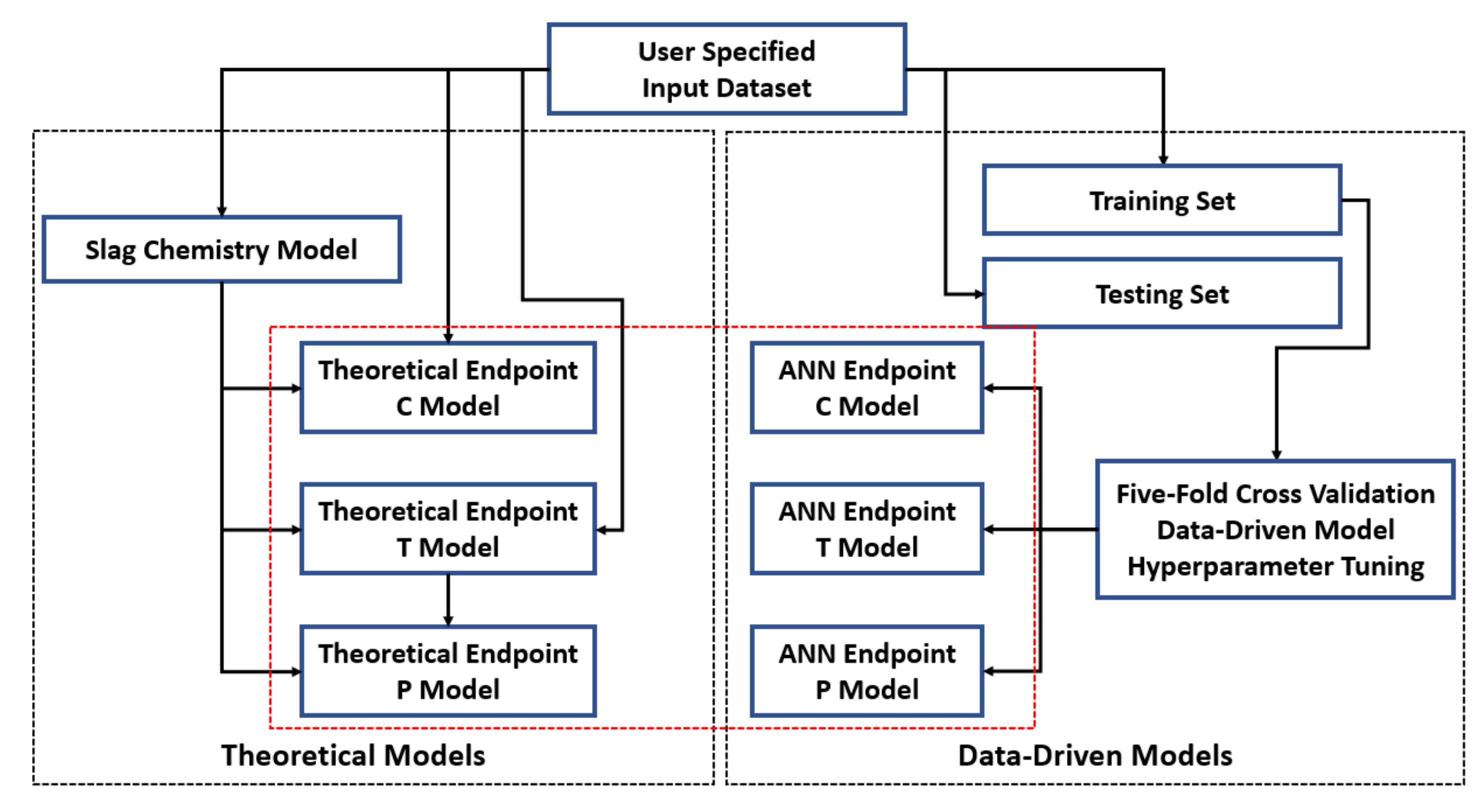
2.4. Hybrid Model Formulation

Much research has attempted to establish data-driven models for endpoint prediction by using various algorithms, such as radial basis function ANN, GMM, and TWSVM. These algorithms usually achieve a very high level of accuracy, but they are all plant-specific models and suffer from poor interpretability, which is a commonly known issue for machine learning techniques. The objective of the hybrid model development is to combine the advantages of both theoretical models and data-driven models and resolve their respective drawbacks. Therefore, a hybrid algorithm that contains a workflow combining a theoretical model and a machine learning model is proposed in this study.
The idea of the hybrid model formulation can be interpreted as an architecture that uses prediction from one model as the input variables for other models, where the exchange of input and output takes place. For example, turndown temperature is one of the key variables in predicting endpoint phosphorus by using thermodynamic driven equations. Thus, the predictive accuracy of the theoretical phosphorus model is expected to improve with the use of endpoint temperature with higher precision. The overall hybrid model consists of 7 models, as represented in Table 5.
In this study, all models were developed based on input parameters that are readily available in the beginning of the BOF process. As a result, variables such as slag chemistries cannot be directly used for fitting models. Due to this reason, the hybrid model started off by integrating the slag chemistry model (MM_S) with all theoretical models as shown in Figure 8a Once all theoretical models and ANN models are completed, the hybrid model continues with information exchange among individual models, as presented in Figure 8b. The numbers in Figure 8 represent the order of actions, which can be explained as the following:
  • User-specified inputs, such as hot metal chemistries, process parameters, and flux additions, were fed into the slag chemistry model. The results of “User Inputs” and “MM_S” corresponds to the input feature space that is used for model developments.
  • Theoretical models for endpoint carbon and temperature (MM_C and MM_T) were established by formulating mass and energy balance based on the input features from step 1.
  • Theoretical model for endpoint phosphorus (MM_P) was created based on slag chemistries from MM_S and endpoint temperature prediction from MM_T. Thermodynamic driven regression models [M1]–[M6] were tested against each other.
  • Three ANN networks were established by using user inputs, and hyperparameter tuning was conducted with five-fold cross-validation.
  • Endpoint carbon prediction from ANN_C was substituted as the endpoint carbon into MM_T to formulate mass balance. The assumption of using the median of endpoint carbon from dataset was discarded.
  • Since endpoint phosphorus is heavily dependent on turndown temperature, endpoint temperature prediction from ANN_T was substituted into MM_P and ANN_P.
  • Finally, endpoint phosphorus from ANN_P was substituted into MM_C and MM_T to complete the formulation of mass balance.
Figure 8. Overall schematic flow chart of hybrid model algorithm: (a) establish theoretical models and ANN models by using user inputs and slag chemistry models; (b) hybrid architecture consisting of theoretical models and ANN models.
Metals 12 00801 g008

3. Results

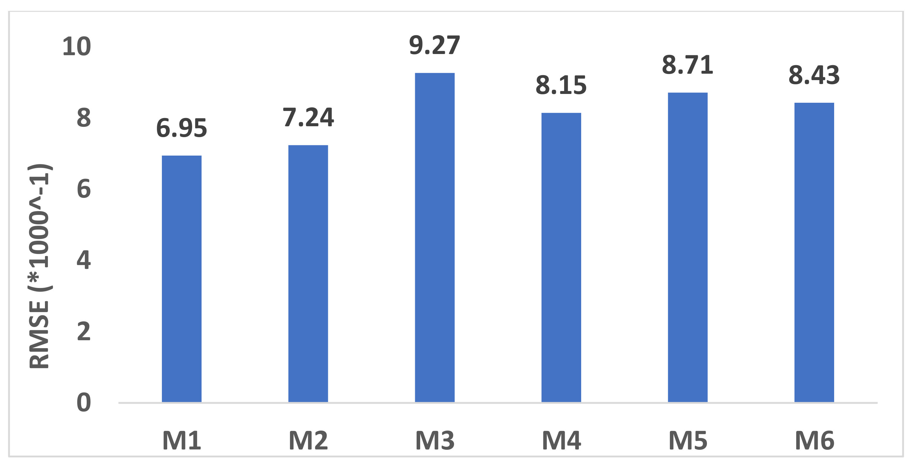
3.1. Theoretical Phosphorus Model Validation

As mentioned in Section 2, six regression-based models with thermodynamic principles were compared against each other to predict endpoint phosphorus content. RMSE was used as the evaluation metric for the predictive performance among each, and the results are displayed in Figure 9.
From Figure 9, [M1] achieves the lowest RMSE among all six models; thus, it is selected as the equation to be used in the theoretical endpoint phosphorus model (MM_P). To recall, [M1] is expressed as:
l p ^ = 0.431 % CaO / % SiO 2 0.361   log % MgO + 13590 Temp 5.71 + 0.384   log % Fe . total

3.2. Theoretical Model Results

The results of the predictive evaluation metrics for all three theoretical models are presented in Table 6. In this table, both RMSE and NRMSE values are provided for comparison. Among all three theoretical models, MM_C provides the best predictive performance with an NRMSE around 0.135, whereas MM_T gives out the highest NRMSE at 0.536.

3.3. ANN Model Hyperparamter Selection

For most machine learning models, the hyperparameters are parameters that cannot be derived through training. The hyperparameters are very important in that they control the learning process by means of factors such as learning time and convergence. These values are initialized by the user and tuned empirically. In this study, hyperparameters are tuned via a trial-and-error approach. For ANN models, the structure of the neural network, determined by number of neurons and layers, is usually the first hyperparameter to test out. In general, a neural network with only one hidden layer is named a single-layer neural network, and a neural network with more than one hidden layer is known as a multilayer perceptron. A single-layer neural network can be used to represent linearly separable functions, and a multilayer perceptron can be implemented to overcome the limitation of linear separability in high dimensional space. On the other hand, the batch size is a hyperparameter that controls the number of training examples in a single forward and backward propagation as described in Section 2. A large batch size can lead to degradation in the generalization of models, whereas a small batch size can take too long for the model to converge, which adversely affects the training time. Finally, the learning rate, a configurable hyperparameter, controls how quickly the ANN model adapts to the problem. A large learning rate can cause faster convergence outside of the global minimum solution, whereas a small learning rate can cause the model to get stuck in a local minimum. In this study, hyperparameters were selected based on trial and error, with the starting values, increments, and end values displayed in Table 7. For each model, the hyperparameters were selected based on the combination that achieves the lowest validation loss (RMSE).
In addition to the hyperparameters discussed in Table 7, the number of epochs is also a crucial hyperparameter for the training phase of ANN models. One epoch refers to a complete cycle through the entire training set, including forward pass and backpropagation. During the training phase of ANN models, the training set is split into training and validation sets, in which the training set is used for model fitting and the validation set for the purpose of testing. A typical trace of training and validation losses throughout all epochs for ANN models is represented in Figure 10. At the beginning of the training (at early epochs), the model started with large RMSE loss value, and it kept dropping and stabilized after a certain epoch number. In order to ensure convergence in solution and efficient computation, early stopping is deployed during the training of ANN models. An early stopping of 20 epochs is selected for model developments, so that the model completes the training phase when validation loss does not drop after 20 epochs.

3.4. ANN Model Results

Three ANN models were created by using their corresponding hyperparameters, mentioned in Table 7. The results of the ANN models developed, based on Tata Steel’s dataset, are presented in Table 8. Training and validation RMSE values were collected by using five-fold cross-validation. It can be observed that no overfitting is present because training and validation RMSE values are comparable with each other. Validation NRMSE was calculated and recorded for the comparison among all three models. To compare the results of ANN models with that of theoretical models in Table 6, it can be observed that ANNs for all endpoints improved by different extents, where ANN_T achieves the largest reduction in NRMSE by 60.6%.

3.5. Hybrid Model Results

With the hybrid model formulation, four out of six models receive updated input features, whereas the inputs for ANN_C and ANN_T do not change, according to Figure 8b. As a result, the hybrid algorithm does not affect predictions from them. However, for the other four models, as a result of the updated features and hybrid architecture, their endpoint predictions and accuracies will be different from before. The evaluation results of hybrid models are presented in Table 9. The term “With Hybrid” refers to the evaluation metric obtained after implementing the hybrid algorithm. From Table 9, all of the hybrid models show improvements in endpoint predictions, where hybrid MM_P attains the largest improvement of 11.98% reduction in NRMSE, followed by hybrid ANN_P and MM_C with 3.55% and 2.96% reductions in NRMSE, respectively.

4. Discussion and Interpretation of Results

In this section, the analysis of the results is discussed. Firstly, the performance of the hybrid model algorithm and its comparison with non-hybrid models is discussed, and secondly, the application of such an algorithm from an industrial perspective is explained.

4.1. Hybrid Model Algorithm Performance and Comparison

Before the implementation of the hybrid algorithm, the ANN models for all three endpoints outperformed theoretical models, by 59.9% for endpoint temperature, 4.4% for endpoint carbon, and 17.23% for endpoint phosphorus. A comparison summary among theoretical models, ANN models, and hybrid models is presented in Table 10. As mentioned before, the formulation of theoretical models is based on homogeneity of physiochemical reactions and slag compositions at equilibrium, which is unlikely to be achieved in BOF production, due to the nature of the multi-phase and multi-variate process. Mathematically, the neural network algorithm is capable of solving the complex nonlinearity between input features and endpoints. In addition to this reason, the formulation of heat and mass balance in this study involves a number of assumptions, as described in Section 2, because the availability of input parameters is solely based on user-specified inputs. The inaccuracies introduced due to these assumptions during the formulation of mass balance can be propagated into the heat balance model and cause deviation in endpoint predictions.
With regards to the implementation of the hybrid algorithm, it can be found that all four hybrid models achieved lower NRMSE values as shown in Figure 11. One of the reasons for the improvement in predictive performance is due to the reduction in number of assumptions involved for theoretical models. The implementations of the hybrid algorithm, endpoint carbon and phosphorus from ANN models can be substituted directly into the heat and mass balance formulation, and endpoint temperature can be directly used for endpoint phosphorus calculation in the theoretical model. As a result, hybrid theoretical models benefit from the computational power provided by ANN. The Hybrid MM_P model showed the largest improvement of 9.77% in prediction accuracy, followed by hybrid MM_C and ANN_P with decrease in NRMSE of 3.7% and 1.17%, respectively. The reduction in NRMSE for hybrid MM_T was the lowest among all hybrid models at a 1.12%.

4.2. Application of the Results and Models for Industry

From an industrial point of view, it is crucial to introduce data-driven techniques in predicting endpoints for the BOF process due to their predictive power. As mentioned in Section 1, the majority of the current mechanism static models in predicting endpoints are based on heat and mass formulation, or dynamic control models, such as the sub-lance system. The implementation of data-driven techniques, such as machine learning, is proven to significantly improve the endpoint temperature prediction over that offered by the theoretical models. However, one of the drawbacks of data-driven models is that they are highly dependent on process parameters, which make them plant-specific rather than universal. On the other hand, the heat and mass balance model can be used as a universal model because it is developed based on thermodynamic principles. The proposed hybrid model of theoretical framework coupled with machine learning techniques can effectively increase the prediction accuracy of mechanism models by reducing the number of assumptions and simplifications in mass and heat balance, and improve the interpretability, as well as generalization, of data-driven models. This model proved to work seamlessly with the Tata Steel’s dataset, which contains production details of 28,000 heats. The hybrid model provided optimal predictive performance when training data and features were provided, but it can also be used as a universal model because of the presence of a theoretical framework.

5. Conclusions

A hybrid algorithm, based on heat and mass balance and neural network modeling, is proposed in this paper. The model predicts numerical values of endpoint temperature, carbon, and phosphorus based on user-specified inputs, such as hot metal chemistries, process parameters, and flux additions. With superb computational power in modeling nonlinearity, ANN models show improvements in endpoints predictions, especially in endpoint temperature. All hybrid models are observed to benefit from the implementation of the hybrid algorithm because the number of assumptions in heat and mass balance formulation is significantly reduced. Results have shown that hybrid MM_P achieved a 9.77% reduction in NRMSE, followed by 3.7% decrease for hybrid MM_C, hybrid ANN_P and MM_T attain 1.17% and 1.12% drop in NRMSE, respectively.
Finally, one of the main considerations of this study towards industry is the application of the hybrid model. In this paper, all prediction models were developed based on user-specified inputs which allow the model to be executed before production. In addition, the hybrid model can exploit the computational power of data-driven techniques and the generalization of theoretical models, which allow it to be implemented in either plant-specific or universal settings.

Author Contributions

K.C. conceptualized the assessment of theoretical models and machine-learning techniques on endpoint data; R.W. and I.M. conceptualized the use of hybrid model algorithm; I.M., T.K.R. and P.G. provided the process expertise and acquired data from Tata Steel; R.W. performed formulation of mass and heat balance and neural network modeling on the data; K.C. and I.M. provided funding of the project; R.W. designed and developed the algorithms, as well as implemented in on Python; K.C. provided mentorship of the project; R.W. created the figures in the paper; R.W. and A.S. wrote the initial draft of the manuscript; R.W. and A.S. edited and critically reviewed the final manuscript. All authors have read and agreed to the published version of the manuscript.

Funding

This research was funded by R&D TATA STEEL, Jamshedpur India and NSERC Discovery Grant in Canada.

Institutional Review Board Statement

Not applicable.

Informed Consent Statement

Not applicable.

Data Availability Statement

In this section, please provide details regarding where data supporting reported results can be found, including links to publicly archived datasets analyzed or generated during the study. Please refer to suggested Data Availability Statements in section “MDPI Research Data Policies” at https://www.mdpi.com/ethics, accessed on 20 February 2022. You might choose to exclude this statement if the study did not report any data.

Acknowledgments

The authors would sincerely thank R&D TATA Steel, Jamshedpur, India for providing all the necessary support towards this study.

Conflicts of Interest

The authors declare no conflict of interest.

References

  1. Ghosh, A.; Chatterjee, A. Ironmaking and Steelmaking: Theory and Practice; PHI Leanring Private Limited: New Delhi, India, 2008. [Google Scholar]
  2. Wang, X.; Han, M.; Wang, J. Applying input variables selection technique on input weighted support vector machine modeling for BOF endpoint prediction. Eng. Appl. Artif. Intell. 2010, 23, 1012–1018. [Google Scholar] [CrossRef]
  3. Iron Ore Monthly Price—US Dollars per Dry Metric Ton. Available online: https://www.indexmundi.com/commodities/?commodity=iron-ore (accessed on 15 November 2021).
  4. Bloom, T.A.; Fosnacht, D.R.; Haezebrouck, D.M. Influence of phosphorus on the properties of sheet steel products and methods used to control steel phosphorus levels in steel product Manufacturing. Part I. Iron Steelmak. 1990, 17, 35–41. [Google Scholar]
  5. Han, M.; Liu, C. Endpoint prediction model for basic oxygen furnace steel-making based on membrane algorithm evolving extreme learning machine. Appl. Soft Comput. J. 2014, 19, 430–437. [Google Scholar] [CrossRef]
  6. Xu, L.F.; Li, W.; Zhang, M.; Xu, S.X.; Li, J. A model of basic oxygen furnace (BOF) end-point prediction based on spectrum information of the furnace flame with support vector machine (SVM). Opt.-Int. J. Light Electron Opt. 2011, 122, 594–598. [Google Scholar] [CrossRef]
  7. Xu, L.; Li, W.; Xu, S.; Li, J.; Wang, Y. A new spectral analysis technique used in converter steelmaking BOF endpoint control. Adv. Mater. Res. 2010, 139–141, 689–692. [Google Scholar] [CrossRef]
  8. Iida, Y.; Emoto, K.; Ogawa, M.; Masuda, Y.; Onishi, M.; Yamada, H. Fully Automatic Blowing Technique for Basic Oxygen Steelmaking Furnace. Trans. Iron Steel Inst. Jpn. 1984, 24, 540–546. [Google Scholar] [CrossRef]
  9. Li, S.; Wei, X.; Yu, L. Numerical simulation of off-gas formation during top-blown oxygen converter steelmaking. Fuel 2011, 90, 1350–1360. [Google Scholar] [CrossRef] [Green Version]
  10. Cunha, A.P.; Pacianotto, T.A.; Frattini Fileti, A.M. Steelmaking process: Neural models improve end-point predictions. Comput. Aided Chem. Eng. 2004, 18, 631–636. [Google Scholar] [CrossRef]
  11. Philbrook, W.O. Thermochemistry of oxygen steel. JOM 1958, 10, 477–482. [Google Scholar] [CrossRef]
  12. Slatosky, W.J. End point temperature control in LD steelmaking. JOM 1960, 12, 226–230. [Google Scholar] [CrossRef]
  13. Meyer, H.W.; Dukelow, D.A.; Fischer, M.M. Static and dynamic control of the basic oxygen process. JOM 1964, 16, 501–507. [Google Scholar] [CrossRef]
  14. Neto, L.C. End-Blow Model for Control of LD Converters and Statistic Analysis of Its Performance. Master’s Thesis, Federal University of Minas Gerais, Belo Horizonte, Brazil, 1981. [Google Scholar]
  15. Fruehan, R.; Fortini, O.; Paxton, H. Theoretical Minimum Energies to Produce Steel for Selected Conditions; USDOE Office of Industrial Technologies: Washington, DC, USA, March 2000; Available online: http://scholar.google.com/scholar?hl=en&btnG=Search&q=intitle:Theoretical+Minimum+Energies+To+Produce+Steel+for+Selected+Conditions#1 (accessed on 10 February 2022).
  16. Madhavan, N.; Brooks, G.A.; Rhamdhani, M.A.; Rout, B.K.; Overbosch, A. General heat balance for oxygen steelmaking. J. Iron Steel Res. Int. 2021, 28, 538–551. [Google Scholar] [CrossRef]
  17. Madhavan, N.; Brooks, G.A.; Rhamdhani, M.A.; Rout, B.K.; Overbosch, A. Application of mass and energy balance in oxygen steelmaking. Ironmak. Steelmak. 2021, 48, 995–1000. [Google Scholar] [CrossRef]
  18. Balajiva, K.; Quarrell, A.; Vajragupta, P. A laboratory investigation of the phosphorus reaction in the basic steelmaking process. J. Iron Steel Inst. 1946, 153, 115. [Google Scholar]
  19. Suito, H.; Inoue, R. Thermodynamic assesment of hot metal and steeel dephosphorization with MnO-containing BOF slags. ISIJ Int. 1995, 35, 258–265. [Google Scholar] [CrossRef] [Green Version]
  20. Healy, G. New look at phosphorus distribution. J. Iron Steel Inst. 1970, 208, 664–668. [Google Scholar]
  21. Ide, K.; Fruehan, R.J. Evaluation of phosphorus reaction equilibrium in steelmaking. Iron Steelmak. 2000, 27, 65–70. [Google Scholar]
  22. IKEDA, T.; MATSUO, T. The dephosphorization of hot metal outside the steelmaking furnace. Trans. Iron Steel Inst. Jpn. 1982, 22, 495–503. [Google Scholar] [CrossRef] [Green Version]
  23. Ito, Y.; Sato, S.; Kawachi, Y.; Tezuka, H. Dephosphorization in LD converter with low Si hot metal-develop of minimum slag practice. Tetsu-Hagane 1979, 63, S737. [Google Scholar]
  24. Kawai, Y.; Takahashi, I.; Miyashita, Y.; Tachibana, K. For dephosphorization equilibrium between slag and molten steel in the converter furnace. Tetsu-Hagane 1977, 63, S156. [Google Scholar]
  25. Sipos, K.; Alvez, E. Dephosphorization in BOF Steelmaking. In Proceedings of the Molten 2009: VIII International Conference on Molten Slags, Fluxes and Salts, Santiago, Chile, 18–21 January 2009; GECAMIN: Santiago, Chile, 2009; pp. 1023–1030. [Google Scholar]
  26. Lee, C.M.; Fruehan, R.J. Phosphorus equilibrium between hot metal and slag. Ironmak. Steelmak. 2005, 32, 503–508. [Google Scholar] [CrossRef]
  27. Ogawa, Y.; Yano, M.; Kitamura, S.; Hirata, H. Development of the continuous dephosphorization and decarburization process using BOF. Tetsu-Hagane 2001, 87, 21–28. [Google Scholar] [CrossRef] [Green Version]
  28. Sarkar, R.; Gupta, P.; Basu, S.; Ballal, N.B. Dynamic Modeling of LD Converter Steelmaking: Reaction Modeling Using Gibbs’ Free Energy Minimization. Metall. Mater. Trans. B Process Metall. Mater. Process. Sci. 2015, 46, 961–976. [Google Scholar] [CrossRef]
  29. Biswas, J.; Ghosh, S.; Ballal, N.B.; Basu, S. A Dynamic Mixed-Control Model for BOF Metal–Slag–Gas Reactions. Metall. Mater. Trans. B Process Metall. Mater. Process. Sci. 2021, 52, 1309–1321. [Google Scholar] [CrossRef]
  30. Barui, S.; Mukherjee, S.; Srivastavs, A.; Chattopadhyay, K. Understanding dephosphorization in basic oxygen furnaces (BOFs) Using Data-driven Modeling Techniques. Metals 2019, 9, 955. [Google Scholar] [CrossRef] [Green Version]
  31. Phull, J.; Egas, J.; Barui, S.; Mukherjee, S.; Chattopadhyay, K. An application of decision tree-based twin support vector machines to classify dephosphorization in bof steelmaking. Metals 2020, 10, 25. [Google Scholar] [CrossRef] [Green Version]
  32. Li, J.N.; Li, Y.; Liu, F.; Bie, S.P.; Tang, C.C.; Zhang, X.L. Modeling of BOF steelmaking based on the data-driven approach. Adv. Mater. Res. 2013, 818, 92–97. [Google Scholar] [CrossRef]
  33. Wang, H.; Cai, J.; Feng, K. Predicting the Endpoint Phosphorus Content of Molten Steel in BOF by Two-stage Hybrid Method. J. Iron Steel Res. Int. 2014, 21, 65–69. [Google Scholar] [CrossRef]
  34. Feng, K.; Xu, A.J.; He, D.F.; Yang, L. Case-based reasoning method based on mechanistic model correction for predicting endpoint sulphur content of molten iron in KR desulphurization. Ironmak. Steelmak. 2020, 47, 799–806. [Google Scholar] [CrossRef]
  35. Hu, Y.; Zheng, Z.; Yang, J. Application of data mining in BOF steelmaking endpoint control. Adv. Mater. Res. 2012, 402, 96–99. [Google Scholar] [CrossRef]
  36. Han, M.; Jiang, L. Endpoint prediction model of basic Oxygen furnace steelmaking based on PSO-ICA and RBF neural network. In Proceedings of the 2010 International Conference on Intelligent Control and Information Processing, Dalian, China, 13–15 August 2010; pp. 388–393. [Google Scholar] [CrossRef]
  37. Laha, D.; Ren, Y.; Suganthan, P.N. Modeling of steelmaking process with effective machine learning techniques. Expert Syst. Appl. 2015, 42, 4687–4696. [Google Scholar] [CrossRef]
  38. Rahnama, A.; Li, Z.; Sridhar, S. Machine learning-based prediction of a BOS reactor performance from operating parameters. Processes 2020, 8, 371. [Google Scholar] [CrossRef] [Green Version]
  39. Cai, B.Y.; Zhao, H.; Yue, Y.J. Research on the BOF steelmaking endpoint temperature prediction. In Proceedings of the 2011 International Conference on Mechatronic Science, Electric Engineering and Computer (MEC), Jilin, China, 19–22 August 2011; pp. 2278–2281. [Google Scholar] [CrossRef]
  40. Fruehan, R.J.; Matway, R.J. Optimization of post combustion in steelmaking. In Office of Scientific & Tefchnical Information Technical Reports; American Iron and Steel Institute: Washington, DC, USA, 2004. [Google Scholar]
  41. Chen, E.; Coley, K.S. Kinetic study of droplet swelling in BOF steelmaking. Ironmak. Steelmak. 2010, 37, 541–545. [Google Scholar] [CrossRef]
  42. Selin, R. Studies on the MgO solubility in complex steelmaking slags in equilibrium with liquid iron and distribution of phosphorus and vanadium between slag and metal at MgO saturation. In Proceedings of the 3rd International Conference on Molten Slags and Fluxes, Glasgow, UK, 27–29 June 1988; pp. 317–322. [Google Scholar]
  43. Schurmann, E.; Fischer, H. Effect of composition and temperature of metal and slag on the dephosphorization with lime-saturated oxidizing slags at 1600 and 1700C. Steel Res. 1991, 62, 303–313. [Google Scholar]
  44. Bergman, A.; Gustafsson, A. Use of optical basicity to calculate phosphorus and oxygen contents in molten iron. In Proceedings of the 3rd International Conference on Molten Slags and Fluxes1, Glasgow, UK, 27–29 June 1988; pp. 150–153. [Google Scholar]
Figure 1. Flowchart of the development for theoretical models and data-driven models, models highlighted in red correspond to the participants in hybrid algorithm.
Metals 12 00801 g001
Figure 2. Flowchart of the slag chemistry model.
Metals 12 00801 g002
Figure 3. Flowchart of the endpoint carbon theoretical model.
Metals 12 00801 g003
Figure 4. Flowchart of the endpoint temperature theoretical model.
Metals 12 00801 g004
Figure 5. Flowchart of the endpoint phosphorus theoretical model.
Metals 12 00801 g005
Figure 6. General structure of an artificial neural network with three input and hidden neurons.
Metals 12 00801 g006
Figure 7. Schematic diagram of five-fold cross-validation.
Metals 12 00801 g007
Figure 9. RMSE comparison among six phosphorus equations [M1] to [M6] in endpoint P prediction.
Metals 12 00801 g009
Figure 10. Training and validation losses during the throughout 100 epochs for ANN_T.
Metals 12 00801 g010
Figure 11. NRMSE comparison among non-hybrid and hybrid models.
Metals 12 00801 g011
Table 1. Descriptive statistics of features and endpoints for Tata Steel dataset.
Feature CategoryVariableMeanStandard
Deviation
EndpointsEndpoint T1649.122.2
Endpoint C0.0440.013
Endpoint P0.01630.006
Hot Metal ChemistriesHM C4.5560.066
HM P0.1760.015
HM S0.0230.018
HM Mn0.0430.006
HM Si0.6410.162
HM Ti0.0690.015
HM Cr0.0090.005
Flux AdditionsLime8.5071.345
Dolomite3.6560.698
Iron Ore6.5962.004
Scrap10.6066.616
Process ParametersHM Weight163.97.0
HM Temperature1362.131.8
Oxygen Volume7807.6408.9
Blow Duration17.851.66
Blow End to Turndown Start Duration3.521.91
Blow End to Tapping Start Duration8.477.63
Tapping Duration5.51.99
Table 2. User-specified inputs used for multiple linear regression to predict slag basicity.
Feature CategoryVariable
Hot Metal ChemistriesHM C
HM P
HM S
HM Mn
HM Si
Flux AdditionsLime
Dolomite
Iron Ore
Scrap
Table 3. Existing models to predict phosphorus partition ratio in steelmaking.
ModelEquation
M1
[41]
l p ^ = 0.431 % CaO / % SiO 2 0.361   log % MgO + 13590 Temp 5.71 + 0.384   log % Fe . total
M2
[30]
l p ^ = 5.89 log % CaO + 0.5   log % P 2 O 5 + 0.6 % MnO + 15340 Temp 18.542 + 2.5   log % Fe . total
M3
[42]
l p ^ = 5.6 log % CaO + 22350 Temp 21.876 + 2.5   log % Fe . total
M4
[43]
l p ^ = 0.6639 % CaO / % SiO 2 + 8198.1 Temp 3.113 + 0.3956   log % Fe . total + 0.2075   log % C
M5
[4]
l p ^ = 0.08 % CaO + 2.5   log % Fe . total + 22350 Temp 16.0
M6
[44]
l p ^ = 7 log % CaO + 2.5   log % Fe . total + 22350 Temp 24.0
Table 4. Features used for neural network modeling.
Feature CategoryFeature Name
Hot Metal ChemistriesHot Metal Carbon
Hot Metal Sulfur
Hot Metal Silicon
Hot Metal Manganese
Hot Metal Phosphorus
Hot Metal Chromium
Hot Metal Titanium
Process ParametersOxygen Blow Duration
Blow End to Turndown Start Duration
Blow End to Tapping Start Duration
Tapping Duration
Blowing Strategy
Injected Oxygen Volume
Hot Metal Weight
Hot Metal temperature
Flux AdditionsLimestone
Dolomite
Iron Ore
Scrap
Table 5. Single models that are included in the hybrid model architecture.
Model TypePredicted EndpointAbbreviation
Theoretical ModelsSlag ChemistriesMM_S
Endpoint TemperatureMM_T
Endpoint CarbonMM_C
Endpoint PhosphorusMM_P
Data-Driven Technique
(ANN)
Endpoint TemperatureANN_T
Endpoint CarbonANN_C
Endpoint PhosphorusANN_P
Table 6. Model evaluations of the theoretical models for endpoint temperature, carbon, and phosphorus.
Model NameMM_TMM_CMM_P
RMSE53.580.01350.00695
Range of Endpoint1000.10.032
Normalized RMSE0.5360.1350.217
Table 7. Selection of hyperparameters for ANN model for all endpoints.
HyperparametersStarting ValueIncrementEnd ValueSelected Parameter
ANN_TANN_CANN_P
Number of Neurons161664323232
Number of Layers113222
Batch Size161664326432
Learning Rate0.0050.0050.020.010.0050.005
Table 8. Model evaluations of the ANN models for endpoint temperature, carbon, and phosphorus.
Model NameANN_TANN_CANN_P
Training RMSE21.360.01270.00553
Validation RMSE21.490.01290.00575
Validation NRMSE0.2150.1290.1796
Table 9. Comparison of model evaluations of the hybrid models and non-hybrid models.
Model NameMM_TMM_CMM_PANN_P
RMSE53.070.01300.00630.005680
NRMSE
(With Hybrid)
0.5310.1300.1960.1775
NRMSE
(Without Hybrid)
0.5360.1350.2170.1796
Improvement1.12%3.7%9.77%1.17%
Table 10. Model evaluations of the hybrid models and non-hybrid models.
Model NameMM_TMM_CMM_PANN_PANN_TANN_C
NRMSE
(With Hybrid)
0.5310.1300.1960.17750.2150.129
NRMSE
(Without Hybrid)
0.5360.1350.2170.1796//
Improvement1.12%3.7%9.77%1.17%//
Publisher’s Note: MDPI stays neutral with regard to jurisdictional claims in published maps and institutional affiliations.

