Evaluation on Flexibility of Phenomenological Hardening Law for Automotive Sheet Metals

Abstract

Constitutive modeling of sheet metals involves building a system of equations governing the material behavior under multi-axial stress states. In general, these equations require a hardening law that describes the stress-strain relationship. This study provides a thorough examination of the existing phenomenological hardening laws in the literature. Based on their ordinary differential equations, special efforts were made to discuss the degree of flexibility of these hardening laws. Four new phenomenological hardening laws were proposed during the discussions to capture the stress-strain relationship of automotive sheet metals, such as aluminum alloy and steel sheets. Then, applications of 18 hardening laws for fitting the uniaxial tensile stress-strain data of 12 automotive sheet metals were thoroughly compared. The comparisons reveal that the proposed hardening laws capture well the experimental stress strain data of all examined materials. Compared to several combined hardening laws, the proposed functions have comparable flexibility but require fewer parameters.

1. Introduction

Sheet metals are widely used in different industrial applications: automotive, aerospace, ocean, and building engineering [1,2]. However, due to the nature of material anisotropy and non-proportional loadings, computational modeling of sheet metal behaviors subjected to a forming process is a difficult task [3]. As a result, the creation of new material models is critical to the success of sheet metal modeling.

According to the scale of their application, computational models of sheet metals can be classified into macroscopic and microscopic models [4,5]. The former takes into account the experimental phenomena observed during deformation processes and attempts to simplify the material’s behavior as much as possible. Consequently, these models are appropriate for simulating and analyzing sheet metal forming processes of large-size parts. Microscopic models, on the other hand, are widely developed based on physical insights from material sciences, such as dislocation and grain boundary interactions associated with crystal plasticity theories. More detail is used in the description of material behavior under generalized external loads in this approach. Both modeling approaches necessitate three components: a hardening law, a yield function, and a flow rule. The purpose of this research is to characterize and discover the formulation of macroscopic hardening laws for automotive sheet metals.

A large number of macroscopic hardening laws have been proposed to describe the behavior of sheet metals [6]. Generally, they reproduce the experimental stress-strain relationship following either saturation laws or power laws. Myriad steel and aluminum alloy sheets have applications in the vast majority of automotive sheet metals. For example, Figure 1 depicts the use of common hardening laws, such as the Voce [7], Hockett–Sherby [8], Hollomon [9], and Swift [10] models, in capturing the stress-strain data obtained from a standard uniaxial tensile (UT) test of AA6016-T4 sheets, of which the experimental stress-strain data were reported in a previous study [11]. It can be seen that all of the models under consideration provide excellent matches with the experimental data. Their extrapolations to larger strain ranges, however, show significant discrepancies. The inconsistency of their extrapolations is well-known in the literature and raises a specific care for modelers in selecting a proper hardening law for a typical tested material.

Numerically, their deviation is originated from the formulation of each hardening law, as well as the identified parameters. Considering the evolution of hardening rate according to the flow stress explores the reason for the deviation [12]. According to Figure 1b, the Voce model uses a linear plot to approximate the hardening rate curve, which appears to underestimate the material behavior in the extrapolation ranges. Other models, such as Hollomon, Swift, and Hockett–Sherby, produce similar estimates for the evolution of the hardening rate in a flow stress range of 300–350 MPa. Thus, as shown in Figure 1a, their predictions for the post-necking behavior of the investigated material are more similar. Therefore, an ordinary differential equation (ODE) can be used to evaluate the formulation of a hardening law by describing the relationship between the hardening rate and the flow stress.

The objective of this study is twofold. First, the ODE of common hardening laws for automotive sheet metals is summarized. Detailed discussions on the formulation of their ODE are provided. Second, four new hardening models are proposed based on these discussions to capture the stress-strain relationship of sheet metals. The proposed models are formulated under the assumption that they compound four parameters. The proposal of new functions aims to enrich the set of constitutive equations for sheet metals. The rest of the paper is structured as follows. Section 2 delineates the ODE of 14 hardening models divided into three categories: saturation laws, power laws, and combinations. The formulation of newly proposed hardening laws is presented in detail in Section 3. Section 4 compares applications of 18 mentioned hardening laws in reproducing the stress-strain data of 12 automotive sheet metals (six steel and six aluminum alloy sheets). Section 5 validates the usefulness of the identified proposed hardening laws in simulating the UT tests for all investigated materials. Section 6 summarizes and discusses the work’s perspectives and limitations.

2. Ordinary Differential Equation of Existing Hardening Laws

An overview of various existing phenomenological hardening laws in the literature is presented in detail, focusing on their ODE formulations. The models could be classified into three groups: saturation laws, power laws, and combinations. Hereafter, $H\left(\overline{\epsilon }\right)$ denotes a hardening function of the equivalent plastic strain $\overline{\epsilon }$, and $H\prime$ denotes its derivative or the hardening rate function; $c_i$ denote parameters of the hardening law, which should be determined for any investigated material.

2.1. Saturation Laws

Saturation laws impose saturated stress at large strains. The hardening law proposed by Voce [7] is the most common form in this group, of which the formulation is expressed in Equation (1a). The model’s spread is due to its simplicity [6,13,14,15]. As shown in Equation (1b), the work-hardening rate predicted by this model can be expressed by a first-order linear ODE. The formulation results in a linear approximation of the hardening rate based on flow stresses, as shown in Figure 1b. Although the model provides a good estimation for the experimental stress-strain data obtained from the UT test, there is a clear discrepancy between the model estimation and the experimental data, especially near the end of the experimental data. Moreover, the deformation observed during the UT test is relatively small compared to those examined in industrial forming processes [16,17,18]. Therefore, premature failure prediction of the hardening law is noticed for several forming processes [19,20].

Voce:

$$H\left(\overline{\epsilon }\right)=c_1-c_2\exp \left(-c_3\overline{\epsilon }\right)$$

(1a)

$$H^{\prime }=\left(c_1-H\right)c_3$$

(1b)

Hockett and Sherby [8] performed compression tests for polycrystalline solids (alpha Uranium and iron) to characterize the stress-strain relationship of the investigated material at large strains. They proposed a hardening law to describe the derived experimental data (Equation (2a)). Based on log-scale plots of experimental data, they recommended a value of 0.58 for parameter c₄ for all examined materials in their study, which led to excellent estimation for all tested materials, particularly in large strain ranges. However, other values of parameter c₄ can be used for different materials (see the Supplementary Material).

Hockett–Sherby:

$$H\left(\overline{\epsilon }\right)=c_1-c_2\exp \left(-c_3{\overline{\epsilon }}^{c_4}\right)$$

(2a)

$$H^{\prime }=\left(c_1-H\right)c_3{c}_4{\overline{\epsilon }}^{(c_4-1)}$$

(2b)

Later, Chinh et al. [21] conducted a series of experimental tests for polycrystalline aluminum and copper to explore the stress-strain relationship in wide strain ranges. Their experimental results demonstrated that the macroscopic flow curves follow a power law in small strain ranges and become saturated in large strain ranges. As a result, they proposed an exponential-power law for the stress-strain relationship, as shown in Equation (3a). In fact, the proposed hardening law is consistent with the one proposed by Hockett and Sherby [8], as evidenced by their ODEs (Equations (2b) and (3b)). In these equations, a multiplication of a constant ($c_3$ in Equation (2b) and $\frac{1}{c_3}$ in Equation (3b)) with a strictly decreasing function $c_4{\overline{\epsilon }}^{(c_4-1)}$ produces a nonlinear evolution of the hardening rate.

Chinh et al.:

$$H\left(\overline{\epsilon }\right)=c_1-c_2\exp \left(-\frac{{\overline{\epsilon }}^{c_4}}{c_3}\right)$$

(3a)

$$H^{\prime }=\left(c_1-H\right)\frac{c_4{\overline{\epsilon }}^{(c_4-1)}}{c_3}$$

(3b)

2.2. Power Laws

As opposed to the saturation laws, power hardening laws present unbounded stresses at large strains. The simplest power hardening law was proposed by Hollomon [9] with two parameters, as shown in Equation (4a). Ludwik [22] pioneered the use of another power law to describe the stress-strain relationship, as expressed in Equation (5a). Furthermore, Swift’s [10] power hardening law is widely used to describe the flow curve of steels and irons [20,23,24]. The power laws construct strictly increasing functions of the flow curve. Consequently, their hardening rate functions are always positive because they are carried out using reciprocal functions. With only two parameters, the Hollomon model has some practical limitations. Both the Ludwik and Swift models contain three parameters, but the latter seems to be more flexible than the former, according to their ODE.

Hollomon:

$$H\left(\overline{\epsilon }\right)=c_1{\overline{\epsilon }}^{c_2}$$

(4a)

$$H^{\prime }=H\frac{c_2}{\overline{\epsilon }}$$

(4b)

Ludwik:

$$H\left(\overline{\epsilon }\right)=c_1+c_2{\overline{\epsilon }}^{c_3}$$

(5a)

$$H^{\prime }=\left(H-c_1\right)\frac{c_3}{\overline{\epsilon }}$$

(5b)

Swift:

$$H\left(\overline{\epsilon }\right)=c_1{\left(\overline{\epsilon }+c_2\right)}^{c_3}$$

(6a)

$$H^{\prime }=H\frac{c_3}{\overline{\epsilon }+c_2}$$

(6b)

Both saturation and power hardening laws are widely used to practically describe the hardening behavior of sheet metals. The limitation of these hardening laws is their inflexibility in capturing the flow curve over wide strain ranges [14,23,25]. The limitation can be deduced mathematically from the formulations of their ODEs, which contain two or three parameters. As a result, their approximations for hardening rate curves frequently deviate from the experimental data (see Figure 1b), particularly at the two ends of the data sequence. Therefore, numerous combinations of these hardening laws have been introduced in the literature to improve the flexibility of the imposed hardening law.

2.3. Combination of Hardening Laws

Combining two or more functions in one hardening law will increase its flexibility. However, the act also increases the number of hardening law parameters, which may make calibrating their values more difficult. The following sections go over the two most common methods for establishing a combined hardening law: additive formulation and multiplicative formulation.

2.3.1. Additive Combination

Conventionally, the stress-strain data obtained from a standard UT test are used to identify parameters of a selected hardening law by a curve fitting method. For various automotive sheet metals, the fitting method typically provides a good enough approximation for the available data, either using saturation laws or power laws. Their extrapolations to larger strain ranges, however, show significant discrepancies. As a result, a linear combination of a power law and a saturation law in an additive form [26,27,28,29], as expressed in Equation (7a), can be used for intermediate extrapolations over a wider strain range. At the same time, the combination maintains the same order of accuracy in their approximations for the fitting range. In Equation (7a), H₁ denotes a power hardening law that could be the Hollomon, Ludwik, or Swift models, while H₂ denotes a saturation hardening law in form of Voce or Hockett–Sherby models; $c_1$ is a linear combined factor ($0<c_1<1$). Equation (7b) also includes an ODE formulation of the corresponding hardening rate. As an example, Figure 2 shows an application of a linear combination of the Swift and Voce models (LSV model) with $c_{1 }=0.7$ on modeling the stress-strain data of AA6016-T4 sheets. It is worth noticing that H₁ and H₂ are both excellent approximations for the experimental data. As a result, the first term of Equation (7b) yields an average of the two functions over the entire strain range, as illustrated in Figure 2. The second term, on the other hand, involves their difference, which primarily contributes to the extrapolation ranges.

Hollomon/Voce; Swift/Voce; Swift/Hockett–Sherby:

$$H\left(\overline{\epsilon }\right)=c_1{H}_1+\left(1-c_1\right)H_2$$

(7a)

$$H^{\prime }=\frac{1}{2}\left(H_1^{\prime }+H_2^{\prime }\right)+\left(c_1-\frac{1}{2}\right)\left(H_1^{\prime }-H_2^{\prime }\right)$$

(7b)

As alternatives to the above-mentioned method, several additive combinations of two single functions have been introduced in the literature. For example, Kim et al. [14] modified a Voce hardening law by adding a linear term. The same approach was applied to modify the Hockett–Sherby model [30,31]. Besides, Koc and Štok [32] introduced a double Voce function to improve the simulation results of an austenitic stainless steel coupon subjected to a standard UT test. Furthermore, Ludwigson [33] proposed a modified Hollomon model by including an exponential term, which was shown to improve the hardening law’s accuracy at low strains [34]. In addition, Lavakumar et al. [35] proposed adding one more exponential term to Ludwigson’s model to improve the accuracy of the derived flow curve at large strains. The ODE of these hardening laws, like the previous additive approach, can be separated into different terms. The first term overall averages the contributions of the involved functions, while the others characterize their compensated effects at different strain ranges. Thus, the more additive terms are used, the more a flexibility of the hardening law is achieved.

Modified Voce:

$$H\left(\overline{\epsilon }\right)=c_1-c_{2}exp\left(-c_3\overline{\epsilon }\right)+c_4\overline{\epsilon }$$

(8a)

$$H^{\prime }=\frac{1}{2}\left(c_1-H\right)\left(c_3+\frac{1}{\overline{\epsilon } }\right)+\frac{1}{2}\left(c_4-\frac{1}{\overline{\epsilon }}\right)\left(c_2\exp \left(-c_3\overline{\epsilon }\right)+c_4\overline{\epsilon }\right)$$

(8b)

Double Voce:

$$H\left(\overline{\epsilon }\right)=c_1-c_{2}exp\left(-c_3\overline{\epsilon }\right)-c_{4}exp\left(-c_5\overline{\epsilon }\right)$$

(9a)

$$H^{\prime }=\frac{1}{2}\left(c_1-H\right)\left(c_2+c_4\right)+\frac{1}{2}\left(c_2+c_4\right)\left(c_{2}exp\left(-c_3\overline{\epsilon }\right)-c_{4}exp\left(-c_5\overline{\epsilon }\right)\right)$$

(9b)

Ludwigson:

$$H\left(\overline{\epsilon }\right)=c_1{\overline{\epsilon }}^{c_2}+\exp \left(c_3+c_4\overline{\epsilon }\right)$$

(10a)

$$H^{\prime }=\frac{1}{2}H\left(\frac{c_2}{\overline{\epsilon } }+c_4\right)+\frac{1}{2}\left(\frac{c_2}{\overline{\epsilon } }-c_4\right)\left(c_1{\overline{\epsilon }}^{c_2}-\exp \left(c_3+c_4\overline{\epsilon }\right)\right)$$

(10b)

2.3.2. Multiplicative Combination

Besides the spreading of additive combined hardening laws, several hardening laws were constructed by multiplying two or more functions together. One of these functions is the Misiolek equation [6], which is a product of a Hollomon power law and an exponential function, as expressed in Equation (11a). The equation was used to explain the flow curve of various sheet materials [36,37]. In comparison to the Hollomon equation, the ODE of the Misiolek model has one more parameter that increases its flexibility.

Misiolek:

$$H\left(\overline{\epsilon }\right)=c_1{\overline{\epsilon }}^{c_2}\exp \left(c_3\overline{\epsilon }\right)$$

(11a)

$$H^{\prime }=H\left(\frac{c_2}{\overline{\epsilon }}+c_3\right)$$

(11b)

Recently, Pham and Kim [38] proposed another multiplicative combination of hardening laws for which the formulations of the flow stress and hardening rate were expressed as:

Pham and Kim:

$$H\left(\overline{\epsilon }\right)=c_1+c_2\left[\left(1-\exp \left(-c_3\overline{\epsilon }\right)\right]{\left(\overline{\epsilon }+0.002\right)}^{c_4}\right],$$

(12a)

$$H^{\prime }=\left(H-c_1\right)\left(\frac{c_3}{\exp \left(c_3\overline{\epsilon }\right)-1}+\frac{c_4}{\overline{\epsilon }+0.002}\right).$$

(12b)

The ODE of this model contains three adjustable parameters, that may increase its flexibility. Previous studies demonstrated the good capacity of this model in predicting the hardening behavior of several aluminum alloy sheets [11,39] and steels [40,41].

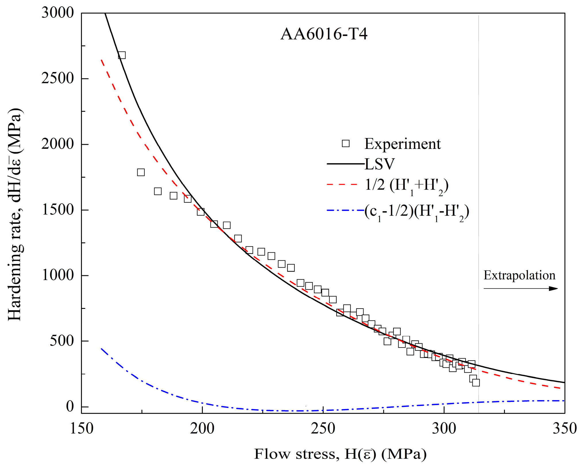
3. New Strain Hardening Law

Literature reviews indicated that there does not exist a hardening law that is suitable for all kinds of automotive sheet metals. The need to investigate new hardening laws to broaden the set of constitutive models is critical to the success of simulating the forming processes of newly developed materials. A new hardening law should be very flexible to have a wide range of practical applications. However, the number of parameters involved should be kept to a minimum to simplify the calibration process. Thus, only four-parameter hardening laws are considered in this section for the sake of simplicity.

3.1. Saturation Law

Comparing Equations (1b) and (2b) reveals the significance of parameter $c_4$ in the Hockett–Sherby model. The term $c_4{\overline{\epsilon }}^{(c_4-1)}$ in Equation (2b) is reduced to a negative exponent function if $c_4<1$. Therefore, a new hardening law is proposed (named Proposed 1), of which the ODE is regulated by a reciprocal function as follows:

Proposed 1:

$$H\left(\overline{\epsilon }\right)=c_1-c_2{\left(\overline{\epsilon }+c_3\right)}^{(-c_4)}$$

(13a)

$$H^{\prime }=\left(c_1-H\right)\frac{c_4}{\overline{\epsilon }+c_3}$$

(13b)

This formulation is similar to the one suggested by Sahoo et al. [42], which was proposed based on observations with crystal plasticity. However, different methods should be used to identify parameters of these models that may affect the predictive capacity of the calibrated hardening law [42].

Alternatively, Equation (12b) requires two terms, $\frac{c_3}{exp\left(c_3\overline{\epsilon }\right)-1}$ and $\frac{c_4}{\overline{\epsilon }+0.002}$, to procreate a combination. One may average their contributions by simplifying to a single function as:

Proposed 2:

$$H\left(\overline{\epsilon }\right)=c_1+c_2{\left[1-\exp \left(-c_3 \overline{\epsilon }\right)\right]}^{c_4}$$

(14a)

$$H^{\prime }=\left(H-c_1\right)\frac{c_3}{\exp \left(c_3\overline{\epsilon }\right)-1}$$

(14b)

This proposed formulation is similar to the Sellars’s model [6] but requires one more parameter for increasing its flexibility.

3.2. Power Law

Practically, power hardening laws do not restrict the upper bound of the flow stress because of their power coefficient. A generic four-parameter power hardening law can be expressed as:

$$H\left(\overline{\epsilon }\right)=c_1{\left(g\left(\overline{\epsilon }\right)\right)}^{c_4}$$

(15)

where $g\left(\overline{\epsilon }\right)$ is a two-parameter function of $\overline{\epsilon }$. Mathematically, the ODE of this equation can be expressed as:

$$H^{\prime }=H{c}_4\frac{g\prime \left(\overline{\epsilon }\right)}{g\left(\overline{\epsilon }\right)}$$

(16)

Numerically, $g\left(\overline{\epsilon }\right)$ can be an arbitrary of which the term $\frac{g\prime \left(\overline{\epsilon }\right)}{g\left(\overline{\epsilon }\right)}$ should be a strictly decreasing and non-negative function. For example, $g\left(\overline{\epsilon }\right)$ of the Swift model is a modification of the identity function, which is mathematically equivalent to a linear function. Therefore, this study imposes a modified Sigmoid function to $g\left(\overline{\epsilon }\right)$ leading to the following hardening law:

Proposed 3:

$$H\left(\overline{\epsilon }\right)=c_1{\left(1+\frac{c_2\overline{\epsilon }}{{\left[1+{\left(c_2\overline{\epsilon }\right)}^{c_3}\right]}^{1/c_3}}\right)}^{c_4}$$

(17a)

$$H^{\prime }=H{c}_4\frac{c_2}{[c_2\overline{\epsilon }+{\left(1+{\left(c_2\overline{\epsilon }\right)}^{c_3}\right)}^{1/c_3}]\left(1+{\left(c_2\overline{\epsilon }\right)}^{c_3}\right)}$$

(17b)

In another way, the nonlinearity of $g\left(\overline{\epsilon }\right)$ is secured by adding an exponential function to a linear term as follows:

Proposed 4:

$$H\left(\overline{\epsilon }\right)=c_1{\left(2-\exp \left(-c_2\overline{\epsilon }\right)+c_3\overline{\epsilon }\right)}^{c_4}$$

(18a)

$$H^{\prime }=H{c}_4\frac{c_2\exp \left(-c_2\overline{\epsilon }\right)+c_3}{2-\exp \left(-c_2\overline{\epsilon }\right)+c_3\overline{\epsilon }}$$

(18b)

Compared to formulations of the common hardening laws presented in the previous section, the proposed hardening laws adjust their ODE aiming to increase the flexibility of the derived functions. Therefore, they may have better flexibility than the well-known hardening laws, such as the Voce, Hockett–Sherby, Hollomon, and Swift models and require fewer parameters than their combinations. Applications of the proposed hardening laws are discussed in the next section.

4. Application for Automotive Sheet Metals

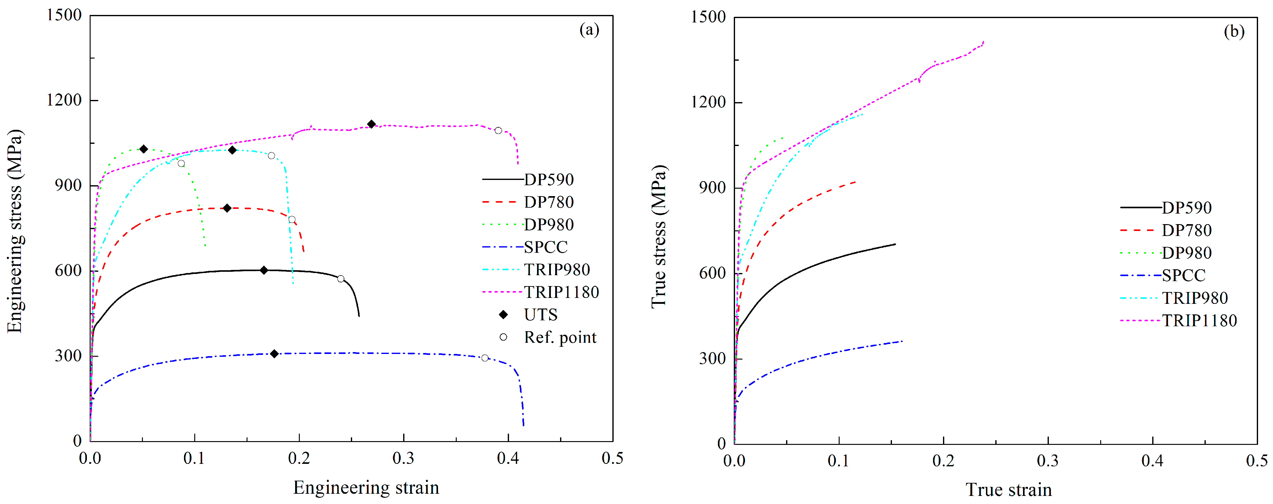
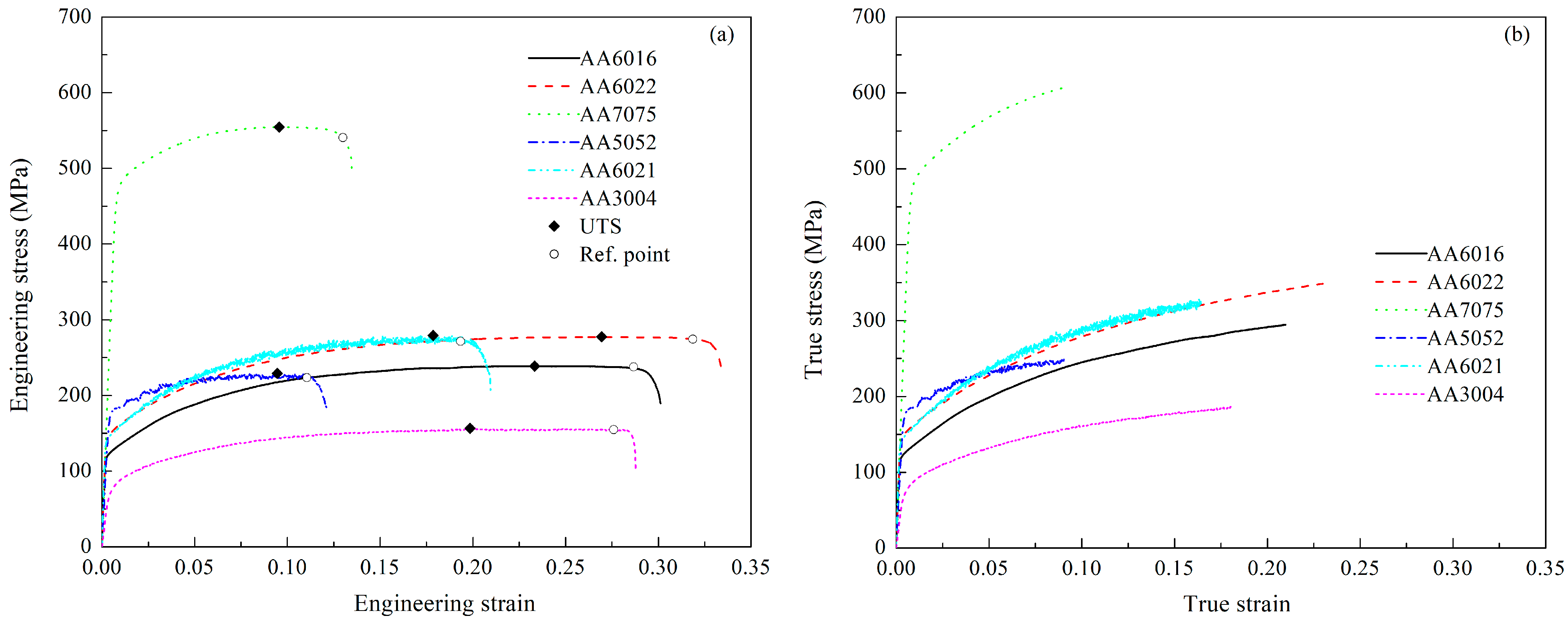
4.1. Investigated Materials

Six steel (DP590, DP780, DP980, SPCC, TRIP980, and TRIP1180) and six aluminum alloy (AA6016, AA6022, AA7075, AA5052, AA6021, and AA3004) sheets, which are widely used in automotive industries, are investigated in this study. The investigated materials were subjected to uniaxial tensile tests following the Korean standard KS B0810-13B [43]. The specimens were all prepared in the rolling direction.

Table 1. Material properties were obtained from the uniaxial tensile test of the investigated materials.

Material	Thickness (mm)	Young Modulus (GPa)	Initial Yield Stress (MPa)	Ultimate Tensile Strength (MPa)	Maximum Uniform Strain	Elongation (%)
DP590	1.4	205	401	603	0.156	25.7
DP780	1.2	206	489	822	0.123	20.5
DP980	1.6	200	800	1030	0.050	11.0
SPCC	0.9	210	158	309	0.158	41.4
TRIP980	1.2	213	640	1026	0.120	19.5
TRIP1180	1.25	207	854	1117	0.229	40.9
AA6016	1.2	69	158	277	0.238	33.4
AA6022	1.1	67	123	238	0.209	30.1
AA7075	1.6	67	478	554	0.091	13.5
AA5052	0.8	73	173	229	0.090	12.2
AA6021	1.4	71	146	279	0.157	20.9
AA3004	0.51	62	73	156	0.171	28.7

summarizes the material properties obtained from the tests. Furthermore, the experimental stress-strain data of steel and aluminum sheets are shown in Figure 3 and Figure 4 respectively. Although the heat treatments are important to the hardening behavior of aluminum sheets, their effects on the derived stress-strain data are out of the scope of this study. Thus, the heat treatment conditions applied to the examined aluminum are not specified in what follows.

It is seen that the variation of the Young modulus of steel sheets determined from the tests is negligible, which is close to a value of 200 GPa, approximately. The measured Young modulus of aluminum alloy sheets, which is approximated to 70 GPa, yielded similar results. However, the plastic properties of these materials vary greatly from one another. For example, initial yield stresses of steel sheets range from 150 MPa (SPCC) to 1000 MPa (DP980 and TRIP980). The shortest elongation of 10% was observed in the case of the DP980 sheet, whereas, the longest elongation is the more than 40% observed in the case of the TRIP1180.

Furthermore, the ultimate tensile strengths (UTS) of the tested materials are marked in Figure 3 and Figure 4 to indicate the ranges of uniform deformations observed during the UT tests. It is well-known that necking begins beyond the points, resulting in inhomogeneous deformations. Hence, the deformation is concentrated on a narrow regime, subsequently leading to the strain localization. Once the strain localization is formed, the failure occurs quickly. In these figures, reference points are depicted to indicate the position of strain localization observed during the tests for each material. These reference points were determined based on the authors’ expertise since there is no standard for detecting the strain localization on the engineering stress-strain data. It is recommended to extract the reference point to match a requirement that the engineering stress is more than 95% of UTS [41]. Some materials, such as DP980, AA5052, and AA6021, fail shortly after the initiation of the diffuse neck. However, some materials, such as SPCC, TRIP1180, AA6022, and AA3004, exhibit a wide deformation range after UTS. The observation demonstrates various degrees of ductility of the tested materials. Consequently, capturing the behaviors observed during the tensile tests for all investigated materials requires the use of a high-flexibility hardening law.

4.2. Calibration Method

The true stress-strain data obtained from the UT tests are used to identify parameters of the before-mentioned hardening laws. For this purpose, the common and constrained curve fitting methods [44] are detailed in the next subsection.

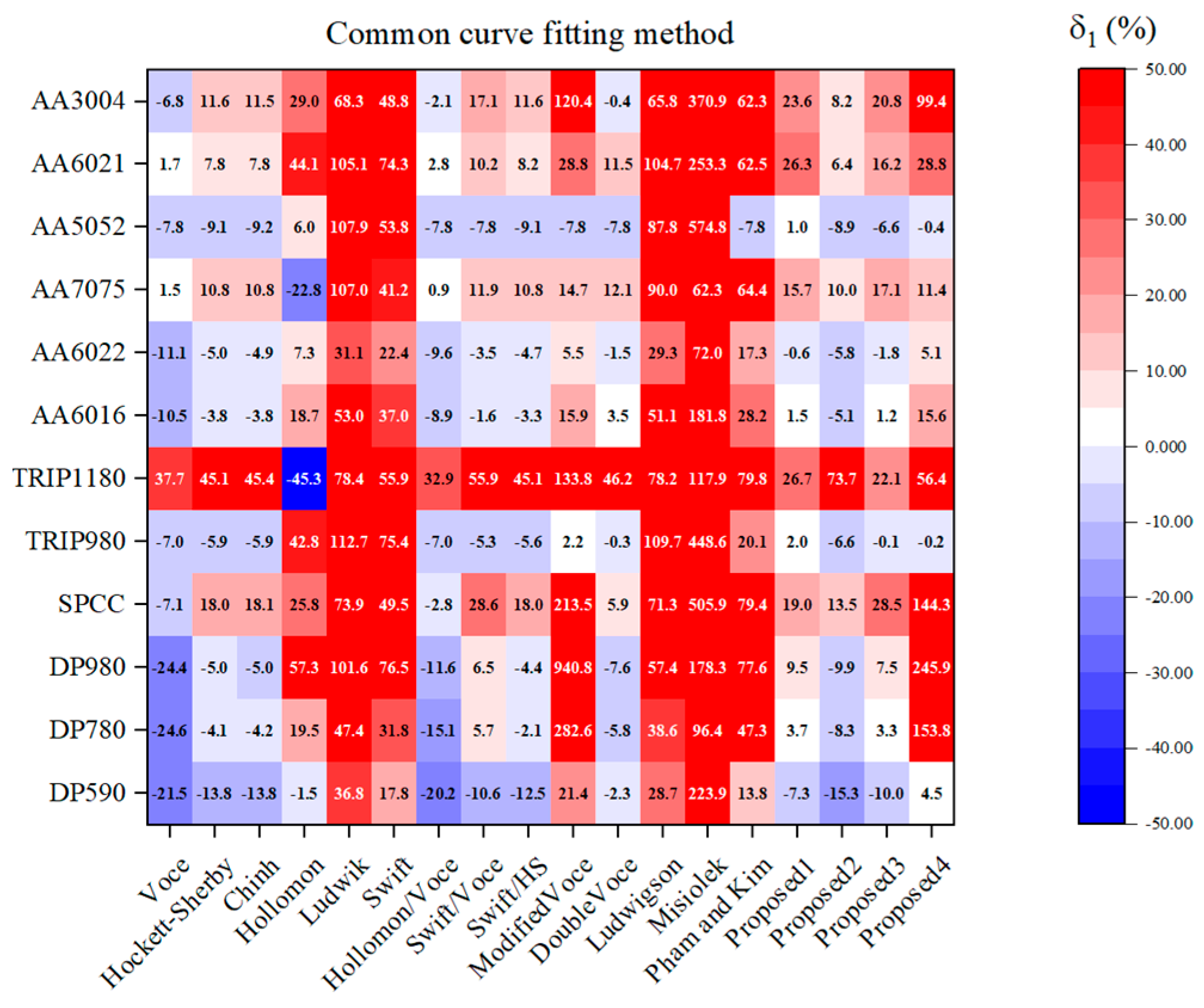
4.2.1. Common Curve Fitting Method

In this method, a cost function of root mean square error (RMSE) is constructed as follows:

$$RMSE=\sqrt{{\displaystyle \sum }_{i=1}^N{\left(H\left({\overline{\epsilon }}_i\right)-{\sigma }_i\right)}^2}$$

(19)

where ${\overline{\epsilon }}_i$ and ${\sigma }_i$ denote the measured stress-strain data obtained from an experimental test; N denotes the number of experimentally measured points. Then, a generalized reduced gradient algorithm is applied to minimize the cost function by using a Python script developed by the authors.

4.2.2. Constrained Curve Fitting Method

A previous study pointed out the link between the accuracy of a hardening law’s prediction for ${\epsilon }_u^{*}$ and its usefulness in estimating the forming limit curve (FLC) of sheet metals [11,44]. Pham et al. [11] suggested increasing the weight factor of the points surrounding ${\epsilon }_u^{*}$ in the fitting routine. Furthermore, Noder and Butcher [44] proposed enforcing the maximum force criterion as a constraint of the fitting procedure. The constraint is expressed as follows:

$$\frac{H\prime \left({\epsilon }_u^{*}\right)}{H\left({\epsilon }_u^{*}\right)}=1$$

(20)

The before-mentioned calibration methods are applied to identify parameters of 18 hardening laws for 12 examined materials. The application of the common curve fitting method is straightforward. In the constrained curve fitting method, the value of ${\epsilon }_u^{*}$ for each material is determined from its maximum uniform strain reported in Table 1.

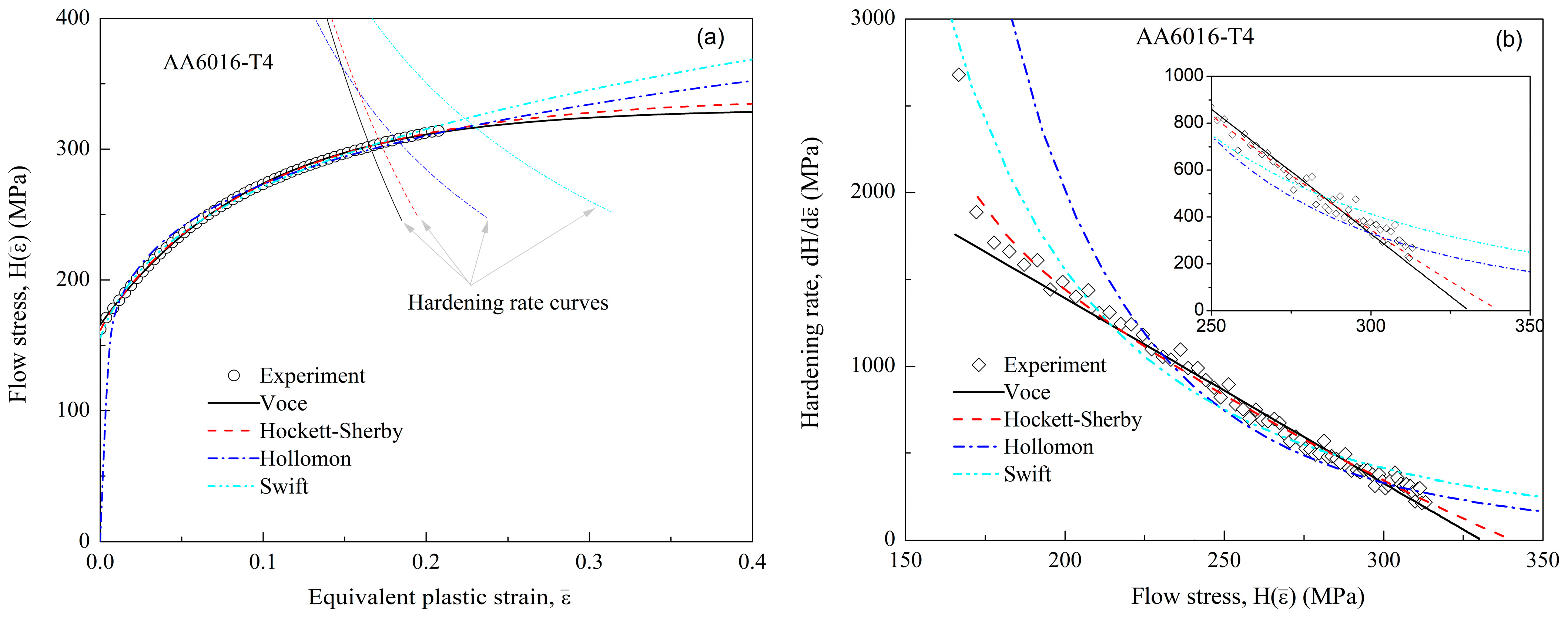
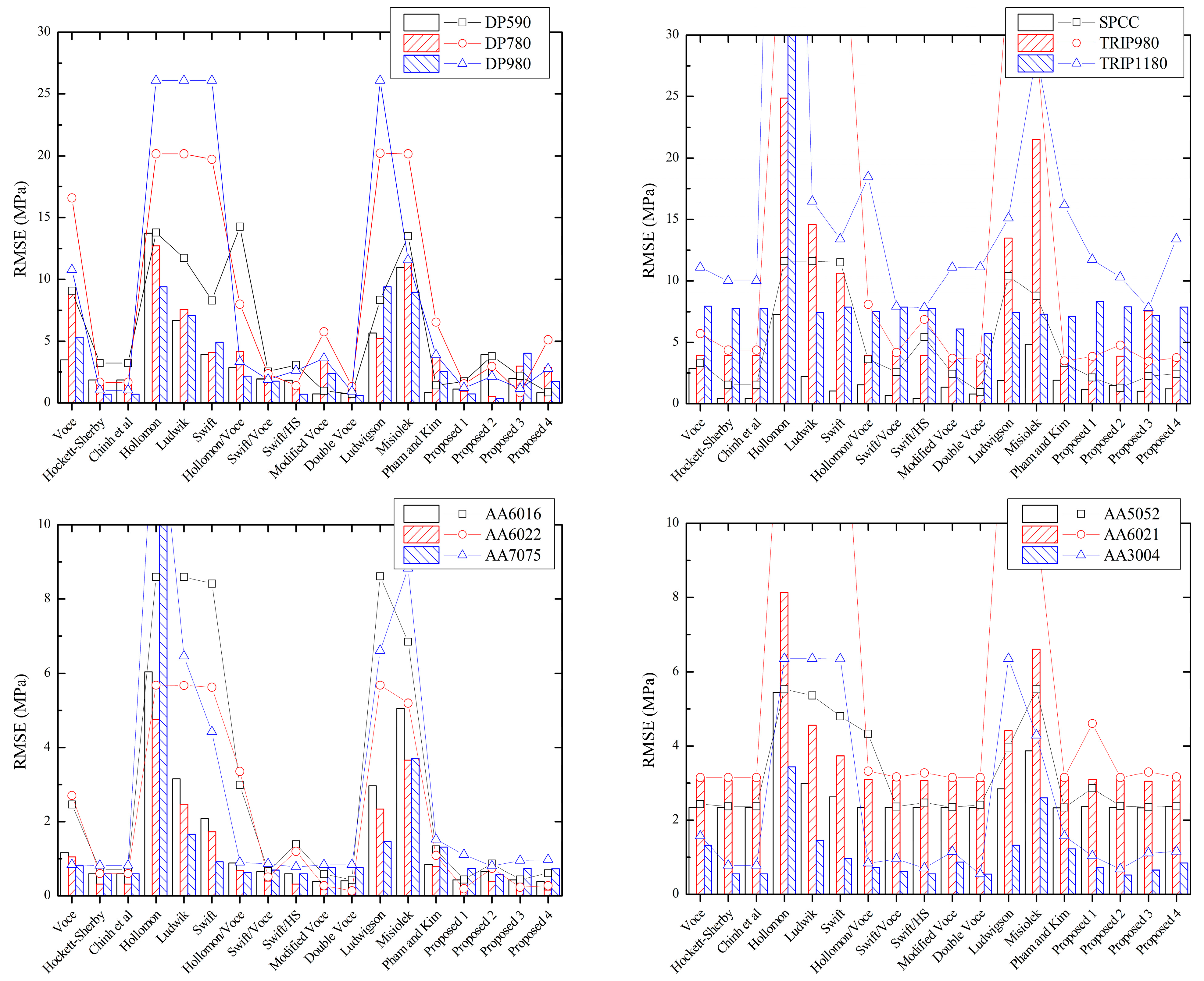
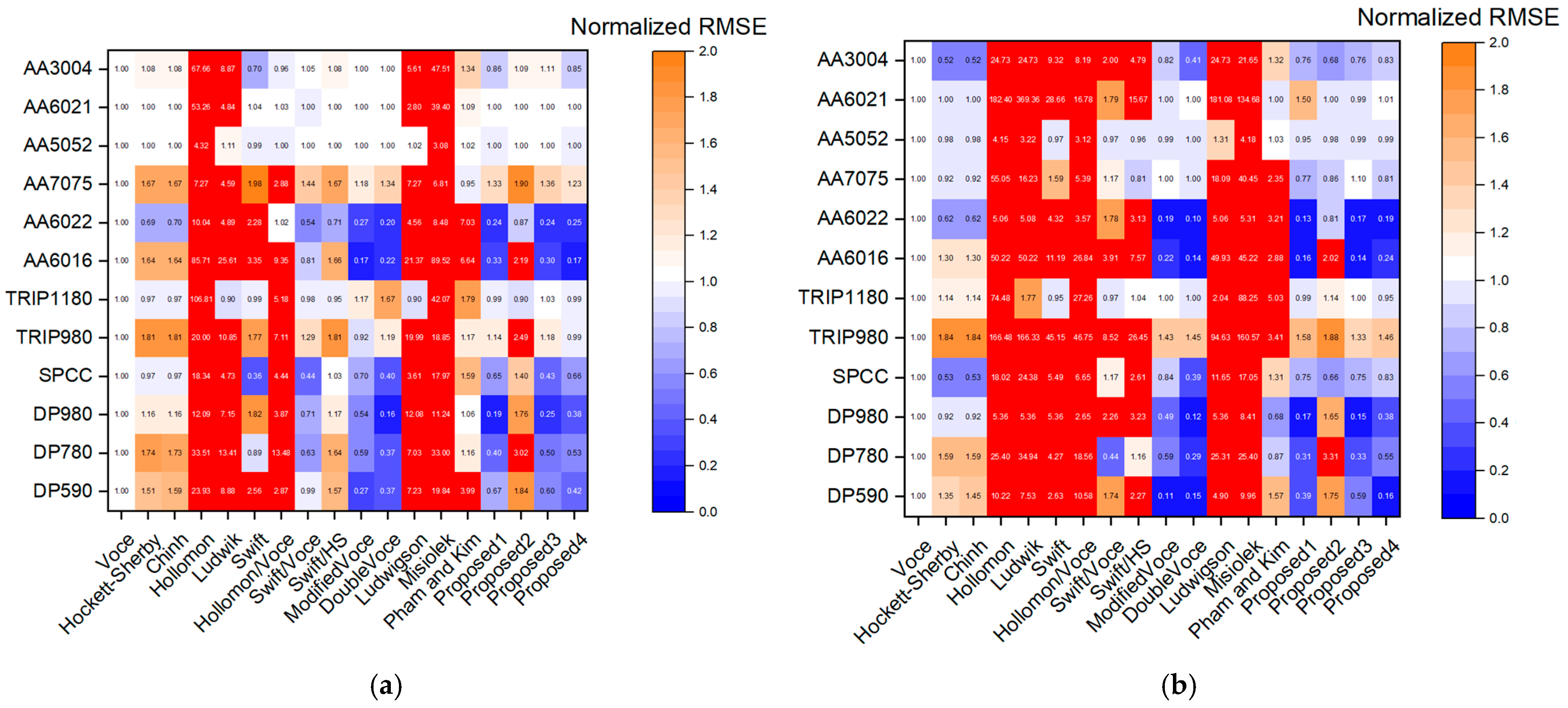
4.3. Calibration Result

The identified parameters of all hardening laws for 12 examined materials are reported in Tables S1–S12 in Supplementary Material. Figure 5 shows RMSE of the identified hardening laws for all tested materials. According to these figures, it is seen that there does not exist a hardening law that exhibits the best performance against the others. For a particular material in these figures, several hardening laws show good fitting results based on RMSE. For instance, the Hockett–Sherby and several combined hardening laws provide excellent RMSE for most of the tested materials. In this regard, all proposed hardening laws yield good RMSE of tested materials (RMSEs) that are more or less comparable to those of the mentioned hardening laws.

Furthermore, imposing a constraint on the fitting procedure always increases the RMSE, regardless of the used hardening formulation. In particular, the act significantly increases the RMSE of some specific hardening laws, such as the Hollomon, Ludwigson, and Misiolek models for many examined materials. In contrast, the RMSEs of several hardening laws, such as the Hockett–Sherby, combined Swift/Hockett–Sherby, and modified Voce models barely increase when the constrained curve fitting method is used. The comparison demonstrates the flexibility of these hardening laws and confirms their usefulness in practice, which has been proven in previous studies [15,45,46]. In addition, the proposed hardening laws appear to have enough flexibility for reproducing the flow curves of all investigated materials. Future studies should be conducted to address the potential of the proposed hardening laws in capturing the hardening behaviors of other materials.

4.4. Discussion

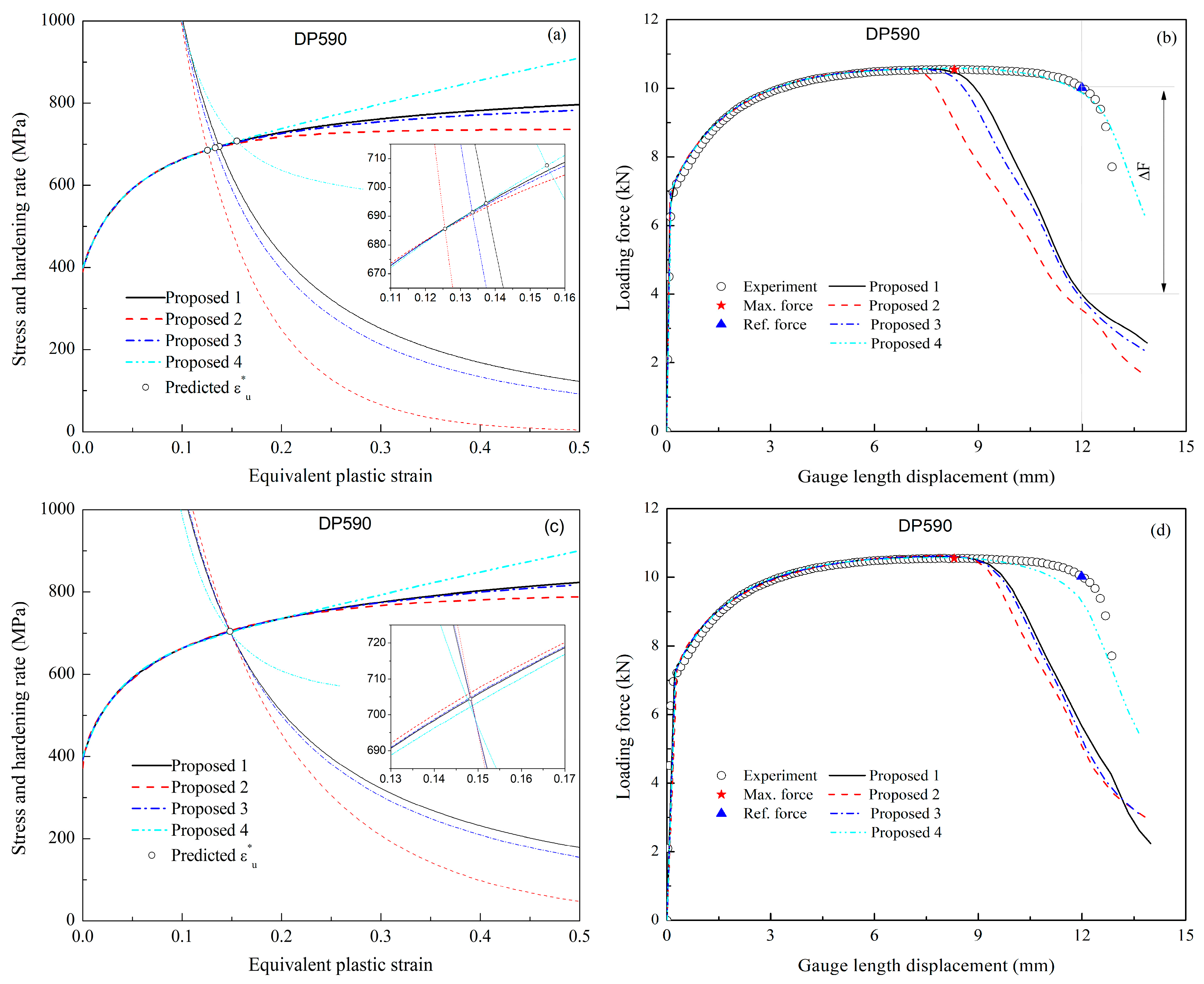
4.4.1. Diffuse Neck Prediction

As discussed before, the predictability of a hardening law for the diffuse neck indicated by the maximum homogeneous plastic strain, ${\epsilon }_u^{*}$ regards its accuracy in predicting the FLC of the tested material. Therefore, the difference between the experimental ${\epsilon }_u^{*}$ and a predicted value ${\tilde{\epsilon }}_u^{*}$ given by a hardening law is calculated as follows:

$${\delta }_1=\frac{{\tilde{\epsilon }}_u^{*}-{\epsilon }_u^{*}}{{\epsilon }_u^{*}}\times 100\%$$

(21)

Figure 6 presents the calculated ${\delta }_1$ based on the hardening laws identified by the common curve fitting method. As shown in this figure, the saturation laws frequently underestimated the diffuse neck of the tested material, indicated by negative values of ${\delta }_1$. Whereas, the power laws overestimated the phenomenon with positive values of ${\delta }_1$. In general, combined models (except for Ludwigson’s and Misiolek’s) provide better predictions. Compared to these combined models, the proposed hardening laws provide comparable predictions for ${\epsilon }_u^{*}$ of the investigated materials. It is noted that the proposed hardening laws take fewer parameters than these combined models.

4.4.2. Hardening Rate Curve Prediction

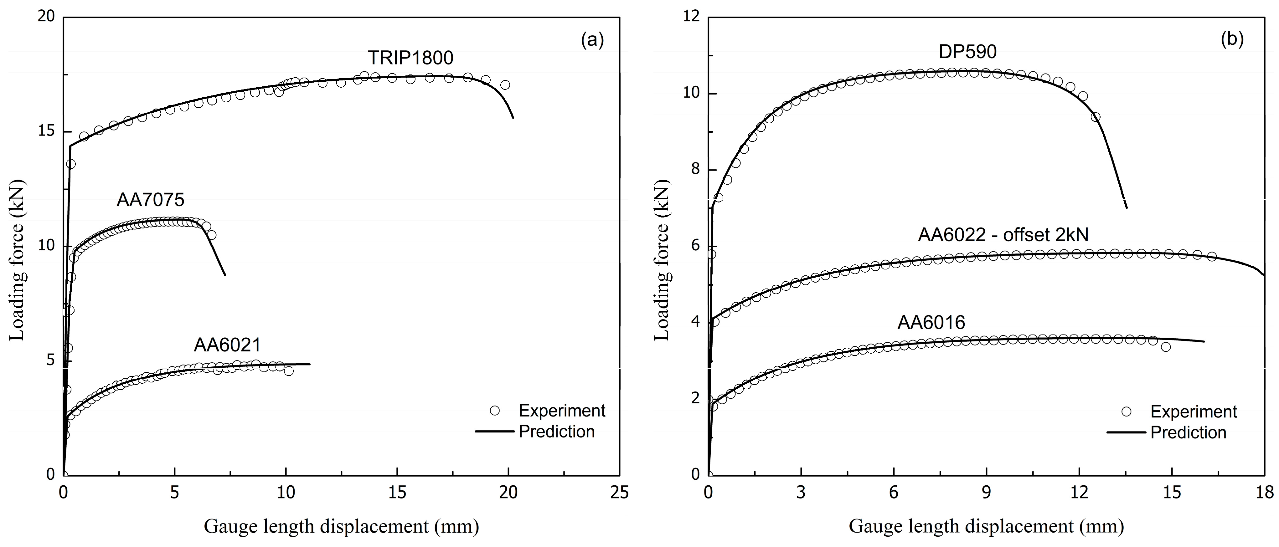
Following previous studies [47,48,49], a reference hardening rate curve is constructed for each material using five-order polynomials. These functions are the derivative of polynomials fitted to the experimental stress-strain data of the investigated materials. The difference between the reference hardening rate curve and the one of a hardening law is calculated by RMSE of evenly distributed 100 points between zero and ${\epsilon }_u^{*}$ of each curve. For each investigated material, the calculated RMSEs are normalized to the one of the Voce model and reported in Figure 7. In this figure, blue areas indicate better predictions, while red areas show predictions twice as bad as that of the Voce model.

It is seen from Figure 7 that several combined hardening laws, such as Swift/Hockett–Sherby, modified Voce, and double Voce models, derived good predictions for the hardening rate curves, no matter the constrained or unconstrained fitting method is used. The results of Proposed 1, 3, and 4 functions are promising, in that they are comparable to those of the before-mentioned models. The results presented in Figure 5, Figure 6 and Figure 7 demonstrate the potential of all proposed hardening laws in reproducing the experimental stress-strain data obtained from the UT test for the examined materials. Hence, their applications in numerical simulations of a forming process are deserving of further investigation.

5. Validation

This section deals with numerical validation for the identified hardening laws. These functions are employed to simulate UT tests of the investigated materials. Then, the simulated and measured tensile forces are compared to validate the accuracy of the imposed hardening laws in large strain ranges.

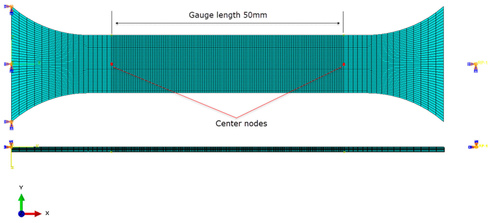
5.1. Finite Element Model

Several finite element (FE) models are developed in Abaqus/Standard package to simulate the UT tests. In these models, the first-order solid elements with reduced integration (C3D8R) are employed to model the testing coupon. Mesh size strongly influences the predicted tensile forces, especially after the maximum. The effect of mesh size on the simulation results of the UT tests for aluminum and steel alloys has been extensively investigated in [30,50,51]. Their studies recommended using a fine mesh on the gauge length region, in which the smallest edge size is in a range of [0.2; 0.3] mm to achieve convergence in simulated forces. Following the commendation, a fine mesh with the element size of 0.3 × 0.4 mm is designed in the center region. Since the thickness of the examined material is quite different, each FE model consists of five layers through the thickness direction to make sure that the corresponding element size is not more than 0.4 mm. Figure 8 shows the mesh on the specimen.

It is well-known that the numerical prediction of UT forces is insensitive to the material anisotropies, even though they are strongly affected the strain evolution of the deformed specimens [52]. Therefore, the von Mises yield function is adopted for plasticity modeling in these simulations because the tensile force predictions are used to evaluate simulation results.

During simulations, the left end section is fixed while a constant velocity is applied to the right one to deform the specimen. Reaction forces are recorded during simulation to report the tensile force predictions, while the gauge length displacements are calculated from the displacements of two center nodes, as shown in Figure 8. A Python code is developed to compare the experimental and simulated force-displacement curves.

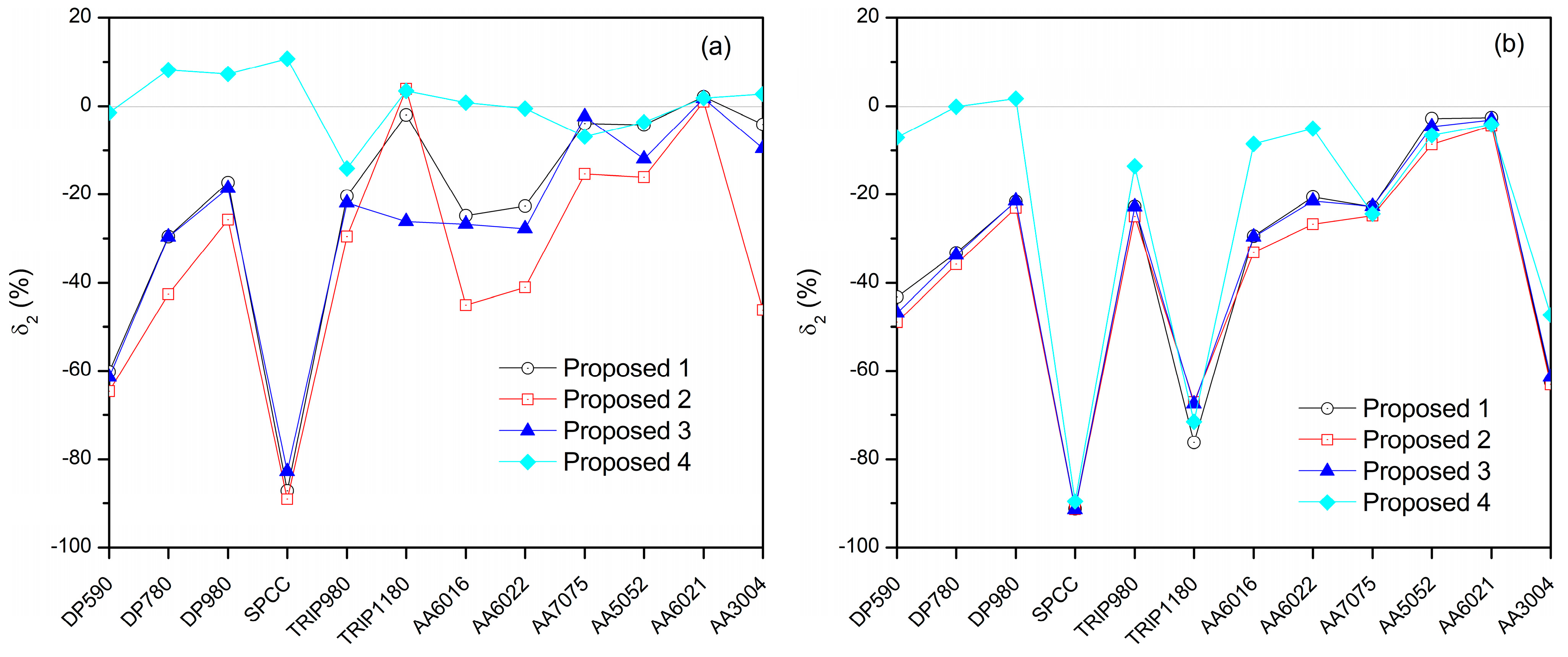
5.2. Effect of Calibration Method

Figure 9 shows comparisons between several hardening laws identified by the common and constrained curve fitting methods and their predictions for the UT forces of DP590 sheets. In addition, Figure 9a,c depict the predicted ${\epsilon }_u^{*}$ based on each hardening law, which indicates the onset of the diffuse neck estimated by the corresponding model. According to Figure 9a, the prediction of ${\tilde{\epsilon }}_u^{*}$ is strongly related to the post-necking estimation of a hardening law. The higher ${\tilde{\epsilon }}_u^{*}$ is predicted, the higher post-necking tensile force curve is derived. It is worth mentioning that all of these hardening laws approximated well the experimental stress-strain data obtained from the UT tests, as shown in Figure 5. Therefore, additional information should be considered to evaluate the usefulness of their prediction for the post-necking behavior of the tested material, which will be discussed in the next subsection.

Moreover, enforcing a constraint of ${\tilde{\epsilon }}_u^{*}$ in the fitting procedure results in the same prediction for the initiation of diffuse neck of different hardening laws, as shown in Figure 9c. However, adopting these hardening laws in UT simulations exposes underestimations for the tensile force curve after the maximum, as shown in Figure 9d. The drawback is believed to be caused by the uncertainty of ${\epsilon }_u^{*}$ determined from the experimental data. According to Figure 3a and Figure 4a, engineering stress-strain curves of many materials exhibit a wide range of strain in which a nearly unchanged tensile strength is observed. For such material, it is difficult to determine the initiation of the diffuse neck, as well as the corresponding value of ${\epsilon }_u^{*}$. Therefore, the constrained curve fitting method should be used with care, especially in determining the constraints.

5.3. Selection of a Proper Hardening Law

It is seen that numerical predictions for the tensile forces could agree well with the experimental data until the force maximum. However, force predictions in the post-necking ranges of different hardening models deviated largely from each other. It is well-established that the force predictions are sensitive to not only material modeling (i.e., material anisotropies and hardening law’s extrapolation to large strain ranges) but also numerical parameters (i.e., element type and mesh size). A primary study has been made to reduce the effects of numerical parameters in the developed FE models. Moreover, the effects of material anisotropies on the simulated forces are frequently ignored for many steel and aluminum alloy sheets [14,25,53]. Thus, the difference in predicted and measured tensile forces can be used to evaluate the quality of the hardening law’s extrapolation in the post-necking ranges. For this purpose, the force difference is estimated at a reference gauge length displacement by the following equation:

$${\delta }_2=\frac{F_r^{sim}-F_r^{exp}}{F_r^{exp}}\times 100\%$$

(22)

where $F_r^{sim}$ and $F_r^{exp}$ denote the simulated and experimental reference forces. It is noted that the reference force is related to the reference point of the engineering stress-strain curves shown in Figure 3a and Figure 4a for the investigated materials. Choosing different reference force points may affect insignificantly the calculated ${\delta }_2$ [41] and does not change the conclusions of this study.

Figure 10 shows the calculated δ₂ of the proposed hardening laws for all tested materials. According to Figure 10a, using the common curve fitting method yields a significant variation in calculated δ₂ based on different hardening laws. Adopting the constrained curve fitting method reduces the variation where the δ₂ calculations of these hardening laws are closer together. However, the constraints lead to underestimations for the tensile force of many materials. Therefore, it is suggested that the constrained method is applicable for limited materials.

For some materials such as TRIP1180, AA7075, and AA6021 sheets, several proposed models give good evaluations of δ₂. However, there exist several materials of which all of these hardening laws give unsatisfied δ₂ calculation, for instance, DP780, SPCC, and TRIP980 sheets. For such kinds of materials, a different hardening law or a different calibration method should be adopted to identify the parameters of the hardening laws. Hence, the calculated δ₂ of all mentioned hardening laws for all tested materials are reported in Supplementary Material (Figure S1). From this perspective, if there are a lot of hardening laws available for a particular investigated material, which one is adaptable will need to be determined.

Calibration of hardening law’s parameters is an optimization process, where the solution is a local minimum. Therefore, using different calibration methods perhaps derive different calibrated parameters. In addition to selecting a proper hardening law, a suitable calibration method should be considered carefully to determine parameters. The chosen one aims at achieving a balanced accuracy of the pre- and post-necking predictions of the identified hardening law. Hence, evaluating both the RMSE and δ₂ criteria could be considered to meet the demand. A small value of RMSE can be used as a necessary condition to ensure the accuracy of the selected hardening law in the pre-necking ranges. Whereas, the δ₂ can be used as a sufficient condition to qualify the goodness of the model’s predictions in the post-necking ranges. For example, the Proposed 1 provides good descriptions for several materials, such as TRIP1180, AA7075, and AA6021 sheets. In another hand, the Proposed 4 gives excellent results for DP590, AA6016, and AA6022 sheets. Figure 11 depicts their predictions of tensile forces for the mentioned materials. For other materials, one may choose a proper hardening law based on the results reported in Figure 5 and Figure S1.

6. Conclusions

This study discussed the formulation of common hardening laws in the literature, which are mainly used to describe the stress-strain relationships of automotive sheet metals. Experimental data show that the evolution of hardening rate according to the increment of the flow stress appears to be highly nonlinear. The use of either a saturation law or a power law seems to be sufficient for capturing the experimental stress-strain data obtained from the UT tests of the investigated materials. However, their extrapolation to large strain ranges may be unsatisfied, as demonstrated by their predictions for the diffuse neck and the hardening rate curves. Compared to these single functions, the combined hardening laws provide better predictions for the post-necking ranges. However, the number of parameters involved in these combinations are more than those of a single one. Increasing the number of parameters may cost more in the calibration process, especially if an advanced method, for example, the inverse finite element method, is applied.

Formulations of common hardening laws existing in the literature for sheet metals were discussed using their ODE. Based on these discussions, four phenomenological hardening laws for automotive sheet metals were presented, which requires four parameters in each model. Two saturation laws are similar to those presented in previous studies [6,42] but their formulas were constructed in different ways. Two power laws were newly proposed, according to the authors’ knowledge. The proposed hardening laws, in addition to the 14 hardening laws that exist in the literature, were tested for 12 sheet metals, including six steel and six aluminum alloy sheets. The common and constrained curve fitting methods were adopted to identify their parameters using experimental stress-strain data obtained from the UT tests. Applications of the proposed hardening laws in fitting to the flow stresses and predicting the diffuse neck, as well as the hardening rate curve of the tested materials, are comparable to those of several combined hardening laws. Within four involved parameters, the proposed functions may gain an advantage over the combined models if they are calibrated by an advanced method such as the inverse finite element method.

Applications of both common and constrained curve fitting methods for identifying hardening law’s parameters expose limitations. Additional information is needed to judge the goodness of the hardening laws identified by the common curve fitting method because their extrapolations to larger strain ranges are highly sensitive to the formulations of the imposed law. The constrained method should be used with care in determining a value of the maximum uniform plastic strain. Application of this method is only acceptable for limited materials examined in this study. From this perspective, the δ₂ criterion expressed in Equation (22) can be used as an indicator for choosing a proper hardening law of which the parameters were identified by curve fitting methods.

References

1. Trzepieciński, T. Recent developments and trends in sheet metal forming. Metals 2020, 10, 779. [Google Scholar] [CrossRef]
2. Gronostajski, Z.; Pater, Z.; Madej, L.; Gontarz, A.; Lisiecki, L.; Łukaszek-Sołek, A.; Łuksza, J.; Mróz, S.; Muskalski, Z.; Muzykiewicz, W.; et al. Recent development trends in metal forming. Arch. Civ. Mech. Eng. 2019, 19, 898–941. [Google Scholar] [CrossRef]
3. Ablat, M.A.; Qattawi, A. Numerical simulation of sheet metal forming: A review. Int. J. Adv. Manuf. Technol. 2017, 89, 1235–1250. [Google Scholar] [CrossRef]
4. Barlat, F.; Gracio, J.J.; Lee, M.G.; Rauch, E.F.; Vincze, G. An alternative to kinematic hardening in classical plasticity. Int. J. Plast. 2011, 27, 1309–1327. [Google Scholar] [CrossRef]
5. Banabic, D.; Carleer, B.; Comsa, D.S.; Kam, E.; Krasovskyy, A.; Mattiasson, K.; Sester, M.; Sigvant, M.; Zhang, X. Sheet Metal Forming Processes: Constitutive Modelling and Numerical Simulation; Springer: New York, NY, USA, 2010; ISBN 9783540881124. [Google Scholar]
6. Gronostajski, Z. The constitutive equations for FEM analysis. J. Mater. Process. Technol. 2000, 106, 40–44. [Google Scholar] [CrossRef]
7. Voce, E. The relationship between stress and strain for homogeneous deformation. J. Inst. Met. 1948, 74, 537–562. [Google Scholar]
8. Hockett, J.E.; Sherby, O.D. Large strain deformation of polycrystalline metals at low homologous temperatures. J. Mech. Phys. Solids 1975, 23, 87–98. [Google Scholar] [CrossRef]
9. Hollomon, J.H. Tensile deformation. Trans. AIME 1945, 162, 268–290. [Google Scholar]
10. Swift, H.W. Plastic instability under plane stress. J. Mech. Phys. Solids 1952, 1, 1–18. [Google Scholar] [CrossRef]
11. Pham, Q.T.; Lee, B.H.; Park, K.C.; Kim, Y.S. Influence of the post-necking prediction of hardening law on the theoretical forming limit curve of aluminium sheets. Int. J. Mech. Sci. 2018, 140, 521–536. [Google Scholar] [CrossRef]
12. Yoshida, K.; Ishii, A.; Tadano, Y. Work-hardening behavior of polycrystalline aluminum alloy under multiaxial stress paths. Int. J. Plast. 2014, 53, 17–39. [Google Scholar] [CrossRef]
13. Butuc, M.C.; Barata, A.; Gracio, J.J.; Duarte, J.F. A more general model for forming limit diagrams prediction. J. Mater. Process. Technol. 2002, 126, 213–218. [Google Scholar] [CrossRef]
14. Kim, J.H.; Serpantié, A.; Barlat, F.; Pierron, F.; Lee, M.G. Characterization of the post-necking strain hardening behavior using the virtual fields method. Int. J. Solids Struct. 2013, 50, 3829–3842. [Google Scholar] [CrossRef] [Green Version]
15. Kocks, U.F.; Mecking, H. Physics and phenomenology of strain hardening: The FCC case. Prog. Mater. Sci. 2003, 48, 171–273. [Google Scholar] [CrossRef]
16. Altan, T.; Tekkaya, A.E. Sheet Metal Forming: Fundamentals; ASM International: Russell, OH, USA, 2012; ISBN 1615038426. [Google Scholar]
17. Duflou, J.R.; Habraken, A.M.; Cao, J.; Malhotra, R.; Bambach, M.; Adams, D.; Vanhove, H.; Mohammadi, A.; Jeswiet, J. Single point incremental forming: State-of-the-art and prospects. Int. J. Mater. Form. 2018, 11, 743–773. [Google Scholar] [CrossRef]
18. Tekkaya, A.E. State-of-the-art of simulation of sheet metal forming. J. Mater. Process. Technol. 2000, 103, 14–22. [Google Scholar] [CrossRef]
19. Gothivarekar, S.; Coppieters, S.; Talemi, R.; Debruyne, D. Effect of bending process on the fatigue behaviour of high strength steel. J. Constr. Steel Res. 2021, 182, 106662. [Google Scholar] [CrossRef]
20. Eller, T.K.; Greve, L.; Andres, M.; Medricky, M.; Meinders, V.T.; Van Den Boogaard, A.H. Determination of strain hardening parameters of tailor hardened boron steel up to high strains using inverse FEM optimization and strain field matching. J. Mater. Process. Technol. 2016, 228, 43–58. [Google Scholar] [CrossRef]
21. Chinh, N.Q.; Horváth, G.; Horita, Z.; Langdon, T.G. A new constitutive relationship for the homogeneous deformation of metals over a wide range of strain. Acta Mater. 2004, 52, 3555–3563. [Google Scholar] [CrossRef]
22. Ludwik, P. Elemente der Technologischen Mechanik; Springer: Berlin/Heidelberg, Germany, 1909. [Google Scholar]
23. Saboori, M.; Champliaud, H.; Gholipour, J.; Gakwaya, A.; Savoie, J.; Wanjara, P. Extension of flow stress–strain curves of aerospace alloys after necking. Int. J. Adv. Manuf. Technol. 2016, 83, 313–323. [Google Scholar] [CrossRef]
24. Park, S.J.; Lee, K.; Cerik, B.C.; Choung, J. Ductile fracture prediction of EH36 grade steel based on Hosford–Coulomb model. Ships Offshore Struct. 2019, 14, 219–230. [Google Scholar] [CrossRef]
25. Coppieters, S.; Cooreman, S.; Sol, H.; Van Houtte, P.; Debruyne, D. Identification of the post-necking hardening behaviour of sheet metal by comparison of the internal and external work in the necking zone. J. Mater. Process. Technol. 2011, 211, 545–552. [Google Scholar] [CrossRef]
26. Sung, J.H.; Kim, J.H.; Wagoner, R.H. A plastic constitutive equation incorporating strain, strain-rate, and temperature. Int. J. Plast. 2010, 26, 1746–1771. [Google Scholar] [CrossRef]
27. Ha, J.; Baral, M.; Korkolis, Y.P. Plastic anisotropy and ductile fracture of bake-hardened AA6013 aluminum sheet. Int. J. Solids Struct. 2018, 155, 123–139. [Google Scholar] [CrossRef]
28. Capilla, G.; Hamasaki, H.; Yoshida, F. Determination of uniaxial large-strain workhardening of high-strength steel sheets from in-plane stretch-bending testing. J. Mater. Process. Technol. 2017, 243, 152–169. [Google Scholar] [CrossRef]
29. Ben-Elechi, S.; Khelifa, M.; Bahloul, R. Sensitivity of friction coefficients, material constitutive laws and yield functions on the accuracy of springback prediction for an automotive part. Int. J. Mater. Form. 2021, 14, 323–340. [Google Scholar] [CrossRef]
30. Zhao, K.; Wang, L.; Chang, Y.; Yan, J. Identification of post-necking stress-strain curve for sheet metals by inverse method. Mech. Mater. 2016, 92, 107–118. [Google Scholar] [CrossRef]
31. Min, J.; Stoughton, T.B.; Carsley, J.E.; Lin, J. Compensation for process-dependent effects in the determination of localized necking limits. Int. J. Mech. Sci. 2016, 117, 115–134. [Google Scholar] [CrossRef] [Green Version]
32. Koc, P.; Štok, B. Computer-aided identification of the yield curve of a sheet metal after onset of necking. Comput. Mater. Sci. 2004, 31, 155–168. [Google Scholar] [CrossRef]
33. Ludwigson, D.C. Modified stress-strain relation for FCC metals and alloys. Metall. Trans. 1971, 2, 2825–2828. [Google Scholar] [CrossRef]
34. Samuel, K.G.; Rodriguez, P. On power-law type relationships and the Ludwigson explanation for the stress-strain behaviour of AISI 316 stainless steel. J. Mater. Sci. 2005, 40, 5727–5731. [Google Scholar] [CrossRef]
35. Lavakumar, A.; Sarangi, S.S.; Chilla, V.; Narsimhachary, D.; Ray, R.K. A “new” empirical equation to describe the strain hardening behavior of steels and other metallic materials. Mater. Sci. Eng. A 2021, 802, 140641. [Google Scholar] [CrossRef]
36. Wang, N.; Ilinich, A.; Chen, M.; Luckey, G.; D’Amours, G. A comparison study on forming limit prediction methods for hot stamping of 7075 aluminum sheet. Int. J. Mech. Sci. 2019, 151, 444–460. [Google Scholar] [CrossRef]
37. Fan, R.; Chen, M.; Wu, Y.; Xie, L. Prediction and experiment of fracture behavior in hot press forming of a TA32 titanium alloy rolled sheet. Metals 2018, 8, 985. [Google Scholar] [CrossRef] [Green Version]
38. Pham, Q.T.; Kim, Y.S. Identification of the plastic deformation characteristics of AL5052-O sheet based on the non-associated flow rule. Met. Mater. Int. 2017, 23, 254–263. [Google Scholar] [CrossRef]
39. Pham, Q.T.; Oh, S.H.; Kim, Y.S. An efficient method to estimate the post-necking behavior of sheet metals. Int. J. Adv. Manuf. Technol. 2018, 98, 2563–2578. [Google Scholar] [CrossRef]
40. Pham, Q.T.; Lee, M.G.; Kim, Y.S. New procedure for determining the strain hardening behavior of sheet metals at large strains using the curve fitting method. Mech. Mater. 2021, 154, 103729. [Google Scholar] [CrossRef]
41. Pham, Q.T.; Nguyen-Thoi, T.; Ha, J.; Kim, Y.-S. A Hybrid Fitting-Numerical Method for Determining Strain Hardening Behavior of Sheet Metals. Mech. Mater. 2021, 161, 104031. [Google Scholar] [CrossRef]
42. Sahoo, S.K.; Dhinwal, S.S.; Vu, V.Q.; Toth, L.S. A new macroscopic strain hardening function based on microscale crystal plasticity and its application in polycrystal modeling. Mater. Sci. Eng. A 2021, 823, 141634. [Google Scholar] [CrossRef]
43. Nguyen, N.T.; Seo, O.S.; Lee, C.A.; Lee, M.G.; Kim, J.H.; Kim, H.Y. Mechanical behavior of AZ31B Mg alloy sheets under monotonic and cyclic loadings at room and moderately elevated temperatures. Materials 2014, 7, 1271–1295. [Google Scholar] [CrossRef] [Green Version]
44. Noder, J.; Butcher, C. A comparative investigation into the influence of the constitutive model on the prediction of in-plane formability for Nakazima and Marciniak tests. Int. J. Mech. Sci. 2019, 163, 105138. [Google Scholar] [CrossRef]
45. Nes, E. Modelling of work hardening and stress saturation in FCC metals. Prog. Mater. Sci. 1997, 41, 129–193. [Google Scholar] [CrossRef]
46. Salvado, F.C.; Teixeira-Dias, F.; Walley, S.M.; Lea, L.J.; Cardoso, J.B. A review on the strain rate dependency of the dynamic viscoplastic response of FCC metals. Prog. Mater. Sci. 2017, 88, 186–231. [Google Scholar] [CrossRef] [Green Version]
47. Chen, F.; Cui, Z.; Chen, S. Recrystallization of 30Cr2Ni4MoV ultra-super-critical rotor steel during hot deformation. Part I: Dynamic recrystallization. Mater. Sci. Eng. A 2011, 528, 5073–5080. [Google Scholar] [CrossRef]
48. Nabizada, A.; Zarei-Hanzaki, A.; Abedi, H.R.; Barati, M.H.; Asghari-Rad, P.; Kim, H.S. The high temperature mechanical properties and the correlated microstructure/texture evolutions of a TWIP high entropy alloy. Mater. Sci. Eng. A 2021, 802, 140600. [Google Scholar] [CrossRef]
49. Shi, P.; Zhong, Y.; Li, Y.; Ren, W.; Zheng, T.; Shen, Z.; Yang, B.; Peng, J.; Hu, P.; Zhang, Y.; et al. Multistage work hardening assisted by multi-type twinning in ultrafine-grained heterostructural eutectic high-entropy alloys. Mater. Today 2020, 41, 62–71. [Google Scholar] [CrossRef]
50. Mu, Z.; Zhao, J.; Yua, G.; Huang, X.; Meng, Q.; Zhai, R. Hardening model of anisotropic sheet metal during the diffuse instability necking stage of uniaxial tension. Thin-Walled Struct. 2021, 159, 107198. [Google Scholar] [CrossRef]
51. Maček, A.; Starman, B.; Mole, N.; Halilovič, M. Calibration of Advanced Yield Criteria Using Uniaxial and Heterogeneous Tensile Test Data. Metals 2020, 10, 542. [Google Scholar] [CrossRef]
52. Lou, Y.; Huh, H. Prediction of ductile fracture for advanced high strength steel with a new criterion: Experiments and simulation. J. Mater. Process. Technol. 2013, 213, 1284–1302. [Google Scholar] [CrossRef]
53. Tao, H.; Zhang, N.; Tong, W. An iterative procedure for determining effective stress-strain curves of sheet metals. Int. J. Mech. Mater. Des. 2009, 5, 13–27. [Google Scholar] [CrossRef]
Figure 1. Applications of four hardening laws in capturing the experimental data obtained from the uniaxial tensile test of AA6016-T4 sheets. Experimental data after [11]. (a) Stress-strain curves. (b) Hardening rate—flow stress curves.
Metals 12 00578 g001
Figure 2. Application of a linear combined Swift and Voce models for AA6016-T4 sheets. Experimental data after [11].
Metals 12 00578 g002
Figure 3. Stress-strain data obtained from uniaxial tensile tests for six steel sheets. (a) Engineering stress-strain curves. (b) True stress-strain curves.
Metals 12 00578 g003
Figure 4. Stress-strain data obtained from uniaxial tensile tests for six aluminum alloy sheets. (a) Engineering stress-strain curves. (b) True stress-strain curves.
Metals 12 00578 g004
Figure 5. RMSE of the identified hardening laws for tested materials. Column charts indicate the results of the common curve fitting method; opened symbols indicate the results of the constrained curve fitting method.
Metals 12 00578 g005
Figure 6. Percentage errors of diffuse neck prediction of all examined hardening laws identified by the common curve fitting method.
Metals 12 00578 g006
Figure 7. Normalized RMSE of hardening rate predictions. (a) Hardening laws identified by the common curve fitting method. (b) Hardening laws identified by the constrained curve fitting method.
Metals 12 00578 g007
Figure 8. Mesh on the specimen.
Metals 12 00578 g008
Figure 9. Comparison between the experimental and predicted tensile forces according to gauge length displacement of DP590 sheets. (a) Hardening laws identified by the common curve fitting method. (b) Tensile force predictions of the hardening laws reported in (a). (c) Hardening laws identified by the constrained curve fitting method. (d) Tensile force predictions of the hardening laws reported in (c).
Metals 12 00578 g009
Figure 10. Calculated δ2 of the identified hardening laws for tested materials. (a) Hardening laws identified by the common curve fitting method. (b) Hardening laws identified by the constrained curve fitting method.
Metals 12 00578 g010
Figure 11. Tensile force predictions of (a) Proposed 1 and (b) Proposed 4 models for several materials.
Metals 12 00578 g011