Coupling Flotation Rate Constant and Viscosity Models

Abstract

In a flotation process, the particle–bubble and particle–particle interactions are key factors influencing collection efficiencies. In this work, the generalized Sutherland equation collision model and the modified Dobby–Finch attachment model for potential flow conditions were used to calculate the efficiencies of particle–bubble collision and attachment, respectively, for a flotation particle size of 80 μm. The negative effects of increase in the suspension viscosity due to the presence of fine particles on the flotation performance of fine particles have been reported, but there is no overarching model coupling the suspension viscosity and the flotation performance in the literature. Therefore, our study addressed this very important research gap and incorporated the viscosity model as a function of solid concentration, shear rate, and particle size into a flotation rate constant model that was proposed and conducted for the first time. This is quite a unique approach because the previously developed flotation rate constant model has never been coupled with a suspension rheology model taking into account the solid particle concentration and shear rate, although they are very important flotation variables in practice. The effect of the presence of ultra-fine/fine particles on the viscosity of the suspension and the flotation efficiencies and rate constant of flotation particle size of 80 μm were also investigated in order to better understand the mechanism of the problematic behavior of ultra-fine/fine particles in flotation. This coupling study started with the simplest case: flowing suspensions of inert, rigid, monomodal spherical particles (called hard spheres). Even for hard spheres, the effect of shear rate and particle size which produces deviation from the ideal case (constant viscosity at constant temperature regardless of shear rate) was clearly identified. It was found that the suspension viscosity increases with the decrease in fine/ultra-fine particle size (i.e., 1 µm–8 nm) and at higher solid particle concentration. Then, the colloidal particle suspensions, where interparticle forces play a significant role, were also studied. The suspension viscosity calculated for both cases was incorporated into the flotation efficiencies and rate constant models and discussed in terms of the effects of the presence of ultra-fine and fine particles on the flotation kinetics of flotation particle size of 80 μm.

1. Introduction

Mechanical froth flotation is one of the most widely used processes for separating valuable minerals in mineral processing plants. It also has extensive applications in different industries such as paper [1], plastic [2], petrochemical [3], and waste recycling [4]. Flotation takes place in three different phases (i.e., solid (particles), liquid (water), and gas (bubbles)).

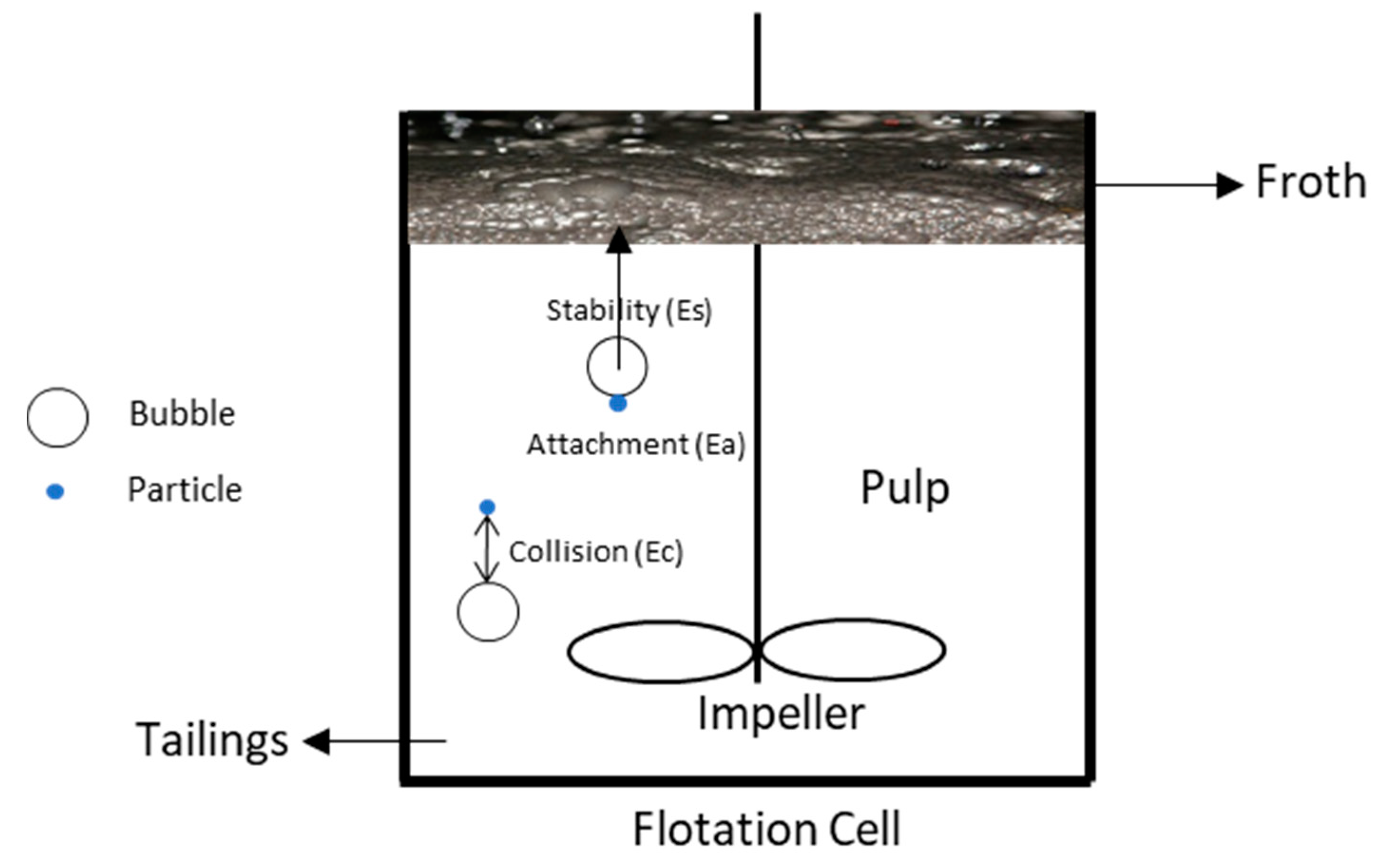
Bubble–particle interactions are widely acknowledged to be the most important sub-process in froth flotation. These interactions can be quantified based on statistical approaches on successful transfer of particles on bubbles towards the froth phase and then concentrates. These interactions were categorized into collision ($E_{\mathrm{c}}$), attachment ($E_{\mathrm{a}}$), and stability ($E_{\mathrm{s}}$) sub-processes [5]. A clear understanding of these sub-processes is basically essential in the estimation of flotation kinetic rates. Figure 1 shows a schematic overview of the sub-processes $\left(E_{\mathrm{c}}\right)$, $\left(E_{\mathrm{a}}\right)$, and $\left(E_{\mathrm{s}}\right)$ involved in the overall process of froth flotation [6], and their details will be described in Section 2.

The mechanisms of particle–bubble interactions control flotation selectivity and collection efficiency [7]. Flotation selectivity is a measure of the relative recovery of the hydrophobic particles (referred to as valuable mineral(s) in direct flotation) to that of the hydrophilic particles (referred to as non-valuable mineral(s) or gangue) [8]. The collection efficiency is the probability that the colliding bubble and particle will form a permanent aggregate, resulting in a successful transfer of particle into the concentrate, referred to as orthokinetic heterocoagulation in flotation science [9,10].

To explain and quantify the contributions of collision $\left(E_{\mathrm{c}}\right)$, attachment $\left(E_{\mathrm{a}}\right)$, and stability $\left(E_{\mathrm{s}}\right)$ efficiencies in particle–bubble attachment, an analytical model has been developed and used under turbulent flotation conditions, referred to as a general flotation kinetic model, which allows us to calculate the flotation rate constant as a function of particle size with measurable particle, bubble, and hydrodynamic quantities [5,11]. The flotation rate is the rate of valuable material/particle recovery in a flotation product (concentrate) per unit time. Numerous researchers have studied the kinetics aspects of froth flotation, paying special attention to particle and bubble sizes and their complex interactions in flotation cells [12,13].

The suspension viscosity, which is affected by the presence of fine/ultra-fine particles as well as the clay minerals [6], also plays a key role in influencing the flotation rate constant. Several studies showed that the presence of fine particles increases the pulp viscosity and thus has a negative effect on the flotation kinetics [14,15,16,17,18,19,20]. The suspension viscosity is affected by the solid concentration, shear rate, and particle size [21,22]. However, to the best knowledge of the authors, there is no study which incorporates these parameters into the flotation rate constant model by coupling with a suspension viscosity model. This incorporation was performed in this study for the first time.

A number of studies have indicated a strong relationship between flotation performance and pulp rheological property [17,18,23,24,25]. A higher pulp viscosity usually corresponds to a lower recovery of valuable minerals. In the pulp zone of a flotation cell (Figure 1), a high pulp viscosity can result in increased turbulence damping, poor gas dispersion, a reduced mobility of particles and mineralized bubbles, and a low particle–bubble collision efficiency [26,27]. All of these factors can lead to a reduced flotation efficiency.

In operating flotation plants, the viscosity of the pulp can vary significantly. Zhang (2014) [23] reported a change in the pulp viscosity in a flotation cell between 0.001619 to 0.000641 Pa s while evaluating the effect of viscosity changes on bubble size in a mechanical flotation cell. Chen et al. (2017) [18] studied the effect of amorphous silica on pulp rheology and copper flotation and reported the apparent viscosity of 0.286 Pa s at 20 vol.% amorphous silica suspension, and 0.093 Pa s at 20 vol.% quartz suspension; both of these values were obtained at a shear rate of 100 s⁻¹.

Farrokhpay et al. (2011) [24] studied the processing of low-grade coarse composite particles in porphyry copper ores and used the viscosity of 0.0076 Pa s at 50 vol.% glycerol–water mixture. Farrokhpay et al. (2016) [25] studied the behavior of swelling clays vs. non-swelling clays in flotation, and they found out that copper recovery was decreased drastically (90% to 80%) in the presence of 15 wt.% swelling clay, montmorillonite; however, in the presence of 15 wt.% non-swelling clays, illite and kaolinite, the copper recovery decreased slightly to 87% and 88%, respectively. The copper grade decreased from 18% to about 1% in the presence of 30 wt.% and 15 wt.% of kaolinite and montmorillonite, respectively, and to about 5% in the presence of 30 wt.% illite. They reported that the apparent viscosities of the ore slurry in the presence of 15 wt.% montmorillonite, 30 wt.% of kaolinite, and 30 wt.% illite at a shear rate of 100 s⁻¹ were 0.17, 0.03, and 0.02 Pa s, respectively.

Farrokhpay et al. (2018) [17] studied the behavior of talc and mica in copper ore flotation and reported that the viscosities of the ore slurry in the presence of 7.5 wt.% talc and 30 wt.% muscovite at a shear rate of 100 s⁻¹ were 0.038 and 0.012 Pa s, respectively. Forbes et al. (2014) [28] studied the effect of rheology and slime coating on the natural floatability of chalcopyrite in a clay-rich flotation pulp and reported viscosity values between 0.001 and 0.15 Pa s. They reported copper recovery of 92% at quartz/kaolinite content of 100/0; however, with the change in quartz/kaolinite content (i.e., 70/30, and 30/70), the copper recovery was reduced to 87% and 82%, respectively. Table 1 summarizes the literature discussing the influence of the suspension viscosity on the flotation performance.

It has been demonstrated that there is a considerable variation of the shear rate distribution inside the flotation cell with the highest values close to the impeller [29]. The other areas in the flotation cell may have relatively small shear rate values, which can be even close to zero [20]. This causes the ore–clay mixtures, which are non-Newtonian, to have different shear stresses and viscosities at different locations in the flotation cell.

In our recent article [6], the correlation between flotation and rheology of fine particle suspensions was reviewed. The presence of values (e.g., critical raw materials) in fine/ultra-fine particles/grains in a complex manner has defined those ores as complex. There has been increasing demand for the beneficiation of complex ores, due to the noticeable decrease in the accessibility of high-grade and easily extractable ores. In order to maintain the sustainable use of limited resources, the effective beneficiation of complex ores is urgently required [30]. It can be successfully achieved only with selective particle/mineral dispersion/liberation and the assistance of mineralogical and fine particle characterization, including a proper understanding of the rheological behavior of complex ores in the context of fine particle separation/processing.

In this work, the parameters which affect the viscosity of flotation pulp (i.e., solid concentration, shear rate, and particle size) were studied in detail. Three cases of particles are discussed: (a) non-interacting non-Brownian hard spheres, (b) non-interacting Brownian hard spheres, and (c) interacting colloidal particles. Modified Krieger–Dougherty model and our predictive model developed for the viscosity of fine/ultra-fine particles were used to calculate the relative viscosity, and then the suspension viscosity. The particle–particle interactions (van der Waals and electric double-layer interactions) of colloidal particles were addressed by using the Derjaguin–Landau–Verwey–Overbeek (DLVO) theory [31,32]. The calculated suspension viscosity was then incorporated into the flotation kinetic model to calculate the flotation efficiencies and rate constant.

In this article, Section 2 will introduce the theoretical background for the modeling work performed in this study. Section 3 will introduce the results and discussion on the modeling work, followed by Section 4 with conclusions.

Table 1. Summary of the literature discussing the influence of change in viscosity on flotation performance.

Researcher	Reported Suspension Viscosity	Flotation Results (Rate Constant or Recovery/Grade)	References
Farrokhpay et al., 2011	The viscosity of 50 vol.% glycerol–water mixture, used in their study, was 0.0076 Pa s.	The recovery of coarse composite copper-bearing particles (+210 μm) of porphyry copper ore, recovered in the tailings of rougher, at a grind size of d80 = 250 μm, increased from 83 to 90% with the increase in viscosity from 0.001 to 0.0076 Pa s.	[24]
Shabalala et al., 2011	The viscosity of kaolin ore slurry increased exponentially to the maximum values of between 0.03 and 0.08 Pa s with the increase in solid concentration from 15 to 40 wt.% of kaolin.	Bubble size generated within kaolin ore suspension decreased from 1 to 0.65 mm with the increase in solid concentration from 30 to 40 wt.% at an impeller speed of 650 rpm.	[26]
Forbes et al., 2014	The viscosity of pulp containing chalcopyrite and clay minerals (kaolinite and quartz) was found between 0.001 and 0.15 Pa s.	The recovery of chalcopyrite (copper) was 92% at quartz/kaolinite content of 100/0; however, with the change in quartz/kaolinite ratio (i.e., 70/30 and 30/70), the chalcopyrite recovery reduced to 87% and 82%, respectively.	[28]
Cruz et al., 2015	The viscosity of copper–gold ore slurry increased from 0.0035 to 0.014 Pa s with the increase of solid concentration of bentonite from 0 to 15 wt.% at a shear rate of 100 s−1.	The baseline flotation of their ore (i.e., 100 wt.% ore without bentonite/kaolinite) resulted in a copper recovery of 92% at a grade of 10% copper, and 81% gold recovery at a grade of 7 ppm gold. The addition of 15 wt.% bentonite to the ore (100 wt.%) decreased the recovery (i.e., copper recovery from 92 to 83% and gold recovery from 81 to 64%) and slightly decreased in copper and gold grades from 10 to 8% and 7 ppm to 5 ppm, respectively. The addition of 30 wt.% kaolinite to the ore (100 wt.%) did not decrease copper and gold recoveries but did decrease copper and gold grades from 10 to 2% and 7 ppm to 1 ppm, respectively.	[20]
Wang et al., 2015	The apparent viscosity of Telfer clean ore increased from 0.001 to 0.008 Pa s with the increase in solid concentration of bentonite from 5 to 25 wt.% at a shear rate of 100 s−1.	The copper recovery decreased from 76 to 25% with the increase in solid concentration of bentonite from 0 to 20 wt.%; however, it slightly decreased the copper grade from 5.1 to 5%. The copper recovery decreased from 80 to 67% with the increase in solid concentration of kaolin from 0 to 20 wt.%; however, it decreased the copper grade from 5 to 4%.	[16]
Zhang & Peng, 2015	The apparent viscosity of a copper–gold ore increased from 0.0018 to 0.0076 Pa s with the increase in solid concentration of bentonite from 0 to 15 wt.% at a shear rate of 100 s−1.	The copper recovery decreased from 82 to 60% with the increase in solid concentration of bentonite from 0 to 15 wt.%. The gold recovery decreased from 78 to 65% with the increase in solid concentration of bentonite from 0 to 15%.	[14]
Farrokhpay et al., 2016	The apparent viscosity of their copper ore slurry in the presence of 15 wt.% montmorillonite, 30 wt.% of kaolinite, and 30 wt.% illite at a shear rate of 100 s−1 was 0.17, 0.03, and 0.02 Pa s, respectively.	The copper recovery decreased (90 to 80%) in the presence of 15 wt.% swelling clay (montmorillonite); however, in the presence of 15 wt.% non-swelling clays (illite and kaolinite), the copper recovery decreased slightly to 87% and 88%, respectively. The copper grade decreased from 18% to about 1% in the presence of both 30 wt.% of kaolinite and 15 wt.% of montmorillonite, respectively; however, it decreased to about 5% in the presence of 30% illite. The copper ore flotation rate constants were 0.51 s−1 and 0.49 s−1 in the presence of 15 wt.% of kaolinite and 15 wt.% of illite, respectively, and 0.33 s−1 in the presence 15 wt.% of montmorillonite, as compared with the copper ore flotation rate constant of 0.70 s−1 in the absence of clay minerals.	[25]
Basnayaka et al., 2017	The viscosity of gold ore increased from 0.0018 to 0.0035 Pa s by the addition of 10 wt.% kaolin at pH 7, a shear rate of 100 s−1, and polyacrylate depressant concentration of 0 and 200 g/t, respectively; however, by the addition of 5 wt.% bentonite, the viscosity increased to 0.0060 Pa s, under the same conditions.	The flotation rate constant of their gold-bearing pyrite ore was decreased from 13.71 to 3.37 s−1 (822.6 to 202.2 min−1) without and with the presence of 10 wt.% kaolin at pH 7, air rate of 5 L/min, and polyacrylate depressant concentration of 0 and 200 g/t, respectively. The presence of bentonite under same conditions reduced the flotation rate constant to 4.14 s−1 (248.4 min−1).	[33]
Chen et al., 2017	The apparent viscosity of amorphous silica and quartz suspension increased from 0.109 to 0.147 Pa s with the increase in the concentration of amorphous silica (in amorphous silica and quartz suspension) from 30 to 50 vol.%, at a shear rate of 100 s−1.	The copper recovery dropped sharply from 95 to 63.6% after the percentage of amorphous silica increased from 30 to 50 vol.%. The copper grade decreased slightly from 3.9 to 3.8% with the increase in the concentration of amorphous silica (in amorphous silica and quartz suspension) from 30 to 50 vol.%.	[18]
Farrokhpay et al., 2018	The viscosity of their copper ore slurry increased from 0.010 to 0.038 Pa s with the increase in solid concentration of muscovite from 0 to 30 wt.% at a shear rate of 100 s−1; however, with the increase in solid concentration of talc from 0 to 7.5 wt.%, there was a slight increase in the slurry viscosity from 0.010 to 0.012 Pa s, at a shear rate of 100 s−1.	The flotation grade decreased (19 to 2%) with the increase in solid concentration of muscovite from 0 to 30 wt.%; however, the change in the recovery was reported negligible. The flotation recovery (90 to 83%) and grade (19 to 2%) decreased with the increase in solid concentration of talc from 0 to 7.5 wt.%.	[17]

Table 1. Summary of the literature discussing the influence of change in viscosity on flotation performance.

Researcher	Reported Suspension Viscosity	Flotation Results (Rate Constant or Recovery/Grade)	References
Farrokhpay et al., 2011	The viscosity of 50 vol.% glycerol–water mixture, used in their study, was 0.0076 Pa s.	The recovery of coarse composite copper-bearing particles (+210 μm) of porphyry copper ore, recovered in the tailings of rougher, at a grind size of d80 = 250 μm, increased from 83 to 90% with the increase in viscosity from 0.001 to 0.0076 Pa s.	[24]
Shabalala et al., 2011	The viscosity of kaolin ore slurry increased exponentially to the maximum values of between 0.03 and 0.08 Pa s with the increase in solid concentration from 15 to 40 wt.% of kaolin.	Bubble size generated within kaolin ore suspension decreased from 1 to 0.65 mm with the increase in solid concentration from 30 to 40 wt.% at an impeller speed of 650 rpm.	[26]
Forbes et al., 2014	The viscosity of pulp containing chalcopyrite and clay minerals (kaolinite and quartz) was found between 0.001 and 0.15 Pa s.	The recovery of chalcopyrite (copper) was 92% at quartz/kaolinite content of 100/0; however, with the change in quartz/kaolinite ratio (i.e., 70/30 and 30/70), the chalcopyrite recovery reduced to 87% and 82%, respectively.	[28]
Cruz et al., 2015	The viscosity of copper–gold ore slurry increased from 0.0035 to 0.014 Pa s with the increase of solid concentration of bentonite from 0 to 15 wt.% at a shear rate of 100 s−1.	The baseline flotation of their ore (i.e., 100 wt.% ore without bentonite/kaolinite) resulted in a copper recovery of 92% at a grade of 10% copper, and 81% gold recovery at a grade of 7 ppm gold. The addition of 15 wt.% bentonite to the ore (100 wt.%) decreased the recovery (i.e., copper recovery from 92 to 83% and gold recovery from 81 to 64%) and slightly decreased in copper and gold grades from 10 to 8% and 7 ppm to 5 ppm, respectively. The addition of 30 wt.% kaolinite to the ore (100 wt.%) did not decrease copper and gold recoveries but did decrease copper and gold grades from 10 to 2% and 7 ppm to 1 ppm, respectively.	[20]
Wang et al., 2015	The apparent viscosity of Telfer clean ore increased from 0.001 to 0.008 Pa s with the increase in solid concentration of bentonite from 5 to 25 wt.% at a shear rate of 100 s−1.	The copper recovery decreased from 76 to 25% with the increase in solid concentration of bentonite from 0 to 20 wt.%; however, it slightly decreased the copper grade from 5.1 to 5%. The copper recovery decreased from 80 to 67% with the increase in solid concentration of kaolin from 0 to 20 wt.%; however, it decreased the copper grade from 5 to 4%.	[16]
Zhang & Peng, 2015	The apparent viscosity of a copper–gold ore increased from 0.0018 to 0.0076 Pa s with the increase in solid concentration of bentonite from 0 to 15 wt.% at a shear rate of 100 s−1.	The copper recovery decreased from 82 to 60% with the increase in solid concentration of bentonite from 0 to 15 wt.%. The gold recovery decreased from 78 to 65% with the increase in solid concentration of bentonite from 0 to 15%.	[14]
Farrokhpay et al., 2016	The apparent viscosity of their copper ore slurry in the presence of 15 wt.% montmorillonite, 30 wt.% of kaolinite, and 30 wt.% illite at a shear rate of 100 s−1 was 0.17, 0.03, and 0.02 Pa s, respectively.	The copper recovery decreased (90 to 80%) in the presence of 15 wt.% swelling clay (montmorillonite); however, in the presence of 15 wt.% non-swelling clays (illite and kaolinite), the copper recovery decreased slightly to 87% and 88%, respectively. The copper grade decreased from 18% to about 1% in the presence of both 30 wt.% of kaolinite and 15 wt.% of montmorillonite, respectively; however, it decreased to about 5% in the presence of 30% illite. The copper ore flotation rate constants were 0.51 s−1 and 0.49 s−1 in the presence of 15 wt.% of kaolinite and 15 wt.% of illite, respectively, and 0.33 s−1 in the presence 15 wt.% of montmorillonite, as compared with the copper ore flotation rate constant of 0.70 s−1 in the absence of clay minerals.	[25]
Basnayaka et al., 2017	The viscosity of gold ore increased from 0.0018 to 0.0035 Pa s by the addition of 10 wt.% kaolin at pH 7, a shear rate of 100 s−1, and polyacrylate depressant concentration of 0 and 200 g/t, respectively; however, by the addition of 5 wt.% bentonite, the viscosity increased to 0.0060 Pa s, under the same conditions.	The flotation rate constant of their gold-bearing pyrite ore was decreased from 13.71 to 3.37 s−1 (822.6 to 202.2 min−1) without and with the presence of 10 wt.% kaolin at pH 7, air rate of 5 L/min, and polyacrylate depressant concentration of 0 and 200 g/t, respectively. The presence of bentonite under same conditions reduced the flotation rate constant to 4.14 s−1 (248.4 min−1).	[33]
Chen et al., 2017	The apparent viscosity of amorphous silica and quartz suspension increased from 0.109 to 0.147 Pa s with the increase in the concentration of amorphous silica (in amorphous silica and quartz suspension) from 30 to 50 vol.%, at a shear rate of 100 s−1.	The copper recovery dropped sharply from 95 to 63.6% after the percentage of amorphous silica increased from 30 to 50 vol.%. The copper grade decreased slightly from 3.9 to 3.8% with the increase in the concentration of amorphous silica (in amorphous silica and quartz suspension) from 30 to 50 vol.%.	[18]
Farrokhpay et al., 2018	The viscosity of their copper ore slurry increased from 0.010 to 0.038 Pa s with the increase in solid concentration of muscovite from 0 to 30 wt.% at a shear rate of 100 s−1; however, with the increase in solid concentration of talc from 0 to 7.5 wt.%, there was a slight increase in the slurry viscosity from 0.010 to 0.012 Pa s, at a shear rate of 100 s−1.	The flotation grade decreased (19 to 2%) with the increase in solid concentration of muscovite from 0 to 30 wt.%; however, the change in the recovery was reported negligible. The flotation recovery (90 to 83%) and grade (19 to 2%) decreased with the increase in solid concentration of talc from 0 to 7.5 wt.%.	[17]

2. Theory

2.1. Collection Efficiency ($E_{\mathrm{coll}}$)

Particle–bubble interaction is a central issue in physiochemical hydrodynamics [34], colloid hydrodynamics [35], surface forces [36], surface rheology [37], the dynamics of wetting films [38,39], colloid stability [31], and heterocoagulation [40,41], as well as the dynamics of adsorption at liquid interfaces [10].

In froth flotation, these interactions can be quantified statistically based on successful transfer of particles through bubble surfaces towards the froth phase and concentrates [42]. The collection (or capture) efficiency $E_{\mathrm{coll}}$ of a particle can be defined as Equation (1) [43].

$$E_{\mathrm{coll}}=E_{\mathrm{c}}{E}_{\mathrm{a}}{E}_{\mathrm{s}}$$

(1)

where $E_{\mathrm{c}}$ is the collision efficiency, $E_{\mathrm{a}}$ is the attachment efficiency, and $E_{\mathrm{s}}$ is the stability efficiency of the particle–bubble aggregate. The collision, attachment, and stability efficiencies are defined as the fraction of particles colliding with a bubble, the fraction of colliding particles which actually attach to the bubble surface, and the fraction of the particle–bubble aggregate which stably reaches to the froth, respectively [44]. A deep understanding of these sub-processes is fundamentally necessary in predicting flotation rate constant [43,45,46].

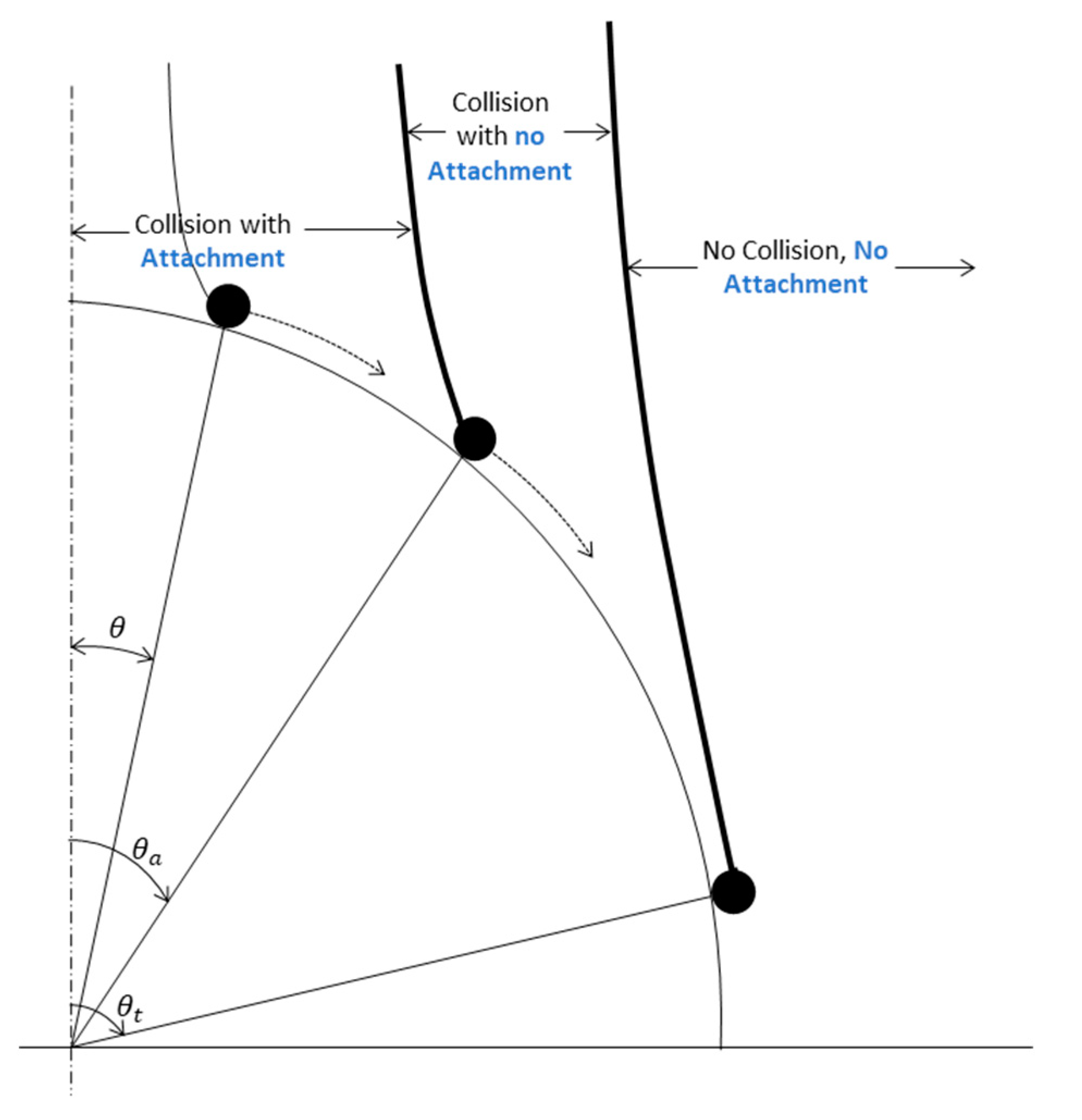
Figure 2 shows the angles involved in particle–bubble interaction (i.e., $\theta$, ${\theta }_{\mathrm{a}}$, and ${\theta }_{\mathrm{t}}$). For a particle to attach to a rising bubble, it must strike with a bubble at a point where its induction time is either equal or greater than the sliding time (induction and sliding time will be discussed in detail in Section 2.1.2). Note that ${\theta }_{\mathrm{a}}$ is an angle where sliding time is just equal to the induction time; however, $\theta$ is an angle (which can be between the vertical axis and the angle ${\theta }_{\mathrm{a}}$) where sliding time is greater than the induction time, so if a particle will strike at any angle $\theta$ up until ${\theta }_{\mathrm{a}}$, it will get attached to the bubble [5,44].

2.1.1. Collision Efficiency ($E_{\mathrm{c}}$)

Particle–bubble collision is the primary and the most important sub-process of flotation that has a significant effect on the flotation rate constant and flotation recovery [11,48,49,50]. The first prediction for the particle–bubble interaction with a mobile bubble surface was proposed by Sutherland [51], who assumed the potential flow around the air bubbles and employed a simplified particle motion equation while neglecting inertial forces due to particle. He simply assumed that particle and bubble size are the main parameters as represented in Equation (2).

$$E_{\mathrm{c}-\mathrm{su}}=\frac{3d_{\mathrm{p}}}{d_{\mathrm{b}}}$$

(2)

As seen in this equation, coarser particles have a better chance of colliding with a bubble, as the calculated collision rate is directly proportional to the particle size.

The Sutherland model was found to overestimate the collision efficiency and has been improved by Dukhin [52] by introducing the inertial forces into the calculations, where it was proposed that the inertial forces have a strong influence on the collision efficiency even when they are weak. Taking into account the approximations of bubble surface mobility, particle size, angle of tangency, hydrodynamic interactions, and inertial forces (both positive and negative), an analytical equation was obtained for the collision efficiency, known as the Generalized Sutherland Equation (GSE) [7,53,54], expressed by Equation (3).

$$E_{\mathrm{c}}=E_{\mathrm{c}-\mathrm{su}}{\sin }^2{\theta }_{\mathrm{t}}\exp \left\{\left[3K_3\left(\ln \frac{3}{E_{\mathrm{c}-\mathrm{su}}}-1.8\right)-\frac{4\left(\frac{2}{3}+\frac{{\cos }^3{\theta }_{\mathrm{t}}}{3}-\cos {\theta }_{\mathrm{t}}\right)}{{\sin }^4{\theta }_{\mathrm{t}}}\right]\cos {\theta }_{\mathrm{t}}\right\}$$

(3)

where ${\theta }_{\mathrm{t}}$ is an angle of tangency (maximum collision angle, shown in Figure 2), expressed as a dimensionless number and described by Equation (4).

$${\theta }_{\mathrm{t}}=\arcsin {\left(2\beta \left(\sqrt{1+{\beta }^2}-\beta \right)\right)}^{\raisebox{1ex}{$1$}\!\left/ \!\raisebox{-1ex}{$2$}\right.}$$

(4)

where the dimensionless number $\beta$ is defined as Equation (5).

$$\beta =\frac{4E_{\mathrm{c}-\mathrm{su}}}{9K_3}$$

(5)

where $E_{\mathrm{c}-\mathrm{su}}$ is defined by Equation (2), and $K_3$ is defined by Equation (6).

$$K_3=\frac{2v_{\mathrm{b}}\left({\rho }_{\mathrm{p}}-{\rho }_{\mathrm{f}}\right)r_{\mathrm{p}}{}^2}{9\mu r_{\mathrm{b}}}$$

(6)

where $v_{\mathrm{b}}$ is a bubble velocity; ${\rho }_{\mathrm{p}}$ and ${\rho }_{\mathrm{f}}$ are particle and fluid densities, respectively; $r_{\mathrm{p}}$ is a particle radius; $\mu$ is a dynamic viscosity of the liquid; and $r_{\mathrm{b}}$ is a bubble radius. Equation (3) along with Equations (4)–(6) were used to calculate the collision efficiency in this study.

2.1.2. Attachment Efficiency $\left(E_a\right)$

The attachment sub-process plays a key role in the aggregation of particle–bubble and its floating transition to the froth zone. It is controlled by particle and bubble surface properties, especially the particle wettability. After a successful collision, a particle slides over the thin liquid film, which forms between the bubble and particle when they come close each other. Later, this film can get thinner and finally reach the critical thickness, leading to the rupture of the film, and then the three-phase contact forms and starts to expand over the particle surface to reach an equilibrium of contact angle on the particle surface [47,55].

Since the early work of Sutherland [51], it has been widely accepted that particle–bubble attachment occurs when the particle–bubble contact time is longer or equal to the induction time [47,56]. The contact time is considered to be the time for which a particle and a bubble are in contact after their collision and is defined as the sum of the impact time and the sliding time. The sliding time is defined as the time taken by a particle to travel from the point of collision to the point where it gets attached to or leaves the bubble surface. The contact time for small-size particles (which possess low mass) mainly refers to the sliding time, since the impact time is much smaller than the sliding time and thus can be approximated to zero [57]. The induction time (t_ind) is defined as the time for the liquid thin film to get thin and rupture, and for the three-phase line of contact to expand until an equilibrium value is obtained [44].

The Dobby–Finch attachment model [45] was used to calculate the attachment efficiency, which is defined as the ratio of the area corresponding to an angle ${\theta }_{\mathrm{a}}$ (adhesion angle) to the area corresponding to ${\theta }_{\mathrm{t}}$ (maximum collision angle, Figure 2). The basic equation for this model is mathematically expressed as Equation (7).

$$E_{\mathrm{a}}=\frac{{\sin }^2{\theta }_{\mathrm{a}}}{{\sin }^2{\theta }_{\mathrm{t}}}$$

(7)

This applies to a particle that collides with the bubble surface at a certain collision angle and then slides along the surface toward the equator of the bubble, for a sliding time which is just equal to the induction time. This particular collision angle is called the adhesion angle (${\theta }_{\mathrm{a}}$) [5,44]. The angle ${\theta }_{\mathrm{a}}$ relates both the sliding and induction times to the attachment efficiency, and can be calculated from Equation (8)

$${\theta }_a=2\times \arctan \times \exp \left[-t_{\mathrm{ind}}\times \frac{2\left(v_{\mathrm{p}}+v_{\mathrm{b}}\right)+v_{\mathrm{b}}{\left(\frac{d_{\mathrm{b}}}{d_{\mathrm{p}}+d_{\mathrm{b}}}\right)}^3}{d_{\mathrm{p}}+d_{\mathrm{b}}}\right]$$

(8)

where $v_{\mathrm{p}}$ is a particle velocity, $v_{\mathrm{b}}$ is a bubble velocity, $d_{\mathrm{p}}$ is a particle diameter, and $d_{\mathrm{b}}$ is a bubble diameter. The induction time ($t_{\mathrm{ind}}$) is related to the particle size and can be expressed by Equation (9) [44]

$$t_{\mathrm{ind}}=A{d}_{\mathrm{p}}^B$$

(9)

where A and B are dimensionless parameters. A is dependent upon particle contact angle and bubble size, whereas B, with a literature value of 0.6, is independent of particle contact angle and bubble size [5,44]. By using experimental data reported by Dai et al. (1999) [44], Koh and Schwarz [58] also proposed the expression shown in Equation (10).

$$t_{\mathrm{ind}}=\frac{75}{\theta }{d}_p^{0.6}$$

(10)

Note that ${\theta }_{\mathrm{t}}$ is a maximum collision angle, which is defined as the angle above which no collision between particle and bubble is possible, and it can be calculated by using Equation (4); however, the dimensionless number $\beta$ in Equation (4) can be expressed as a function of bubble Reynolds number $\left(R_{e\mathrm{b}}\right)$ and is calculated by Equation (11).

$$\beta =\frac{12d_{\mathrm{b}}{\rho }_{\mathrm{f}}}{d_{\mathrm{p}}\left({\rho }_{\mathrm{p}}-{\rho }_{\mathrm{f}}\right)R_{e\mathrm{b}}}$$

(11)

where bubble Reynolds number $\left(R_{e\mathrm{b}}\right)$ is calculated by Equation (12).

$$R_{e\mathrm{b}}=\frac{v_{\mathrm{b}}{d}_{\mathrm{b}}{\rho }_{\mathrm{f}}}{\mu }$$

(12)

Equation (7) together with Equations (4) and (8) and Equations (10)–(12) were used to calculate the attachment efficiency in this study.

2.1.3. Stability Efficiency $\left(E_{\mathrm{s}}\right)$

Particle–bubble stability is controlled by both the attachment forces acting on the bubble–particle aggregate and the external shear stresses in a flotation cell [5]. If the attachment force is greater than the sum of all stress forces, the aggregate remains stable on its way from the pulp phase to the froth phase. The ratio of the detachment forces $\left(F_{\det }\right)$ to the attachment forces $\left(F_{\mathrm{att}}\right)$ characterizes the aggregate stability. This ratio is a dimensionless parameter, the so-called Bond number $B_0^{*}$, and is given by Equation (13) [5].

$$B_0^{*}=\frac{F_{\det }}{F_{\mathrm{att}}}=\frac{F_{\mathrm{g}}-F_{\mathrm{b}}+F_{\mathrm{d}}-F_{ℴ}}{F_{\mathrm{ca}}+F_{\mathrm{hyd}}}$$

(13)

where the forces acting upon the particle are the capillary ($F_{\mathrm{ca}}$), hydrostatic ($F_{\mathrm{hyd}}$), buoyancy ($F_{\mathrm{b}}$), gravitational ($F_{\mathrm{g}}$), machine acceleration ($F_{\mathrm{d}}$), and capillary pressure ($F_{ℴ}$), respectively. The equation for the Bond number can be derived as Equation (14) [5].

$$B_0^{*}=\frac{d_{\mathrm{p}}{}^2\left(\Delta {\rho }_{\mathrm{p}}g+{\rho }_{\mathrm{p}}{a}_{\mathrm{c}}\right)+1.5d_{\mathrm{p}}\left({\sin }^2\omega \right)f\left(d_{\mathrm{b}}\right)}{|6\gamma \left(\sin \omega \right)\left[\sin \left(\omega +\phi \right)\right]|}$$

(14)

With,

$$f\left(d_{\mathrm{b}}\right)=\left(\frac{4\gamma }{d_{\mathrm{b}}}-d_{\mathrm{b}}{\rho }_{\mathrm{f}}g\right)$$

(15)

where $\gamma$ is a surface tension, $a_{\mathrm{c}}$ is a particle centrifugal acceleration in a turbulent flow field, $g$ is a gravitational constant, $\phi$ is a particle contact angle, and $\omega =180°-\frac{\phi }{2}$, which refers to the location of a particle at the liquid–vapor interface. The particle centrifugal acceleration $a_{\mathrm{c}}$ depends on the level of turbulence ($\epsilon$) in the flotation cell, and it can be approximated to Equation (16).

$$a_c=29.6\frac{{\epsilon }^{\raisebox{1ex}{$2$}\!\left/ \!\raisebox{-1ex}{$3$}\right.}}{{\left(d_p+d_b\right)}^{\raisebox{1ex}{$1$}\!\left/ \!\raisebox{-1ex}{$3$}\right.}}$$

(16)

If the bubble–particle aggregate stability efficiency, E_s, is exponentially distributed [8], then E_s can be determined from Equation (17).

$$E_{\mathrm{s}}=1-\exp \left(1-\frac{1}{B_0^{*}}\right)$$

(17)

Equation (17) together with Equations (14)–(16) were used to calculate the stability efficiency in this study.

2.2. Flotation Rate Constant under Turbulent Flow Condition

A general flotation kinetic model was developed for potential flow conditions and is able to calculate the flotation rate constant of particles as a function of particle size as defined in Equation (18).

$$k=2.39\frac{G_f}{d_b{V}_{cell}}\left[\frac{0.33{\epsilon }^{\raisebox{1ex}{$4$}\!\left/ \!\raisebox{-1ex}{$3$}\right.}{d}_b{}^{\raisebox{1ex}{$7$}\!\left/ \!\raisebox{-1ex}{$9$}\right.}}{{\upsilon }^{\raisebox{1ex}{$1$}\!\left/ \!\raisebox{-1ex}{$3$}\right.}}\times {\left(\frac{{\rho }_p-{\rho }_f}{{\rho }_f}\right)}^{\raisebox{1ex}{$2$}\!\left/ \!\raisebox{-1ex}{$3$}\right.}\times \frac{1}{v_b}\right]\times E_c{E}_a{E}_s$$

(18)

where $G_f$ is a gas flow rate, $V_{cell}$ is a flotation cell volume, $\epsilon$ is a turbulence dissipation energy, and $\upsilon$ is a kinematic viscosity. To date, this model equation has been widely accepted [42,59]. Pyke et al., 2003 and Duan et al., 2003 [5,11] reported a good agreement between the model and experimental results for quartz and chalcopyrite particles of diameters ranging from 8 to 100 µm.

2.3. Viscosity Modeling and Factors Affecting Viscosity

Three kinds of forces coexist to various degrees in flowing suspensions: hydrodynamic, Brownian, and colloidal forces [60]. Hydrodynamic (or viscous) forces exist in all flowing suspensions and arise from the relative motion of particles to the surrounding fluid [21]. The Brownian force is the ever-present thermal randomizing force acting on particles suspended in a medium (i.e., liquid or gas). Colloidal forces are potential forces and are elastic in nature [61,62]. The relative magnitude of these forces and, therefore, the bulk rheology depend on the particle size. Brownian motion and interparticle forces quickly equilibrate for sub-micrometer-size suspensions, while hydrodynamic forces dominate for particles larger than approximately 10 μm. For particles in the intermediate range (10⁻³ μm < d < 10¹ μm), the flow behavior is determined by a combination of hydrodynamic forces, Brownian motion, and interparticle forces [6]. The idea of this study is to propose a viscosity equation incorporating those three kinds of forces based on previously suggested equations.

The viscosity of flowing suspensions depends on the shear rate, as well as the characteristics of the continuous phase and the discrete phase. In general, the viscosity of the suspension $\left(\eta \right)$ is directly proportional to the viscosity of the continuous phase, or liquid’s viscosity $\left({\eta }_{\mathrm{L}}\right)$, which can be Newtonian or non-Newtonian. Then, most rheological models are expressed in terms of the relative viscosity of the suspension $\left({\eta }_{\mathrm{r}}\right)$, defined as Equation (19).

$${\eta }_{\mathrm{r}}=\frac{\eta }{{\eta }_{\mathrm{L}}}$$

(19)

2.3.1. Hard Sphere Suspensions

This study begins with the simplest case: suspensions of hard spheres, which are considered to be rigid spherical particles, with no interparticle forces other than infinite repulsion at contact. In other words, there are no attractions or long-range repulsion between the particles.

The viscosity of hard sphere suspensions is affected by viscous forces and Brownian motion. However, Brownian motion is only noticeable for particles smaller than roughly 1 μm [61]. Consequently, hard spheres have been classified as Brownian or non-Brownian, depending on their size [5]. The flow of suspensions of non-Brownian hard spheres is totally dominated by hydrodynamic forces, while Brownian hard spheres interact through both hydrodynamic and Brownian diffusion forces. Brownian hard spheres are non-aggregating colloidal particles.

The hydrodynamic disturbance of the flow field induced by solid particles in a liquid media leads to an increase in the energy dissipation and viscosity [61]. At low solid fraction (in the dilute regime), the relative viscosity of hard-sphere suspensions was first described by the theoretical equation of Einstein, as shown in Equation (20).

$${\eta }_{\mathrm{r}}=1+\left[\eta \right]\varphi$$

(20)

where $\varphi$ and $\left[\eta \right]$ are the solid fraction and the viscosity of the dispersion medium, respectively. At higher concentrations, particles crowding produces hydrodynamic interactions (as well as increasing probability of collision) between particles, resulting in significant positive deviations from Equation (20). Many models have been proposed to describe the concentration dependence of the relative viscosity of concentrated suspensions. One of the most useful expressions is the semi-empirical equation of Krieger and Dougherty for monodisperse suspensions, Equation (21).

$${\eta }_{\mathrm{r}}={\left(1-\frac{\varphi }{{\varphi }_m}\right)}^{-\left[\eta \right] {\varphi }_m}$$

(21)

where $\left({\varphi }_m\right)$ is the maximum packing fraction of particles. As particle concentration approaches the level corresponding to a dense packing of particles $\left({\varphi }_m\right)$, there is no longer sufficient fluid to lubricate the relative motion of particles, and the viscosity rises to infinity. Although the theoretical $\left({\varphi }_m\right)$ value of monodisperse spheres is 0.74 (in a face-centered cubic (FCC) array), experimental observations have shown that loose random packing is close to 0.60, and that dense random packing (or random close packing (RCP)) is close to 0.64. Practical experience shows that the product $\left[\eta \right] {\varphi }_m$ in Equation (21) is often around 2 for a variety of situations. Then, Krieger and Dougherty’s equation is usually simplified to Equation (22) [63,64].

$${\eta }_{\mathrm{r}}={\left(1-\frac{\varphi }{{\varphi }_m}\right)}^{-2}$$

(22)

2.3.2. Effect of Shear Rate

At low particle concentrations, the viscosity of hard sphere suspensions (Equation (20)) is independent of shear rate ($\stackrel{.}{\gamma }$). At higher concentrations, the viscosity exhibits a typical three-stage dependence with shear rate: (1) at low shear rates, they show Newtonian behavior, with a constant zero-shear viscosity $\left({\eta }_0\right)$; (2) at intermediate shear rates, the viscosity decreases following a shear-thinning behavior (a phenomenon characteristic of some non-Newtonian fluids in which the fluid viscosity decreases with increasing shear stress); and (3) at high shear rates, the viscosity attains a limiting and constant value, the infinite-shear viscosity $\left({\eta }_{\infty }\right)$. The decrease in viscosity at increasing shear rates is either due to the alignment of suspended particles in the direction of flow or to the shear thinning behavior of the suspending liquid (the continuous phase) [65].

In the case of Brownian hard spheres, viscous forces disturb the microstructure against the restoring effect of Brownian motion. In the low-shear-rate regime, Brownian diffusion predominates over hydrodynamic interactions, and the suspension shows a high viscosity $\left({\eta }_0\right)$ due to the random arrangement of particles. Inversely, in the high-shear-rate regime, hydrodynamic forces predominate over Brownian diffusion, and the layers of particles can move freely past each other, giving a low viscosity $\left({\eta }_{\infty }\right)$. Both ${\eta }_0$ and ${\eta }_{\infty }$ increase uniformly with solid fraction, and shear thinning is only detectable for $\varphi >0.25-0.30$ and only substantial for $\varphi >0.5$ [66]. This rheological behavior was originally described by a simple model developed by Krieger and Dougherty [67], where the apparent viscosity depends on ${\eta }_0$, ${\eta }_{\infty }$, and the shear stress [68,69]. In the modified Krieger and Dougherty model, the Brownian and hydrodynamic effects can be properly scaled by plotting the viscosity of the suspension as a function of the dimensionless Peclet number, instead of the shear rate or the shear stress. The Peclet number is defined as the ratio of the hydrodynamic to the thermal force and can be calculated as Equation (23).

$$Pe=\frac{6\pi a^3{\eta }_L\stackrel{.}{\gamma }}{k_{\mathrm{B}}T}$$

(23)

where $a$ is a radius of hard sphere, $k_{\mathrm{B}}$ is Boltzmann’s constant, and $T$ is an absolute temperature. The relative viscosity of Brownian hard-sphere suspensions can be properly described by this model in terms of the Peclet number, as Equation (24).

$${\eta }_{\mathrm{r}}={\eta }_{\mathrm{r}\infty }+\frac{{\eta }_{\mathrm{r}0}-{\eta }_{\mathrm{r}\infty }}{1+{\left(\raisebox{1ex}{$Pe$}\!\left/ \!\raisebox{-1ex}{$P{e}_c$}\right.\right)}^n}$$

(24)

where $n=1$ for monodisperse suspensions, and the fitting parameter $P{e}_c$ is a characteristic Peclet number, which depends on the volume fraction of particles [21]. Expressions for ${\eta }_{\mathrm{r}0}\left(\varphi \right)$ and ${\eta }_{\mathrm{r}\infty }\left(\varphi \right)$ can be obtained by replacing ${\varphi }_{m0}\approx 0.63$ and ${\varphi }_{m\infty }\approx 0.71$ into Equation (22), respectively.

2.3.3. Colloidal Suspensions

Colloidal suspensions may be defined as biphasic systems where the discrete phase is subdivided into elemental units (particles/droplets) that are large compared to simple molecules, but small enough so that interparticle forces are significant in governing system properties. The size of colloidal particles is typically considered to be from a few nanometers to a few micrometers [62].

In the colloidal particles, the interactions are controlled by a range of attractive and repulsive interparticle forces [70]. DLVO theory is one of the best-known theories for describing the particle–particle interactions with the summation of the van der Waals potential $\left(V_{VDW}\right)$ and electrical double-layer potential $\left(V_{EDL}\right)$ [32,71]. If the total potential energy $\left(V_T=V_{VDW}+V_{EDL}\right)$ is high and positive, particles repel each other; otherwise, particles attract each other. This is a straightforward theory that can explain particle coagulation/dispersion in different colloidal systems [72,73,74,75,76]. The following paragraphs will introduce and explain the equations used for the potential energy calculation.

Equations used to calculate the potential energies between similar particles are as below [32]:

$$V_A=-\frac{Aa}{12H}$$

(25)

$$H=\left\{{\left( \frac{0.52}{\varphi }\right)}^{\raisebox{1ex}{$1$}\!\left/ \!\raisebox{-1ex}{$3$}\right.}-1\right\}\times D$$

(26)

$$V_R=\frac{64\pi an{k}_{B}T{\gamma }^2\exp \left(-\kappa H\right)}{{\kappa }^2}$$

(27)

$$n=N_{A}C$$

(28)

$$\kappa ={\left(\frac{2n{z}^2{e}^2}{\epsilon {\epsilon }_0{k}_{B}T}\right)}^{\raisebox{1ex}{$1$}\!\left/ \!\raisebox{-1ex}{$2$}\right.}$$

(29)

$$\gamma =\frac{e^{\left(\frac{ze\zeta }{2k_{B}T}\right)}-1}{e^{\left(\frac{ze\zeta }{2k_{B}T}\right)}-1}$$

(30)

where $A$ is the Hamaker constant, $a$ is the particle radius, $H$ is the interparticle separation distance defined by solid fraction $\varphi$ and particle diameter D in this study (Equation (26)), $n$ is the number concentration of ions (defined in Equation (28)), $N_A$ is the Avogadro’s number, $C$ is the concentration of ions, $\kappa$ is the Debye–Huckel reciprocal length (defined in Equation (29)), $\gamma$ is the reduced surface potential (unitless, defined in Equation (30)), $z$ is the ionic valence, $e$ is the elementary charge, $\epsilon$ is the dielectric constant of the medium, ${\epsilon }_0$ is the permittivity of free space, and $\zeta$ is the zeta potential. In this study, Equation (26) was applied in order to determine a certain value of H for the specific $\varphi$ and D and to perform the viscosity calculation by using Equation (33).

Equations used to calculate the potential energies between similar particles but different particle sizes are as below [77]:

$$V_A=-\frac{A{a}_1{a}_2}{6\left(a_1+a_2\right)H}$$

(31)

$$V_R=\frac{{\epsilon }_0\epsilon a_1{a}_2\left({\zeta }_1^2+{\zeta }_2^2\right)}{4\left(a_1+a_2\right)}\times \left[\left\{\frac{2{\zeta }_1{\zeta }_2}{\left({\zeta }_1^2+{\zeta }_2^2\right)}\times ln\left(\frac{1+e^{-\kappa H}}{1-e^{-\kappa H}}\right)\right\}+ln\left(1-e^{-2\kappa H}\right)\right]$$

(32)

The equation we propose in this study to calculate the relative viscosity is Equation (33), incorporating a combination of hydrodynamic forces, Brownian motion, and interparticle forces, and later on, Equation (19) was used to calculate the viscosity of the suspension $\left(\eta \right)$.

$${\eta }_r={\eta }_{r\infty }+\frac{{\eta }_{r0}-{\eta }_{r\infty }}{1+{\left(\raisebox{1ex}{$Pe$}\!\left/ \!\raisebox{-1ex}{$P{e}_c$}\right.\right)}^n}+k_1{\eta }_L\varphi \exp \left(\frac{V_T}{k_{B}T}\right)$$

(33)

3. Results and Discussion

This section is composed of two parts. The Section 3.1 and Section 3.2 will first illustrate and discuss the effect of particle size and suspension viscosity on the flotation efficiencies and rate constant of the particle size range between 8 and 100 µm based on the previously proposed equations. The Section 3.3 and Section 3.4 will then show and discuss the suspension viscosity calculated by viscosity model equations and their integration to the flotation efficiencies and rate constant model that are now able to calculate and investigate the effect of the solid concentration/fraction and shear rate on flotation efficiencies and rate constant of selected flotation particle size of 80 µm. Literature values summarized in Table 1 were used to compare with our calculated values. The suspension viscosity calculation results presented in this section were made on quartz particle suspensions, using the liquid viscosity of water at 25 °C as 0.00091 Pa s [78], suspension pH as 10, and salt concentration and type as 1 × 10⁻² M KNO₃, respectively. pH 10 is a typical pH for quartz flotation [79]. The zeta potential value of quartz particle was extracted from our previous report [80]. After our preliminary calculations (Appendix A Figure A1, presented in Section 3.1), the flotation efficiencies and rate constant were calculated using the calculated suspension viscosity and for the following conditions: turbulence dissipation energy $\epsilon =10$ m² s⁻³, gas flow rate as 0.0035 m³ min⁻¹, bubble diameter as 0.0014 m, volume of cell as 0.00225 m³, quartz particle density as 2650 kg/m³, bubble velocity as 0.18 m s⁻¹, liquid–vapor surface tension as 72.8 m Nm⁻¹, particle contact angle as 80°, and flotation particle diameter as 80 μm [5].

3.1. Calculated Flotation Collection Efficiencies $E_{\mathrm{c}}$, $E_{\mathrm{a}}$, $E_{\mathrm{s}}$, and Rate Constant $k$

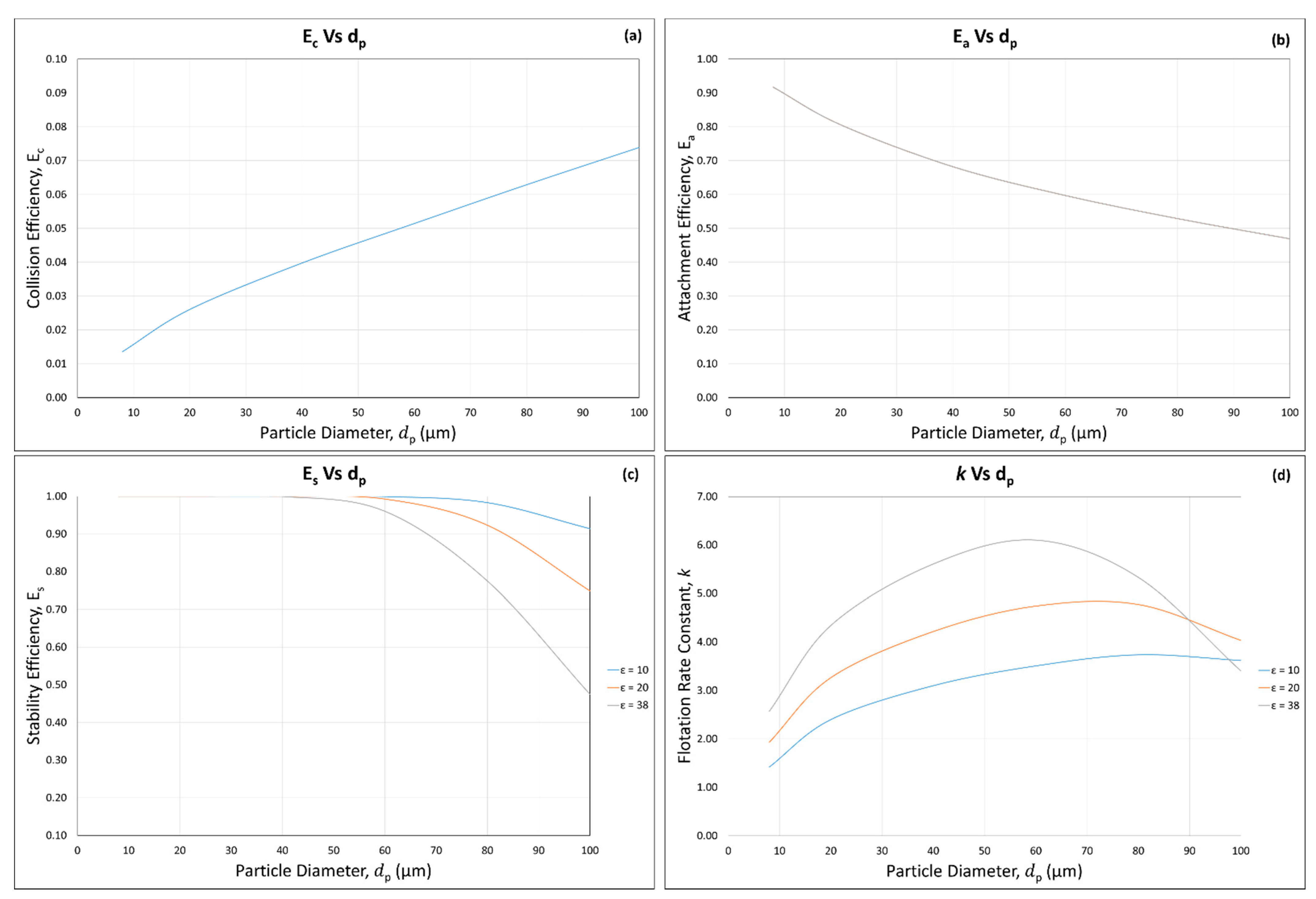
Appendix A Figure A1 shows results for calculated collision $\left(E_{\mathrm{c}}\right)$, attachment $\left(E_{\mathrm{a}}\right)$, and stability $\left(E_{\mathrm{s}}\right)$ efficiencies and flotation rate constant, $k$, using Equations (3), (7), (17) and (18), respectively, as a function of particle diameter. It can be seen that $E_{\mathrm{c}}$ increases with an increase in particle diameter, while both $E_{\mathrm{a}}$ and $E_{\mathrm{s}}$ decrease with increasing particle size. The combination of these efficiencies in Equation (18) produced the characteristic shape of the flotation rate constant versus particle size curve, with a maximum value obtained at intermediate particle size (60–80 µm). The low values of flotation rate constants obtained on each side of this maximum are due to low collision efficiencies for fine particles and low attachment and stability efficiencies for coarse particles, as discussed in literature and our recent review article [5,6].

Appendix A Figure A1 also shows the effect of dissipation energy on these efficiencies and flotation rate constant. With increasing dissipation energy (ε), $E_{\mathrm{s}}$ decreases as a result of a larger acceleration force on the particle–bubble aggregate as increasing ε plays a role of detachment force, while the flotation rate constant increases because of increased particle–bubble collision frequency. Pyke et al. (2003) [5] reported an agreement with the quartz particles with an advancing water contact angle of 80° interacting with gas bubbles 1.4 × 10⁻³ m in diameter introduced at a gas flow rate of 3.5 × 10⁻³ m³ min⁻¹ and at an agitation speed of 650 rpm in a Rushton flotation cell. According to them, the best fit of the experimental and calculated flotation rate constant was obtained with a fluid velocity of 0.18 ± 0.01 ms⁻¹ and a dissipation energy of 38 ± 7 m² s⁻³ (95% confidence limits).

3.2. Effect of Suspension Viscosity on $E_{\mathrm{c}}$, $E_{\mathrm{a}}$, $E_{\mathrm{s}}$, and Rate Constant $k$

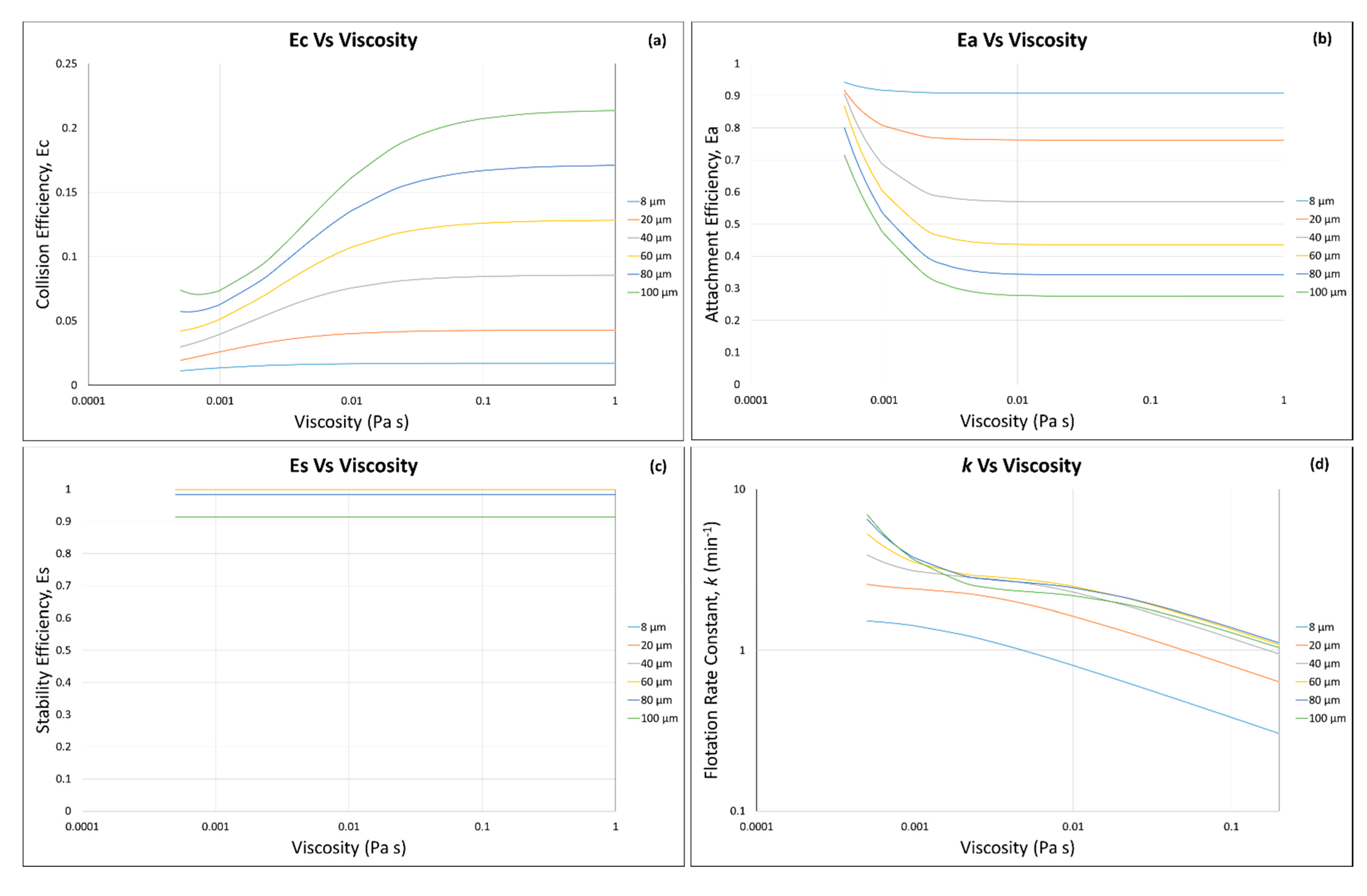
Suspension viscosity was varied between 0.0005 and 1 Pa s, and the flotation efficiencies and rate constant were calculated by using the flotation kinetics model introduced in Section 2 as a function of particle diameter (8–100 µm). The results shown in Figure 3a indicate that the increase in viscosity increases the collision efficiency $\left(E_{\mathrm{c}}\right)$ with the greater particle diameter. The increase in suspension viscosity decreases the Stokes number (Equation (6)), which in turn increases the maximum collision angle (${\theta }_{\mathrm{t}}$) (Equation (4)). As shown in Figure 2, a higher ${\theta }_{\mathrm{t}}$ means a higher collision probability between particle and bubble. With the increase in particle size, the probability of collision between bubble and particle increases (as explained by the Sutherlands [51] (Equation (2)), and thus the collision efficiency increases with the increase in particle diameter.

The attachment efficiency $\left(E_{\mathrm{a}}\right)$ decreases with an increase in the suspension viscosity and particle diameter. In other words, the higher the particle diameter, the lower the attachment efficiency. On the other hand, $E_{\mathrm{a}}$ becomes constant above a certain suspension viscosity (around above 0.008 Pa s) regardless of the particle size (Figure 3b). Schubert (2008) [81] argued that low pulp viscosity causes a reduction in turbulence damping, which increases the probability of particle–bubble attachment. The increase in suspension viscosity decreases the bubble Reynolds number (Equation (12)), which in turn increases the maximum collision angle (${\theta }_{\mathrm{t}}$) (Equation (4)), and as shown in Equation (7), a higher ${\theta }_{\mathrm{t}}$ reduces the attachment efficiency.

Stability efficiency $\left(E_{\mathrm{s}}\right)$ remained unaffected by the change in suspension viscosity as it varies with the change in turbulence dissipation energy $\left(\epsilon \right)$, particle diameter $\left(d_{\mathrm{p}}\right)$, and bubble diameter $\left(d_{\mathrm{b}}\right)$ (Equation (16)) [82]. As $\epsilon$ and $d_{\mathrm{b}}$ remained constant throughout the study, the decrease in $E_{\mathrm{s}}$ from 1 to 0.91 corresponds with the increase in particle size from 60 to 100 µm, respectively (Figure 3c). This decrease can be explained by the fact that the larger particles have higher mass, and therefore their probability to successfully reach to the concentrate through the pulp phase via particle–bubble aggregate becomes lower than that of smaller particles, as seen in the Bond number (Equation (14)).

The increasing suspension viscosity decreases the flotation rate constant ($k$), with the maximum value of 3.97 min⁻¹ at 80 µm and 0.0009 Pa s. The $k$ decreased above the viscosity value 0.0009 Pa s (Figure 3d). However, the value of $k$ increases below 0.00091 Pa s, that is, the viscosity of water at 25 °C [78]. Therefore, considering water is used in flotation operations, 0.00091 Pa s was selected to calculate the maximum value of $k$. This also agrees with the study performed by Pyke et al. (2003) [5] and Duan et al. (2003) [11] who reported the optimum flotation rate constant of 7 min⁻¹ with the quartz particles with an advancing water contact angle of 80° interacting in a Rushton flotation cell with gas bubbles 1.4 × 10⁻³ m in diameter introduced at a gas flow rate of 3.5 × 10⁻³ m³ min⁻¹ and at an agitation speed of 650 rpm. Chen et al. (2017) [18] reported the decrease in copper flotation recovery from 95 to 63.6% with an increase in pulp viscosity from 0.109 to 0.147 Pa s in the presence of 30 vol.% and 50 vol.% of amorphous silica in a suspension of the mixture of amorphous silica and quartz, respectively. This agrees with the $k$ calculated and shown in Figure 3d, and $k$ decreased from 1.347 to 1.227 min⁻¹ with increase in the suspension viscosity from 0.109 to 0.147 Pa s. As seen in Figure 3d, k is more affected by $E_{\mathrm{a}}$ since the magnitude of $E_{\mathrm{a}}$ is higher than $E_{\mathrm{c}}$, while $E_{\mathrm{s}}$ remain unchanged.

It should also be noted that the flotation kinetics model is limited to the use of suspension viscosity as low as 0.0005 Pa s. Below this value of suspension viscosity, the flotation efficiencies and rate constant are overestimated and thus not plotted in Figure 3.

The results presented in this section clearly illustrate the effect of particle size and suspension viscosity on the flotation efficiencies and rate constant. The following Section 3.3 and Section 3.4 will then show and discuss the effect of the solid concentration/fraction and shear rate on the suspension viscosity and then flotation efficiencies and rate constant by using/developing viscosity model equations that were coupled with flotation efficiencies and rate constant models for the first time.

3.3. Suspension Viscosity Calculation

3.3.1. Modified Krieger and Dougherty Model—Hard Sphere Suspensions

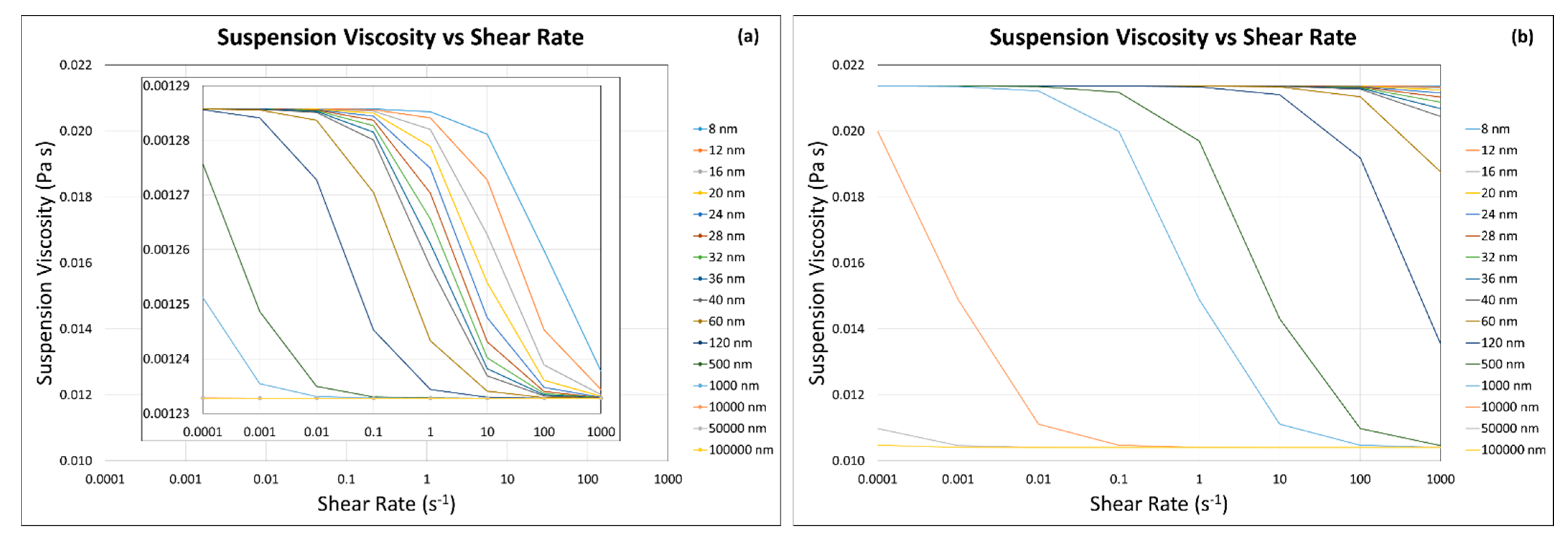
The suspension viscosity was calculated using Equations (24) and (19) for quartz as particles. The results are shown in Figure 4, and it can be seen that the suspension viscosity decreases with an increase in shear rate, at both solid fractions (i.e., $\varphi =0.1$ and $0.5$). With the increase in solid fraction, there is a significant increase in suspension viscosity. The suspension viscosity increases with the decrease in ultrafine particle size (i.e., 1 µm–8 nm) at both particle fractions.

In the smaller solid fraction ($\varphi =0.1$, Figure 4a), at smaller particle size (i.e., 8 nm–1 µm), the effect of shear rate on decreasing the suspension viscosity is significant because the thermal diffusion is more dominant than the hydrodynamic forces. On the other hand, above 1 µm, the effect is very limited because the hydrodynamic forces are quite dominant as compared with the thermal diffusion at lower solid fraction ($\varphi =0.1)$ compared with the high solid fraction ($\varphi =0.5$) [21].

In the higher solid fraction ($\varphi =0.5$, Figure 4b), at smaller particle size (i.e., 8 nm–40 nm), the effect of shear rate on decreasing suspension viscosity is very limited because the thermal diffusion is more dominant than the hydrodynamic forces [21]. At the intermediate ultra-fine particle size (i.e., 60 nm–10 µm), the effect of shear rate on the decreasing suspension viscosity is more significant because the hydrodynamic forces are more dominant as compared with the thermal diffusion with increasing shear rate. At above the intermediate particle sizes (i.e., 50 µm), the effect of shear rate on the suspension viscosity again becomes very limited because the hydrodynamic forces are dominant regardless of the shear rate.

3.3.2. Our Predictive Model—Hard Sphere and Interacting Colloidal Particle Suspensions

Homogeneous Case (i.e., Same Particle with Same Sizes)

The suspension viscosity was calculated using Equations (33) and (19) for the same quartz particles with the same sizes. Figure 5 shows the calculated suspension viscosity for the homogeneous case (i.e., same particles with same sizes) at $\varphi =0.1$ and $0.3$. It can be seen in Figure 5a,b that with the increase in solid fraction from $\varphi =0.1$ to $0.3$, there is significant increase in suspension viscosity (0.00123–0.00128 Pa s to 0.00272–0.00331) because the total potential energy increases with the increase in $\varphi$ [21]. Chen et al. (2017) [18] discussed a similar trend of increase in suspension viscosity with the increase in solid concentration and reported the apparent viscosity of amorphous silica and quartz suspension increased from 0.109 to 0.147 Pa s with the increase in the concentration of amorphous silica (in the mixture of amorphous silica and quartz suspension) from 30 to 50 vol.%, at a shear rate of 100 s⁻¹. Schubert (1999) [81] reported that the suspensions containing higher percent of solids produce higher slurry viscosity, particularly in the case of interacting particles. Ndlovu et al. (2011) [83] reported an increase in the suspension viscosity from 0.010 to 0.074 Pa s with an increase in the solid concentration from 25 to 35 vol.% (62.5 to 87.5 wt.%) of pure vermiculite, respectively. They also reported an increase in the suspension viscosity from 0.011 to 0.023 Pa s with an increase in the solid concentration from 30 to 35 vol.% (79.5 to 92.75 wt.%) of pure quartz, respectively.

Table 2. DLVO total potential energies between two quartz particles at different solid fractions and particle sizes for the same quartz particles with the same particle sizes.

ϕ/a	8 (nm)	12 (nm)	16 (nm)	20 (nm)	24 (nm)	28 (nm)	32 (nm)	36 (nm)	40 (nm)	60 (nm)	120 (nm)	500 (nm)	1000 (nm)	10,000 (nm)	50,000 (nm)	100,000 (nm)
0.1	3.36	1.91	1.31	1.07	9.70 × 10−1	9.26 × 10−1	9.06 × 10−1	8.98 × 10−1	8.94 × 10−1	8.92 × 10−1	8.92 × 10−1	8.92 × 10−1	8.92 × 10−1	8.92 × 10−1	8.92 × 10−1	8.92 × 10−1
0.176	1.51 × 101	9.63	5.24	3.04	1.99	1.47	1.20	1.05	9.57 × 10−1	8.35 × 10−1	8.24 × 10−1	8.24 × 10−1	8.24 × 10−1	8.24 × 10−1	8.24 × 10−1	8.24 × 10−1
0.2	2.40 × 101	1.80 × 101	1.01 × 101	5.53	3.30	2.19	1.62	1.30	1.11	8.33 × 10−1	7.99 × 10−1	7.99 × 10−1	7.99 × 10−1	7.99 × 10−1	7.99 × 10−1	7.99 × 10−1
0.3	1.42 × 102	3.19 × 102	3.69 × 102	2.85 × 102	1.76 × 102	9.81 × 101	5.30 × 101	2.91 × 101	1.67 × 101	2.39	6.91 × 10−1	6.59 × 10−1	6.59 × 10−1	6.59 × 10−1	6.59 × 10−1	6.59 × 10−1
0.4	5.20 × 102	5.55 × 103	3.16 × 104	1.07 × 105	2.39 × 105	3.78 × 105	4.54 × 105	4.38 × 105	3.57 × 105	3.12 × 104	1.63 × 101	3.99 × 10−1	3.99 × 10−1	3.99 × 10−1	3.99 × 10−1	3.99 × 10−1
0.5	1.13 × 101	7.41 × 102	4.18 × 104	2.05 × 106	8.72 × 107	3.25 × 109	1.06 × 1011	3.05 × 1012	7.73 × 1013	1.40 × 1020	3.80 × 1032	4.60 × 1025	5.73 × 103	1.69 × 10−3	1.69 × 10−3	1.69 × 10−3

shows the calculations of the DLVO total potential energies at different solid fractions as a function of ultra-fine particle sizes. At higher solid fractions (i.e., $\varphi =0.4$ and $0.5$), the values of total potential energy become very high (>5 × 10³, Table 2) due to the decrease in interparticle distance (Equation (26)), which results in abnormal values of suspension viscosity. On the other hand, for the lower solid fractions (i.e., $\varphi$ ≤ 0.3) and the case of same quartz particles with same particle sizes, the DLVO calculations result in acceptable total potential energies and were thus applied in the calculations of suspension viscosities as well as flotation efficiencies and rate constants.

Homogeneous Case (i.e., Same Particles with Different Particle Sizes)

The suspension viscosity was calculated using Equations (33) and (19) (for same quartz particles with different sizes). In all these calculations, the coarse particle size was kept constant (i.e., 80 µm), and the suspension viscosity was calculated for four different scenarios (Figure 6). They are the suspension containing (a) 90 vol.% coarse particles ($a_1$) and 10 vol.% ultra-fine/fine particles ($a_2$) at $\varphi =0.1$, (b) 10 vol.% coarse particles ($a_1$) and 90 vol.% ultra-fine/fine particles ($a_2$) at $\varphi =0.1$, (c) 10 vol.% coarse particles ($a_1$) and 90 vol.% ultra-fine/fine particles ($a_2$) at $\varphi =0.5$, and (d) 90 vol.% coarse particles ($a_1$) and 10 vol.% ultra-fine/fine particles ($a_2$) at $\varphi =0.5$. Here, coarse particle refers to the mechanical flotation size particle (i.e., 80 µm selected from Appendix A Figure A1), and we intend to study the effect of the presence of ultra-fine/fine particles on the viscosity of coarse and ultra-fine/fine particle mixture suspension (Figure 6) and then the flotation efficiencies and rate constant of coarse particle (Section 3.4.2).

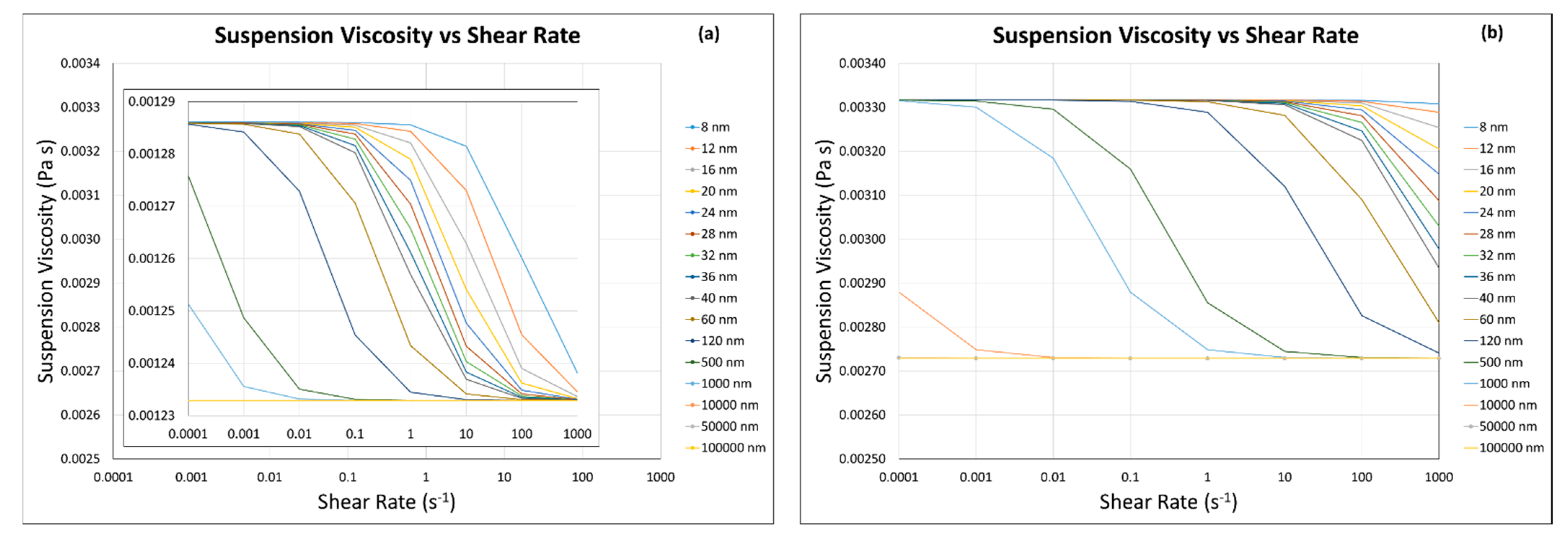
It can be seen that the presence of more ultrafine particles (90 vol.%) increases the suspension viscosity at lower shear rate (<0.001 s⁻¹) at both solid fractions ($\varphi =0.1$ and $0.5$). The increase in the suspension viscosity was more at higher solid fraction ($\varphi =0.5$, Figure 6c) as compared with the lower solid fraction ($\varphi =0.1$, Figure 6a). This was obvious because particles crowding enhances thermal diffusion and colloidal interactions, and the suspension shows a high viscosity at low shear rate (≤0.001 s⁻¹), while it decreased and becomes constant due to the domination of hydrodynamic interactions at higher shear rate (>0.001 s⁻¹). Genovese [21] discussed the similar behavior of interacting particles and reported that the suspension viscosity decreased significantly from 0.2548 to 0.00254 Pa s between varied shear rates from 0.01 to 1000 s⁻¹ when the solid fraction $\left(\varphi \right)$ was 0.345. Schubert (1999) [81] also reported that suspensions containing a higher percent of solids produce higher slurry viscosity, particularly in the case of interacting particles.

When the presence of fine/ultra-fine particles was low (=10 vol.%), shear rate showed an almost negligible effect on the change in suspension viscosity at both solid fractions ($\varphi =0.1$ and $0.5$, Figure 6b,d). The suspension viscosity was least affected even at the low shear rates (Figure 6b,d). Genovese [21] discussed the similar behavior of interacting particles and reported that the suspension viscosity remained almost constant (i.e., 0.00099 Pa s) at different shear rates, varying from 0.01 to 1000 s⁻¹, when the solid fraction $\left(\varphi \right)$ was as low as 0.176. With the higher solid fraction ($\varphi =0.5$), there is a slight increase (2%) in the suspension viscosity at the lowest shear rate (0.0001 s⁻¹), possibly due to thermal diffusion and colloidal interactions enhanced by many particle systems (Figure 6d).

From these results, it can be deduced that the presence of little amount of fine/ultra-fine particles in the suspension of coarse and fine/ultra-fine particles (e.g., $a_1:a_2=9:1$) has an almost negligible effect on the suspension viscosity at low solid fraction (i.e., $\varphi =0.1$) (Figure 6b). Even at higher solid fraction ($\varphi =0.5$), the effect on the suspension viscosity remains negligible (other than at very low shear, as discussed earlier) (Figure 6d). Contrary to this, the large amount of fine/ultra-fine particles in the suspension of coarse and fine/ultra-fine particles (e.g., $a_1:a_2=1:9$) has a limited effect on the suspension viscosity (0.00123289 to 0.00123295 Pa) at low solid fraction (i.e., $\varphi =0.1$) (Figure 6a). At the higher solid fraction ($\varphi =0.5$), the effect of fine/ultra-fine particles on the suspension viscosity becomes very significant (0.01048 to 0.02061 Pa s), and this can be observed by the magnitude of the suspension viscosity, which lies between 0.01 to 0.02 Pa s (100% increase, Figure 6c).

Table 3. DLVO total potential energies between coarse (80 µm) and fine/ultra-fine particles at different solid fractions and particle sizes for the same quartz particles with different particle sizes.

ϕ/a	8 (nm)	12 (nm)	16 (nm)	20 (nm)	24 (nm)	28 (nm)	32 (nm)	36 (nm)	40 (nm)	60 (nm)	120 (nm)	500 (nm)	1000 (nm)	10,000 (nm)	50,000 (nm)	100,000 (nm)
0.1	9.98 × 10−1	9.97 × 10−1	9.97 × 10−1	9.96 × 10−1	9.96 × 10−1	9.96 × 10−1	9.95 × 10−1	9.95 × 10−1	9.95 × 10−1	9.94 × 10−1	9.91 × 10−1	9.82 × 10−1	9.75 × 10−1	9.30 × 10−1	8.94 × 10−1	8.92 × 10−1
0.176	9.96 × 10−1	9.95 × 10−1	9.95 × 10−1	9.94 × 10−1	9.93 × 10−1	9.93 × 10−1	9.92 × 10−1	9.92 × 10−1	9.91 × 10−1	9.89 × 10−1	9.85 × 10−1	9.70 × 10−1	9.58 × 10−1	8.86 × 10−1	8.29 × 10−1	8.25 × 10−1
0.2	9.96 × 10−1	9.95 × 10−1	9.94 × 10−1	9.93 × 10−1	9.92 × 10−1	9.92 × 10−1	9.91 × 10−1	9.91 × 10−1	9.90 × 10−1	9.88 × 10−1	9.83 × 10−1	9.65 × 10−1	9.52 × 10−1	8.69 × 10−1	8.04 × 10−1	8.00 × 10−1
0.3	9.92 × 10−1	9.90 × 10−1	9.88 × 10−1	9.87 × 10−1	9.86 × 10−1	9.85 × 10−1	9.83 × 10−1	9.82 × 10−1	9.82 × 10−1	9.77 × 10−1	9.68 × 10−1	9.37 × 10−1	9.12 × 10−1	7.69 × 10−1	6.66 × 10−1	6.60 × 10−1
0.4	9.82 × 10−1	9.78 × 10−1	9.74 × 10−1	9.71 × 10−1	9.69 × 10−1	9.66 × 10−1	9.64 × 10−1	9.62 × 10−1	9.60 × 10−1	9.51 × 10−1	9.31 × 10−1	8.66 × 10−1	8.16 × 10−1	5.61 × 10−1	4.09 × 10−1	4.01 × 10−1
0.5	9.27 × 10−1	8.87 × 10−1	8.56 × 10−1	8.32 × 10−1	8.12 × 10−1	7.95 × 10−1	7.80 × 10−1	7.67 × 10−1	7.54 × 10−1	7.06 × 10−1	6.10 × 10−1	3.67 × 10−1	2.44 × 10−1	1.81 × 10−2	2.01 × 10−3	1.76 × 10−3

shows the calculations of the DLVO total potential energies between an 80 µm particle and a fine/ultra-fine particle at different solid fractions as a function of fine/ultra-fine particle sizes. The increase in solid fractions (i.e., $\varphi =0.1$ to $0.5$) causes a decrease in total potential energy, meaning stronger attractive interaction between two particles. For example, the total potential energy between ultra-fine particle size of 8 nm and coarse particle size of 80 µm decreased from 9.98 × 10⁻¹ to 9.27 × 10⁻¹ with an increase in solid fraction from 0.1 to 0.5. The reason behind this decrease is that with the increase in solid fraction, interparticle distance (Equation (26)) decreases, resulting in stronger van der Walls attraction. Similarly, behavior can be seen with the increase in fine/ultra-fine particle size (8 nm to 100 µm); for example, with the increase in fine/ultra-fine particle size (8 nm to 100 µm) at solid fraction 0.1, the total potential energy decreased from 9.98 × 10⁻¹ to 8.92 × 10⁻¹. The DLVO calculations shown in Table 3 were thus applied in the calculations of suspension viscosities as well as flotation efficiencies and rate constants.

3.4. Flotation Efficiencies and Rate Constant Calculations

3.4.1. Incorporation of the Modified Krieger and Dougherty Model—Hard Sphere Suspensions

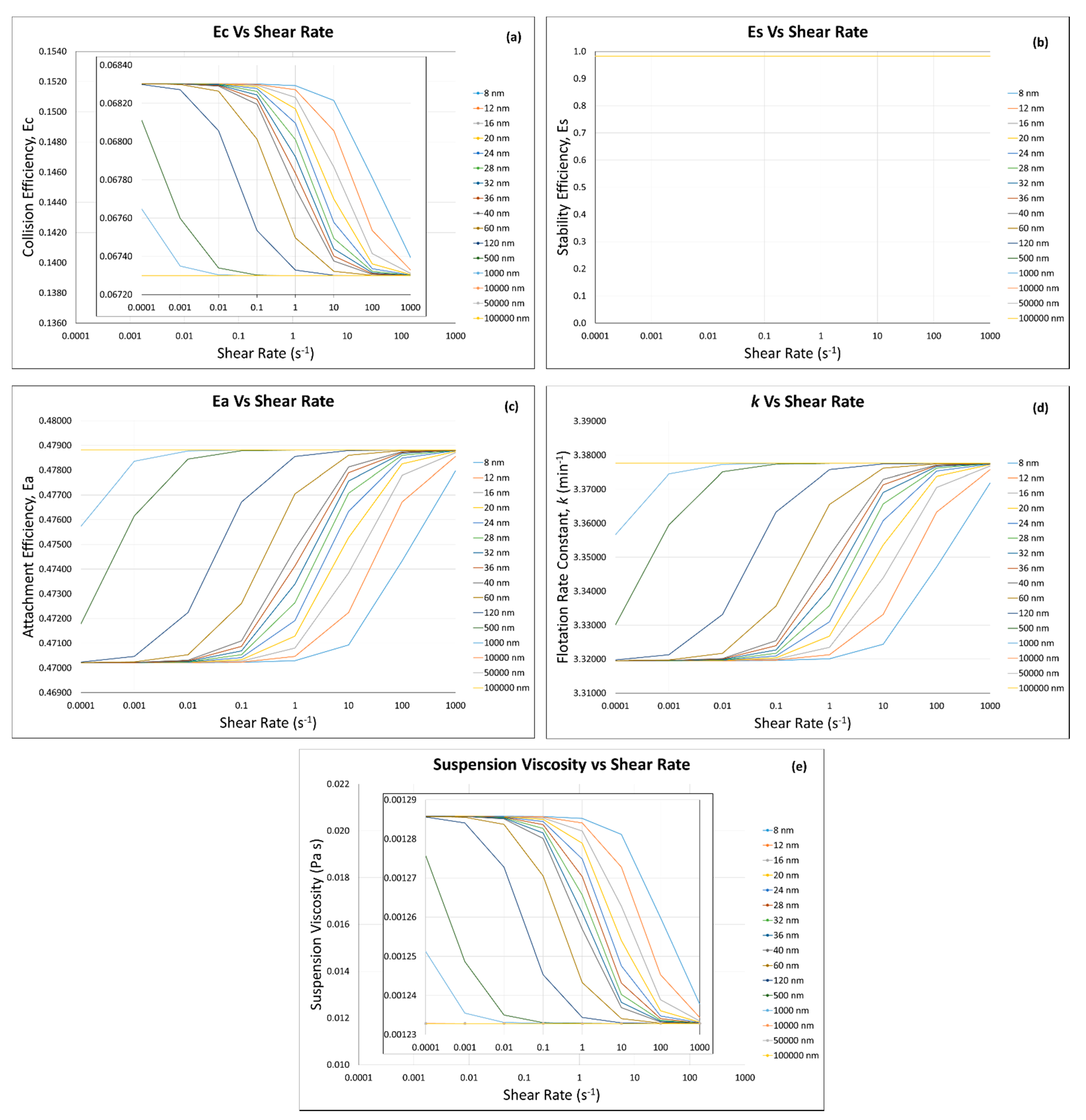
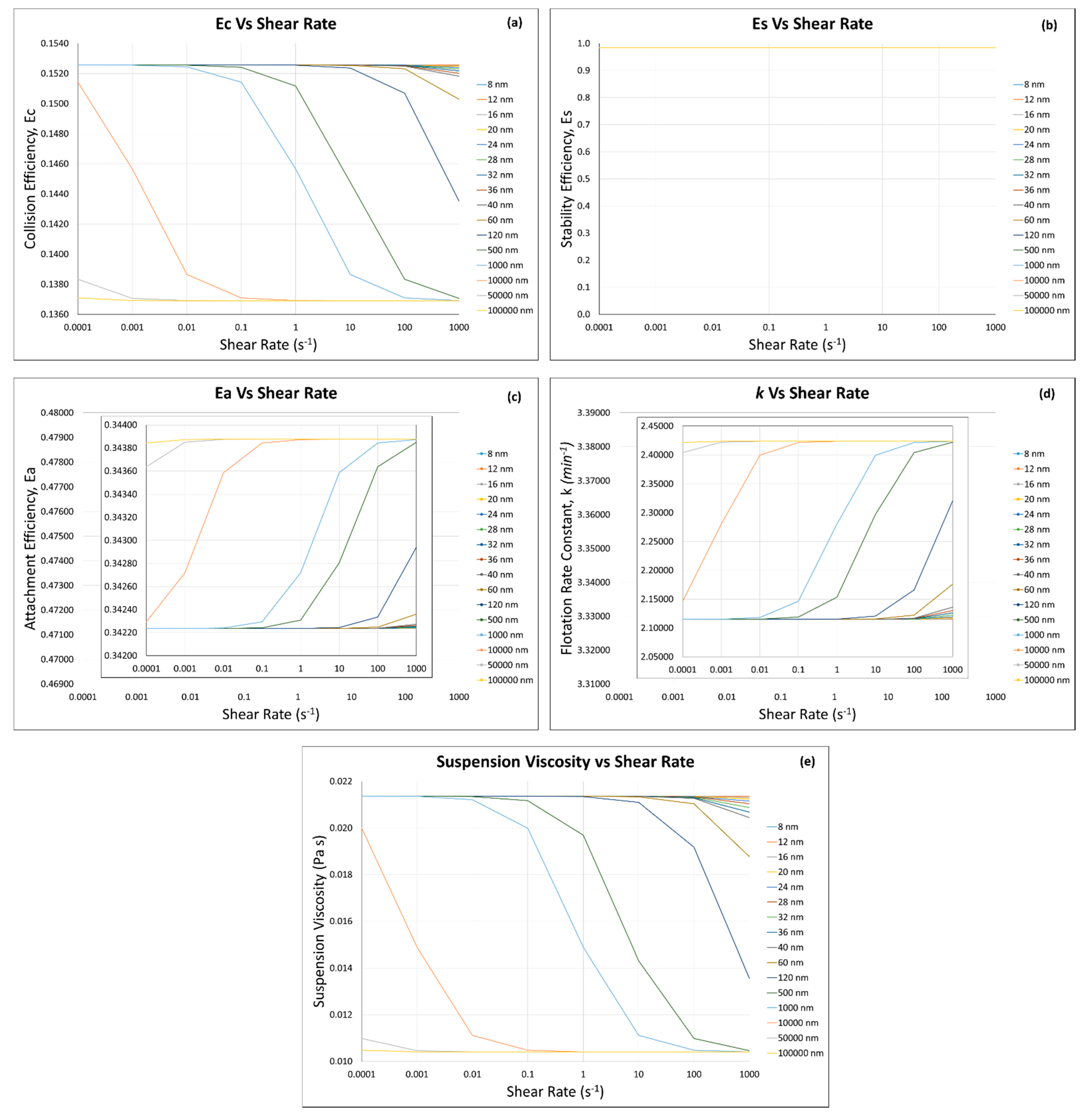
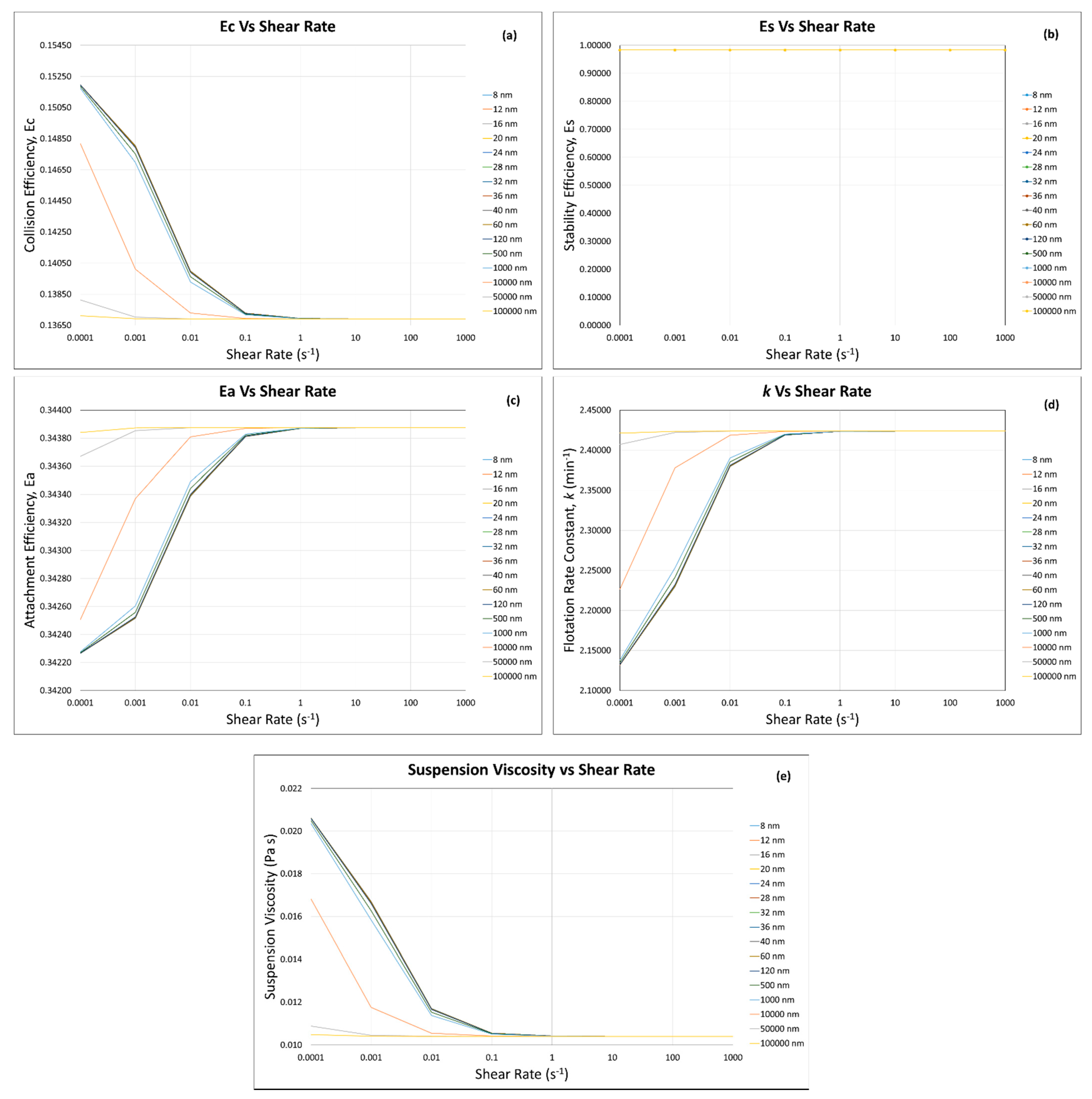
The calculations of flotation efficiencies and rate constant were carried out by using the suspension viscosity calculated by the modified Krieger and Dougherty model (Equations (19) and (24)) for the conditions mentioned in Section 3. Figure 7 and Figure 8 show that with the increase in solid fraction (i.e., $\varphi =0.1\mathrm{to}0.5$), the flotation efficiencies ($E_{\mathrm{c}}=$0.0672–0.0682 to 0.1369–0.1525 and $E_{\mathrm{a}}=$ 0.4702–0.4788 to 0.3422–0.3438) and rate constant (3.3–3.4 to 2.1–2.4 min⁻¹) changed significantly; however, $E_{\mathrm{s}}$ remained the same. The collision efficiency $\left(E_{\mathrm{c}}\right)$ increases with the decrease in ultra-fine/fine particle size (i.e., 100,000 to 8 nm) at both solid fractions (i.e., $\varphi =0.1$, Figure 7a and $0.5$, Figure 8a). This can be explained due to the fact that with the decrease in fine/ultra-fine particles (i.e., 100,000 to 8 nm), the suspension viscosity increases (from 0.00123 to 0.00128 Pa s for $\varphi =0.1$, and from 0.01047 to 0.02136 Pa s for $\varphi =0.5$) (Figure 7e and Figure 8e), and as explained earlier, the increase in suspension viscosity decreases the Stokes number (Equation (6)), which in turn increases the maximum collision angle (${\theta }_{\mathrm{t}}$) (Equation (4)). As shown in Figure 2, a higher ${\theta }_{\mathrm{t}}$ means a higher collision probability between particle and bubble.

At the low solid fraction (i.e., $\varphi =0.1$, Figure 7a), the effect of shear rate on collision efficiency $\left(E_{\mathrm{c}}\right)$ was quite dominant on the fine/ultra-fine particle size between 8 and 1000 nm, which was attributed to an increase in the hydrodynamic contributions. At the higher solid fraction (i.e., $\varphi =0.5$, Figure 8a), the effect of shear rate on $E_{\mathrm{c}}$ was dominant on intermediate ultra-fine/fine particle sizes (i.e., 60 nm–10 µm), because with increasing shear rate the hydrodynamic forces were more dominant as compared with the thermal diffusion, while above 10 µm and below 60 nm, the effect of shear rate was less dominant on the collision efficiency, because the thermal diffusion was more dominant than the hydrodynamic forces.

The stability efficiency varies with the change in turbulence dissipation energy $\left(\epsilon \right)$, particle diameter $\left(d_{\mathrm{p}}\right)$, and bubble diameter $\left(d_{\mathrm{b}}\right)$, as shown in Equation (16), which does not take into account the suspension viscosity, although the presence of fine/ultra-fine particles affected the suspension viscosity (Figure 7e and Figure 8e). All these parameters in Equation (16) remained constant in the model calculations discussed in this section, therefore stability efficiency remained unchanged ($E_{\mathrm{s}}$, Figure 7b and Figure 8b).

The attachment efficiency (Figure 7c and Figure 8c) at both solid fractions ($\varphi =0.1$ and $0.5$) decreases with the decrease in fine/ultra-fine particle size since the increased suspension viscosity at higher fine/ultra-fine particle sizes causes decrease in the attachment efficiency. Schubert (2008) [81] argued that a low pulp viscosity causes a reduction in turbulence damping, which increases the probability of particle/bubble attachment.

As seen in Figure 7e and Figure 8e, the increase in fine/ultra-fine particle size (10,000 to 100,000 nm or 10 to 100 µm) shows low suspension viscosity values (around 0.00123 Pa s for $\varphi =0.1$ and 0.01047 Pa s for $\varphi =0.5$) as compared with the smallest ultra-fine particle (8 nm), which shows slightly higher suspension viscosity values (around 0.00128 Pa s for $\varphi =0.1$ and 0.02136 Pa s for $\varphi =0.5$), and this change correlates with slightly higher $E_{\mathrm{a}}$ values (around 0.478 for $\varphi =0.1$ and 0.343 for $\varphi =0.5$) as compared with the smallest ultra-fine particle (8 nm), with $E_a$ values around 0.470 for $\varphi =0.1$ and 0.342 for $\varphi =0.5$. It was also observed in Figure 7c and Figure 8c that with the increase in solid fraction ($\varphi =0.1$ to $0.5$), $E_{\mathrm{a}}$ magnitude decreased; for example, at $\varphi =0.1$, $E_{\mathrm{a}}=0.4788$ and at $\varphi =0.5$, $E_{\mathrm{a}}=0.343$ for 100,000 nm (or 100 µm) at shear rate of 0.0001. This can be explained by the fact that at higher solid fraction, the increase in suspension viscosity (Figure 7e and Figure 8e) decreases the particle settling velocity $\left(v_{\mathrm{p}}=\frac{g{d}_{\mathrm{p}}{}^2\left({\rho }_{\mathrm{p}}-{\rho }_{\mathrm{f}}\right)}{18\mu }\right)$ and the maximum adhesion angle (Equation (8)), thus decreasing the attachment efficiency (Equation (7)).

Similar to the collision efficiency $\left(E_{\mathrm{c}}\right)$, the effect of shear rate on $E_{\mathrm{a}}$ was dominant at lower solid fraction ($\varphi =0.1$, Figure 7c) in the fine/ultra-fine to intermediate particle sizes (i.e., 8 nm–1 µm), as $E_{\mathrm{a}}$ increased from 0.470 to 0.477 for 8 nm ultra-fine particle, with an increase in shear rate from 1 to 1000 s⁻¹ (Figure 7c). Similarly, $E_{\mathrm{a}}$ increased from 0.475 to 0.488 for 1000 nm ultra-fine particle, with an increase in shear rate from 0.0001 to 0.01 s⁻¹ (Figure 7c). On the other hand, at the higher solid fraction ($\varphi =0.5$ Figure 8c), the effect of shear rate on $E_{\mathrm{a}}$ was also dominant in the intermediate fine/ultra-fine particle sizes but in a different range (i.e., 120 nm–10 µm) from $\varphi =0.1$ (Figure 7c), as $E_{\mathrm{a}}$ increased from 0.3422 to 0.3429 for 120 nm particles, with an increase in shear rate from 10 to 1000 s⁻¹. $E_{\mathrm{a}}$ also increased from 0.3422 to 0.3438 (Figure 8c) for 10 µm particles, with an increase in shear rate from 0.0001 to 0.01 s⁻¹. The dominancy of shear rate affecting $E_{\mathrm{a}}$ was observed because the hydrodynamic forces were more dominant as compared with the thermal diffusion with increasing shear rate.

The slight decrease in flotation rate constant (k) was observed with the decrease in fine/ultra-fine particle sizes at both solid fractions (i.e., $\varphi =0.1$ and $0.5$, Figure 7d and Figure 8d). For example, at the low solid fraction $\varphi =0.1$, the flotation rate constant slightly decreased from 3.37 to 3.34 min⁻¹ with the decrease in the presented particle size from 100 µm to 8 nm at a shear rate of 100 s⁻¹ (Figure 7d). Similarly, at the higher solid fraction $\varphi =0.5$ (Figure 8d), the flotation rate constant decreased from 2.42 to 2.11 min⁻¹ with the decrease in particle size from 100 µm to 8 nm at a shear rate of ≤100 s⁻¹. As stated earlier and discussed in this article and the literature, the presence of fine/ultra-fine particles has deleterious effects on the flotation rate constant/flotation performance [17,18]. Farrokhpay et al. (2016) [25] reported the copper ore flotation rate constant of 0.68 s⁻¹ (40.2 min⁻¹) in the presence of 10 wt.% kaolinite or illite, and 0.60 s⁻¹ (36 min⁻¹) in the presence of 10 wt.% montmorillonite, as compared with the copper ore flotation rate constant of 0.70 s⁻¹ (42 min⁻¹) in the absence of clay minerals. They also increased the content of fine/ultra-fine clay mineral particles as 30 wt.% kaolinite, 30 wt.% illite, or 15 wt.% montmorillonite and found further decrease in flotation rate constant to 0.51, 0.49, and 0.33 s⁻¹, respectively.

It can also be seen that with the decrease in fine/ultra-fine particle size, the suspension viscosity increases at both solid fractions $\varphi =0.1$ and $0.5$ (Figure 7e and Figure 8e); however, this increase is greater at higher solid fraction $\varphi =0.5$. For example, at $\varphi =0.1$ (Figure 7e), $\eta =0.00123$ Pa s for particle size of 100 µm, while $\eta =0.00125$ Pa s for particle size of 8 nm at a shear rate of 100 s⁻¹. At $\varphi =0.5$ (Figure 8e), $\eta =0.0104$ Pa s for particle size of 100 µm, while $\eta =0.0212$ Pa s for particle size of 8 nm at a shear rate of 100 s⁻¹. This increase in the suspension viscosity causes decrease in the flotation rate constant. For example, at $\varphi =0.1$, $k$ decreased very slightly from 3.37 to 3.34 s⁻¹ with the decrease in particle size from 100 µm to 8 nm, at a shear rate of 100 s⁻¹, while at $\varphi =0.5$, $k$ noticeably decreased from 2.42 to 2.12 s⁻¹ with the decrease in particle size from 100 µm to 8 nm, at a shear rate of 100 s⁻¹. Basnayaka et al., 2017 [33] reported that the suspension viscosity increased from 0.0018 to 0.0035 Pa s by the addition of 10 wt.% kaolin at pH 7, a shear rate of 100 s⁻¹, and a polyacrylate depressant concentration of 0 and 200 g/t, respectively. This increase in viscosity caused decrease in the flotation rate constant of the gold-bearing pyrite ore from 13.71 to 3.37 s⁻¹ (822.6 to 202.2 min⁻¹).

As seen in Figure 7a and Figure 8a, at both solid fraction $\varphi =0.1$ and $0.5$, the collision efficiency ($E_{\mathrm{c}}$) increases from 0.0672 to 0.0682 (1.49% increase) for $\varphi =0.1$, and from 0.1370 to 0.1525 (11.31% increase) for $\varphi =0.5$ with the decrease in fine/ultra-fine particle size (100 µm to 8 nm). On the other hand, as seen in Figure 7c and Figure 8c, there is a decrease in the attachment efficiency ($E_{\mathrm{a}}$) from 0.4788 to 0.4702 (1.8% decrease) for $\varphi =0.1$, and from 0.3438 to 0.3422 (0.47% decrease) for $\varphi =0.5$, with the decrease in the fine/ultra-fine particle size (100 µm to 8 nm). As shown in Figure 7d and Figure 8d, the flotation rate constant ($k$) also decreases from 3.377 to 3.319 (1.72% decrease) for $\varphi =0.1$, and from 2.421 to 2.114 (12.68% decrease) for $\varphi =0.5,$ with the decrease in fine/ultra-fine particle size (100 µm to 8 nm). It can be clearly seen that the attachment efficiency has direct influence on the flotation rate constant, and this can be explained by the magnitude of $E_{\mathrm{a}}$, which is greater than the $E_{\mathrm{c}}$ and thus has more impact on the overall $k$.

3.4.2. Incorporation of Our Predictive Model—Hard Sphere and Interacting Colloidal Particle Suspensions

Homogeneous Case—Same Particles with the Same Sizes

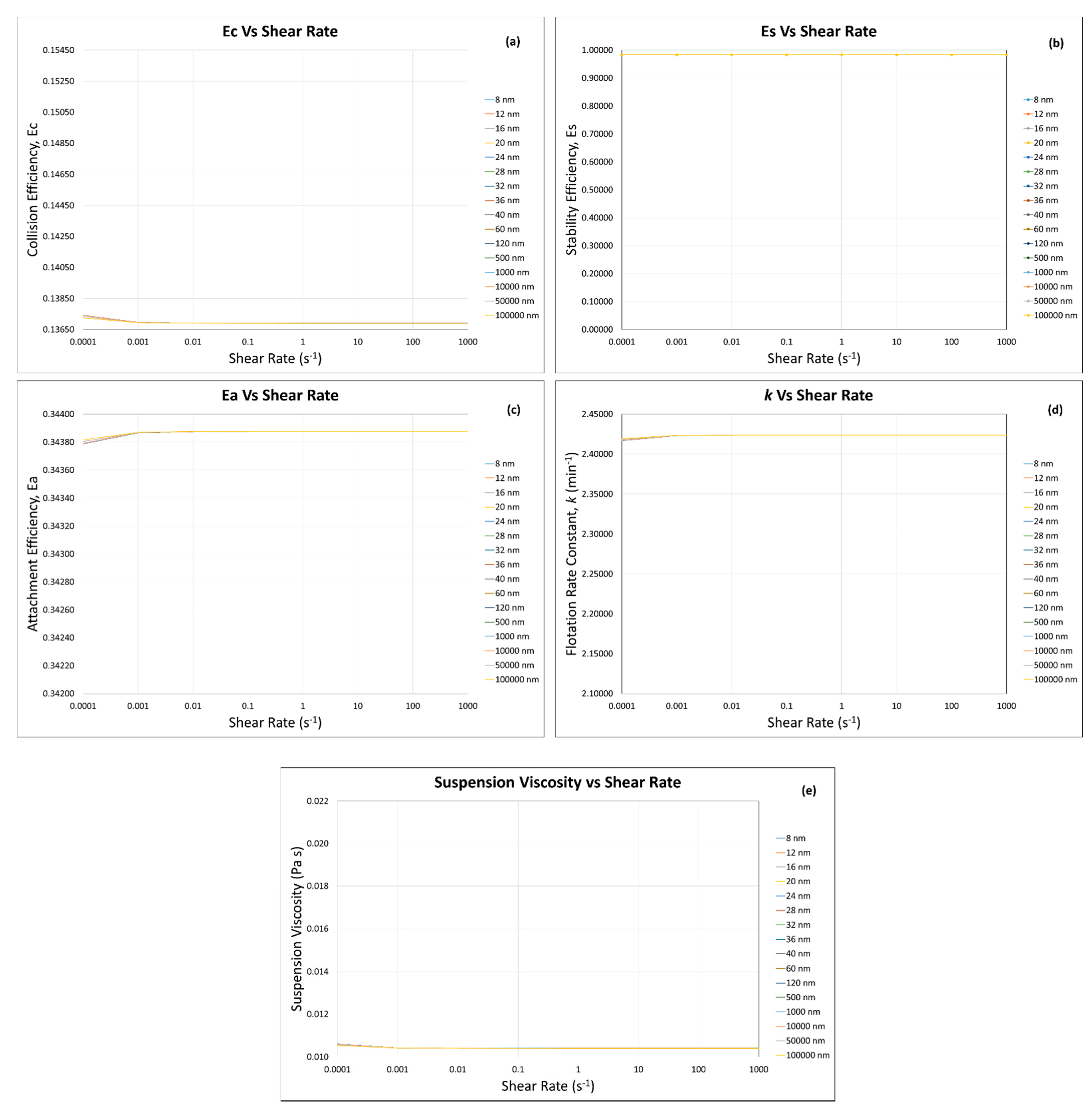
The calculations of flotation efficiencies and rate constant were carried out by using the suspension viscosity calculated by our predictive model (Equations (19), (25), (27) and (33)) for the same quartz particles with the same sizes (Figure 9 and Figure 10) under the following conditions: pH = 10, zeta potential value = −50 mV, and salt concentration and type = 1 × 10⁻² M KNO₃, as well as the other conditions mentioned in Section 3. The flotation efficiencies and rate constant (Figure 9 and Figure 10) almost follow the same general trends as of the modified Krieger and Dougherty model coupling (Figure 7 and Figure 8), with a slight change in their absolute values (increase in $E_{\mathrm{c}}$ and decrease in $E_{\mathrm{a}}$ and $k$, but $E_{\mathrm{s}}$ remained same). For instance, at solid fraction $\varphi =0.1$, with the decrease in fine/ultra-fine particle size (100 μm to 8 nm) $E_{\mathrm{c}}$ increased from 0.06729 to 0.06830 (1.5% increase), $E_{\mathrm{a}}$ decreased from 0.4788 to 0.4702 (1.8% decrease), $k$ decreased from 3.3775 to 3.3196 min⁻¹ (1.71% decrease), and $E_{\mathrm{s}}$ remained unchanged. As our predictive model incorporates the total potential energies calculated by using the DLVO theory (Table 2), it leads to this additional increase in the magnitude of flotation efficiencies and rate constant. The DLVO calculations were made using Equations (25)–(30) for the conditions stated in the beginning of this section. At a lower solid fraction ($\varphi =0.1$), with the increase in particle size (8 nm to 100 μm), the interparticle distance (calculated from Equation (26)) increased; therefore, the total potential energies (van der Walls and electric double-layer) decreased, resulting in a decrease in the suspension viscosity from 0.001285 to 0001232 Pa s (4.12% decrease). Otsuki and Hayagan (2020) [73] studied the surface properties of hematite and gangue minerals and their mixtures with the bentonite binder to understand and properly control their surface properties for pelletization of fine hematite ores. They calculated the total potential between quartz–quartz particles and reported the similar trend of decrease in total potential with the increase in interparticle distance, as we reported here. As shown in Table 2, at higher solid fractions ($\varphi >0.3)$, the DLVO calculations become inapplicable because the calculated viscosity values from Equation (33) are too high; thus, the following flotation efficiencies and rate constant calculations were made at $\varphi$ ≤ 0.3, and their results are shown in Figure 9 ($\varphi =$ 0.1) and Figure 10 ($\varphi =$ 0.3) in this section. At the higher solid fraction ($\varphi =$ 0.3), the interparticle distance decreases (e.g., for 8 nm and 80 μm particles, interparticle distance decreased from 5.86 to 1.61 nm, with the increase in solid fraction from $\varphi =0.1$ to $\varphi =0.3$), and thus the van der Waals potential energy $V_A$ decreased from −0.472 × 10⁻²¹ to −1.71 × 10⁻²¹ K_BT, while electrical double-layer potential $V_R$ increased from 5.46 × 10⁻²¹ to 22.1 × 10⁻²¹ K_BT, and the total potential energy $V_T$ increased from 4.99 × 10⁻²¹ to 20.4 × 10⁻²¹ K_BT with the increase in solid fraction from $\varphi =0.1$ to $\varphi =0.3$). This resulted in higher values of the suspension viscosity (i.e., 0.002729–0.003314 Pa s for $\varphi =$ 0.3, as compared to 0.00123–0.00128 Pa s for $\varphi =$ 0.1) (Figure 9e and Figure 10e). This indicates that electrostatic repulsive interaction could be responsible for the increase in suspension viscosity, as Sakairi et al. (2005) [84] reported that electrostatic repulsion was the cause of increase in their montmorillonite suspension yield stress. The higher suspension viscosity leads to the change in flotation efficiencies (Figure 10a,c) and rate constant (Figure 10d). For example, $E_{\mathrm{c}}$ increased from 0.06729–006830 for $\varphi =$ 0.1 to 0.09849–0.09146 for $\varphi =$ 0.3, $E_{\mathrm{a}}$ decreased from 0.4788–0.4702 for $\varphi =$ 0.1 to 0.3768–0.3658 for $\varphi =$ 0.3, $k$ decreased from 3.377–3.319 min⁻¹ for $\varphi =$ 0.1 to 2.720–2.7163 min⁻¹ for $\varphi =$ 0.3, and $E_{\mathrm{s}}$ remained constant.

The decrease in flotation rate constant with the decrease in fine/ultra-fine particle size can be due to the deleterious effect of fine/ultra-fine particles, which agrees with the literature. Basnayaka et al., 2017 [33] reported that the suspension viscosity increased from 0.0018 to 0.0035 Pa s by the addition of 10 wt.% (3.77 vol.%) kaolin at pH 7, a shear rate of 100 s⁻¹, and a polyacrylate depressant concentration of 0 and 200 g/t, respectively. This increase in viscosity caused a decrease in the flotation rate constant of the gold-bearing pyrite ore from 13.71 to 3.37 s⁻¹ (822.6 to 202.2 min⁻¹, 75.4% decrease). The presence of bentonite under the same conditions reduced the flotation rate constant to 4.14 s⁻¹ (248.4 min⁻¹, 69.8% decrease). Using their suspension viscosity values for the case of kaolin, in our predictive model, the flotation rate constant clearly indicates its decrease from 2.982 to 2.703 min⁻¹ (9.36% decrease), although the literature system and our system are different. Our predictive model calculations were made on the quartz particles.

Zhang and Peng (2015) [14] reported a decrease in copper recovery from 80 to 60% in the absence and the presence of 15 wt.% bentonite, which caused an increase in the apparent viscosity from 0.0018 to 0.0079 Pa s. Using their suspension viscosity values in our predictive model, the flotation rate constant decreases from 2.982 to 2.514 min⁻¹ (15.69% decrease). The possible reasons for such decreases in flotation rate constant were reported as the occurrence of slime coating or physical adsorption of clay mineral particles onto the copper-containing mineral surface [28].

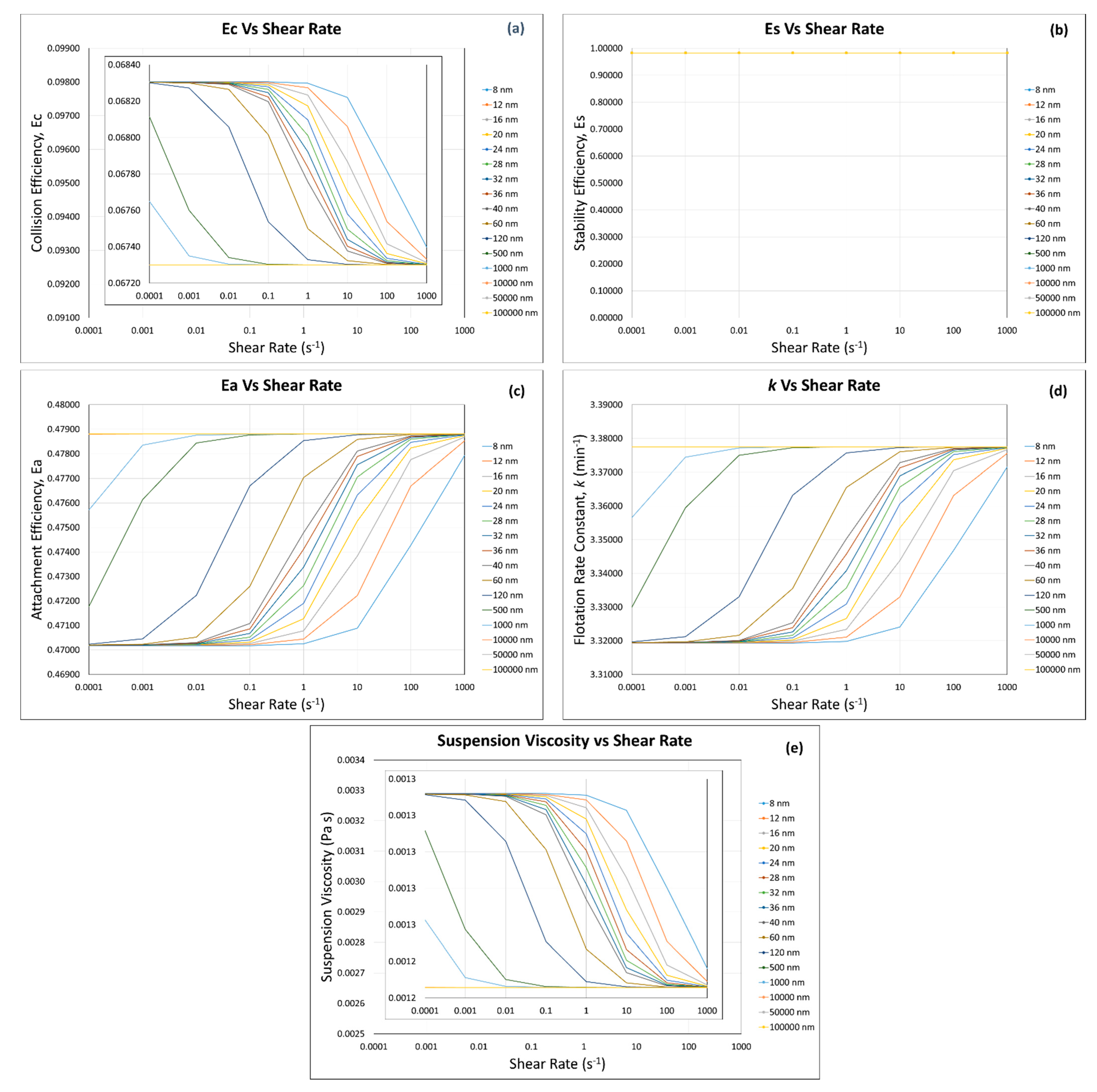
Homogeneous Case—Same Particle with Different Particle Sizes

The calculations for flotation efficiencies and rate constant were carried out by using the predictive model for the same quartz particles with different particle sizes (Figure 11, Figure 12, Figure 13 and Figure 14) for the conditions mentioned in Section 3 and the previous section “Homogeneous Case—Same Particles with the Same Sizes”. It can be seen in Figure 11a that at low solid fraction ($\varphi =0.1$), when the percentage of coarse particle (i.e., 80 µm) was 10 vol.% as compared with the fine/ultra-fine particles (i.e., 90 vol.%), there is a slight decrease in collision efficiency (0.06730 to 0.06729, 1.4% decrease) with the increase in fine/ultra-fine particle size (8 nm to 100 μm) with increasing shear rate (0.0001 to 100 s⁻¹). However, it can be seen that the decrease in collision efficiency took place up to the shear rate of 0.01 s⁻¹, and above 0.01 s⁻¹ shear rate, the collision efficiency became almost constant. This can be explained by the effect of suspension viscosity (Figure 11e), as below the shear rate of 0.01 s⁻¹, the suspension viscosity very slightly increases (from 0.00123289 to 0.00123295 Pa s with the decrease in fine/ultra-fine particle size of 100 μm to 8 nm). The increase in suspension viscosity decreases the Stokes number (Equation (6)), which in turn increases the maximum collision angle (${\theta }_{\mathrm{t}}$) (Equation (4)). As shown in Figure 2, a higher ${\theta }_t$ means higher collision probability between a particle and a bubble.

Figure 11c shows a very limited decrease in attachment efficiency from 0.4788 to 0.4787 (0.02% decrease) with the decrease in fine/ultra-fine particles (100 µm to 8 nm). This can be explained by the fact that the decrease in fine/ultra-fine particles size increased the suspension viscosity. The increased suspension viscosity decreases the bubble Reynolds number (Equation (12)), which in turn increases the maximum collision angle (${\theta }_{\mathrm{t}}$) (Equation (4)), and as shown in Equation (7), a higher ${\theta }_{\mathrm{t}}$ reduces the attachment efficiency.

Figure 11d shows negligible change in flotation rate constant from 3.3775 to 3.3774 min⁻¹ (0.003% decrease) with the decrease in the fine/ultra-fine particle size (100 µm to 8 nm). This can be explained by the effect of suspension viscosity and the flotation efficiencies ($E_{\mathrm{c}}$ and $E_{\mathrm{a}}$). The decrease in fine/ultra-fine particles very slightly increased the suspension viscosity from 0.00123289 to 0.00123295 Pa s (0.005% increase), especially at low shear rates (below 0.01 s⁻¹). This degree of suspension viscosity increase caused negligible change in the flotation rate constant, from 3.3775 to 3.3774 min⁻¹ (0.003% decrease).

Secondly, although the collision efficiency increased with the decrease in fine/ultra-fine particle size and the attachment efficiency decreases with the increase in fine/ultra-fine particle size, the magnitude of these two efficiencies affected the flotation rate constant. It can be seen that the magnitude of attachment efficiency (Figure 11c) (between 0.4788 and 0.4787) is much greater than the collision efficiency (Figure 11a) (between 0.06730 and 0.06729). Thus, the attachment efficiency has more influence than the collision efficiency on flotation rate constant, which decreased with the decrease in fine/ultra-fine particles.

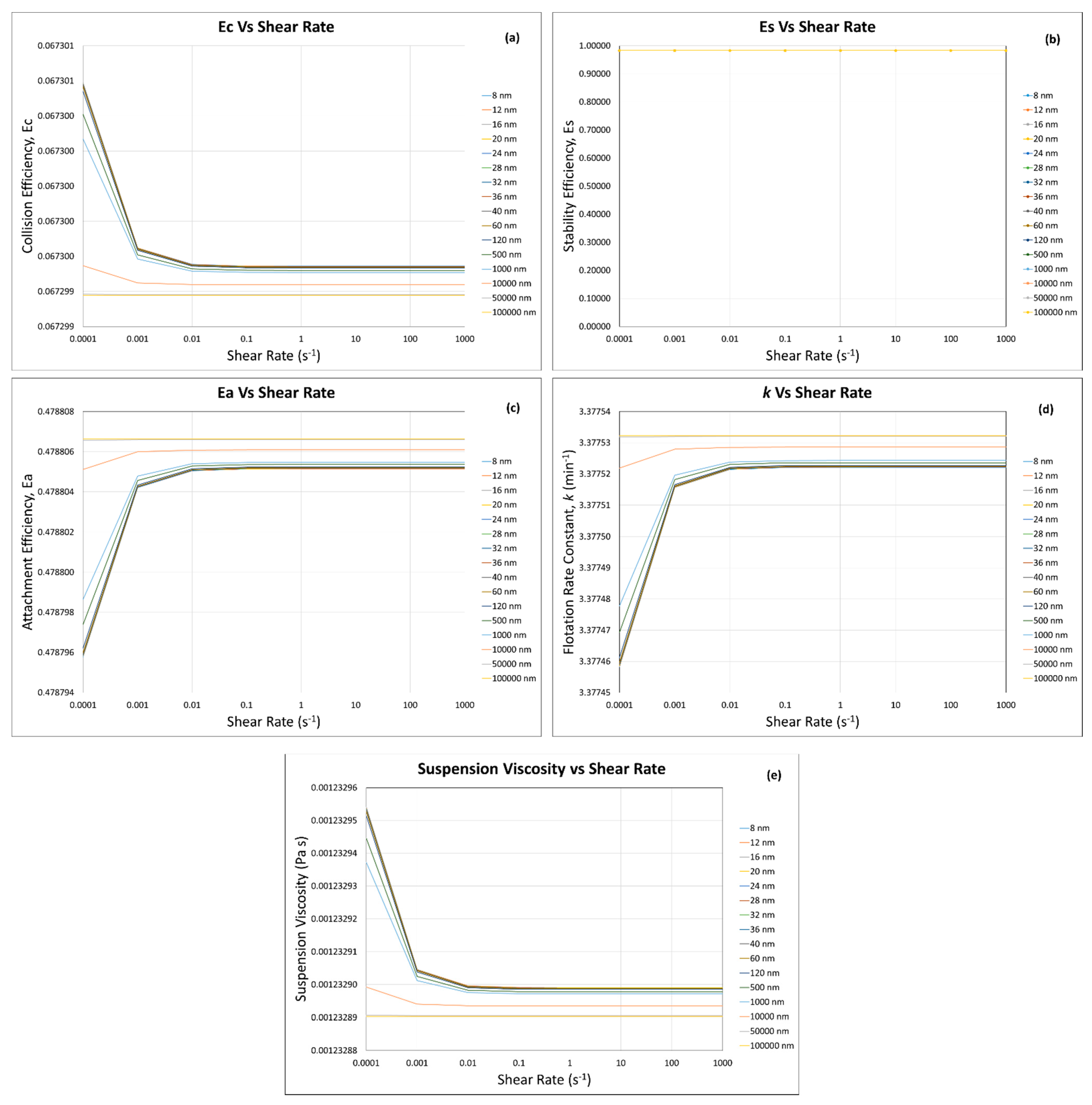
When the percentage of coarse particles (i.e., 80 µm) was 90 vol.% as compared with the ultra-fine/fine particles (i.e., 10 vol.%), there was very little change in the flotation efficiencies ($E_{\mathrm{c}}$ increased from 0.067299379 to 0.067299535, 0.00023% increase; $E_{\mathrm{a}}$ decreased from 0.478806 to 0.478805, 0.00021% decrease) and rate constant (3.377532–3.377522, 0.0003% decrease) (Figure 12a,c,d). This can be explained by the fact that at a higher concentration of coarse particles, the viscosity change was very limited (0.001232890 to 0.001232899, 0.0007% increase) (Figure 12e). Therefore, it had an almost negligible effect on the flotation efficiencies and rate constant. Wang et al. (2015) [16] reported an increase in apparent viscosity of copper–gold ore slurry from 0.00085 to 0.00095 Pa s (10.5% increase) with an increase in solid concentration from 0 to 5 wt.% of bentonite, and this change in suspension viscosity decreased the copper recovery from 90% to 88%. Contrary to this, with 15 wt.% of bentonite, the apparent viscosity of the suspension increased to 0.0023 Pa s, and the copper recovery decreased to 80%. Thus, it can be deduced that when the fine/ultra-fine particles are present in a small quantity (i.e., 10 vol.%), they have very limited influence on the flotation efficiencies and rate constant (Figure 12a,c,d), as they have almost negligible influence on the suspension viscosity (Figure 12e).

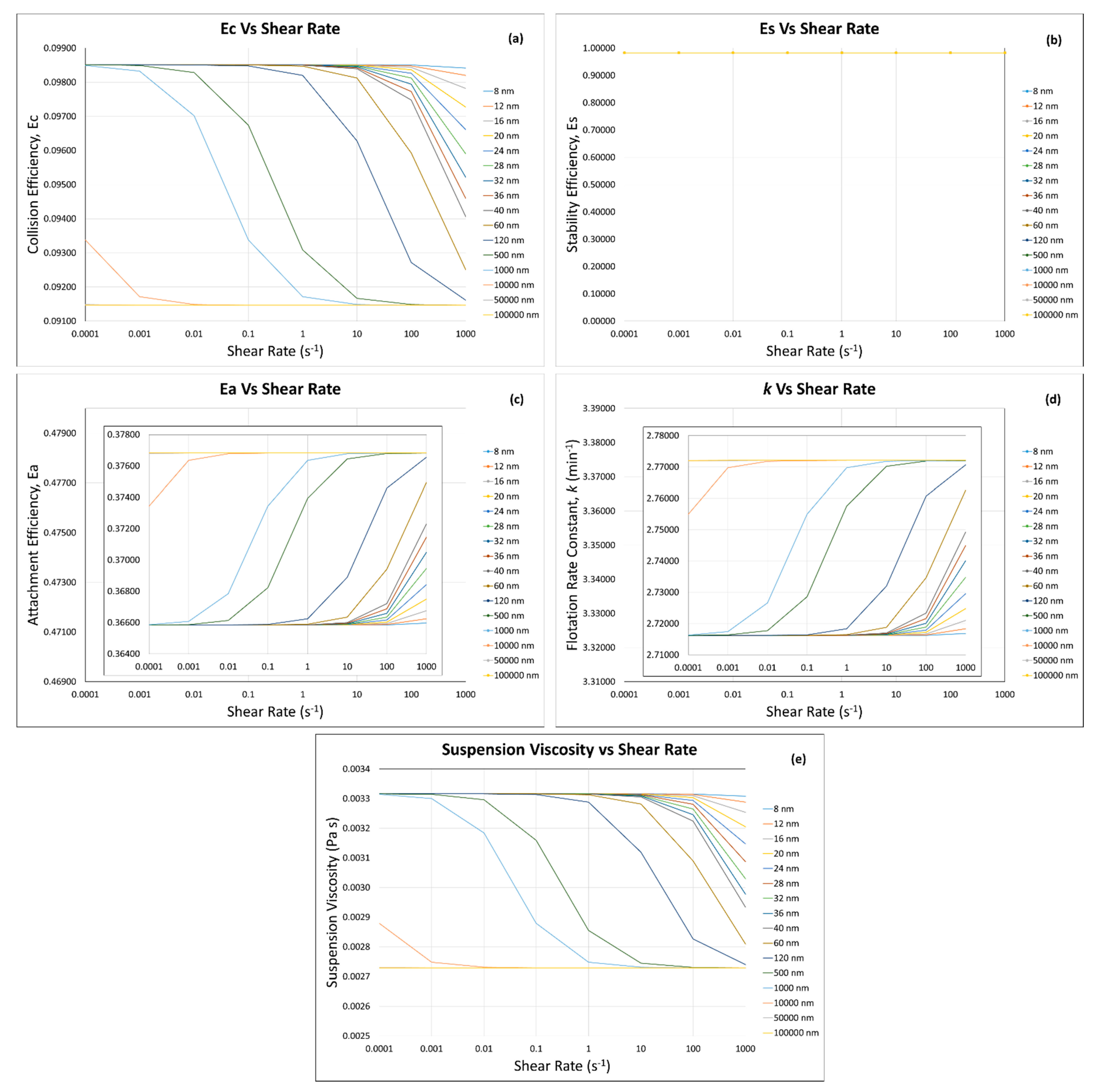
At the higher solid fraction (i.e., $\varphi =0.5$), when the percentage of coarse particle (i.e., 80 µm) was 10 vol.% as compared with the fine/ultra-fine particles (i.e., 90 vol.%), the collision efficiency (Figure 13a) showed a similar increasing trend with the decrease in fine/ultra-fine particle size as that for $\varphi =0.1$ (Figure 11a). However, its magnitude increased (0.06730 to 0.06729 for $\varphi =0.1$, and 0.1371 to 0.1518 for $\varphi =0.5$), and this increase can be explained by our calculation results showing that at higher solid fraction $\left(\varphi =0.5\right)$, the suspension viscosity increases (from 0.010410134 to 0.02049303 Pa s, 96.8% increase with the decrease in fine/ultra-fine particle size of 100 μm to 8 nm). The increase in suspension viscosity decreases the Stokes number (Equation (6)), which in turn increases the maximum collision angle (${\theta }_{\mathrm{t}}$) (Equation (4)). As shown in Figure 2, a higher ${\theta }_{\mathrm{t}}$ means a higher collision probability between a particle and a bubble.

The attachment efficiency (Figure 13c) also showed a similar decreasing trend with the decrease in fine/ultra-fine particle size as that for $\varphi =0.1$. However, its magnitude was decreased (0.4788 to 0.4787 for $\varphi =0.1$, and 0.3422 to 0.3438 for $\varphi =0.5$), and this can be explained by the fact that at higher solid fraction $\left(\varphi =0.5\right)$, the magnitude of suspension viscosity increased for $\varphi =0.5$ (0.01048 to 0.02035 Pa s) as compared with the ones for $\varphi =0.1$ (0.00123289 to 0.00123295 Pa s).

The flotation rate constant k (Figure 13d) was mainly influenced by the significant decrease in the attachment efficiency $E_{\mathrm{a}}$ and the suspension viscosity that is a function of the solid fraction (Equations (19) and (33)). Therefore, with the increase in solid fraction, k decreased from its range between 3.3775 and 3.3774 min⁻¹ at $\varphi =0.1$ to its range between 2.137 and 2.421 min⁻¹ at $\varphi =0.5$.

When the percentage of coarse particles (i.e., 80 µm) was 10 vol.% as compared with the ultra-fine/fine particles (i.e., 90 vol.%), at the higher solid fraction $\left(\varphi =0.5\right)$, the role of shear rate was clearly observed. The increase in shear rate (0.0001 to 0.01 s⁻¹) causes decrease in the suspension viscosity from 0.02035 to 0.01040 Pa s (48.9% decrease, Figure 13e). This shows that the hydrodynamic forces are dominant on the interparticle forces above 0.01 s⁻¹ shear rate, and the viscosity does not change significantly, showing that the hydrodynamic forces become fully dominant on the interparticle forces. Genovese (2012) [21] calculated a relative viscosity (${\eta }_{\mathrm{r}}$) and reported that ${\eta }_{\mathrm{r}}$ increased with solid fraction and decreased with shear rate, but he mentioned that the shear thinning effect was only noticeable at approximately $\varphi >0.25$ and at high shear rates (>100 s⁻¹) where hydrodynamic forces become more significant than interparticle forces. He further explained that the viscosity decrease in this shear-thinning region was due to the ordering of particles along the flow direction.

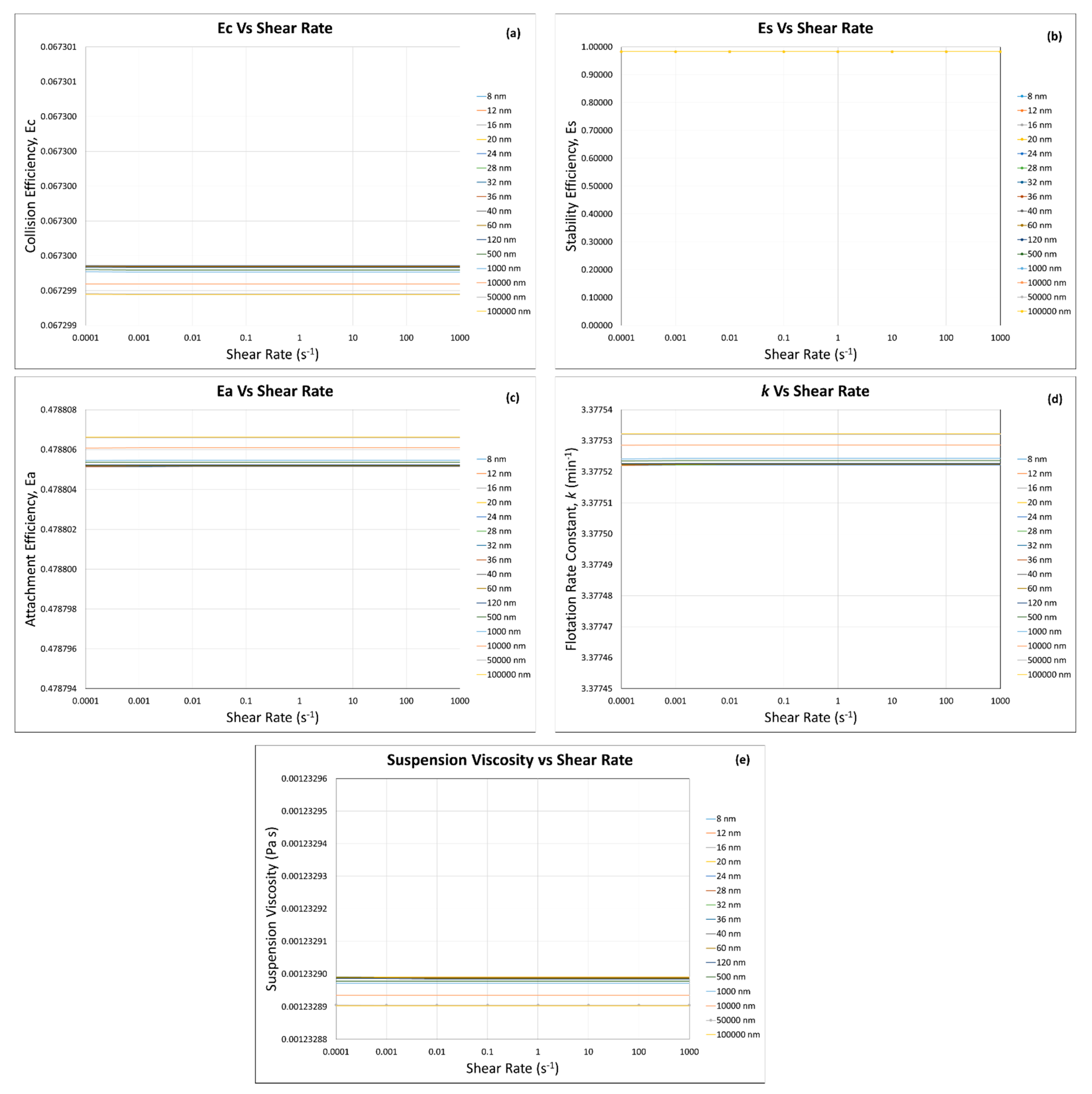
When the percentage of coarse particles (i.e., 80 µm) was 90 vol.% as compared with the fine/ultra-fine particles (i.e., 10 vol.%), at solid fraction $\left(\varphi =0.5\right)$, the suspension viscosity (Figure 14e) shows a similar behavior as that of the solid fraction $\left(\varphi =0.1\right)$ (Figure 12e). This behavior was obvious, as the coarse particles were 90% in volume, which did not allow the other 10% of fine/ultra-fine particles to change the suspension viscosity and later on the flotation efficiencies and rate constant. As the flotation efficiencies and rate constant are directly influenced by the suspension viscosity, which in this case did not change, almost negligible change was seen, as shown in Figure 14a,b,d.

4. Conclusions

Flotation of fine particles has become particularly important in recent years as advances in grinding are allowing low-grade mineral deposits to be economically exploited. The fine particles have several deleterious effects on the entire flotation process—that is, (1) their high level of entrainment, in the wake of the rising bubbles, can dilute the concentrate if the entrained particles are gangue minerals; and (2) the increase in the suspension viscosity, which has negative effect on the flotation efficiencies and rate constant. The latter effect was addressed in this work by understanding and calculating the suspension viscosity of fine/ultra-fine particles ranging from 8 nm to 100 μm and then incorporating it into the flotation kinetics model to calculate the flotation efficiencies and rate constant for a mechanical flotation size particle (i.e., 80 μm) for the first time. This coupling study started with the simplest case: flowing suspensions of inert, rigid, monomodal spherical particles (called hard spheres) at low shear rates. Then, the effect of viscosity of the colloidal particle suspensions, where interparticle forces play a significant role, on the flotation efficiencies and rate constant for a mechanical flotation size particle were studied. It was observed that coupling the flotation kinetics model and viscosity model clearly addressed the change in flotation efficiencies and rate constant as a function of suspension viscosity that can be varied with solid concentration, shear rate, and particle size. Our modelled results clearly and systematically illustrated the effect of the above-mentioned parameters on suspension viscosity and thus flotation efficiencies and rate constant at the very first time, while the previous literature provides valid discussion within limited and very specific points of interest. From our model calculations, it was found that under our calculated conditions, the magnitude and change in the attachment efficiency assigned by the change in suspension viscosity were often greater than those of the collision and stability efficiencies. Thus, the trend observed in the attachment efficiency with the change in suspension viscosity greatly influenced the flotation rate constant. With our model, for example, effects of composition of raw materials and flotation reagent for real mineral systems on flotation rate constant can be studied in the future.

References

- Venditti, R.A. A Simple Flotation De-Inking Experiment for the Recycling of Paper. J. Chem. Educ. 2004, 81, 693. [Google Scholar] [CrossRef]
- Wang, C.; Wang, H.; Fu, J.; Liu, Y. Flotation separation of waste plastics for recycling-A review. Waste Manag. 2015, 41, 28–38. [Google Scholar] [CrossRef] [PubMed]
- Zheng, Y.; Zhao, C. A study of the kinetics on induced-air flotation for oil-water separation. Sep. Sci. Technol. 1993, 28, 1233–1240. [Google Scholar] [CrossRef]
- Rubio, J.; Souza, M.; Smith, R.W. Overview of flotation as a wastewater treatment technique. Miner. Eng. 2002, 15, 139–155. [Google Scholar] [CrossRef]
- Pyke, B.; Fornasiero, D.; Ralston, J. Bubble particle heterocoagulation under turbulent conditions. J. Colloid Interface Sci. 2003, 265, 141–151. [Google Scholar] [CrossRef]
- Sajjad, M.; Otsuki, A. Correlation between Flotation and Rheology of Fine Particle Suspensions. Metals 2022, 12, 270. [Google Scholar] [CrossRef]
- Dai, Z.; Dukhin, S.; Fornasiero, D.; Ralston, J. The Inertial Hydrodynamic Interaction of Particles and Rising Bubbles with Mobile Surfaces. J. Colloid Interface Sci. 1998, 197, 275–292. [Google Scholar] [CrossRef]
- Szatkowski, M. A model of flotation selectivity. Int. J. Miner. Process. 1988, 23, 25–31. [Google Scholar] [CrossRef]
- Schulze, H.J. Physico–Chemical Elementary Processes in Flotation: An Analysis from the Point of View of Colloid Science Including Process Engineering Considerations; Elsevier: Amsterdam, The Netherlands, 1984. [Google Scholar]
- Dukhin, S.S.; Kretzschmar, G.; Miller, R. Dynamics of Adsorption at Liquid Interfaces, 1st ed.; Elsevier Science: Amsterdam, The Netherlands, 1995. [Google Scholar]
- Duan, J.; Fornasiero, D.; Ralston, J. Calculation of the flotation rate constant of chalcopyrite particles in an ore. Int. J. Miner. Process. 2003, 72, 227–237. [Google Scholar] [CrossRef]
- Jameson, G.J.; Nam, S.; Young, M.M. Physical Factors Affecting Recovery Rates in Flotation. Miner. Sci. Eng. 1997, 9, 103–118. [Google Scholar]
- Radoev, B.P.; Alexandrova, L.; Tchaljovska, S. On the kinetics of froth flotation. Int. J. Miner. Process. 1990, 28, 127–138. [Google Scholar] [CrossRef]
- Zhang, M.; Peng, Y. Effect of clay minerals on pulp rheology and the flotation of copper and gold minerals. Miner. Eng. 2015, 70, 8–13. [Google Scholar] [CrossRef]
- Xu, D.; Ametov, I.; Grano, S.R. Quantifying rheological and fine particle attachment contributions to coarse particle recovery in flotation. Miner. Eng. 2012, 39, 89–98. [Google Scholar] [CrossRef]
- Wang, Y.; Peng, Y.; Nicholson, T.M.; Lauten, R.A. The different effects of bentonite and kaolin on copper flotation. Appl. Clay Sci. 2015, 114, 48–52. [Google Scholar] [CrossRef]
- Farrokhpay, S.; Ndlovu, B.N.; Bradshaw, D.J. Behavior of talc and mica in copper ore flotation. Appl. Clay Sci. 2018, 160, 270–275. [Google Scholar] [CrossRef]
- Chen, X.; Hadde, E.; Liu, S.; Peng, Y. The effect of amorphous silica on pulp rheology and copper flotation. Miner. Eng. 2017, 113, 41–46. [Google Scholar] [CrossRef]
- Zhang, M.; Peng, Y.; Xu, N. The effect of sea water on copper and gold flotation in the presence of bentonite. Miner. Eng. 2015, 77, 93–98. [Google Scholar] [CrossRef]
- Cruz, N.; Peng, Y.; Wightman, E.M.; Xu, N. The interaction of clay minerals with gypsum and its effects on copper–gold flotation. Miner. Eng. 2015, 77, 121–130. [Google Scholar] [CrossRef]
- Genovese, D.B. Shear rheology of hard-sphere, dispersed, and aggregated suspensions, and filler-matrix composites. Adv. Colloid Interface Sci. 2012, 171, 1–16. [Google Scholar] [CrossRef]
- Ogawa, A.; Yamada, H.; Matsuda, S.; Okajima, K. Viscosity equation for concentrated suspensions of charged colloidal particles. J. Rheol. 1997, 41, 769–785. [Google Scholar] [CrossRef]
- Zhang, W. Evaluation of effect of viscosity changes on bubble size in a mechanical flotation cell. Trans. Nonferrous Met. Soc. China 2014, 24, 2964–2968. [Google Scholar] [CrossRef]
- Farrokhpay, S.; Ametov, I.; Grano, S.R. Improving the recovery of low grade coarse composite particles in porphyry copper ores. Adv. Powder Technol. 2011, 22, 464–470. [Google Scholar] [CrossRef]
- Farrokhpay, S.; Bulelwa, N.; Dee, B. Behaviour of swelling clays versus non-swelling clays in flotation. Miner. Eng. 2016, 96, 59–66. [Google Scholar] [CrossRef]
- Shabalala, N.Z.; Harris, M.C.; Leal-Filho, L.D.S.; Deglon, D.A. Effect of slurry rheology on gas dispersion in a pilot-scale mechanical flotation cell. Miner. Eng. 2011, 24, 1448–1453. [Google Scholar] [CrossRef]
- Becker, M.; Yorath, G.; Ndlovu, B.; Harris, M.C.; Deglon, D.A.; Franzidis, J.P. A rheological investigation of the behaviour of two Southern African platinum ores. Miner. Eng. 2013, 49, 92–97. [Google Scholar] [CrossRef]
- Forbes, E.; Davey, K.J.; Smith, L. Decoupling rheology and slime coatings effect on the natural floatability of chalcopyrite in a clay-rich flotation pulp. Miner. Eng. 2014, 56, 136–144. [Google Scholar] [CrossRef]
- Bakker, C.W.; Meyer, C.J.; Deglon, D.A. Numerical modelling of non-Newtonian slurry in a mechanical flotation cell. Miner. Eng. 2009, 22, 944–950. [Google Scholar] [CrossRef]
- Otsuki, A.; Chen, Y.; Zhao, Y. Characterisation and Beneficiation of Complex Ores for Sustainable Use of Mineral Resources: Refractory Gold Ore Beneficiation as an Example. Int. J. Soc. Mater. Eng. Resour. 2014, 20, 126–135. [Google Scholar] [CrossRef] [Green Version]
- Derjaguin, B.V. Theory of Stability of Colloids and Thin Films; English Translation; Plenum: New York, NY, USA, 1989. (In Russian) [Google Scholar]
- Verwey, E.J.W. Theory of the Stability of Lyophobic Colloids; Elsevier Publishing Company Inc.: Amsterdam, The Netherlands, 1948. [Google Scholar]
- Basnayaka, L.; Subasinghe, N.; Albijanic, B. Influence of clays on the slurry rheology and flotation of a pyritic gold ore. Appl. Clay Sci. 2017, 136, 230–238. [Google Scholar] [CrossRef]
- Levich, V. Physicochemical Hydrodynamics; Prentice-Hall: Englewood Cliffs, NJ, USA, 1962. [Google Scholar]
- van de Ven, T. Colloidal Hydrodynamics; Academic Press: London, UK, 1989. [Google Scholar]
- Churaev, N.V.; Derjaguin, B.V.; Muller, V. Surface Forces; Springer: New York, NY, USA, 1987. [Google Scholar]
- Edwards, D.A.; Brenner, H.; Wasan, D.T. Interfacial Transport Processes and Rheology; Butterworth-Heinemann: London, UK, 1991. [Google Scholar]
- Ivanov, I.; Dimitrov, D. Thin Liquid Films; Dekker: New York, NY, USA, 1988. [Google Scholar]
- Derjaguin, B.V.; Churaev, N.V. Wetting Films; Nauka: Moscow, Russia, 1984. [Google Scholar]
- Overbeek, J.T.G. Recent developments in the understanding of colloid stability. J. Colloid Interface Sci. 1977, 58, 408–422. [Google Scholar] [CrossRef]
- Kihira, H.; Matijevic, E. An assessment of heterocoagulation theories. Adv. Colloid Interface Sci. 1992, 42, 1–31. [Google Scholar] [CrossRef]
- Kouachi, S.; Hassas, B.V.; Hassanzadeh, A.; Çelik, M.S.; Bouhengue, M. Effect of negative inertial forces on bubble-particle collision via implementation of Schulze collision efficiency in general flotation rate constant equation. Colloids Surf. A Physicochem. Eng. Asp. 2017, 517, 72–83. [Google Scholar] [CrossRef]
- Hewitt, D.J.; Fornasiero, D.; Ralston, J. Bubble–particle attachment. J. Chem. Soc. Faraday Trans. 1995, 91, 1997–2001. [Google Scholar] [CrossRef]
- Dai, Z.; Fornasiero, D.; Ralston, J. Particle–Bubble Attachment in Mineral Flotation. J. Colloid Interface Sci. 1999, 217, 70–76. [Google Scholar] [CrossRef] [PubMed]
- Dobby, G.S.; Finch, J.A. Particle size dependence in flotation derived from a fundamental model of the capture process. Int. J. Miner. Process. 1987, 21, 241–260. [Google Scholar] [CrossRef]
- Crawford, R.; Ralston, J. The influence of particle size and contact angle in mineral flotation. Int. J. Miner. Process. 1988, 23, 1–24. [Google Scholar] [CrossRef]
- van Nguyen, A.; Ralston, J.; Schulze, H.J. On modelling of bubble-particle attachment probability in flotation. Int. J. Miner. Process. 1998, 53, 225–249. [Google Scholar] [CrossRef]
- Ahmed, N.; Jameson, G.J. The Effect of Bubble Size on the Rate of Flotation of Fine Particles. Int. J. Miner. Process. 1985, 14, 195–215. [Google Scholar] [CrossRef]
- Dai, Z.; Fornasiero, D.; Ralston, J. Particle–bubble collision models—A review. Adv. Colloid Interface Sci. 2000, 85, 231–256. [Google Scholar] [CrossRef]
- Phan, C.M.; van Nguyen, A.; Miller, J.D.; Evans, G.M.; Jameson, G.J. Investigations of bubble–particle interactions. Int. J. Miner. Process. 2003, 72, 239–254. [Google Scholar] [CrossRef]
- Sutherland, K. Physical Chemistry of Flotation. XI. Kinetics of the flotation process. J. Phys. Colloid Chem. 1948, 52, 394–425. [Google Scholar] [CrossRef] [PubMed]
- Dukhin, S.S. Role of inertial forces in flotation of small particles. Colloid J. USSR 1982, 44, 388–397. [Google Scholar]
- Ralston, J.; Fornasiero, D.; Hayes, R. Bubble–particle attachment and detachment in flotation. Int. J. Miner. Process. 1999, 56, 133–164. [Google Scholar] [CrossRef]
- Ralston, J.; Dukhin, S.S.; Mishchuk, N.A. Inertial hydrodynamic particle–bubble interaction in flotation. Int. J. Miner. Process. 1999, 56, 207–256. [Google Scholar] [CrossRef]
- van Nguyen, A.; Schulze, H.J.; Ralston, J. Elementary steps in particle—bubble attachment. Int. J. Miner. Process. 1997, 51, 183–195. [Google Scholar] [CrossRef]
- Hassas, B.V.; Kouachi, S.; Eskanlou, A.; Bouhenguel, M.; Çelik, M.S.; Miller, J.D. The significance of positive and negative inertial forces in Particle-Bubble interaction and their role in the general flotation kinetics model. Miner. Eng. 2021, 170, 107006. [Google Scholar] [CrossRef]
- Schulze, H.J. Hydrodynamics of Bubble-Mineral Particle Collisions. Miner. Process. Extr. Metall. Rev. 1989, 5, 43–76. [Google Scholar] [CrossRef]
- Koh, P.T.; Schwarz, M.P. CFD modelling of bubble–particle attachments in flotation cells. Miner. Eng. 2006, 19, 619–626. [Google Scholar] [CrossRef]
- Karimi, M.; Akdogan, G.A.; Bradshaw, S.M. A computational fluid dynamics model for the flotation rate constant, Part I: Model development. Miner. Eng. 2014, 69, 214–222. [Google Scholar] [CrossRef]
- Brader, J.M. Nonlinear rheology of colloidal dispersions. J. Phys. Condens. Matter 2010, 22, 363101. [Google Scholar] [CrossRef] [PubMed] [Green Version]
- Zhou, Z.; Scales, P.J.; Boger, D.V. Chemical and physical control of the rheology of concentrated metal oxide suspensions. Chem. Eng. Sci. 2001, 56, 2901–2920. [Google Scholar] [CrossRef]
- Qin, K.; Zaman, A.A. Viscosity of concentrated colloidal suspensions: Comparison of bidisperse models. J. Colloid Interface Sci. 2003, 266, 461–467. [Google Scholar] [CrossRef]
- Russel, W.B.; Sperry, P.R. Effect of microstructure on the viscosity of hard sphere dispersions and modulus of composites. Prog. Org. Coat. 1994, 23, 305–324. [Google Scholar] [CrossRef]
- Quemada, D.C.; Berli, C.L.A. Energy of interaction in colloids and its implications in rheological modeling. Adv. Colloid Interface Sci. 2002, 98, 51–85. [Google Scholar] [CrossRef]
- Metzner, A. Rheology of Suspensions in Polymeric Liquids. J. Rheol. 1985, 29, 739–775. [Google Scholar] [CrossRef]
- Russel, W.B.; Saville, D.A.; Schowalter, W.R. Rheology. In Colloidal Dispersions; Cambridge University Press: Cambridge, UK, 1889; pp. 456–506. [Google Scholar]
- Krieger, I.M.; Dougherty, T.J. A Mechanism for Non-Newtonian Flow in Suspensions of Rigid Spheres. J. Rheol. 1959, 3, 137–152. [Google Scholar] [CrossRef]
- Potanin, A.A. On the Self-Consistent Calculations of the Viscosity of Colloidal Dispersions. J. Colloid Interface Sci. 1993, 156, 143–152. [Google Scholar] [CrossRef]
- Chen, H.; Ding, Y.; Tan, C. Rheological behaviour of nanofluids. New J. Phys. 2007, 9, 367. [Google Scholar] [CrossRef]
- Johnson, S.B.; Franks, G.V.; Scales, P.J.; Boger, D.V.; Healy, T.W. Surface chemistry–rheology relationships in concentrated mineral suspensions. Int. J. Miner. Process. 2000, 58, 267–304. [Google Scholar] [CrossRef]
- Derjaguin, B.V.; Landau, L.D. Theory of the Stability of Strongly Charged Lyophobic Sols and of the Adhesion of Strongly Charged Particles in Solutions of Electrolytes. Acta Physicochim. 1941, 14, 633–662. [Google Scholar] [CrossRef]
- Diao, M.; Taran, E.; Mahler, S.M.; van Nguyen, A. A concise review of nanoscopic aspects of bioleaching bacteria–mineral interactions. Adv. Colloid Interface Sci. 2014, 212, 45–63. [Google Scholar] [CrossRef] [PubMed] [Green Version]
- Otsuki, A.; Lonio, H.N. Zeta potential of inorganic fine particle—Na-bentonite binder mixture systems. Electrophoresis 2020, 41, 1405–1412. [Google Scholar] [CrossRef] [PubMed]
- Elphick, K.; Yamaguchi, A.; Otsuki, A.; Hayagan, N.; Hirohata, A. Non-Destructive Imaging on Synthesised Nanoparticles. Materials 2021, 14, 613. [Google Scholar] [CrossRef] [PubMed]
- Zhou, Y.; Han, Z.; He, C.L.; Feng, Q.; Wang, K.; Wang, Y.; Luo, N.; Dodbiba, G.; Wei, Y.; Otsuki, A.; et al. Long-Term Stability of Different Kinds of Gas Nanobubbles in Deionized and Salt Water. Materials 2021, 14, 1808. [Google Scholar] [CrossRef]
- Otsuki, A.; Dodbiba, G.; Fujita, T. Two-Liquid Flotation: Heterocoagulation of Fine Particles in Polar Organic Solvent. Mater. Trans. 2007, 48, 1095–1104. [Google Scholar] [CrossRef] [Green Version]
- Kurosawa, S.; Nagasaki, S.; Tanaka, S. Evaluation of particle dispersion from montmorillonite gel in groundwater based on DLVO theory. Trans. At. Energy Soc. Jpn. 2007, 6, 205–213. [Google Scholar] [CrossRef]
- Water—Density Viscosity Specific Weight. Engineering Edge. Available online: https://www.engineersedge.com/physics/water__density_viscosity_specific_weight_13146.htm (accessed on 27 August 2021).
- Yoon, R.-H.; Yordan, J.L. Induction time measurements for the quartz-amine flotation system. J. Colloid Interface Sci. 1991, 141, 374–383. [Google Scholar] [CrossRef]
- Otsuki, A.; Barry, S.; Fornasiero, D. Rheological studies of nickel oxide and quartz/hematite mixture systems. Adv. Powder Technol. 2011, 22, 471–475. [Google Scholar] [CrossRef]
- Schubert, H. On the optimization of hydrodynamics in fine particle flotation. Miner. Eng. 2008, 21, 930–936. [Google Scholar] [CrossRef]
- Darabi, H.; Koleini, S.M.J.; Deglon, D.A.; Rezai, B.; Abdollahy, M. Investigation of bubble-particle attachment, detachment and collection efficiencies in a mechanical flotation cell. Powder Technol. 2020, 375, 109–123. [Google Scholar] [CrossRef]
- Ndlovu, B.N.; Becker, M.; Forbes, E.; Deglon, D.A.; Franzidis, J.-P. The influence of phyllosilicate mineralogy on the rheology of mineral slurries. Miner. Eng. 2011, 24, 1314–1322. [Google Scholar] [CrossRef]
- Sakairi, N.; Kobayashi, M.; Adachi, Y. Effects of salt concentration on the yield stress of sodium montmorillonite suspension. J. Colloid Interface Sci. 2005, 283, 245–250. [Google Scholar] [CrossRef]
Figure 1.
Sub-processes of particle–bubble interactions along with their predominant regions, modified from [6].
Figure 2.
Schematic of different angles involved in particle–bubble attachment, modified from [47].
Figure 3.
Effect of quartz particle suspension viscosity on calculated (a) , (b) , (c) , and (d) , as a function of particle diameter, at ε = 10 m2 s−3.
Figure 4.
Suspension viscosity as a function of shear rate calculated by the modified Krieger and Dougherty model at (a) solid fraction, ϕ = 0.1, and (b) solid fraction, ϕ = 0.5. Note: the major y-axis of subfigure (a) is made for the purpose of comparison.
Figure 5.
Viscosity of quartz particle suspension as a function of shear rate calculated by using our predictive model, at solid fraction (a) ϕ = 0.1 and (b) ϕ = 0.3. Note: the major y-axis of subfigure (a) is made for the purpose of comparison.
Figure 6.
Viscosity of quartz particle suspension as a function of shear rate by a predictive model, (a) , (b) , (c) , and (d) . Note: the major y-axis of subfigure (d) is made for the purpose of comparison.
Figure 7.
Flotation efficiencies: (a) collision, (b) stability, (c) attachment, and (d) rate constant by using the (e) respective suspension viscosity calculated by modified Krieger and Dougherty model at . Note: the major y-axes of subfigure (a,e) are made for the purpose of comparison.
Figure 8.
Flotation efficiencies: (a) collision, (b) stability, (c) attachment, and (d) rate constant by using the (e) respective suspension viscosity calculated by modified Krieger and Dougherty model at . Note: the major y-axes of subfigures (c,d) are made for the purpose of comparison.
Figure 9.
Flotation efficiencies: (a) collision, (b) stability, (c) attachment, and (d) rate constant by using (e) the suspension viscosity calculated by the predictive model (same quartz particles with same sizes) at . Note: the major y-axes of subfigures (a,e) are made for the purpose of comparison.
Figure 10.
Flotation efficiencies: (a) collision, (b) stability, (c) attachment, and (d) rate constant by using (e) the suspension viscosity calculated by the predictive model (same quartz particles with same sizes) at . Note: the major y-axes of subfigures (c,d) are made for the purpose of comparison.
Figure 11.
Flotation efficiencies: (a) collision, (b) stability, (c) attachment, and (d) rate constant by using (e) the suspension viscosity calculated by the predictive model (same particles with different sizes (), at ).
Figure 12.
Figure 13.
Figure 14.