Numerical Simulation and Defect Identification in the Casting of Co-Cr Alloy

Abstract

The development of biomaterials, particularly metallic ones, is one of the focuses of the scientific community, mainly due to an increase of average life expectancy and an improvement of the casted materials combined with better mechanical properties and defect-free products. The use of cobalt alloys in applications, such as knee, hip, and dental prostheses, is the result of their good ability to maintain mechanical properties and biocompatibility over long periods of use. Numerical methods are becoming more important, as they help product improvement in a faster and economic way. This work focuses on the development of a numerical model in ProCAST^®, comparing the shrinkage porosity and cooling curves with real castings. When correlating simulation results with available experimental data, it is possible to understand that the formulated model demonstrates an acceptable solution in terms of precision (shrinkage porosity and cooling curve). The alloy’s thermal properties and heat conditions were iteratively changed until the developed numerical model turned out a viable tool for this specific alloy when used in the investment casting process.

1. Introduction

Cobalt-based alloys are often used within orthopaedic applications, such as total hip replacements, because of its strength, toughness, corrosion resistance, and biocompatibility properties [1,2,3,4]. These types of medical implants are manufactured by investment casting since this process allows the production of parts with low roughness surfaces that are close to the final dimensions for the most exacting tolerance requirements, reducing the workload for machining operations. Typically, parts produced by investment casting have high shape complexity and hard machinability, leading to high finishing costs [5].

Numerical methods became increasingly important and one of the main reasons is the fast development of computers’ ability to solve problems with complex geometries and several parameters [6]. The key factor is to combine experience with simulations, evaluations, and analyses to develop new products/parts [7]. To use simulation methods as a way of studying and developing casting processes, it is important to understand the inherent theory that supports these simulations, such as fluid dynamics, heat transfer, and phase change behaviours while using mathematical equations [8,9]. These methods allow engineers and scientists to evaluate filling, solidification, and cooling. It is also possible to identify defects, such as shrinkage porosity, during solidification. Simulation software is commonly used as an auxiliary tool for the design and improvement of the casting process, reducing costs and time-to-market [7,10]. It predicts zones where internal defects might develop (shrinkage porosity, misrun, gas porosity, inclusions, turbulence and others) [11]. Typically, the most significant data relating to casting simulation include the material properties and casting parameters [12]. Numerical modelling involves different mechanisms of heat and mass transfer (that occur during transient regime), the existence of moving boundaries and, consequently, differential equations with nonlinear boundary conditions [13]. However, for fluid flow simulation, the finite volume (FV) method is commonly used (more than the finite element (FE)) due to a lower requirement of computer memory and a lower processing time [14,15,16].

Numerical methods are frequently based on the application of a mesh with small elements throughout the volumes that are part of the system. These methods generally replace differential equations that describe heat transfer with approximation strategies that include finite differences or finite element methods [13]. Figure 1 shows the relationship between a real casted part, simulation procedure, modelling of physical phenomena, government equations, and output variables.

The purpose of this work is to obtain adequate thermal properties information regarding Co-Cr alloys used in investment casting. To fulfil this need, a numerical model that considered data acquired from onsite tests was developed. A simple geometry was settled to be simultaneously tested in a numerical model software (ProCAST® 16.0.1, ESI Group, Madrid, Spain) and at INEGI facilities. These test samples were equipped with thermocouples in different zones of the mould to acquire temperature vs. time information. With this data, it was possible to improve iteratively the developed numerical model by matching simulation and onsite test results. However, it was necessary to study the alloy influence and mould initial temperatures, alloy pouring velocities, shell thickness, and thermal blanket insulation.

2. Materials and Methods

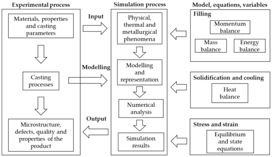
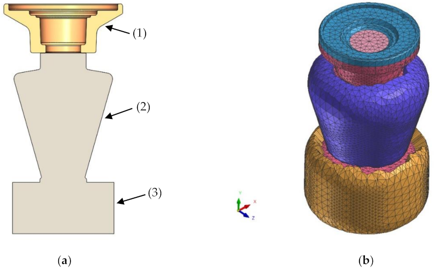
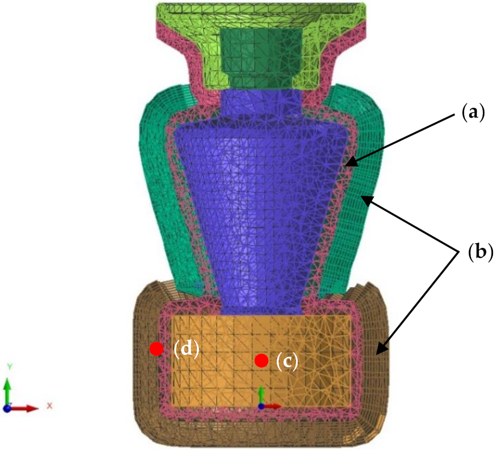
2.1. Numerical Simulation

Numerical simulations (flow and solidification analysis) and experimental trials were performed to compare shrinkage porosity results and temperature evolution during cooling, enabling the improvement of the model input parameters, such as thermal properties and casting parameters. Shrinkage porosity prediction was compared with the trial results to understand how the simulation model represented them. ProCAST^® 16.0.1, (ESI Group, Madrid, Spain) was the selected software to perform finite element analysis due to its great potential regarding the recreation of the real process and the good correlations confirmed by the foundry industry. A cylinder with a 93 mm diameter and 47 mm tall was selected for casting. Figure 2a shows the assembly in SolidWorks^® 2021 SP05.1 (Dassault Systèmes, Vélizy, France) of a part, including a conic gating system and pouring cup.

In the ProCAST^® software, the assembly follows the mesh size distribution specified in

Table 1. Element size distribution.

Tetrahedral Elements Size (mm)
Cast	10
Ceramic shell	6.5
Wool blanket	6.5

.

This element size distribution generated a model composed of 25,042 2D elements, 135,792 3D elements, and 48,054 nodes, as shown in Figure 2b. The chosen mesh density allowed for accurate results while optimising the processing time as far as possible.

In this study, ASTM F75 Co-Cr alloy (Zollern & Comandita, Maia, Portugal) was used.

Table 2. Chemical composition of ASTM F75 Co-Cr alloy.

Element	Content
Cr	27–30%
Mo	5–7%
Ni	<0.5%
Fe	<0.75%
C	<0.35%
Si	<1.0%
Mn	<1.0%
W	<0.2%
P	<0.02%
S	<0.01%
N	<0.25%
Al	<0.1%
Ti	<0.1%
B	<0.01%
Co	Bal.

presents chemical composition, where the highest concentrations are chromium and molybdenum in a cobalt base alloy.

Thermophysical parameters, such as density, thermal conductivity, enthalpy, viscosity, and solidus and liquidus temperatures used in the first iteration of the numerical simulation were based on the ProCAST^® software database. However, to better understand the influence of the heat transfer coefficient (HTC) between ceramic shells and alloy, thermal conductivity, and enthalpy of ASTM F75 alloy on the results, other values were investigated, as shown in Figures 4, 5, and 7. Further analysis will be presented in Section 3.1.

The variation of density, thermal conductivity, and enthalpy as a function of temperature in the range of 30 °C to 1700 °C is shown in Figure 3, Figure 4 and Figure 5. It is seen that as temperature rises, density decreases. This effect is quite noticeable between solidus and liquidus temperature. Thermal conductivity linearly increases from room temperature up to the solidus point. During the transition phase solidus-liquidus, the thermal conductivity decreases quickly and after the liquidus point, it increases once more. On the other hand, enthalpy increases from room temperature up to 1700 °C. Slope enthalpy increases significantly between the phase transition.

The thermal conductivity 1 (Figure 4) is the recommended curve for investment casting simulations by ProCAST^® software. The other two curves were created to evaluate the influence of this parameter on the simulation results. The thermal conductivity of curve 2 is half of curve 1, and the thermal conductivity of curve 3 is double of curve 1.

In ProCAST^® software, it is possible to generate the thermal properties of the alloy based on its chemical composition and cooling rate. The enthalpy curves 1, 2, and 3 were generated with three different cooling rates, Figure 5.

Figure 6 shows the variation of viscosity as a function of temperature, where it can be concluded that viscosity decreases with temperature rise.

The ASTM F75 alloy solidus temperature considered in this work was 1275 °C and the liquidus temperature was 1382 °C. These values, as well as density and viscosity curves were unchanged during those several iterations. The initial temperatures defined for the beginning of the simulation (at t = 0 s) were: 1000 °C for the ceramic shell, pouring cup, and wool blanket, and 1550 °C for the alloy.

The chosen values (based on ProCAST^® software for this type of simulations) for heat transfer coefficient/interface condition between:

• Ceramic shell and pouring cup were 50 W/m²K
• Ceramic shell and wool blanket were 20 W/m²K

The interface between the alloy and ceramic shell is represented by a variable that is temperature dependent, as shown in Figure 7. The heat transfer coefficient 1 is the recommended curve for investment casting simulations by ProCAST^® software. The other two curves were created to evaluate the influence of this parameter on the simulation results. The heat transfer coefficient of curve 2 is half of curve 1, and the HTC of curve 3 is double curve 1.

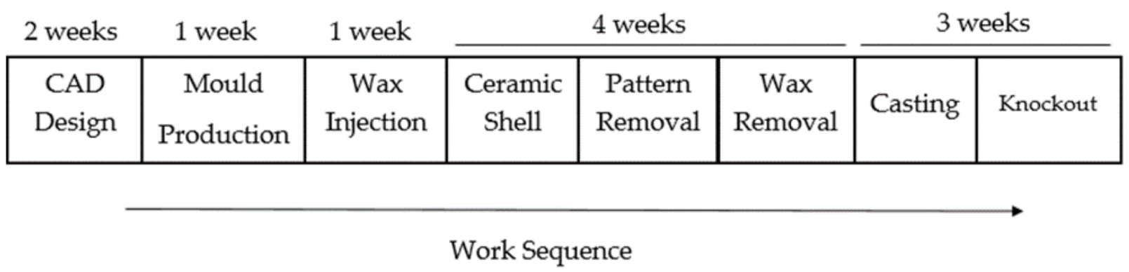
2.2. Investment Casting

2.2.1. Ceramic Shell Production

To compare numerical models and experimental results, several specimens were prepared. This preparation involves several steps, as described in Figure 8.

First, it was necessary to have a 3D-printed, accurate stereolithography (SL) pattern that would recreate the metal part, considering double shrinkage for wax and metal. With this pattern, it was then possible to obtain the mould where the wax pattern was injected. This mould produced several wax patterns, which were used for creating the ceramic shell moulds, a process that includes several steps. It was necessary to dip the wax pattern in a ceramic slurry and then a thin stucco (which thickness increases with the subsequent number of layers) was sprinkled over it to form the ceramic shell. The first layer was in contact with the metal surface part, containing materials with slightly different properties (includes grain refiner) and higher viscosity when compared with the following layers. The main reason for this is that the first layer plays a key role in grain size and roughness control. It is necessary to dry the model for a few hours before applying slurry for a new layer. After 7/8 layers, when the desired thickness is obtained, the shell mould was sent to flash fire dewaxing and sintering. Afterward, a fibrous ceramic wool blanket was applied around the shell mould (Figure 9). This blanket retains the heat in the shell mould and part, increasing the solidification time inside the chamber. Before pouring the metal, the ceramic shell (with the wool blanket surrounding it) was pre-heated at approximately 1000 °C.

After these complex procedures, the ceramic shell was ready for casting. The materials used to prepare the set of wax model, shell mould, and blanket are listed in

Table 3. Materials used to prepare the set of wax model, shell mould, and thermal blanket.

Material Information
Wax	PARACAST FW 13.070
Ceramic slurry	Levasil colloidal silica + ZrSiO4 (first layers) and levasil colloidal silica + SiO2 (following layers)
Stuccos	Zircon (first layer) and AlSi (in the following layers)
Wool blanket	Super wool plus density: 96 kg/m3 and 13 mm of thickness

.

A vacuum furnace (INEGI, Porto, Portugal) equipped with high frequency (50 kHz) induction heating in the melting chamber and electromagnetic stirring in the pouring chamber setup was used for metal gravity pouring. Casting equipment encompasses a vacuum chamber, a magnetic field inductor, an induction coil, cooling channels, and a pneumatic cylinder that provides position control of the cast during several points of the process.

To validate the model under development, the same parameters were applied to a complex geometry, more specifically, hip prostheses (Figure 10). Medical parts have high-quality standards, requiring a low defect content. To verify the defect prediction capacity of the numerical model, several hip samples were manufactured and a macro-analysis was performed.

2.2.2. Thermocouple Positioning

To obtain cooling behaviour information, thermocouples were placed in specific positions. The first one, at the casting centre, allows the retrieval of alloy thermal information. The second provides thermal information on the frontier between the shell mould and wool blanket. Two high-temperature thermocouples (S type) were used in this experience, as seen in Figure 11. One was positioned in the cylinder centre so that the alloy temperature could be registered. This specific thermocouple was inserted inside a quartz tube to reduce reading interferences and protect it from the poured metal. The second thermocouple was positioned inside the wool blanket. The data were then acquired using the LabVIEW 2012 SP1 software (NI, Austin, TX, USA).

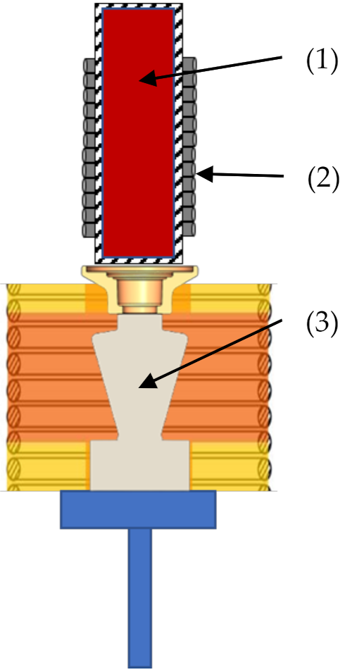
2.2.3. Metal Pouring

The alloy charge for casting and shell mould were preheated for 4 h at 250 °C and 1000 °C, respectively. Then, these materials were transferred rapidly and manually to the casting furnace, Figure 12. The ASTM F75 Co-Cr ingot (Zollern & Comandita, Maia, Portugal) with 73 mm of diameter and 160 mm of height was melted by induction and the temperature was raised up to 1500–1600 °C. The pouring of the Co-Cr alloy occurred at t = 373 s. This time was also considered in the simulation in order to reproduce the case study in a more realistic way. During the pouring and cooling steps, the alloy was subjected to a vacuum environment (0.1 mbar). With this process, there is a lower chance of atmospheric reaction (oxides formation or hydrogen absorption). Twenty min after pouring, the casting and ceramic shell were removed from the vacuum furnace and cooled at room temperature. After that, the ceramic shell was cracked by a knockout process and the cast was cleaned.

3. Results and Discussion

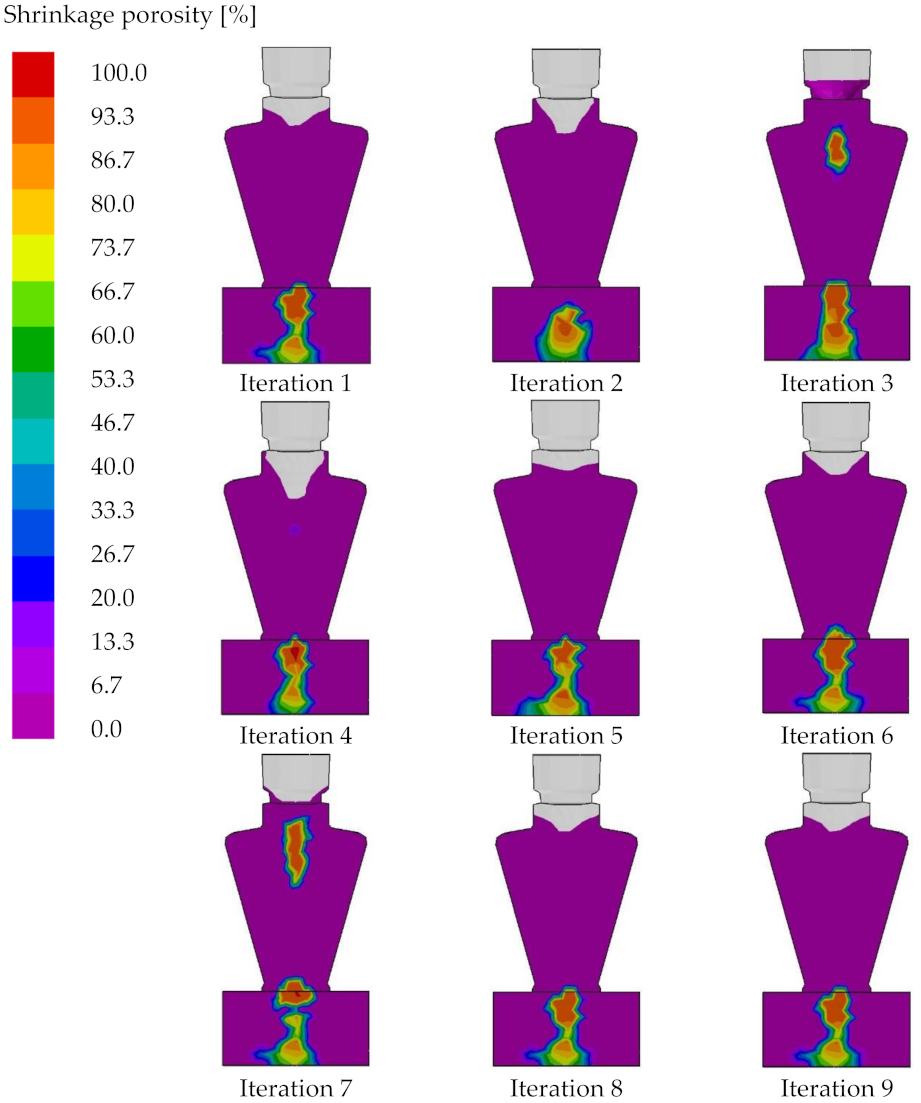
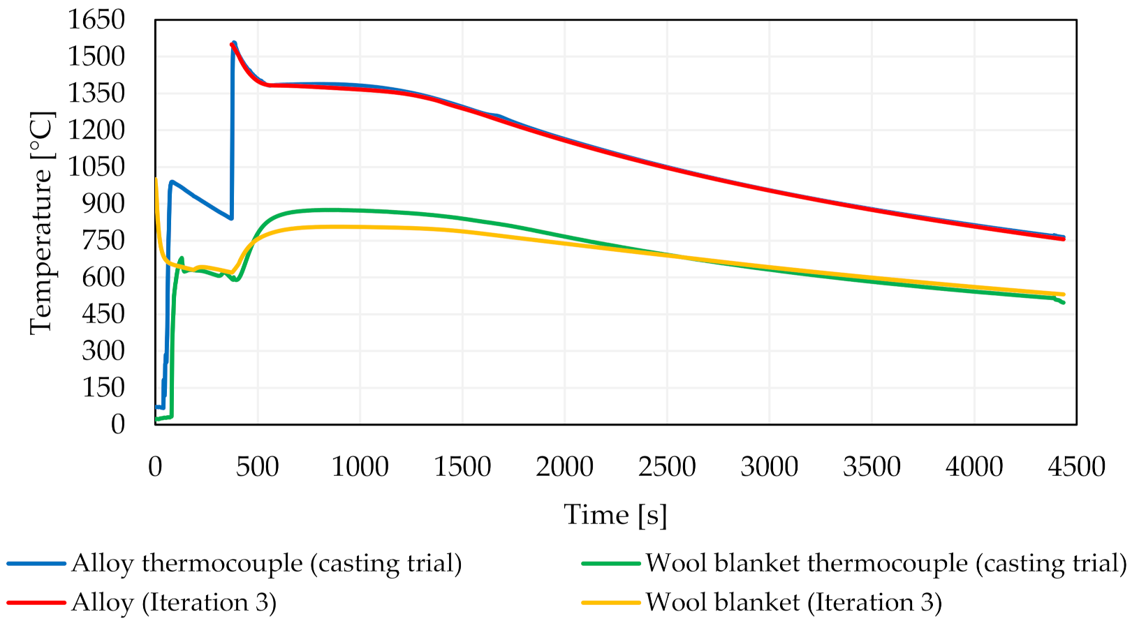
3.1. Numerical Simulation Results

In the course of this work, some initial assumptions were made according to the ProCAST^® software recommended values. However, a set of iterations (

Table 4. Set of iterations to evaluate the influence of enthalpy, thermal conductivity, heat transfer coefficient, and emissivity parameters.

Iteration Number	Enthalpy Curve	Thermal Conductivity Curve	Heat Transfer Coefficient Curve	Emissivity
IT1	curve 1 (Figure 5)	curve 1 (Figure 4)	curve 1 (Figure 7)	0.9
IT2	curve 2 (Figure 5)	curve 1 (Figure 4)	curve 1 (Figure 7)	0.9
IT3	curve 3 (Figure 5)	curve 1 (Figure 4)	curve 1 (Figure 7)	0.9
IT4	curve 1 (Figure 5)	curve 2 (Figure 4)	curve 1 (Figure 7)	0.9
IT5	curve 1 (Figure 5)	curve 3 (Figure 4)	curve 1 (Figure 7)	0.9
IT6	curve 1 (Figure 5)	curve 1 (Figure 4)	curve 2 (Figure 7)	0.9
IT7	curve 1 (Figure 5)	curve 1 (Figure 4)	curve 3 (Figure 7)	0.9
IT8	curve 1 (Figure 5)	curve 1 (Figure 4)	curve 1 (Figure 7)	0.7
IT9	curve 1 (Figure 5)	curve 1 (Figure 4)	curve 1 (Figure 7)	0.5

) was established in order to evaluate the influence of some parameters. The choice of these parameters (enthalpy, thermal conductivity, heat transfer coefficient and emissivity) was based on past experiences of the team with similar simulation studies. The starting point (iteration 1) was based on ProCAST^® software recommendations for this type of simulation and the following iterations were performed in order to evaluate the influence of each parameter. As shown in Section 2.1, three curves/values were studied for each parameter.

Figure 13 shows the influence of the enthalpy curve on the cooling behaviour of the alloy and wool blanket. It can be seen that in iteration 3, the solidus-liquidus transition is shorter (approximately 700 s) when compared with iterations 1 and 2, once the energy to transit from liquidus to solidus temperatures is lower. It can also be concluded that with a lower enthalpy value (e.g., enthalpy curve 1 vs. enthalpy curve 2), for the same amount of mass and energy lost, the decay of temperature is greater with a lower enthalpy value, which is the case of iteration 2. It is also possible to notice that, with a higher alloy temperature, a higher wool blanket temperature is observed.

Figure 14 shows the effect of the thermal conductivity curve on the alloy and wool blanket cooling behaviour. It is possible to infer that with the increase of conductivity (iteration 5), the cooling of the alloy and the wool blanket is higher.

Figure 15 depicts the effect of the HTC curve on the alloy and wool blanket cooling behaviour. It is clear that with the increase of the heat transfer coefficient, the cooling in both alloy and wool blanket is higher, as expected. However, this behaviour is only observed for temperatures below the solidification temperature.

On the other hand, as shown in Figure 16, the emissivity value does not have influence on cooling behaviour of the alloy and wool blanket.

It is possible to observe, in Figure 17, a pattern of shrinkage porosity in the centre of the part in all iterations. In contrast, iterations 3 and 7 predict that there is a higher probability of shrinkage porosity at the top of the gating system and in iteration 4 there is a small probability of shrinkage porosity at the top of gating system. It is also important to mention that iteration 2 is the only one that does not predict shrinkage porosity in the transition zone between the gating system and part. These results are consequence of thermal properties of the ASTM F75 alloy and heat transfer coefficient between alloy and ceramic shell.

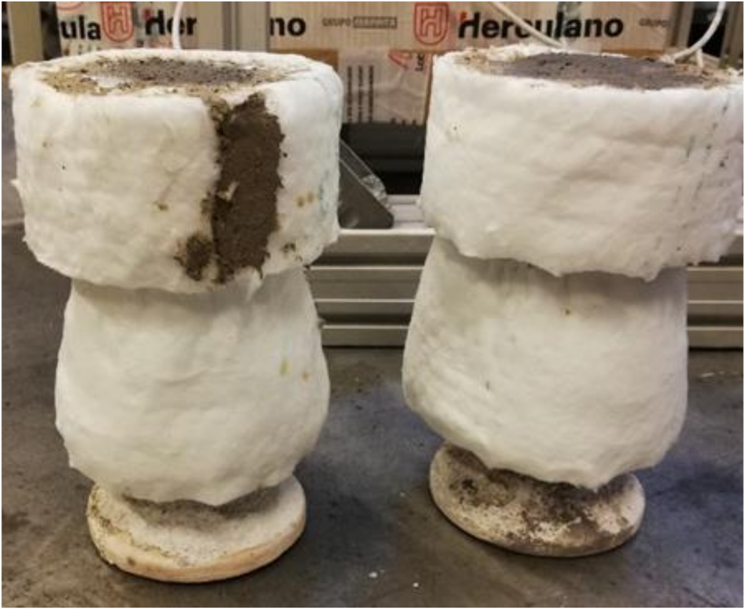
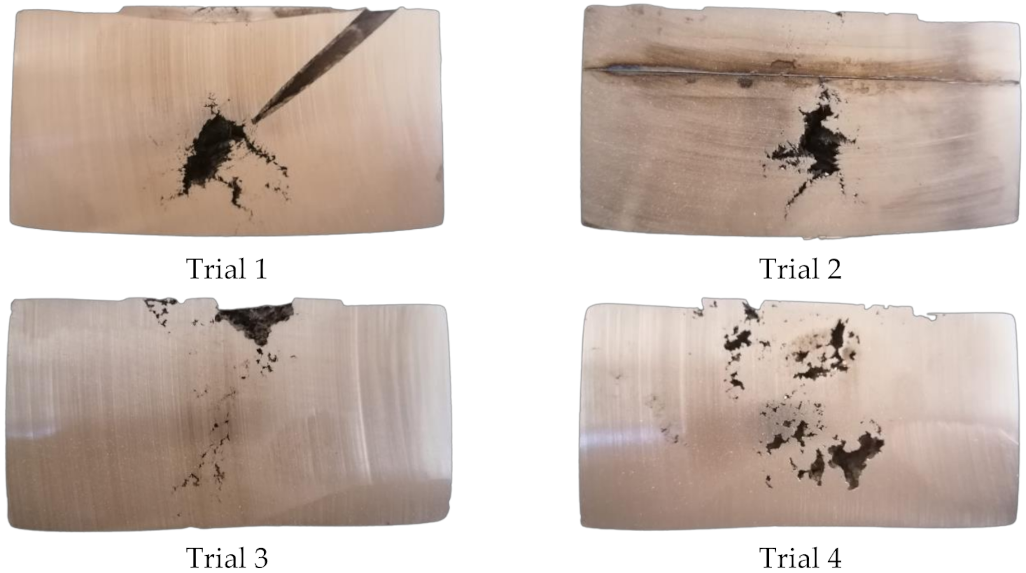
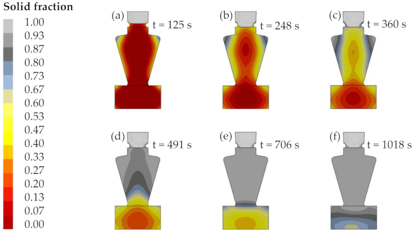
3.2. Cylinder with a Conic Gating System

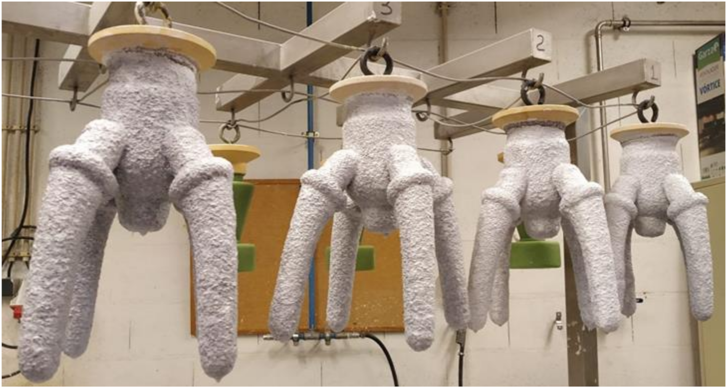
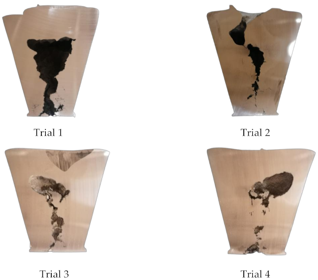
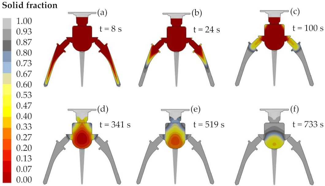
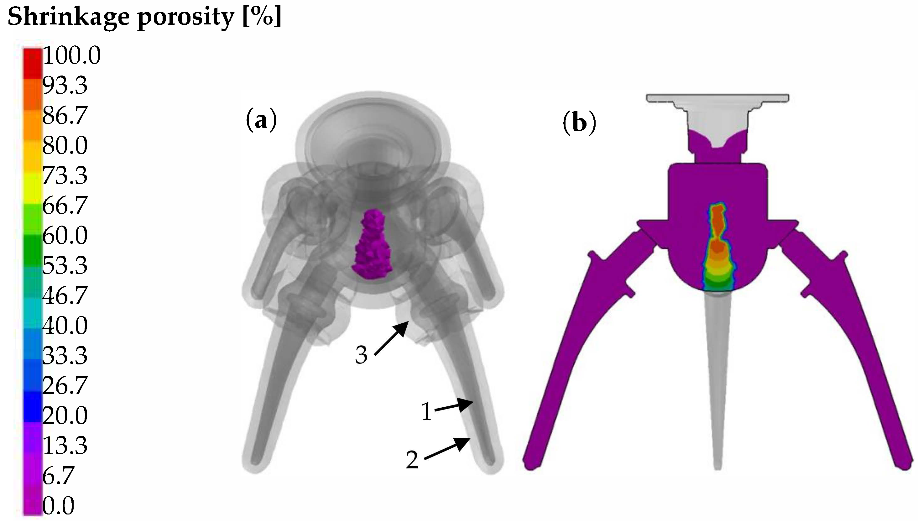
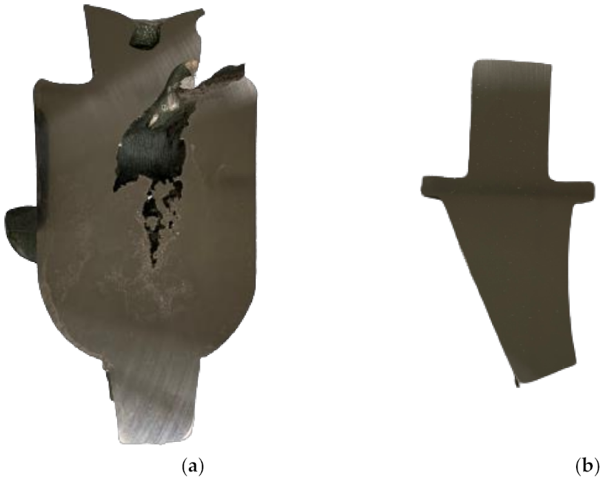
Based on results of Section 3.1, all the curves were compared with the experimental one in order to evaluate if any of them represented the experimental trial curve. As it is shown in Figure 18, the temperature evolution in the numerical simulation (iteration 3) and experimental trial demonstrates that temperature trends are similar, revealing a good correlation between the numerical model and the experimental trial.

Firstly, the temperature read on the thermocouples increases, as this corresponds to the moment when they are applied in the positions previously specified, being in contact with hot surfaces. The temperature decrease between 75 and 370 s corresponds to the time needed to vacuum in the induction furnace and fusion. It is important to mention that the inductive heat only affects the alloy charge. After the fusion, the metal pours over the shell mould due to the gravity effect, increasing the thermocouples reading temperature. Lastly, the temperature readings decrease, which correspond to the alloy and shell mould cooling.

To validate this numerical model, it was necessary to analyse and compare shrinkage porosity results from iteration 3 (Figure 17) with the results retrieved from the real casts. The cross-section of the gating system and cast part for the four experimental trials performed, Figure 19 and Figure 20, confirm the simulation results. It is important to refer that numerical simulation predicts where shrinkage porosity might occur in terms of probability (%), which means that is possible to obtain slightly different results regarding the location and size of those defects.

To explain why shrinkage porosity is observed in the centre of the gating system and part, the solidification process of the casting was analysed. It is seen in Figure 21a that after 125 s (about 2 min) of the pouring process, both the part and gating system are still liquid. Figure 21b,c illustrate that the solidification process starts from the external surfaces to the centre and after 360 s (6 min); in Figure 21c, the centre of the part is still liquid, whereby the gating system is already solid in Figure 21d. Figure 21e,f confirm that the gating system solidifies later.

This path of solidification shows that the possibility of shrinkage porosity formation at the centre of the gating system and part is highly possible, as seen in iteration 3 of Figure 17.

3.3. Hip Prostheses

Applying the optimised conditions (iteration 3 from Section 3.1) to the numerical model of the hip prostheses, it was possible to obtain the results in Figure 22, which show the solidification process of the hip prostheses cast. It is seen in Figure 22a that after 8 s of the pouring process, both parts and the gating system are still liquid. Figure 22b,c illustrate that the solidification path starts from the bottom to the top of the prosthesis part, towards the gating system and after 341 s (Figure 22d) the centre of the gating system is still liquid, whereby hip prostheses are already solid. Figure 22e,f show that the bottom part of the gating system is the last zone to solidify. Figure 23 expects shrinkage porosity at the centre of the gating system, as predicted by the solidification path in Figure 22.

To compare the experimental results with numerical ones, two pouring trials were performed, and similar results were achieved on both. Then, hip prostheses were separated from the gating system, and both were sectioned and polished as shown in Figure 24. It was not possible to analyse an entire hip prosthesis section due to high toughness and cutting equipment limitations (small size of the sample), which makes precision cutting a difficult task. However, the critical zone (last zone to solidify) was analysed as observed in Figure 24b. As it can be noticed, there is no shrinkage porosity in the hip prostheses; however, there is a significant hole in the gating system centre, as predicted by the ProCAST^® numerical model.

4. Conclusions

In the course of this study, mould filling and solidification analysis were performed for the CoCr alloy using ProCAST^® simulation software. Adopting the same geometry, experimental trials were performed to compare numerical and experimental results. The following conclusions were drawn:

• It is possible to match numerical information with experimental results by controlling the thermal properties of the CoCr alloy, the interface between volumes, as well as heat conditions of the numerical model.
• Thermal properties are essential and can significantly influence numerical results. For any numerical simulation, there is a great need to study the alloy properties to achieve reliable results.
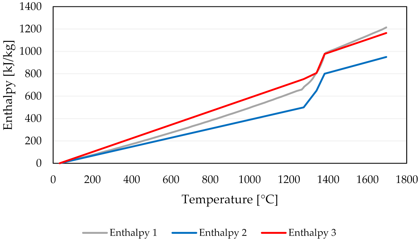
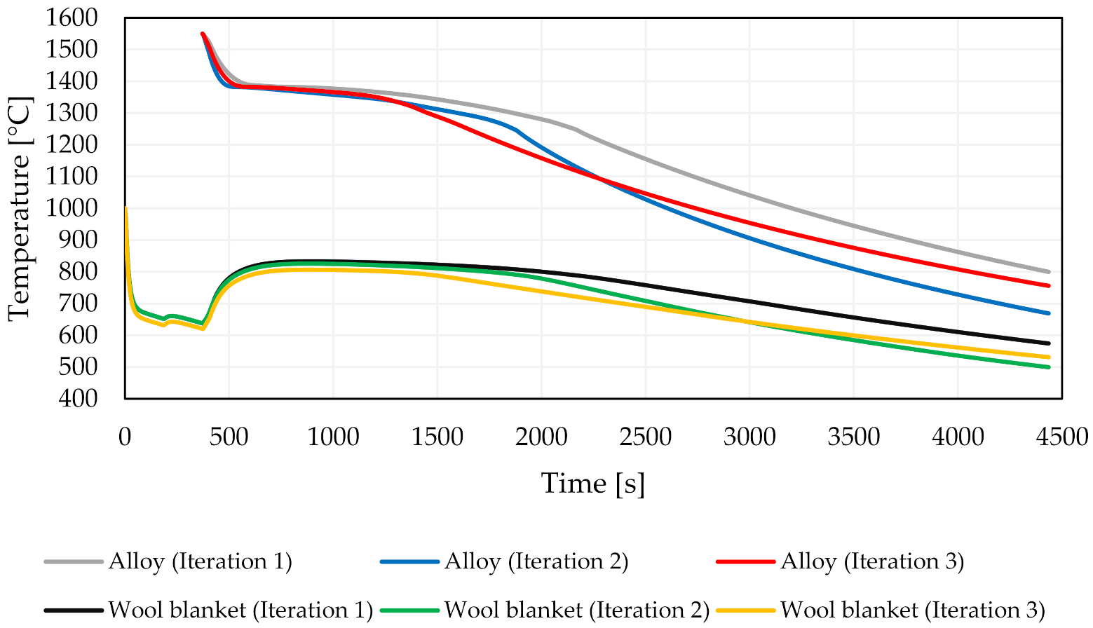
• The enthalpy curve plays a very important role in predicting shrinkage porosity and temperature behaviour. With a lower enthalpy value, for the same amount of mass and energy lost, and the decay of temperature is higher.
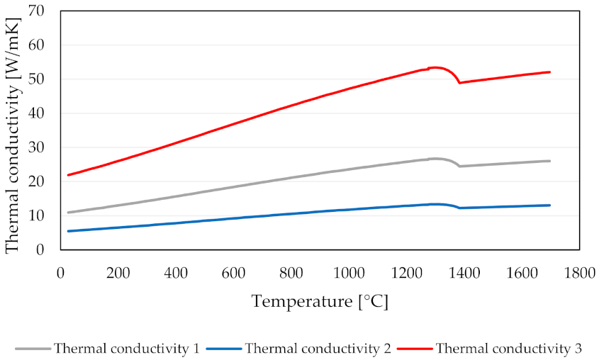
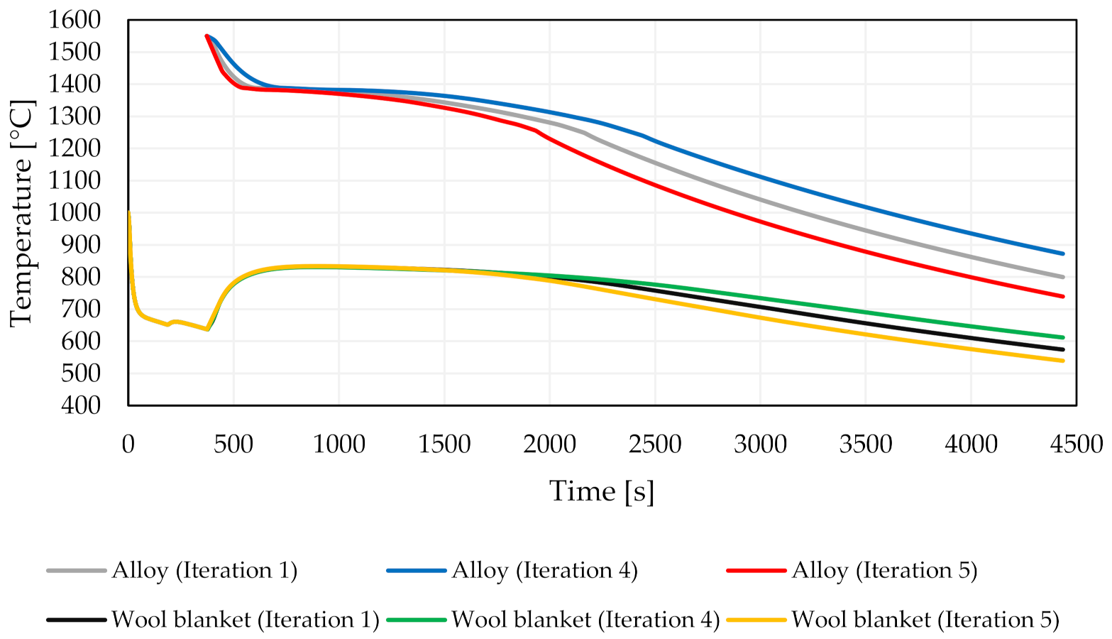
• With an increase in conductivity, the alloy and wool blanket cooling level is higher, proving that thermal conductivity influences numerical simulation results.
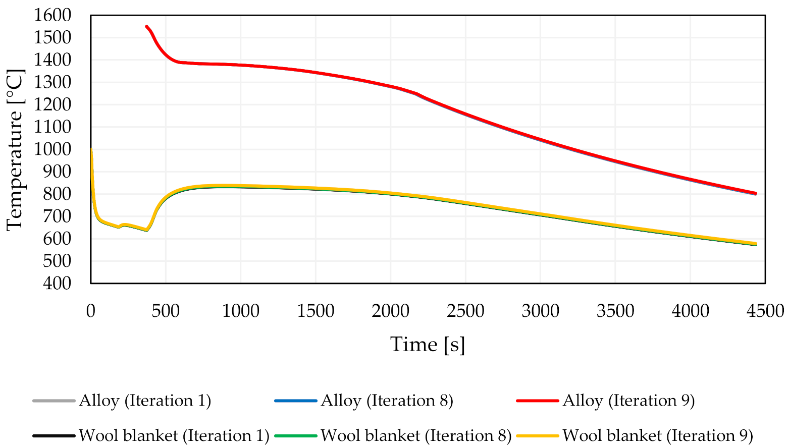
• Emissivity has virtually no influence on metal cooling behaviour.
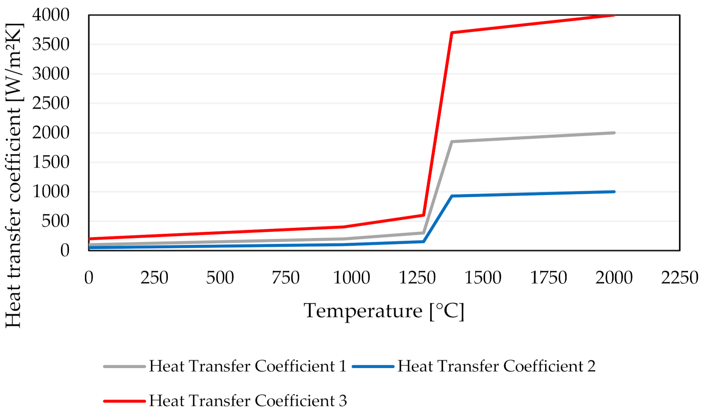
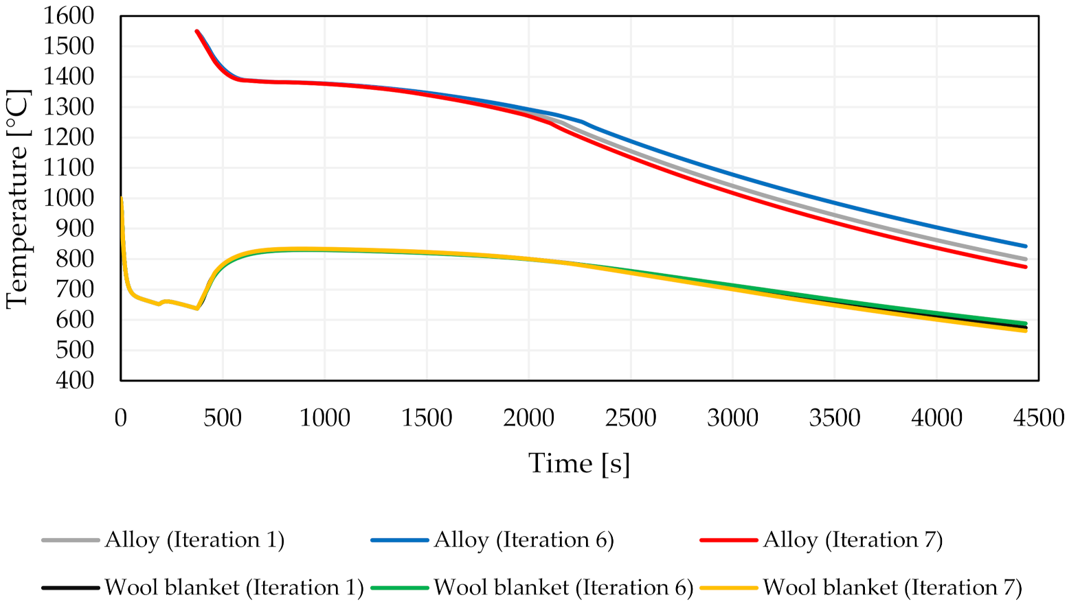
• Heat transfer coefficients between the alloy and the ceramic shell only affect metal cooling behaviour below the solidus temperature.
• It is possible to develop a model that can predict shrinkage porosity defects in casts with different geometries, if the same alloy thermal properties and same thermal conditions are applied.

References

1. Milošev, I. CoCrMo Alloy for biomedical applications. In Biomedical Applications; Djokić, S.S., Ed.; Springer: Boston, MA, USA, 2012; pp. 1–72. [Google Scholar]
2. Giacchi, J.V.; Morando, C.N.; Fornaro, O.; Palacio, H.A. Microstructural characterization of as-cast biocompatible Co-Cr-Mo alloys. Mater. Charact. 2011, 62, 53–61. [Google Scholar] [CrossRef]
3. Escobedo, J.; Méndez, J.; Cortés, D.; Gómez, J.; Méndez, M.; Mancha, H. Effect of nitrogen on the microstructure and mechanical properties of a Co–Cr–Mo alloy. Mater. Des. 1996, 17, 79–83. [Google Scholar] [CrossRef]
4. Fleming, T.J.; Kavanagh, A.; Duggan, G.; O’Mahony, B.; Higgens, M. The effect of induction heating power on the microstructural and physical properties of investment cast ASTM-F75 CoCrMo alloy. J. Mater. Res. Technol. 2019, 8, 4417–4424. [Google Scholar] [CrossRef]
5. Park, J.B.; Jung, K.H.; Kim, K.M.; Son, Y.; Lee, J.I.; Ryu, J.H. Microstructure of as-cast Co-Cr-Mo alloy prepared by investment casting. J. Korean Phys. Soc. 2018, 72, 947–951. [Google Scholar] [CrossRef]
6. Lewis, R.W.; Ravindran, K. Finite element simulation of metal casting. Int. J. Numer. Methods Eng. 2000, 47, 29–59. [Google Scholar] [CrossRef]
7. Sutiyoko, S.; Suyitno, D.; Mahardika, M.; Syamsudin, A. Prediction of shrinkage porosity in femoral stem of titanium investment casting. Arch. Foundry Eng. 2016, 16, 157–162. [Google Scholar] [CrossRef] [Green Version]
8. Khan, M.A.A.; Sheikh, A.K. Simulation tools in enhancing metal casting productivity and quality: A review. Proc. Inst. Mech. Eng. Part B J. Eng. Manuf. 2016, 230, 1799–1817. [Google Scholar] [CrossRef]
9. Zhu, J.Z.; Guo, J.; Samonds, M.T. Numerical modeling of hot tearing formation in metal casting and its validations. Int. J. Numer. Methods Eng. 2011, 87, 289–308. [Google Scholar] [CrossRef]
10. Pattnaik, S.; Karunakar, D.B.; Jha, P.K. Developments in investment casting process—A review. J. Mater. Processing Technol. 2012, 212, 2332–2348. [Google Scholar] [CrossRef]
11. Menne, R.; Weiss, U.; Brohmer, A.; Walter, A.; Weber, M.; Oelling, P. Implementation of casting process simulation for increased engine performance and reduced development time and costs—Selected examples from FORD R and D engine projects. In Proceedings of the 28th International Vienna Motor Symposium, Vienna, Austria, 26–27 April 2007. [Google Scholar]
12. Fu, M.W.; Yong, M.S. Simulation-enabled casting product defect prediction in die casting process. Int. J. Prod. Res. 2009, 47, 5203–5216. [Google Scholar] [CrossRef]
13. Huang, P.-H.; Lin, C.-J. Computer-aided modeling and experimental verification of optimal gating system design for investment casting of precision rotor. Int. J. Adv. Manuf. Technol. 2015, 79, 997–1006. [Google Scholar] [CrossRef]
14. Im, D.J.; Hong, J.S.; Kang, I.S. Numerical analysis on the enhancement of molten steel stirring by magnetic field strength control. Comput. Fluids 2012, 70, 13–20. [Google Scholar] [CrossRef]
15. Wang, Y.-C.; Li, D.; Peng, Y.-H.; Zeng, X.-Q. Numerical simulation of low pressure die casting of magnesium wheel. Int. J. Adv. Manuf. Technol. 2007, 32, 257–264. [Google Scholar] [CrossRef]
16. Shepel, S.V.; Paolucci, S. Numerical simulation of filling and solidification of permanent mold castings. Appl. Therm. Eng. 2002, 22, 229–248. [Google Scholar] [CrossRef]
17. ProCAST®; Version 16.0.1. Information Extracted from ProCAST® Database; ESI Group: Rungis, France, 2020.
Figure 1. Flowchart for the process, modelling, simulation, and output variables (adapted from [12]).
Metals 12 00351 g001
Figure 2. Design of the casting assembly. (a) Cross section view in SolidWorks® and (b) model mesh distribution in ProCAST® software. (1) Pouring cup, (2) gating system, and (3) part.
Metals 12 00351 g002
Figure 3. Density as a function of temperature [17].
Metals 12 00351 g003
Figure 4. Thermal conductivity as a function of temperature [17].
Metals 12 00351 g004
Figure 5. Enthalpy as a function of temperature in the first and last iterations [17].
Metals 12 00351 g005
Figure 6. Viscosity as a function of temperature [17].
Metals 12 00351 g006
Figure 7. ASTM F75—Ceramic Shell interface condition. Heat transfer coefficient as function of temperature.
Metals 12 00351 g007
Figure 8. Timeline of the key steps of this work.
Metals 12 00351 g008
Figure 9. Thermal blanket applied around ceramic shell.
Metals 12 00351 g009
Figure 10. Hip prostheses shell mould.
Metals 12 00351 g010
Figure 11. Positioning thermocouples in the current study (cross section view). (a) Ceramic shell, (b) wool blanket, (c) positioning the thermocouple on the alloy (centre part), and (d) positioning the thermocouple on the wool blanket.
Metals 12 00351 g011
Figure 12. Vacuum furnace sketch. (1) Metal ingot, (2) induction coil, and (3) ceramic shell mould.
Metals 12 00351 g012
Figure 13. Evaluation of the influence of enthalpy on the alloy and wool blanket temperature results.
Metals 12 00351 g013
Figure 14. Evaluation of the influence of thermal conductivity on the alloy and wool blanket temperature results.
Metals 12 00351 g014
Figure 15. Evaluation of the influence of heat transfer coefficient on the alloy and wool blanket temperature results.
Metals 12 00351 g015
Figure 16. Evaluation of the influence of emissivity on the alloy and wool blanket temperature results.
Metals 12 00351 g016
Figure 17. Shrinkage porosity prediction for both gating system and part for iteration 1 to 9.
Metals 12 00351 g017
Figure 18. Temperature evolution in the casted part and in the insulation wrap, obtained from experimental trial and simulation.
Metals 12 00351 g018
Figure 19. Visual inspection of the gating system, trial 1 to 4 (cross-section cut).
Metals 12 00351 g019
Figure 20. Visual inspection of the part, trial 1 to 4 (cross-section cut).
Metals 12 00351 g020
Figure 21. Solidification process of the casted part (cross section view). (a) 125 s; (b) 248 s; (c) 360 s; (d) 491 s; (e) 706 s; (f) 1018 s.
Metals 12 00351 g021
Figure 22. Solidification process of the hip prostheses model (cross section view). (a) 8 s; (b) 24 s; (c) 100 s; (d) 341 s; (e) 519 s; (f) 733 s.
Metals 12 00351 g022
Figure 23. Hip prostheses shrinkage porosity prediction with PROCAST® software. (a) Isometric view and (b) cross section view in plane XY. (1) Hip prosthesis, (2) ceramic shell, and (3) wool blanket.
Metals 12 00351 g023
Figure 24. Shrinkage porosity of hip prostheses model. (a) Gating system and (b) hip prosthesis cross section view.
Metals 12 00351 g024