Article

Design Optimization of a Single-Strand Tundish Based on CFD-Taguchi-Grey Relational Analysis Combined Method

by
Dong-Yuan Sheng
1,2
1
Department of Materials Science and Engineering, Royal Institute of Technology, 10044 Stockholm, Sweden
2
Westinghouse Electric Sweden AB, 72163 Västerås, Sweden
Metals 2020, 10(11), 1539; https://doi.org/10.3390/met10111539
Submission received: 18 October 2020 / Revised: 13 November 2020 / Accepted: 16 November 2020 / Published: 19 November 2020
(This article belongs to the Special Issue Numerical Modelling in Steel Metallurgy)

Abstract

:
A novel digital design methodology that combines computational fluid dynamics (CFD) modelling and Taguchi-Grey relational analysis method was presented for a single-strand tundish. The present study aimed at optimizing the flow control device in the tundish with an emphasis on maximizing the inclusion removal rate and minimizing the dead volume fraction. A CFD model was employed to calculate the fluid flow and the residence-time distribution of liquid steel in the tundish. The Lagrangian approach was applied to investigate the behavior of non-metallic inclusions in the system. The calculated residence-time distribution curves were used to analyze the dead volume fraction in the tundish. A Taguchi orthogonal array L9(3^4) was used to analyze the effects of design factors on both single and multiple responses. Moreover, for the purpose of meeting the multi-objective target functions, grey relational analysis and analysis of variance were used. The optimum positions of the weir and the dam were obtained based on the design targets. A special focus of this study was to demonstrate the capabilities of the Taguchi-Grey relational analysis method as a powerful means of increasing the effectiveness of CFD simulation.

1. Introduction

The tundish, working as a buffer and distributor of liquid steel between ladle and continuous casting (CC) molds, plays a key role in affecting the performance of the CC machine, solidification of liquid steel, quality, and productivity [1,2]. Tundish design varies widely from plant to plant, owing to the differences in the end products, number of strands, and operating parameters. An optimum tundish design aims at providing maximum opportunity for the control of liquid steel flow, heat transfer, mixing, and inclusion removal. Considerable efforts have been made in both academia and industry over many decades to fully exploit and enhance the metallurgical performance of the tundish [3,4]. Among this, computational fluid dynamics (CFD) and water model experiments have been considered as useful and promising tools that can accurately predict many phenomena of practical interest in tundish. A summary of the previous published modelling works can be found in the references [5,6].
The Taguchi method is a broadly accepted method of design of experiments (DOE), which has been proven in producing high-quality products at subsequently low cost. It is considered to be highly effective through following two aspects: (i) robust design—the approach of finding optimum design factors that lead to economic designs with low variability; (ii) parameter design—the process of identifying the settings of the design factors that reduce the design sensitivity due to the source variation. Taguchi designs use orthogonal arrays to estimate the factors’ effect on the response mean and variation. An orthogonal array means the design is balanced so that factor levels are equally weighted. Thus, each factor can be assessed independent from the other factors. It reduces both time and cost associated with the design trials when fractional factorial designs are used [7,8].
With the emphasis on superior steel quality, two indexes can be applied to evaluate the tundish design: (i) inclusion remove rate (IRR); (ii) dead volume fraction (DVF). Dead zones can slowly mix and contaminate the newly incoming steel. The inclusion removal rate is an index related to the steel quality. The proper implementation of flow control devices (FCD) ensures the homogeneity of liquid steel and enhances the inclusion removal. More specifically, it is necessary to obtain the optimum FCD designs in tundish with high IRR and low DVF.
With focus on optimization of FCD design within the tundish, engineers have carried out a large number of investigations using experimental and numeric approaches in order to address the relevant design parameters that govern the desirable performance features. The literature on tundish design is summarized in Table 1 [9,10,11,12,13,14,15,16,17,18,19,20,21,22,23,24]. The aforementioned studies have led to considerable improvements in understanding various transport processes associated with tundish operations, aiming for the optimal tundish design. However, few studies have employed a systematic approach to analyze how the multiple design targets can be assessed simultaneously.
Normally, engineers can only simulate the process response through a one design factor at a time strategy, while holding other parameters at a constant level. Thus, interaction effects between dependent design factors are disregarded. Recently, attention has been drawn to systematic design optimization with multiple design factors. This systematic approach is called design of experiments. It allows explaining the interaction of design factors and the way the total system works by using statistical analyses [25].
The objective of this study was to develop a digital design methodology that combined CFD modelling and the Taguchi method for a single-strand tundish. A Taguchi orthogonal array L9(3^4) was used to analyze the effects of design parameters on both single (IRR, DVF) and multiple responses (IRR + DVF). Grey relation analysis (GRA) was used for the multiple-response optimization. Analysis of variance (ANOVA) was also carried out for finding out the contribution and impact of each design factor towards the responses. The hydrodynamic modeling result allows to optimize flow control device in the tundish with the emphasis on high IRR and low DVF. The optimum positions of the weir and the dam were obtained based on the design targets. This study demonstrated that the digital design, using the advanced computational methods, can be a significant technology for particles of industrial design. Moreover, the digital design will become an important part for the digitalization process in the steel industry.

2. Methodology

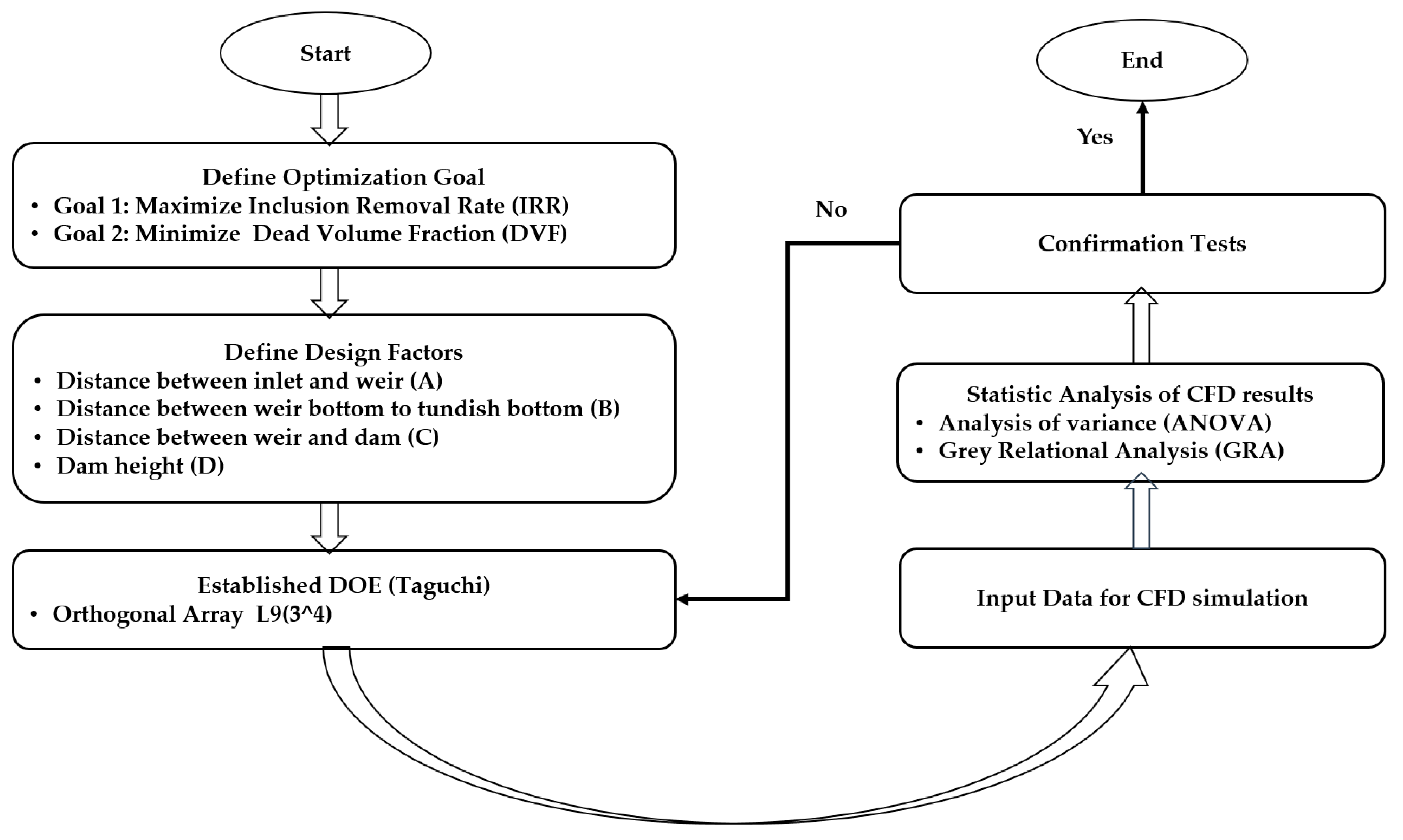
2.1. Design Objectives and Solution Strategy

A single-strand tundish (14 tons) with a submerged inlet, an outlet, a weir, and a dam was under investigation in the current work. The geometric dimensions of the tundish are illustrated in Figure 1. The liquid steel flow rate remained unchanged to keep a constant steel bath level in the tundish. To maintain chemical and thermal homogeneity, as well as promote inclusion removal in the tundish, two responses were considered:
(i)
inclusion remove rate (IRR), which is defined as (1 − inclusions reaching outlet/inclusions injected at inlet);
(ii)
dead volume fraction (DVF), which is defined as (1 − calculated mean residence time/theoretical mean residence time).
(iii)
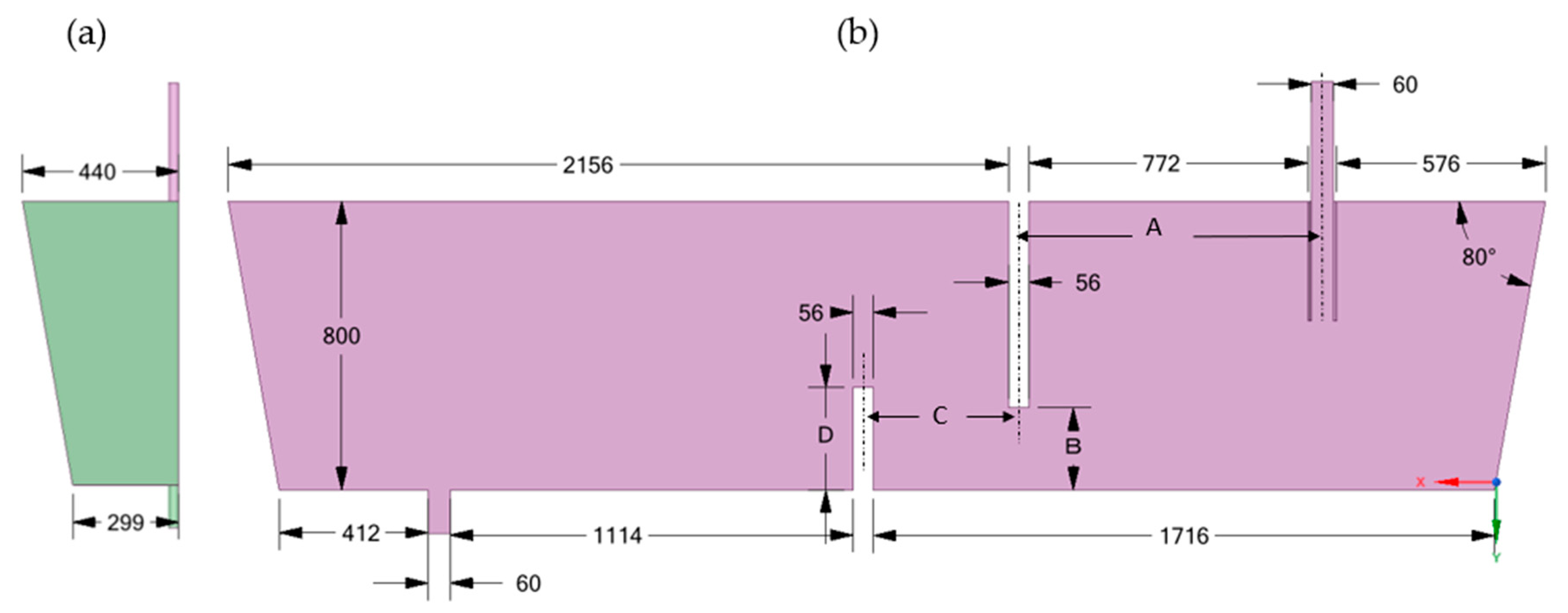
The design optimization should be able to meet the conflicting requirements, which are maximizing IRR and minimizing DVF. The design objective was to obtain the optimized values of four design factors (shown in Figure 1):
(iv)
A (distance between inlet and weir),
(v)
B (distance of tundish bottom to weir),
(vi)
C (distance between weir and dam), and
(vii)
D (dam height).
The design was optimized by combining CFD simulation and Taguchi DOE methods. The flow diagram of the design process is presented in Figure 2. Firstly, the optimization goals were set to maximize IRR and minimize DVF in the tundish. Secondly, four design factors (A, B, C, and D) were selected based on metallurgical expertise for the optimization process. Each factor was further assigned a variation domain bounded by low, medium, and high values. These variations were arranged through Taguchi orthogonal array (OA) L9(3^4) to create parametric computer-aided design (CAD) geometries, which were utilized for CFD simulations. Thirdly, CFD simulation results were post-processed through Taguchi data analysis, ANOVA, and Grey relational analysis, aiming at selecting the optimal combination of design factors. Lastly, the optimization terminated when the data-analyzed optimal design reached the design objective. Otherwise, it continued to loop with a new set of proposed design factors.

2.2. Design of Experiment

Minitab V.18 (Minitab, LLC, State College, Pennsylvania, PA, USA) software was used for DOE analysis in this study [26]. The DOE consists of four phases: planning, characterization, optimization, and verification. The multi-objective optimization was built by combining CFD simulation and design of experiment.

2.2.1. Taguchi Design

Taguchi analysis uses a classical signal-to-noise (S/N) ratio as a numerical measurement for deciding the optimal circumstances. Noise (N) is the set of uncontrolled parameters that influences the result or response. Signal (S) is the output variable or response. The S/N ratio indicates robustness of an experiment. There are three categories of S/N ratios: (i) smaller-is-better, (ii) larger-is-better, and (iii) nominal-is-best. The three S/N ratios are described in Equations (1)–(3). Depending on the application, one should firstly identify the objective function to be optimized.
smaller-is-better :   S / N = 10 log 1 n i = 1 n y i 2
larger-is-better :   S / N = 10 log 1 n i = 1 n 1 y i 2
normal-is-best :   S / N = 10 log y ¯ 2 s 2
where y is the performance characteristic value, n is the observation repeat number, and s2 is the variance.
In this work, the Taguchi orthogonal array L9(3^4) was applied to define the optimum designs regarding the selected factors. In Table 2, four factors with high, medium, and low values were considered in DOE. As suggested by the Taguchi orthogonal array, nine CFD cases (cases 1–9) were proposed with different combinations of the factor levels and displayed in Table 3. Case 0 (bare tundish) was added as a reference case.

2.2.2. Analysis of Variance

Analysis of variance (also referred to F-test) was developed by Ronald Fisher, the pioneer and innovator of the use and application of statistical methods in experimental design [27]. The criteria for determining the design factor’s effect on response function mainly rely on the magnitude of the F-value, defined in Equation (4). The design factor with the highest F-value represents the factor with the most significant effect on the response function.
F = MST/MSE
where, MST is the mean square for treatments, and MSE is the mean square for error.

2.2.3. Grey Relational Analysis

Grey relational analysis (GRA), one of the most widely used models of Grey system theory, was initially proposed by Deng [28]. GRA defines situations with no information as black and those with perfect information as white. However, neither of these idealized situations occurs in real-world problems. In fact, situations between these extremes, containing partial information, are described as being grey. A variant of the GRA model, the Taguchi-based GRA model, is nowadays very popular in engineering [29].
A multi-objective target is needed in the tundish design. To overcome the limitation of using a single response by the Taguchi method, the GRA method [30] is here employed to convert the multi-objective target into a single target optimization problem. The criteria of larger-is-better and smaller-is-better have been used to describe the inclusion removal rate and the dead volume fraction, respectively.
These factors are standard-transformed by Equations (5)–(7).
For the benefit-type factor :   x i ( k ) = x i ( k ) min x i ( k ) max x i ( k ) min x i ( k )
For the defect-type factor :   x i ( k ) = max x i ( k ) x i ( k ) max x i ( k ) min x i ( k )
For the medium-type factor :   x i ( k ) = x i ( k ) x 0 ( k ) max x i ( k ) x 0 ( k )
The grey relational grade (GRG) is calculated by the following steps:
(i)
The absolute difference of the compared series and the referential series should be obtained by Equation (8). The maximum and the minimum differences are obtained.
Δ x i ( k ) = x 0 ( k ) x i ( k )
(ii)
Calculation of the relational coefficient and relational grade by Equation (9). The distinguishing coefficient p is between 0 and 1. Typically, the distinguishing p value is set to be 0.5.
ξ i ( k ) = Δ min + p Δ max Δ x i ( k ) + p Δ max
(iii)
The grey relational grade is defined in Equation (10):
r i = w ( k ) ξ ( k )
where ξ is the Grey relational coefficient, w(k) is the weight factor; w(k) is set as 0.5 in this study.

2.3. CFD Model

2.3.1. Model Description

CFD software STAR-CCM + V.13 (Siemens PLM software, Plano, TX, USA) was used to simulate the fluid flow, the inclusion removal, and the residence-time distribution [31]. The assumptions made for the mathematical model are described below:
  • The model is based on a 3D standard set of the Navier–Stokes equations.
  • Isothermal and steady-state liquid flow is considered.
  • The motion of inclusions is simulated by solving the force balance equations.
  • The realizable k-ε model is used to describe the turbulence.
  • The free surface is flat and is kept at a fixed level. The tundish slag layer is not included.
  • The surface tension and wettability at slag/steel/inclusion interphase boundaries are not included.

2.3.2. Governing Equations

The molten steel flow is defined as a three-dimensional flow with constant density. The calculation of single-phase incompressible flow is accomplished by solving the mass and momentum conservation equations. The equations solved in CFD code are written in a general form as
ρ ϕ ¯ t + ρ u j ¯ ϕ ¯ x j x j Γ ϕ , e f f ϕ ¯ x j = S ϕ
where ϕ represents the solved variable, Γϕ,eff is the effective diffusion coefficient, Sϕ is the source term, xj are the Cartesian coordinates, uj are the corresponding average velocity components, t is the time, and ρ is the density. The first term expresses the rate of change of ϕ with respect to time, the second term expresses the convection (transport due to fluid-flow), the third term expresses the diffusion (transport due to the variation of ϕ from point to point), and the fourth term expresses the source terms (associated with the creation or destruction of variable ϕ).
An Eulerian–Lagrangian approach was used to investigate the inclusion behavior in the tundish. One-way coupling approach is considered, where the influence of the inclusion on the molten steel flow is neglected. The transport equation for each inclusion particle is given as [31]
m i d V p t = F d + F p + F v m + F g + F l + F t d
where mi and Vp stand for the mass and velocity of a particle. On the right side of Equation (12), the particle–fluid interaction forces are drag force (Fd), pressure gradient force (Fp), virtual mass forces (Fvm), gravitational force (Fg), lift force (Fl), and turbulent dispersion (Ftd), respectively.
To calculate the residence-time distribution (RTD), a passive scalar transport equation is solved at each time step [32,33].
ρ C ¯ t + ρ u j ¯ C ¯ x j x j D e f f C ¯ x j = 0
where the effective diffusivity, Deff, is the sum of the molecular and turbulent diffusivity. The velocity field is solved obtained from a steady-state simulation and remained constant during the calculation of the passive scalar.
In the tundish, the dead volume fraction was calculated with Equation (14):
V d / V t = 1 τ ¯ τ
where τ ¯ is the calculated mean residence time, and τ is the theoretical mean residence time.

2.3.3. Numerical Modelling Details

The CFD mesh was generated using the trimmer and prism layer meshing options. Three prism layers were generated next to all the walls. A reference mesh size of 0.006 m was used. The input parameters for the CFD simulation are listed in Table 4. The surface average y + value is 2. The final CFD model possesses a total of 2 million trimmer cells in the computing domain. The details of setting up the CFD model and numerical solution procedure can be found in reference [6].
To simplify the model, those inclusion particles reaching the top surface and the outlet are regarded as removal, while the rest are considered as rebound. In total, around 9500 inclusion particles are injected through the inlet. Inclusion properties are listed in Table 4. It should be mentioned that modelling the inclusion behavior is a task requiring comprehensive, multidisciplinary research. A large number of particle interactions need to be considered in order to obtain the inclusion population during the tundish casting process. As a first step of the modelling development, research work in this paper was confined to describing only the simplified features of the inclusion removal. The growth and collision mechanisms of inclusions were not considered.

3. Results

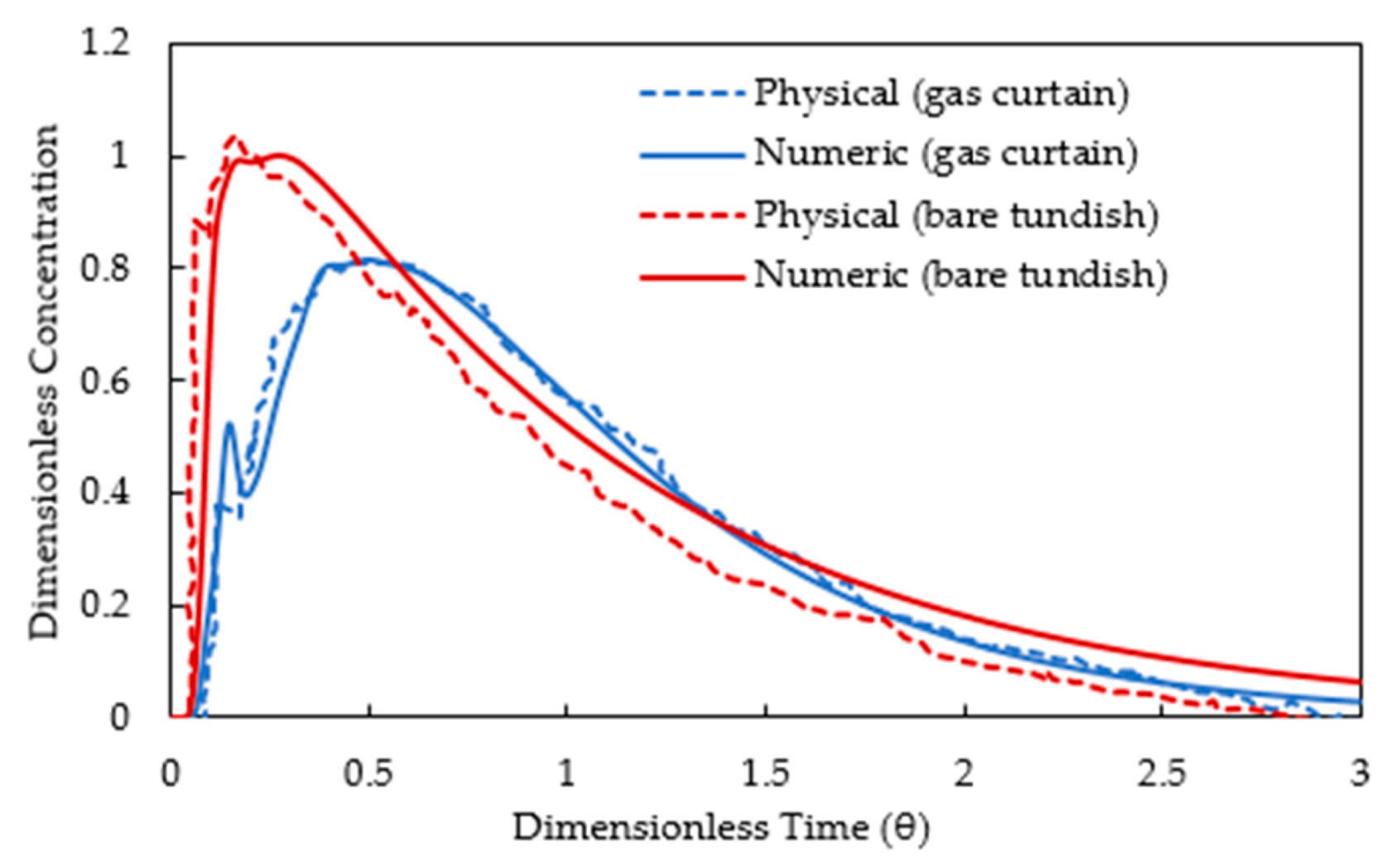
3.1. Validation of CFD Model

The CFD model was validated against the water model experiments reported in the literature by Chen et al. [34]. The geometrical scale of the water model is 1:2. The experiment was carried out with the dispersion of NaCl tracers. The pulse stimulus–response technique was employed to measure the RTD E-curves. The NaCl solution was infused through the tracer inlet in 2 s. The change of tracer concentration was registered continuously at the outlet.
The RTD curves calculated from the CFD model are shown in Figure 3 along with the water model results. The detailed input data for CFD calculations, including hydrodynamic parameters and material properties, can be found in [34]. Figure 3 shows that the peak time in the bare tundish (about 0.15 dimensionless time) was shorter than that in the gas curtain case (about 0.5 dimensionless time). This indicates that in the bare tundish most liquid flowed directly to the outlet, leading to a short residence time and large dead volume fraction. The gas curtain in tundish eliminated the short-circuit flow, increased the residence time, and decreased the dead volume fraction. There is good matching of the breakthrough time between the calculated and the measured results. The peak values also agreed well with the experiment. The slopes of E-curves after the peak were close to each other. Thus, the overall comparison between the simulation and the experiment is satisfactorily close.

3.2. CFD Simulation Results
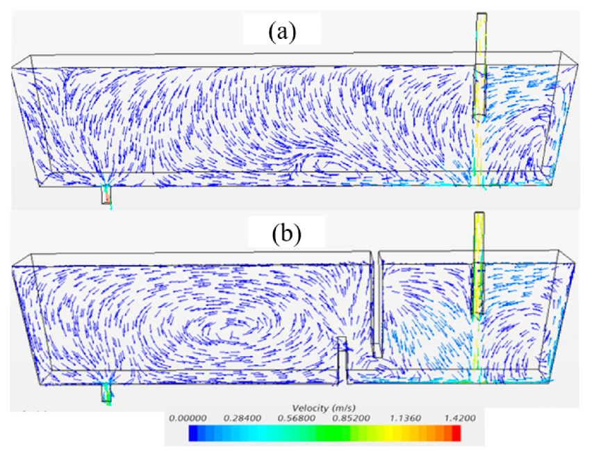
3.2.1. Fluid Flow

Figure 4 shows the predicted flow characteristics for Case 0 (bare tundish) and Case 1 (weir + dam). The entering liquid jet flows down to the bottom of the tundish and spreads rapidly in the right chamber. The flow is driven along the walls, then moves back to the entering jet. It forms counter flows near the inlet region. A part of the incoming stream is confined within the region near the inlet owing to the presence of the weir. Meanwhile, another part flow with high momentum moves underneath the weir and downstream towards the outlet direction.
The presence of a dam reorients the flow after the weir and drives the flow vertically towards the top surface. Thus, it increases the contact possibility between the inclusions and the top slag layer. In addition, the interference of the dam impairs the flow recirculation in the left chamber of the tundish, which improves the mixing of liquid steel. The configuration of Case 1 offers a higher plug volume fraction caused by the support of the weir and dam and also limits the extension of the turbulence zone. The horizontal velocities in the left chamber, predicted in Case 1, were higher compared with Case 0. This leads to an increase in mean residence time of liquid steel.

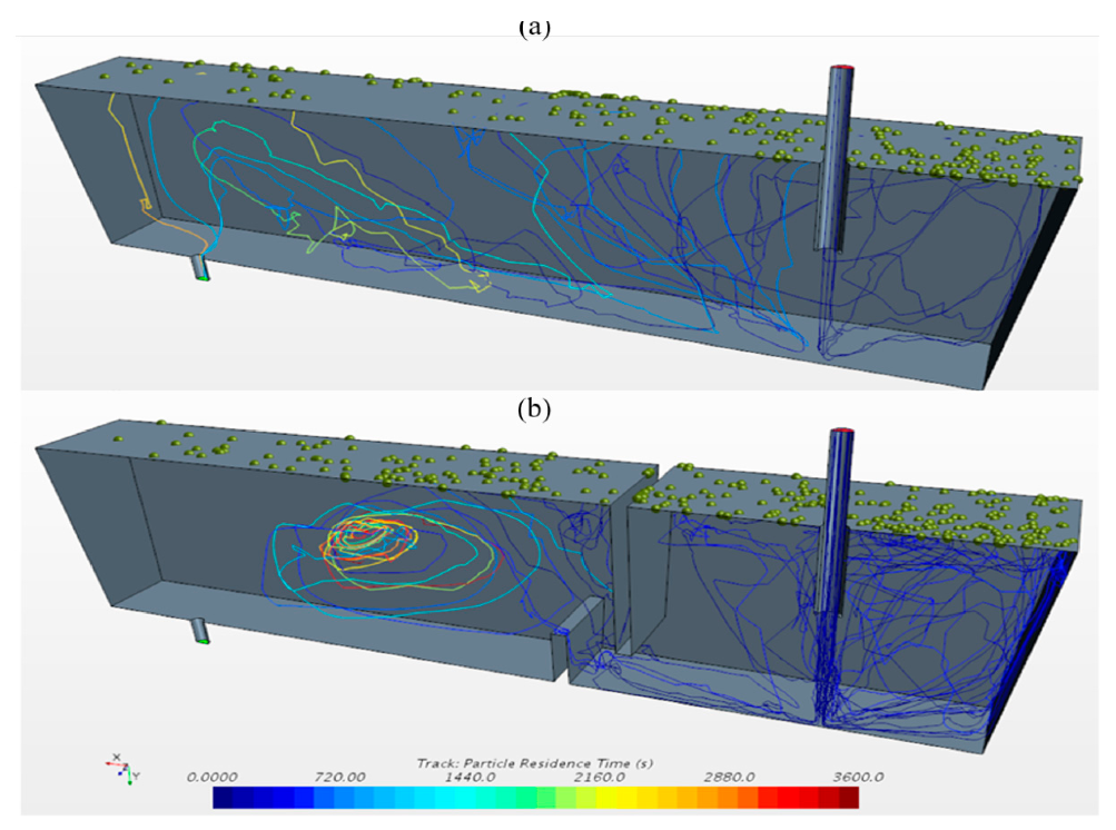
3.2.2. Inclusion Tracking

Figure 5 shows the representative trajectories of inclusions (density: 5000 kg·m−3, size: 50 μm) for the simulated Case 0 and Case 1. In the CFD model, inclusions are injected through the inlet plane. For better visibility, particle trajectories are colored by particle residence time. In Case 1, the existence of a weir and dam drives inclusions to a longer distance, resulting in a prolonged inclusion retention time. Most inclusions restricted by the weir were concentrated in the pouring area, indicating that the weir is conducive to the removal of inclusions in the pouring area. At the same time, the density of inclusion trajectories of the downstream area and the number of trajectories reaching the outlet in Case 1 were significantly lower than those in Case 0. It illustrates that the weir and dam could greatly improve the overall inclusion remove rate. The floating inclusions on the top surface of the tundish are presented in Figure 5. It shows that Case 1 had more entrapped particles at the top surface than Case 0.

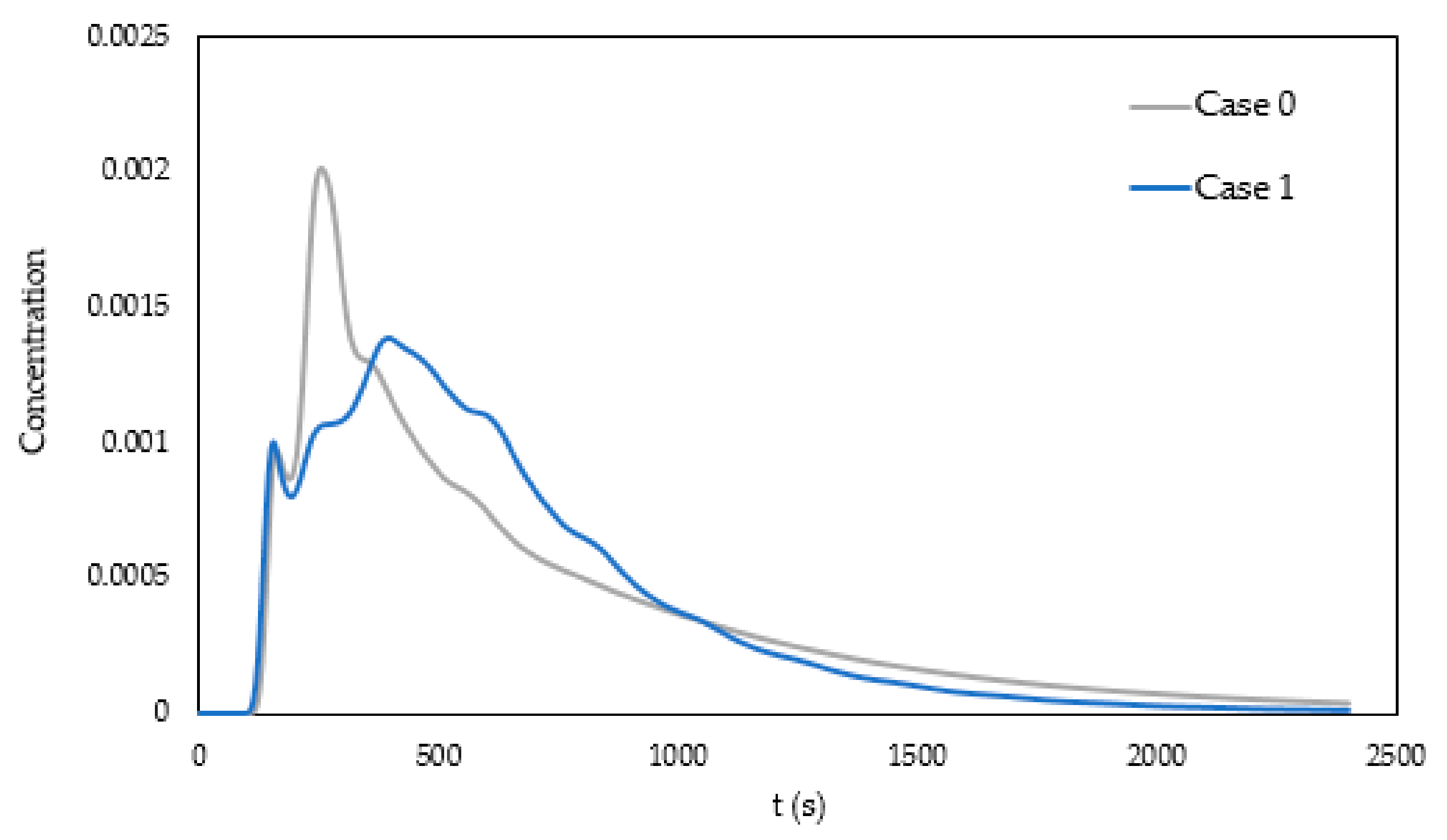
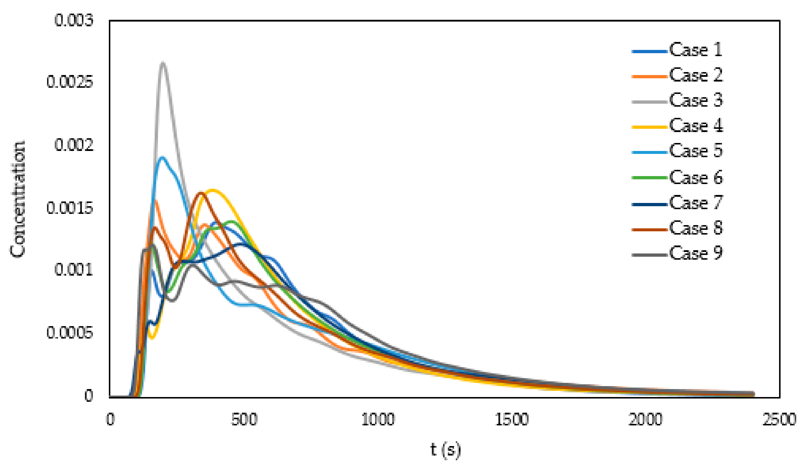
3.2.3. Residence-Time Distribution

The comparison of RTD curves between Case 1 and Case 0 is shown in Figure 6. For Case 0, bare tundish, the peak concentration was higher and the peak concentration time was shorter. This means more tracer left the tundish quickly after injection into the tundish. Such flow characteristics resulted in a large dead flow volume and short residence time. The RTD curve of Case 1 reveals a smoother curve, which means the flow characteristics in Case 1 were improved by using a weir and dam. The RTD curve in Case 0 has a long tail, indicating that a fraction of the fluid was retained in the dead zone for a very long time, causing the poor homogeneity of liquid steel in the tundish.

3.3. Optimization Analysis

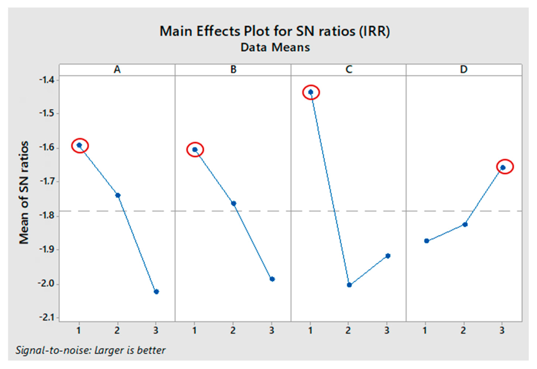
3.3.1. Single Response Optimization-Inclusion Remove Rate

The IRR values were calculated from the CFD particle tracking results, and their corresponding S/N ratios are listed in Table 5. The IRR values varied from 74.7% to 87.6%. The IRR response table for the design factors A, B, C, and D was created in the integrated manner, and the results are given in Table 6. Regardless of the category of the performance characteristics, a greater S/N value corresponds to a better performance. The design factors’ contribution order for IRR in the tundish process is C > A > B > D. From the analysis of the S/N ratio (Figure 7), the optimum levels of the design factors for IRR are determined as A1, B1, C1, and D3.
It should be mentioned here that the variation of IRR value is quite small, about 13% difference for the nine calculated cases. This is because the selected inclusion size was quite big (50 μm), and the inclusion floating velocity was high. From a practical point of view, it might be difficult to measure such a small difference in the real tundish process. As a first step of the method development, only one inclusion size was studied in order to reduce the complexity of the mathematical model. In future work, different inclusion sizes will be considered for the design purposes.
ANOVA was chosen to analyze the effects of various design factors on IRR. It comes with two merits: (1) obtaining contribution rate of design factors by analyzing the variation in factors, and (2) verifying the results’ reliability by Taguchi analysis. As listed in Table 7, the term DF represents the degree of freedom. The sequential (Seq SS) and adjusted (Adj SS) sums of squares indicate the relative importance of each factor. Adjusted mean squares (Adj MS) measure how much variation a term explains. The factor with the biggest coefficient and biggest sum of squares has the greatest impact.
To avoid zero degrees of freedom, factor D was set as a pooled factor in ANOVA due to its lowest significant influence, as shown in Table 6. The results of ANOVA in Table 7 indicate that factors A, B, and C influenced the IRR values by 24.64%, 19.18%, and 50.15%, respectively. The contribution rate of error was 6.03%, which comprises different error parts, such as the external sources and the calculation errors. The factor C (distance between weir and dam) had the highest percentile contribution on the inclusion removal rate. The significance of the design factors is determined as C > A > B, which is consistent with the results from the Taguchi method.

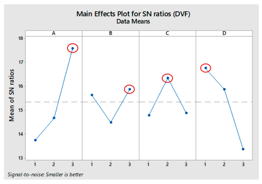
3.3.2. Single Response Optimization-Dead Volume Fraction

Nine CFD cases of the transient RTD simulations were performed based on the Taguchi L9(3^4) OA. Figure 8 and Table 8 show the predicted E-curve and RTD parameters. It was found that the selected design factors made a significant difference to the flow performance in the tundish, where the predicted dead volume fraction varied from 9% to 26%.
The DVF values calculated from the E-curves and their corresponding S/N ratio values are listed in Table 9. The IRR response table for factors A, B, C, and D were created in an integrated manner, and the results are given in Table 10. The optimal level of the DVF is the level with the greatest S/N value. The order of importance of the design factors to the DVF is A > D > C > B. From the analysis of the S/N ratio (Figure 9), the optimum levels of the design factors for DVF are determined as A3, B3, C2, and D1.
The results of ANOVA in Table 11 indicate that factors A, C and D influenced the DVF values by 45.82%, 7.52%, and 42.64%, respectively. The contribution rate of error was 4.02%. To avoid zero degrees of freedom in the ANOVA analysis, factor B was set as a pooled factor due to the lowest significant influence, as shown in Table 10. Factor A (distance between inlet and weir) had the highest percentile contribution on the dead volume fraction in the tundish. The significance of the design factors is determined as A > D > C, which is consistent with the results acquired from the Taguchi method.

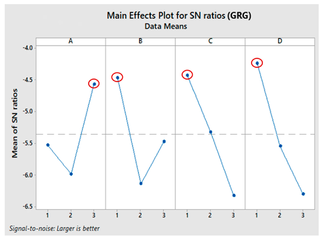
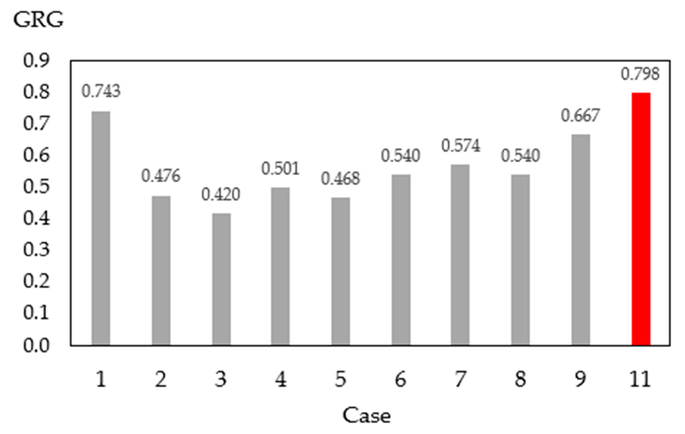
3.3.3. Multiple Response Optimization Using the Grey Relational Grade

Data pre-processing by GRA was performed on the CFD simulation results of the responses in Table 12, namely IRR and DVF. The multiple responses obtained were firstly normalized. Subsequently, the deviation sequences were computed. Then, the grey relational coefficient (GRC) for each value of the response was calculated. Finally, the average of the GRC was computed to determine the grey relational grade (GRG). The overall evaluation of the multiple performance characteristics was based on the GRG data. The grade with highest value was assigned the highest rank.
The GRG values and their corresponding S/N ratio values are listed in Table 13. The GRG response table for factors A, B, C, and D were created in an integrated manner, and the results are given in Table 14. The optimal level of the GRG is the level with the greatest S/N value. The order of importance of the design factors to the GRG in the tundish process is D > C > B > A. From the analysis of the S/N ratio of GRG (Figure 10), the optimum levels of the design factors are determined as A3, B1, C1, and D1.
As listed in Table 15, the results of ANOVA indicate that factors C, D, and B influenced the GRG by 26.13%, 36.48%, and 22.56%, respectively. Factor A was set as a pooled factor due to the lowest significant influence, as shown in Table 14. The contribution rate of error was 14.83%, which was quite large. This means that the pooled factor A had a relatively high contribution (shown in Figure 9). According to the ANOVA analysis, dam height had the highest percentile contribution on the DVF. The significance of the design factors is determined as D > C > B, which is consistent with the results acquired from the Taguchi method.

3.4. Confirmation Tests

The purpose of the confirmation tests was to validate the conclusion drawn during the analysis phase. A new CFD simulation case, Case 10, was created with the newest optimum levels of the design factors for inclusion removal rate; it is the combination of A1, B1, C1, and D3, as suggested in Section 3.3.1. According to the analysis from Section 3.3.2, the optimum levels of the control factors for DVF consisted of A3, B3, C2 and D1, which was exactly the same as Case 9 in the Taguchi L9(3^4) OA. In terms of gray relational grade, a new simulation case (Case 11) was created with the optimum levels of the control factors. It combines A3, B1, C1, and D1 in the design based on the analysis in Section 3.3.3.
Figure 11a gives the simulated IRR value of Case 10 and Case 11, as well as the nine cases from Taguchi L9(3^4) array described in Table 4. The inclusion removal of proposed optimum case (Case 10) was about 1% higher than that of Case 1 (87.6%), which had the highest inclusion removal in Taguchi OA. Furthermore, the simulated IRR (88.6%) of Case 10 was in good agreement with the predicted IRR value (89.4%) through DOE analysis, as shown in Table 16. Thus, the optimum case of IRR (Case 10) was verified. The suggested the optimum case of DVF from statistical analysis was also Case 9 from Taguchi OA. It had the best performance of dead volume fraction with 9.4%. It is interesting to observe that Case 9 showed the best performance in minimizing dead volume, but behaved worst in removing inclusion particles. This can infer that the two DVF and IRR responses in this study are in conflict with each other. It is therefore of importance to develop a design optimization process considering multiple responses simultaneously.
The proposed optimum case of GRG, Case 11, is a compromised design with the concern of two responses (IRR and DVF). Figure 12 gives the simulated GRG value of Case 11 together with the nine cases from Taguchi OA described in Table 4. Case 11 showed the highest gray relational grade with a value of 0.798. The design performance affirmed the validity of the Taguchi-GRA method for the multi-response optimization of IRR and DVF. A good conformity was obtained by comparing the simulated GRG value (0.798) by CFD and the predicted GRG value (0.79) by Taguchi-GRA, as shown in Table 16.

4. Summary and Conclusions

A novel digital design methodology that combined CFD simulation and Taguchi-Grey relational analysis was presented with the aim of optimizing the design of flow control devices (weir and dam) in a single-strand tundish. The design targets are set to maximize the inclusion removal rate and minimize the dead volume fraction in the tundish. Four design factors were selected, including distance between inlet and weir (A), distance of tundish bottom to weir (B), distance between weir and dam (C), and dam height (D). From the CFD simulation results and the DOE analysis, the main conclusions of this study can be drawn.
(1)
The fluid pattern and the residence-time distribution were improved in the tundish furnished with the weir and dam, in comparison with that in the bare tundish. The weir confined high turbulent flow in the entry zone and increased the inclusion removal possibility by the top surface. In addition, the dam drove the flow vertically towards the top surface and enhanced the inclusion removal.
(2)
With regard to the design optimization for the single response of IRR, the importance order of the design factors was concluded as C > A > B > D. The optimum levels of the control factors for IRR were determined as the combination of A1, B1, C1, and D3. The reliability of the Taguchi analysis results was verified by ANOVA.
(3)
In terms of single response of DVF, the importance order of the design factors was considered as A > D > C > B. The optimum levels of the control factors for DVF were predicted as the combination of A3, B3, C2, and D1. It was found that the optimum case of DVF had the best performance in minimizing dead volume, but the worst performance in removing inclusion particles. The conflicting responses suggests the necessity of developing a compromised optimization process of multiple objectives. The evaluation of the multiple responses was based on the grey relational grade. The importance order of the design factors for GRG is termed as D > C > B > A. The dam height was the most important factor affecting the GRG. The optimum levels of the control factors were termed as the mixture of A3, B1, C1, and D1.
(4)
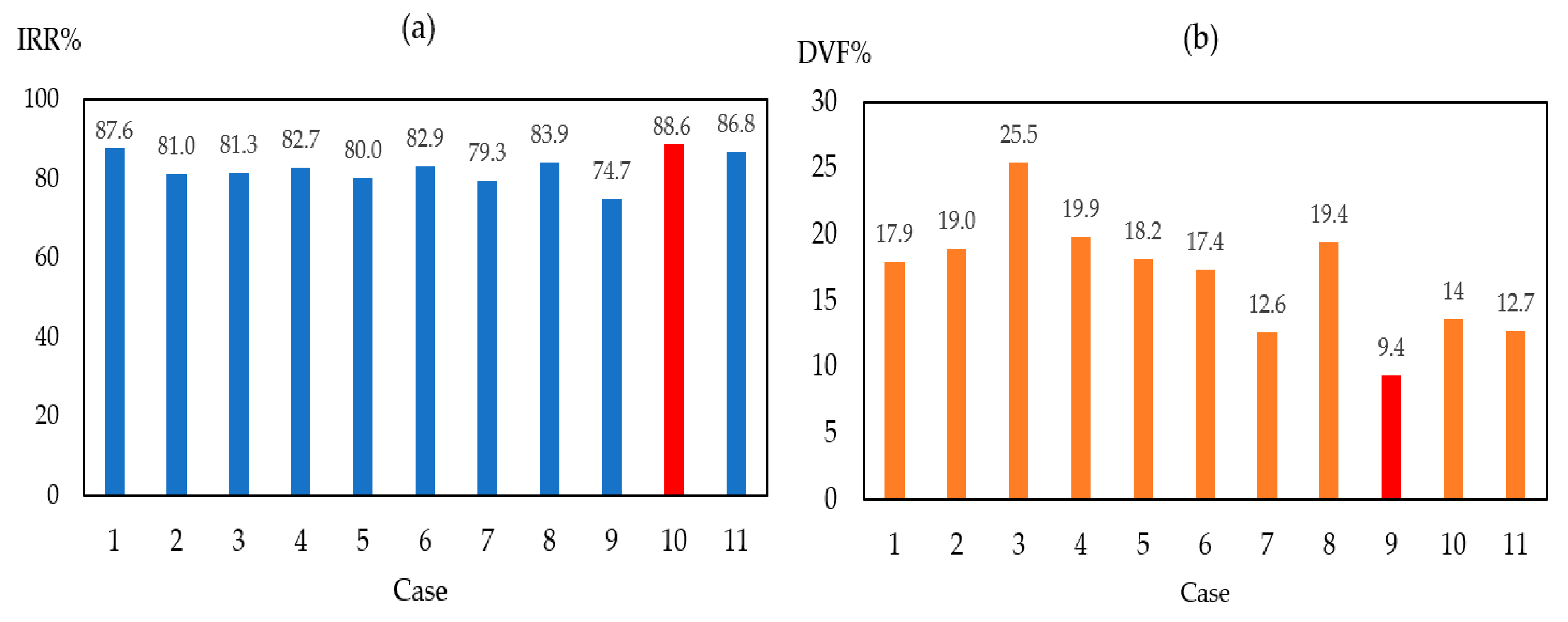
The confirmation tests with regards to the different responses (IRR, DVF, and GRG) were performed. The optimum results from CFD simulations revealed the increased performance of the responses. An excellent agreement was observed between the CFD simulations and the DOE predictions.
(5)
The present study demonstrated that the application of CFD combined with the Taguchi-GRA method was effective in finding the optimal design that improved the tundish performance. The developed method may provide both time and cost savings not only for researchers but also for the steel industry. As shown in this study, a full design space (four design factors and three levels) requires a total of 81 (3 × 3 × 3 × 3) computer runs. By applying the Taguchi orthogonal arrays method, the computer runs can be significantly reduced to 9. Furthermore, the conclusions drawn from small-scale experiments are valid over the entire experimental region spanned by the design factors and their levels. Future work should test the applicability of the developed design methodology in a wider range of experiment conditions.

Funding

This paper was supported by the Swedish Foundation for Strategic Research (SSF)—Strategic Mobility Program (2019).

Acknowledgments

The author would like to acknowledge the Swedish Foundation for Strategic Research (SSF) for their financial support via Strategic Mobility Program (2019).

Conflicts of Interest

The author declares no conflict of interest.

Nomenclature

Adj SSAdjusted sums of squares
Adj MSAdjusted mean squares
DeffEffective diffusivity
FdDrag force
FpPressure gradient force
FvmVirtual mass forces
FgGravitational force
FlLift force
FtdTurbulent dispersion
gGravity
GkTurbulent kinetic energy
kTurbulent kinetic energy
miMass
nobservation repeat number
SFSource term
s2the variance
Seq SSSequential sums of squares
uVelocity of the flow field
vlThe velocity of liquid
vpThe velocity of particle
VpVelocity of particle i
υKinematic viscosity
xi(k)sequence for the ith experiment
x0(k)reference sequence
yperformance characteristic value
ξ Grey relational coefficient
µMolecular viscosity
µtTurbulent viscosity
ρDensity
w(k)weight factor of the number k influence
Δdeviation

Abbreviations

ANOVAAnalysis of Variance
CCContinuous Casting
CADComputational Aided Design
CFDComputational Fluid Dynamics
DOEDesign of Experiment
DVFDead Volume Fraction
FCDFlow Control Device
GRAGrey Relational Analysis
GRCGrey Relational Coefficient
GRGGrey Relational Grade
IRRInclusion Removal Rate
OAOrthogonal Array
RTDResidence-time distribution
S/NSignal-to-noise ratio
MSTmean square for treatments
MSEmean square for error

References

  1. Szekely, J.; Ilegbusi, O.J. The Physical and Mathematical Modeling of Tundish Operations; Springer Science and Business Media LLC: New York, NY, USA, 1989. [Google Scholar]
  2. Mazumdar, D.; Guthrie, R.I.L. The Physical and Mathematical Modelling of Continuous Casting Tundish System. ISIJ Int. 1999, 39, 524–547. [Google Scholar] [CrossRef]
  3. Chattopadhyay, K.; Isac, M.; Guthrie, R.I.L. Physical and Mathematical Modelling of Steelmaking Tundish Operations: A Review of the Last Decade (1999–2009). ISIJ Int. 2010, 50, 331–348. [Google Scholar] [CrossRef] [Green Version]
  4. Mazumdar, D. Review, Analysis, and Modeling of Continuous Casting Tundish Systems. Steel Res. Int. 2019, 90, 1800279. [Google Scholar] [CrossRef]
  5. Sheng, D.-Y.; Yue, Q. Modeling of Fluid Flow and Residence-Time Distribution in a Five-strand Tundish. Metals 2020, 10, 1084. [Google Scholar] [CrossRef]
  6. Sheng, D.-Y. Mathematical Modelling of Multiphase Flow and Inclusion Behavior in a Single-Strand Tundish. Metals 2020, 10, 1213. [Google Scholar] [CrossRef]
  7. Taguchi, G.; Chowdhury, S.; Wu, Y. Taguchi’s Quality Engineering Handbook; John Wiley & Sons Inc.: Hoboken, NJ, USA, 2005. [Google Scholar]
  8. Taguchi, G. Off-line and On-line Quality Control Systems. In Proceedings of the International Conference on Quality Control, Tokyo, Japan, 17–20 October 1978. [Google Scholar]
  9. Joo, S.; Han, J.W.; Guthrie, R.I.L. Inclusion behavior and heat-transfer phenomena in steelmaking tundish operations: Part III. applications—Computational approach to tundish design. Met. Mater. Trans. A 1993, 24, 779–788. [Google Scholar] [CrossRef]
  10. Craig, K.J.; De Kock, D.J.; Makgata, K.W.; De Wet, G.J. Mathematical Modeling of Iron and Steel Making Processes. Design Optimization of a Single-strand Continuous Caster Tundish Using Residence Time Distribution Data. ISIJ Int. 2001, 41, 1194–1200. [Google Scholar] [CrossRef]
  11. Jha, P.K.; Dash, S.K. Employment of different turbulence models to the design of optimum steel flows in a tundish. Int. J. Numer. Methods Heat Fluid Flow 2004, 14, 953–979. [Google Scholar] [CrossRef]
  12. Hülstrung, J.; Zeimes, M.; Au, A.; Oppermann, W.; Radusch, G. Optimization of the Tundish Design to Increase the Product Quality by means of Numerical Fluid Dynamics. Steel Res. Int. 2005, 76, 59–63. [Google Scholar] [CrossRef]
  13. Wei, Z.; Bao, Y.; Liu, J.; Gong, W.; Wang, B. Orthogonal analysis of water model study on the optimization of flow control devices in a six-strand tundish. J. Univ. Sci. Technol. Beijing Miner. Met. Mater. 2007, 14, 118–124. [Google Scholar] [CrossRef]
  14. Kumar, A.; Mazumdar, D.; Koria, S.C. Modeling of Fluid Flow and Residence Time Distribution in a Four-strand Tundish for Enhancing Inclusion Removal. ISIJ Int. 2008, 48, 38–47. [Google Scholar] [CrossRef] [Green Version]
  15. Singh, V.; Pal, A.R.; Panigrahi, P. Numerical Simulation of Flow-induced Wall Shear Stress to Study a Curved Shape Billet Caster Tundish Design. ISIJ Int. 2008, 48, 430–437. [Google Scholar] [CrossRef] [Green Version]
  16. Yang, S.; Zhang, L.; Li, J.; Peaslee, K. Structure Optimization of Horizontal Continuous Casting Tundishes Using Mathematical Modeling and Water Modeling. ISIJ Int. 2009, 49, 1551–1560. [Google Scholar] [CrossRef] [Green Version]
  17. Cwudziñski, A. Numerical Simulation of Liquid Steel Flow in Wedge-type One-strand Slab Tundish with a Subflux Turbulence Controller and an Argon Injection System. Steel Res. Int. 2010, 81, 123–131. [Google Scholar] [CrossRef]
  18. Tripathi, A. Numerical Investigation of Electro-magnetic Flow Control Phenomenon in a Tundish. ISIJ Int. 2012, 52, 447–456. [Google Scholar] [CrossRef] [Green Version]
  19. Shukla, R.; Anapagaddi, R.; Mangal, S.; Singh, A.K. Exploring the Design Space of a Continuous Casting Tundish for Improved Inclusion Removal and Reduced Dead Volume. In Proceedings of the Science and Technology of Ironmaking and Steelmaking, Jamshedpur, India, 16–18 December 2013. [Google Scholar]
  20. Anapagaddi, R.; Shukla, R.; Goyal, S.; Singh, A. Exploration of the Design Space in Continuous Casting Tundish. In Proceedings of the ASME 2014 International Design Engineering Technical Conference, New York, NY, USA, 17–20 August 2014. [Google Scholar]
  21. Cloete, J.; Akdogan, G.; Bradshaw, S.; Chibwe, D. Physical and numerical modelling of a four-strand steelmaking tundish using flow analysis of different configurations. J. S. Afr. Inst. Min. Met. 2015, 115, 355–362. [Google Scholar] [CrossRef]
  22. He, F.; Zhang, L.-Y.; Xu, Q.-Y. Optimization of flow control devices for a T-type five-strand billet caster tundish: Water modeling and numerical simulation. China Foundry 2016, 13, 166–175. [Google Scholar] [CrossRef]
  23. Buľko, B.; Priesol, I.; Demeter, P.; Gašparovič, P.; Baricová, D.; Hrubovčáková, M. Geometric Modification of the Tundish Impact Point. Metals 2018, 8, 944. [Google Scholar] [CrossRef] [Green Version]
  24. Rocha, J.R.D.S.; De Souza, E.E.B.; Marcondes, F.; De Castro, J.A. Modeling and computational simulation of fluid flow, heat transfer and inclusions trajectories in a tundish of a steel continuous casting machine. J. Mater. Res. Technol. 2019, 8, 4209–4220. [Google Scholar] [CrossRef]
  25. Anthony, J. Design of Experiments for Engineers and Scientists; Elsevier: Amsterdam, The Netherlands, 2003. [Google Scholar]
  26. Minitab 18 Statistical Software; Minitab, Inc.: State College, PA, USA, 2017. Available online: www.minitab.com (accessed on 7 June 2017).
  27. Fisher, R.A. Statistical Methods for Research Workers; Oliver & Boyd: Edinburgh, UK, 1925. [Google Scholar]
  28. Deng, J.-L. Control Problems of Grey Systems. Syst. Control Lett. 1982, 1, 288–294. [Google Scholar]
  29. Wikipedia. Available online: https://en.wikipedia.org/wiki/Grey_relational_analysis (accessed on 27 June 2020).
  30. Yin, M.-S. Fifteen years of grey system theory research: A historical review and bibliometric analysis. Expert Syst. Appl. 2013, 40, 2767–2775. [Google Scholar] [CrossRef]
  31. Siemens. STAR-CCM + Version 13.04 User Guide; Siemens PLM Software: Munich, Germany, 2019. [Google Scholar]
  32. Ghirelli, F.; Hermansson, S.; Thunman, H.; Leckner, B. Reactor residence time analysis with CFD. Prog. Comput. Fluid Dyn. Int. J. 2006, 6, 241. [Google Scholar] [CrossRef]
  33. Spalding, D. A note on mean residence-times in steady flows of arbitrary complexity. Chem. Eng. Sci. 1958, 9, 74–77. [Google Scholar] [CrossRef]
  34. Chen, D.; Xie, X.; Long, M.; Zhang, M.; Zhang, L.; Liao, Q. Hydraulics and Mathematics Simulation on the Weir and Gas Curtain in Tundish of Ultrathick Slab Continuous Casting. Met. Mater. Trans. A 2013, 45, 392–398. [Google Scholar] [CrossRef]
Figure 1. Dimensions of a single-strand tundish: (a) side view (b) front view (unit: mm). Design factors: A (distance between inlet and weir); B (distance of tundish bottom to weir); C (distance between weir and dam); D (dam height).
Metals 10 01539 g001
Figure 2. Flow diagram of design process to optimize flow control device in tundish.
Metals 10 01539 g002
Figure 3. RTD curves of physical modelling and numerical modelling results (bare tundish and tundish with gas curtain).
Metals 10 01539 g003
Figure 4. Velocity vectors at the center longitudinal plane: (a) Case 0, bare tundish; (b) Case 1, weir + dam.
Metals 10 01539 g004
Figure 5. Representative trajectories of inclusions in the tundish: (a) Case 0, bare tundish; (b) Case 1, weir + dam (inclusion density: 5000 kg·m−3, size: 50 μm).
Metals 10 01539 g005
Figure 6. Comparison of RTD curves between Case 1 and Case 0 (Case 0, bare tundish; Case 1, weir + dam).
Metals 10 01539 g006
Figure 7. Mean of S/N ratio (IRR) for each factor at levels 1–3.
Metals 10 01539 g007
Figure 8. RTD curves of nine simulated cases based on Taguchi L9(3^4) OA.
Metals 10 01539 g008
Figure 9. Mean of S/N ratio (DVF) for each factor at levels 1–3.
Metals 10 01539 g009
Figure 10. Mean of S/N ratio (GRG) for each factor at levels 1-3.
Metals 10 01539 g010
Figure 11. Simulated IRR and DVF values by CFD: (a) IRR; (b) DVF.
Metals 10 01539 g011
Figure 12. Simulated GRG values by CFD.
Metals 10 01539 g012
Table 1. Summary of investigations modelling the optimum tundish design.
ReferenceCodeStudy 1Strand 1Turb. 2Tundish Design
CaseMethod 3FCD 4Design Factors 5Perform. Feature 6
Joo (1993) [9]METFLOn2k − ε13-D, WSFR, WAI, CFCD, WL, DL,FP, IRR
Craig (2001) [10]FLUENTn1k − ε20RSMTI, B, D, W, SWL, DL BL, BHA, FTFP, RTD
Jha(2004) [11]-N6(vari.)6-TITM, OL, TIH, IDRTD
Hülstrung (2005) [12]-N2k − ε10-S, TISFR, ID, IFR, CFCDV, IRR, RTD
Wei (2007) [13]-P6-25TaguchiBBD, HLRTD
Kumar (2008) [14]FLUENTN/P2–6k − ε3-D, TICFCDV, RTD
Singh (2008) [15]FLUENTN/P6k − ε6-TIWAC, WAIA, TWV, WSS, RTD
Yang (2009) [16]FLUENTN/P/I2k − ε5-TI, IL, B, DDH, ILTFP, RTD, V, WSS, T, IRR, TO, TN
Cwudziński (2010) [17]FLUENTN/I1k − ε12-S, TI, D, GPBCFCD, GPBL, GFRFP, RTD
Tripathi (2012) [18]FLUENTN1k − ε9-EDEDL, MSV, RTD
Shukla (2013) [19]CFXN/P1k − ε-TaguchiD, WDH, DT, DL, WD, WT, WL, SFRRTD, IRR
Anapagaddi (2014) [20]CFXN1k − ε7RSMD, WIT, SFR, WL, WD, WT, DL, DH, DTRTD, IRR
Cloete (2015) [21]FLUENTN/P4k − ε4-TI, DCFCD, TIS, DHV, KE, RTD
He (2016) [22]FLUENTN/P5k − ε3-TI, BCFCDFS, V, T
Buľko (2018) [23]FLUENTN/P2k − ε6-TITIS, SFRRTD, V
Sousa Rocha (2019) [24]CFXN/P2k − ε/SST3-D, WCFCD, IDRTD, IRR, FP, T
1N: numerical model; P: physical model; I: industrial trials; 2 Turb.: turbulence model; vari.: turbulence model as variables; 3 Method.: Optimization or design method; RSM: response surface models; 4 FCD: flow control devices; B: baffle; D: dam; ED: electromagnetic dam; GPB: gas permeable barrier; IL: inlet lauder; S: stopper; TI: turbulence inhibitor; W: weir; 5 BD: bath depth; BL: baffle location; BHA: baffle hole angle; CFCD: combination of flow control devices; DL: dam location; DH: dam height; DT: dam thickness; EDL: electromagnetic dam location; FT: fluid type; HL: hole location; IT: inlet temperature; ID: inlet depth; ILT: inlet lauder type; ID: inclusion diameter; IFR: inclusion flow rate; GPBL: gas permeable barrier location; GFR: gas flow rate; MS: magnetic strength; OL: outlet location; SFR: steel flow rate; TM: Turbulence Model; TW: tundish width; TIS: turbulence inhibitor shape; TIH: turbulence inhibitor height; WL: weir location; WD: weir depth; WT: weir thickness; WAC: wall curvature; WAI: wall inclination; WAIA: wall inclination angle; 6 Perform. Feature: performance feature; FS: flow streamline; FP: flow pattern; IRR: inclusion removal rate; KE: kinetic energy RTD: residence time distribution parameter; T: temperature; TO: total oxygen measurement in steel sample; TN: total nitrogen measurement in steel sample; V: velocity; WSS: wall shear stress.
Table 2. Controlled factors and levels.
FactorUnitLevel 1Level 2Level 3
Amm6408401040
Bmm180230280
Cmm230430630
Dmm220280340
Table 3. Orthogonal array L9(3^4).
CaseABCD
Case 0----
Case 11111
Case 21222
Case 31333
Case 42123
Case 52231
Case 62312
Case 73132
Case 83213
Case 93321
Table 4. Parameters and boundary conditions used for CFD simulations.
ParameterValue
Inlet velocity1 m/s
Steel density7020 kg/m3
Steel viscosity0.006 Pa s
Reference pressure101325 Pa
Inclusion velocity1 m/s
Inclusion size50 μm
Inclusion density5000 kg/m3
Outlet (outflow ratio)1
WallNo slip
Top surfaceFree slip
Tracer inlet (E-curve)1 (t ≤ 0–2 s), 0 (t > 2 s)
Table 5. Taguchi L9(3^4) OA and single response results (IRR) with signal-to-noise (S/N) ratios.
CaseABCDIRRS/N
111110.876−1.15
212220.81−1.83
313330.813−1.8
421230.827−1.65
522310.8−1.94
623120.829−1.63
731320.793−2.01
832130.839−1.52
933210.747−2.53
Table 6. Response table for signal-to-noise ratios of IRR.
LevelABCD
1−1.593−1.605−1.435−1.874
2−1.739−1.764−2005−1.825
3−2.024−1.987−1.917−1.658
Delta0.4310.3820.5700.216
Rank2314
Table 7. ANOVA table for inclusion removal rate.
SourceDFSeq SSContributionAdj SSAdj MSF-Value
A20.00246424.64%0.0024640.0012324.09
B20.00191819.18%0.0019180.0009593.18
C20.00501450.15%0.0050140.0025078.32
Error20.0006036.03%0.0006030.000301-
Total80.009999100.00%---
Table 8. RTD analysis of nine simulated cases.
Casettheo (s)tmin (s)tmax (s)tmean (s)Vd/V %Vp/V %Vm/V %
Case 0742100251629152461
Case 1729365396599185230
Case 272992165591191863
Case 372999197543262054
Case 472995382584203347
Case 5729103195597182061
Case 6729224452603174636
Case 772976485637133849
Case 8729134338588193248
Case 97298315766191674
Table 9. Taguchi L9(3^4) OA and S/N ratio of DVF (single response).
CaseABCDDVFS/N
111110.17914.933
212220.19014.447
313330.25511.869
421230.19914.033
522310.18214.796
623120.17415.195
731320.12617.966
832130.19414.230
933210.09420.579
Table 10. Response table for S/N ratios of DVF.
LevelABCD
113.7515.6414.7916.77
214.6714.4916.3515.87
317.5915.8814.8813.38
Delta3.841.391.573.39
Rank1432
Table 11. ANOVA table for dead volume fraction.
SourceDFSeq SSContributionAdj SSAdj MSF-Value
A20.00759745.82%0.0075970.00379811.39
C20.0012477.52%0.0012470.0006231.87
D20.00707042.64%0.0070700.00353510.60
Error20.0006674.02%0.0006670.000333-
Total80.016580100.00%---
Table 12. Data processing of grey relational analysis.
CaseABCDIRRDVFNormalizationDeviation SequenceGray Relational CoefficientGRGRank
IRRDVFIRRDVFIRRDVF
1111187.6181.0000.4690.0000.5311.0000.4850.7431
2122281.0190.4880.4060.5120.5940.4940.4570.4767
3133381.3260.5120.0000.4881.0000.5060.3330.4209
4212382.7200.6200.3480.3800.6520.5680.4340.5016
5223180.0180.4110.4520.5890.5480.4590.4770.4688
6231282.9170.6360.5020.3640.4980.5780.5010.5405
7313279.3130.3570.7970.6430.2030.4370.7110.5743
8321383.9190.7130.3760.2870.6240.6350.4450.5404
9332174.790.0001.0001.0000.0000.3331.0000.6672
Table 13. Taguchi L9(3^4) OA and S/N ratio of GRG (multiple responses).
CaseABCDGRGS/N
111110.743−2.585
212220.476−6.456
313330.420−7.543
421230.501−5.999
522310.468−6.594
623120.540−5.355
731320.574−4.821
832130.540−5.350
933210.667−3.522
Table 14. Response table for S/N ratios of GRG.
LevelABCD
1−5.528−4.468−4.430−4.234
2−5.983−6.133−5.326−5.544
3−4.564−5.473−6.319−6.297
Delta1.4191.6651.8902.064
Rank4321
Table 15. ANOVA table for grey relational grade.
SourceDFSeq SSContributionAdj SSAdj MSF-Value
C20.0217126.13%0.021710.0108531.76
D20.0303036.48%0.030300.0151502.46
B20.0187422.56%0.018740.0093721.52
Error20.0123214.83%0.012320.006160-
Total80.08307100.00%---
Table 16. Results of confirmation tests.
ResponseDesignCaseCFDPrediction
IRRA1B1C1D31088.6%89.4%
DVFA3B3C2D199.4%9.35%
GRGA3B1C1D1110.7980.790
Case 11- IRR: 86.8%; and DVF: 12.7% (CFD calculated)
Publisher’s Note: MDPI stays neutral with regard to jurisdictional claims in published maps and institutional affiliations.

