Analysis of Modified Finite Length Journal Bearing under Position Perturbation

Abstract

The performance of journal bearings is significantly affected by the presence of misalignment, which is usually an accompanying problem for this type of bearing. This includes exceeding the design limits for the maximum pressure and the minimum film thickness levels, which affect, in other words, the load-carrying capacity of the system. In addition, it raises the possibility of increasing the wear rate at the bearing edges and increases the friction coefficient at high levels of misalignment. This paper deals with the problem of finite-length misaligned journal bearings, considering a novel comparison between two cases of misalignments: the general 3D misalignment and the vertical misalignment problems for modified bearings. The effect of introducing a variable axial bearing profile on the bearing characteristics and the time responses of the rotor bearing system under position perturbation has also been investigated. The numerical solution of this hydrodynamic problem is based on the finite difference method using Reynolds boundary conditions method. Results show that using a variable bearing profile improves bearing characteristics, such as increasing the minimum film thickness significantly and reducing the pressure levels in addition to reducing the friction coefficient. Furthermore, the modification enhances the rotor-bearing stability under position perturbation, extending the speed range for a safe operation.

1. Introduction

The generation of hydrodynamic pressure, or the load-carrying capacity, results from the squeeze motion or the relative sliding between surfaces separated by a thin layer of lubricant. This is the basic concept of the hydrodynamic lubrication regime in journal bearings, the most common type of bearing in industrial applications. Such applications include supporting the rotating shaft in a wide range of machines, such as internal combustion engines, turbo-generators, compressors, pumps, etc. [1]. Despite the well design of the journal bearings used in these high-speed rotating machineries, the shaft supported by this type of bearing usually operates under a misalignment condition [2].

In an ideal situation, which rarely exists, the shaft and bush axes are always parallel. However, as the load and speed are imposed, the shaft will be subjected to misalignment while rotating inside its bearing [1]. One of the main negative effects of the misalignment is the considerable reduction in the levels of lubricant layer thickness. The designed minimum film thickness is responsible for preventing any direct contact between the journal and the bush surfaces, which is clearly affected by the presence of misalignment. Therefore, as the misalignment actually has a serious impact on the performance and life span of the journal bearing, this subject has drawn the attention of researchers over the last decades. Singh and Sinhasan [3], for example, investigated the consequences of small misalignment on the dynamic characteristics of big end bearing using the finite element method. Their result showed that the misalignment reduces the minimum film thickness by 28% in comparison with the perfectly aligned bearing. Choy et al. studied the nonlinear behavior of the dynamic coefficients. Choy et al. [4] analyzed the nonlinear behavior of the stiffness and damping coefficients of a journal bearing considering the misalignment effect using the finite difference method. Nikolakopoulos and Papadopoulos [5] analyzed the problem of a misaligned journal using the finite element method in order to solve the Reynolds equation. They calculated the linear and nonlinear dynamic characteristics for the misaligned bearing based on the fluid forces and moments, which were the function of the displacements and the angle of misalignment.

The dynamic characteristics of the journal bearing were studied by Ebrat et al. [6], considering misalignment effects. Their results showed that it is necessary to take the shaft misalignment into consideration when assessing the dynamic behavior of the rotor-bearing system. The misalignment in the journal bearing was also shown by Sun and Gui [7], Jang and Khonsari [1], and Jamali and Al-Hamood [8] to have a significant negative consequence on the general performance of the bearing system. Recently, Song et al. [9] explained that misalignment causes an obvious increase in friction over the mixed lubrication region. The friction (and wear) problems in this type of bearing have also drawn the researcher’s attention due to its effects on the bearing life and the system’s general performance.

Dufrane et al. [10] suggested a model for studying the wear effect on hydrodynamic lubrication performance. Their results showed an important outcome, which related an optimum film thickness value to the rate of wear progress in bearings. Bouyer and Fillon [11] conducted a very important experimental study to consider the misalignment effect on journal-bearing performance. They found that the performance of the bearing is significantly affected by the presence of misalignment, such as the 80% reduction in the minimum value of the film thickness. Sun et al. [12] showed that the misalignment changes the distributions and the values of the pressure field as well as the film thickness when they used a special test bench in their experimental study. Padelis et al. [13] used a numerical solution in order to determine the relationship among wear depth, coefficient of friction, and misalignment in journal bearings, where they suggested that functions relate these parameters.

Despite the usual unavoidable presence of misalignment in the journal bearing, it is possible to some extent to limit its negative effects on the system performance. The improvement of the bearing characteristics in terms of bearing geometry optimization was studied experimentally by Nacy [14], where he chamfered the edges of the bearing in an attempt to reduce the lubricant side leakage. Modifying the bearing geometry was also performed by Bouyer and Fillon [15], where they used predesigned defects in order to evaluate the bearing characteristics under misalignment. Strzelecki [16] used variable bearing profiles over the whole bearing width, where his results showed that such modifications help carry a high load despite misalignment. Chasalevris and Dohnal [17] used variable geometry for the journal bearing to enhance the dynamic behavior of the system. Recently Ren at al. [18] investigated the effects of profile parameters on the performance of the bearing where they explained that using quadratic profile improves the bearing characteristics. Jamali et al. [19,20] investigated the dynamic behavior of misaligned bearings. Allmaier and Offner [21] reviewed the simulation of journal bearings considering the elastohydrodynamic regime. They considered several topics, such as mixed lubrication, low-viscosity lubricant, and polymer coatings. This review emphasized that journal bearings are still facing new challenges, which motivate the researcher to develop more accurate and new methods to address the previously mentioned topics.

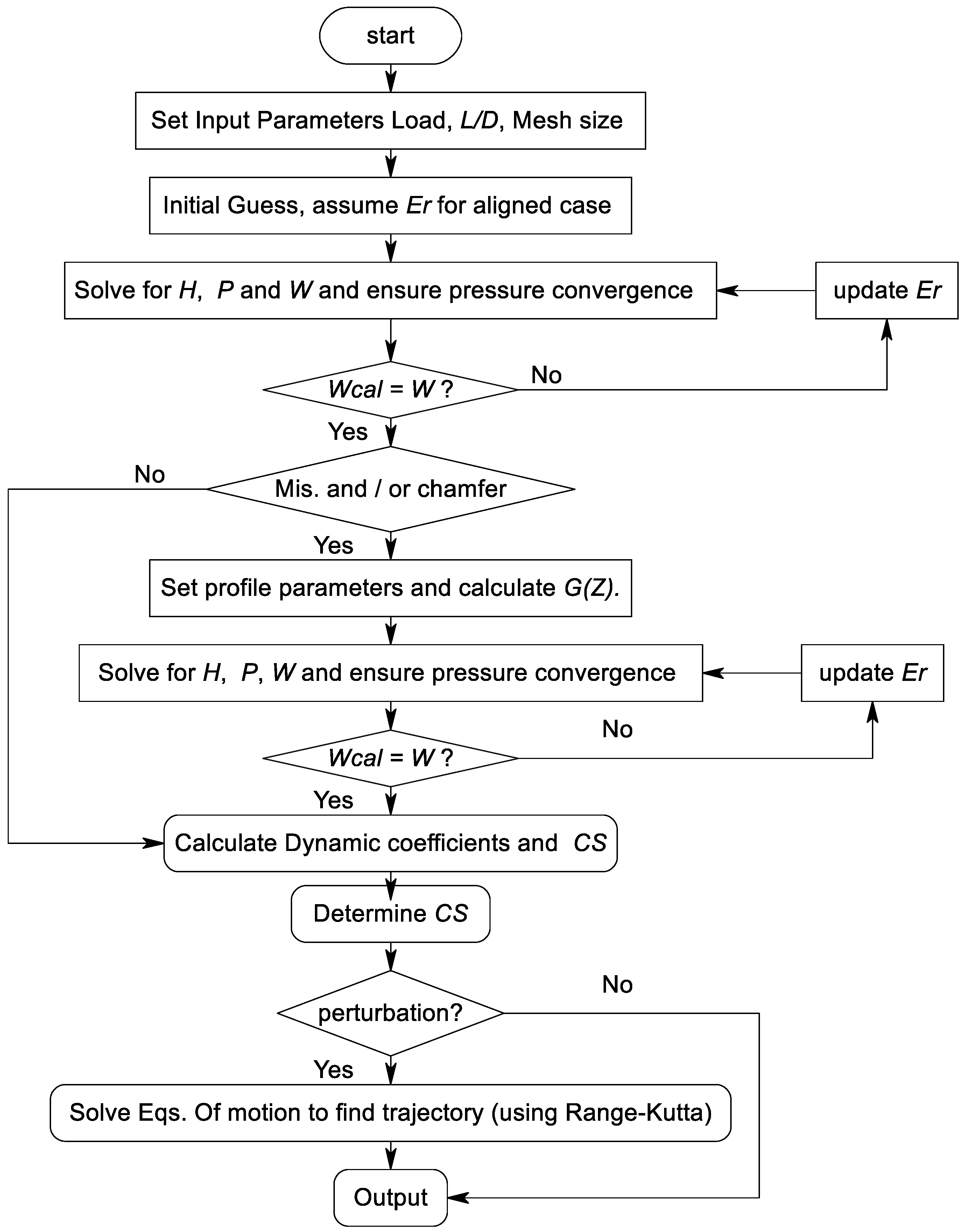
This paper presents a novel comparison between the misalignment in the vertical plain and the general 3D misalignment case for modified bearings. The numerical solution for the problem of hydrodynamic journal bearing is based on the finite difference method, and the Reynolds boundary condition method is followed to identify the boundaries of the cavitation zone. The variable bearing profile is considered in the analysis in order to reduce the misalignment effect on the friction coefficient, film thickness, and pressure distribution. Furthermore, the effects of varying bearing profiles on the time responses of the system to position perturbation of the journal as well as the stability threshold, are also investigated.

2. The General Model of the Solution

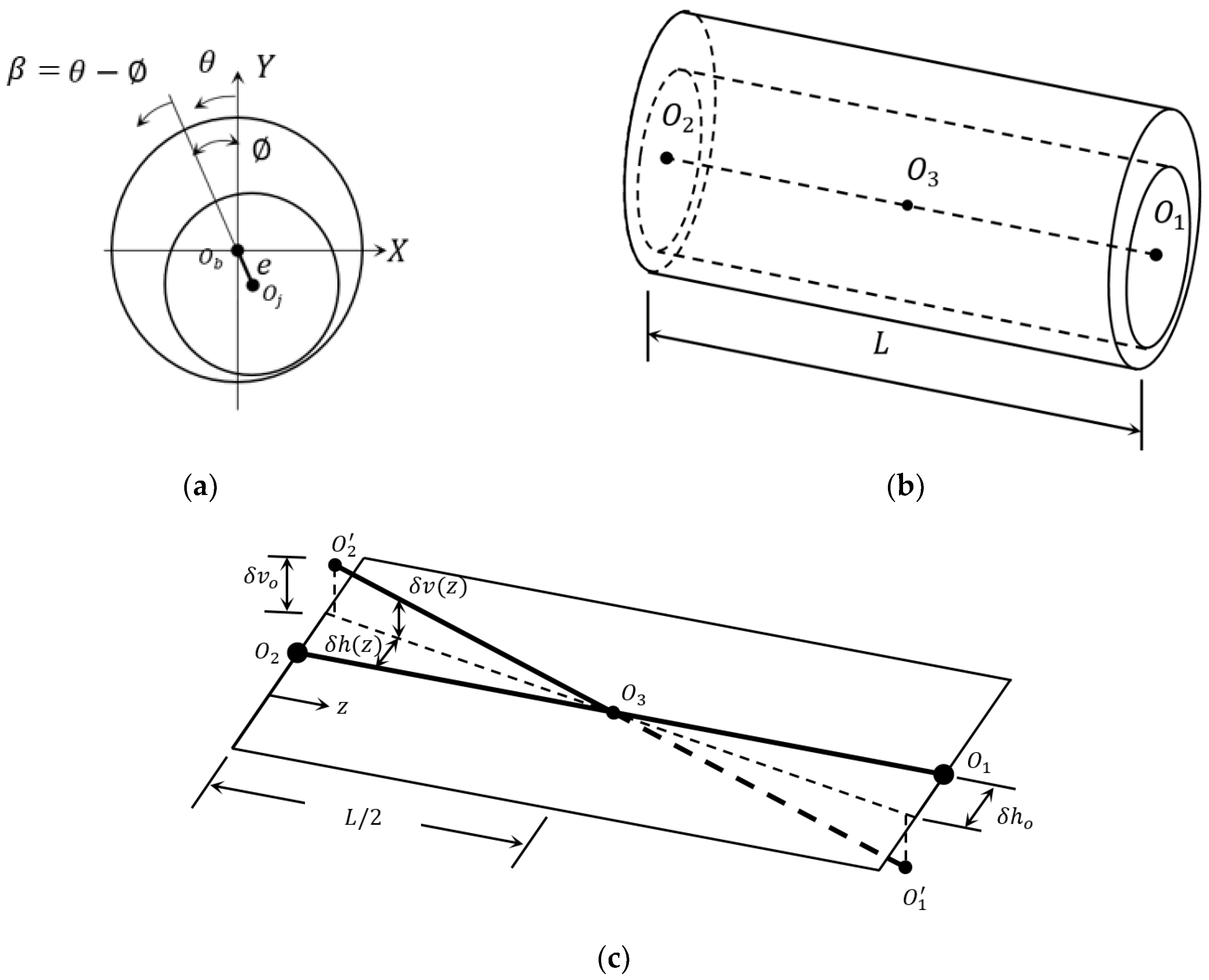
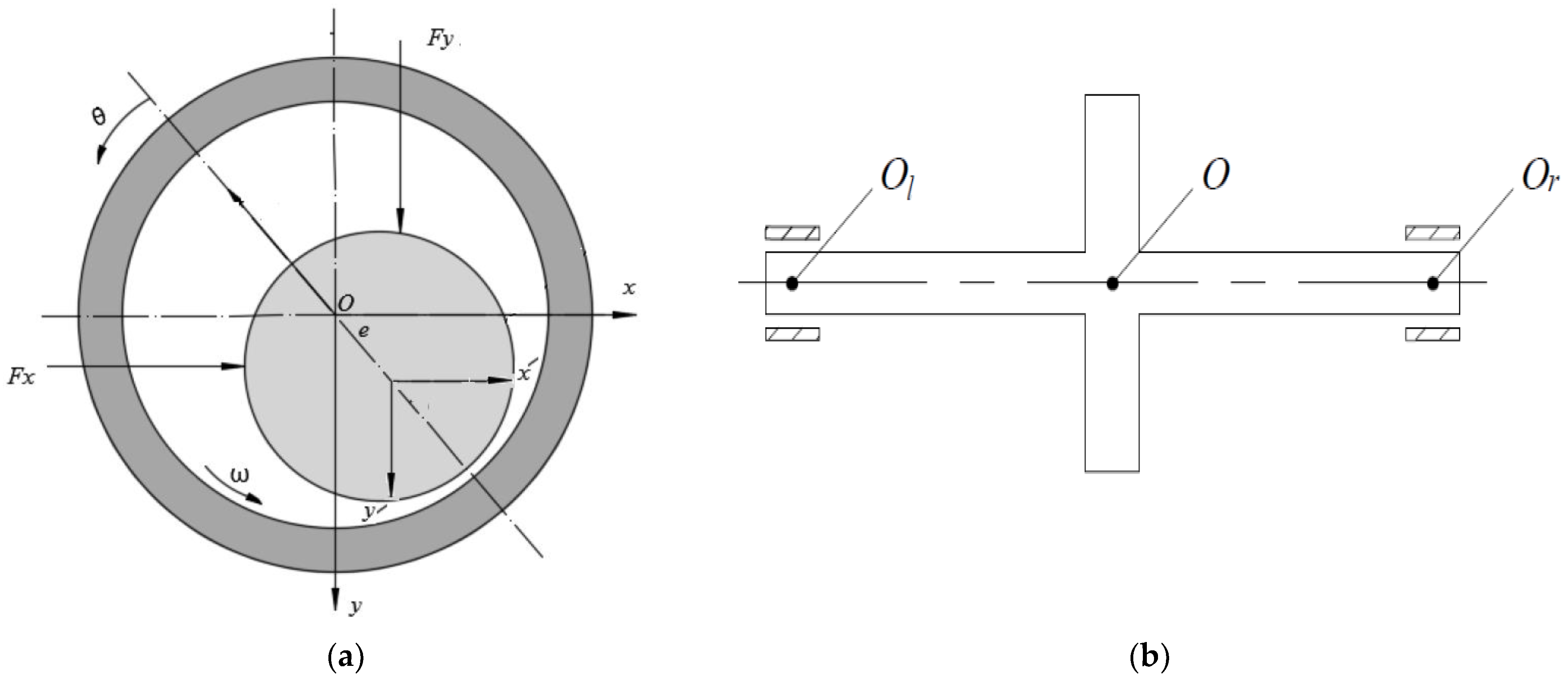
The general model used in this work is schematically shown in Figure 1. Figure 1a shows a side view of a perfectly aligned bearing, explaining the coordinates used in the analysis. Figure 1b illustrates a 3D representation for a journal bearing in its aligned case. As the model considers the misalignment effect, Figure 1c shows a general 3D misalignment model where the shaft deviations in the horizontal and vertical deviation along the bearing width are illustrated. More detail about this misalignment model can be found in [11,12]. 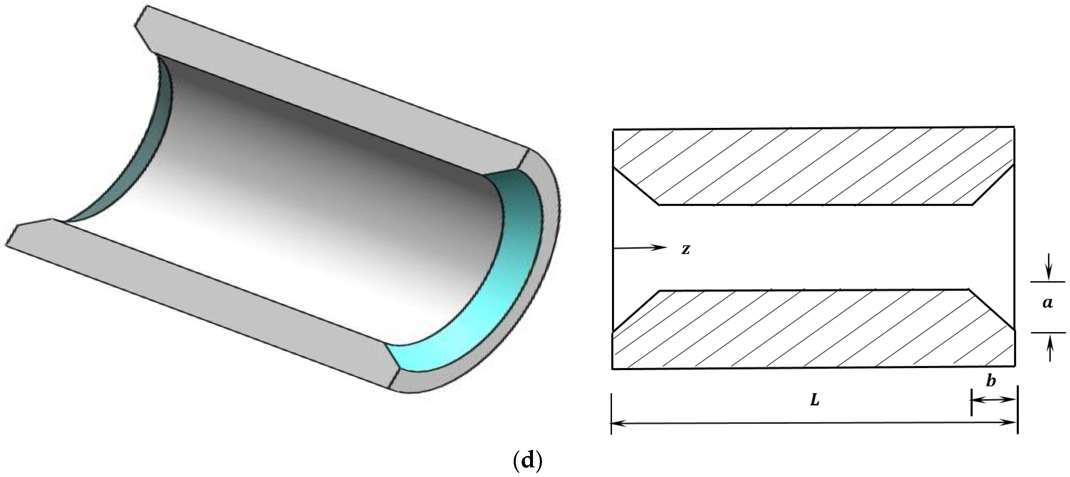The last figure (Figure 1d) shows the model used to incorporate the bearing profile variation in the solution of this hydrodynamic problem where the bearing edges are chamfered to reduce misalignment effects.

The governing equations related to the hydrodynamic solution of the journal-bearing problem are the Reynolds and the film thickness equations, which are given by [8,22]:

$$\frac{\partial }{\partial x}\left(\frac{\rho h^3}{12\eta }\frac{\partial p}{\partial x}\right)+\frac{\partial }{\partial z}\left(\frac{\rho h^3}{12\eta }\frac{\partial p}{\partial z}\right)=U_m \frac{\partial \rho h}{\partial x}+\frac{\partial \rho h}{\partial t}$$

(1)

$$h=c(1+{\epsilon }_r \cos \left(\theta -\varnothing \right))$$

(2)

where,

$\rho$, $\eta$: lubricant density and viscosity (Newtonian oil behavior)

$U_m$: mean velocity ($U_m=\frac{U_j+U_b}{2})$

p: pressure

h: film thickness

t: time

c: clearance

$\varnothing$: attitude angle

${\epsilon }_r$: eccentricity ratio (${\epsilon }_r=e/c$, e: eccentricity distance)

The density is constant in the case of incompressible flow, and the squeeze term is $\frac{\partial h}{\partial t}=0$ when the system operates under steady-state conditions, $U_{b=0}$ for stationary bearing and the journal, and surface velocity is $U_j=R\omega .$

The solution of Equation (1) is based on using the Reynolds boundary condition method [23]:

$$\begin{gathered} P=0\mathrm{at}\theta =0 \\ P=\frac{\partial P}{\partial \theta }=0\mathrm{at}\theta ={\theta }_{cav} \end{gathered}$$

The cavitation zone is limited by ${\theta }_{cav}$ and is identified by using an iteration method [23,24].

The governing equations will be written in dimensionless forms using the following dimensionless variables:

$$x=R\theta ,Z=\frac{z}{L},H=\frac{h}{c}$$

$$P=\frac{p-p_o}{6\eta \omega }(\frac{c^2}{R^2})$$

where

P: dimensionless pressure

H: dimensionless film thickness

L: bearing width

$p_o$: the atmospheric pressure

Therefore, Equations (1) and (2) becomes:

$$\frac{\partial }{\partial \theta }\left(H^3\frac{\partial P}{\partial \theta }\right)+\alpha \frac{\partial }{\partial Z}\left(H^3\frac{\partial P}{\partial Z}\right)-\frac{\partial H}{\partial \theta }=0$$

(3)

$$H=1+{\epsilon }_r \cos \left(\theta -\varnothing \right)$$

(4)

where

$$\alpha =\frac{R^2}{L^2}=\frac{1}{4{\left(L/D\right)}^2}$$

Integrating the resulting pressure field results in a dimensionless load [22]:

$$\overline{W}=\sqrt{{\overline{W_r}}^2+{\overline{W_t}}^2}$$

(5)

where

$$\overline{W_r}={{\displaystyle \int }}_0^1{{\displaystyle \int }}_0^{{\theta }_{cav}}P \cos \theta d\theta dz$$

(6)

$$\overline{W_t}={{\displaystyle \int }}_0^1{{\displaystyle \int }}_0^{{\theta }_{cav}}P \sin \theta d\theta dz$$

(7)

$$\overline{W}=\frac{w}{6\eta \omega RL}(\frac{c}{R}{)}^2$$

The attitude angle is given by [25].

$$\varnothing ={\tan }^{-1}(\frac{W_t}{W_r})$$

(8)

The general 3D misalignment model shown previously in Figure 1c, which is adapted from the work of the first author [8], is incorporated in the solution scheme using the following equations:

$$\begin{gathered} \Delta v\left(z\right)=\Delta v_o \left(1-2Z\right) for Z\le 1/2 \\ \Delta v\left(z\right)=\Delta v_o \left(2Z-1\right) for Z>1/2 \\ \Delta h\left(z\right)=\Delta h_o \left(1-2Z\right) for Z\le 1/2 \\ \Delta h\left(z\right)=\Delta h_o \left(2Z-1\right) for Z>1/2 \end{gathered}$$

(9)

where, $\Delta =\delta /c$, and $Z=z/L$ (dimensionless variables).

Using this 3D representation gives a more realistic modeling of the journal deviations in the vertical ($\Delta v\left(z\right))$ and horizontal directions $\left(\Delta h\left(z\right)\right)$ along the bearing width.

In the case of misalignment, the eccentricity, as well as the attitude angle, are no longer constant along the bearing width. They should be identified at each Z position along the bearing width, as given by [8]:

$$\varnothing \left(z\right)={\tan }^{-1}\frac{e\sin \varnothing +\delta h\left(z\right)}{e\cos \varnothing -\delta v\left(z\right)}\mathrm{for}z\le L/2$$

(10)

$$e\left(z\right)=\sqrt{{\left(e\cos \varnothing -\delta v\left(z\right)\right)}^2+{\left(e\sin \varnothing +\delta h\left(z\right)\right)}^2}$$

(11)

$$\varnothing \left(z\right)={\tan }^{-1}\frac{e\sin \varnothing -\delta h\left(z\right)}{e\cos \varnothing +\delta v\left(z\right)}\mathrm{for}z>L/2$$

(12)

$$e\left(z\right)=\sqrt{{\left(e\cos \varnothing +\delta v\left(z\right)\right)}^2+{\left(e\sin \varnothing -\delta h\left(z\right)\right)}^2}$$

(13)

where $\varnothing$ and $e$: the attitude angle and the eccentricity at $z=L/2$. These equations are used to calculate the new gap (due to misalignment) between the shaft and the bearing based on Equation (4).

The bearing with a variable profile was illustrated previously in Figure 1c. More detail about this profile variation can be found in [19]. The resulting gap in the circumferential direction related to this variation as a function of the z position along the bearing length is given by [19]:

$$\begin{gathered} G\left(z\right)=A (1-Z\frac{1}{B})\mathrm{for}Z\le B \\ G\left(z\right)=A (1+\frac{1}{B}\left(Z-1\right))\mathrm{for}Z\ge 1-B \\ G\left(z\right)=0\mathrm{for}B<Z<1-B \end{gathered}$$

(14)

where $A$ and $B$ (dimensionless) are: $A$ = $a/\mathrm{C}$ and $B=b/L$ (see Figure 1c).

These two dimensionless parameters are used to identify the effectiveness of varying the bearing profile. Dealing with the modification parameters in terms of the main bearing design parameters (c, L) provides the manufacturers with a more noticeable idea about the amount of required changes in the values of parameters related to the design of the bearing.

The coupling of Equations (4), (9) and (14) results in the total gap between the misaligned journal and the modified bearing. This gap is then used in the solution required to determine the static and dynamic characteristics of the bearing system.

The friction coefficient ($f$) can be determined using the following equation [26]:

$$f=\frac{\mathcal{F}}{W}$$

(15)

where $W$ is the supported load, $\mathcal{F}=\frac{\wp }{u}$ is the friction force, $u=R\omega$, $\wp$ is the power loss given by $\wp =\omega \sum {\displaystyle [}\eta R^3\omega {{\displaystyle \int }}_0^{\theta }l\frac{d\theta }{h}+\frac{1}{2}{\epsilon }_r(F_X\sin \varnothing -F_Y\cos \varnothing ){\displaystyle ]}$, and $F_X$ and $F_Y$ are the bearing forces in the horizontal and vertical directions, respectively. These forces can be easily calculated by integrating the pressure field.

3. Dynamic Characteristics

Following the linear stability analyses, the nonlinear hydrodynamic forces must be linearized around the journal steady state position to determine the stiffness and damping coefficients.

The equations of these eight coefficients are derived based on the time depending Reynolds equation, which is given by:

$$\frac{\partial }{\partial x}\left(\frac{h^3}{12\eta }\frac{\partial p}{\partial x}\right)+\frac{\partial }{\partial z}\left(\frac{h^3}{12\eta }\frac{\partial p}{\partial z}\right)=\frac{U_j}{2} \frac{\partial h}{\partial x}+\frac{\partial h}{\partial t}$$

(16)

The corresponding film equation is [27]:

$$h=h_0+\Delta x\cos \theta +\Delta y\sin \theta$$

(17)

Therefore, the $\frac{\partial h}{\partial t}$ term in Equation (16) can be written as

$$\frac{\partial h}{\partial t}=\Delta \dot{x}\cos \theta +\Delta \dot{y}\sin \theta$$

(18)

Substituting Equation (18) into Equation (16) and using dimensionless variables to get:

$$\frac{\partial }{\partial x}\left(\frac{h^3}{12\eta }\frac{\partial p}{\partial x}\right)+\frac{\partial }{\partial z}\left(\frac{h^3}{12\eta }\frac{\partial p}{\partial z}\right)=\frac{U}{2} \frac{\partial h}{\partial x}+\Delta \dot{x}\cos \theta +\Delta \dot{y}\sin \theta$$

(19)

Equation (19) can be written in a dimensionless form as:

$$\frac{\partial }{\partial \theta }\left(H^3\frac{\partial P}{\partial \theta }\right)+\alpha \frac{\partial }{\partial Z}\left(H^3\frac{\partial P}{\partial Z}\right)=\frac{\partial H}{\partial \theta }+2(\Delta \dot{Y}\sin \theta +\Delta \dot{X }\cos \theta )$$

(20)

where: $\dot{X}=\frac{R\dot{x}}{Uc}$, $\dot{Y}=\frac{R\dot{y}}{Uc}$.

The work of Lund and Thomson [26] is followed in this analysis where the x-axis is downward, but the results are reversed for the purpose of consistency with the system of coordinates adopted in this analysis.

The hydrodynamic forces are functions of $x$, $y$, $\dot{x}$, and $\dot{y}$ [25,26], which are:

$$\begin{gathered} F_x=F_x(x, y, \dot{x}, \dot{y}\left) \\ {F}_y=F_y(x, y, \dot{x}, \dot{y}\right) \end{gathered}$$

(21)

$$F_x={{\displaystyle \int }}_0^1{{\displaystyle \int }}_0^{{\theta }_{cav}}P\cos \theta d\theta dZ F_y={{\displaystyle \int }}_0^1{{\displaystyle \int }}_0^{{\theta }_{cav}}P\sin \theta d\theta dZ$$

(22)

where the total force is

$$F=\sqrt{F_x{}^2+F_y{}^2}.$$

The dynamic coefficients can be written in the following form [27]:

$$\left[k\right]=\left[\begin{array}{cc}{k}_{xx}& k_{xy}\\ k_{yx}& k_{yy}\end{array}\right]=\left[\begin{array}{cc}\frac{\partial F_x}{\partial X}& \frac{\partial F_x}{\partial Y}\\ \frac{\partial F_y}{\partial x}& \frac{\partial F_y}{\partial Y}\end{array}\right]$$

(23)

$$\left[c\right]=\left[\begin{array}{cc}{c}_{xx}& c_{xy}\\ c_{yx}& c_{yy}\end{array}\right]=\left[\begin{array}{cc}\frac{\partial F_x}{\partial \dot{X}}& \frac{\partial F_x}{\partial \dot{Y}}\\ \frac{\partial F_y}{\partial \dot{X}}& \frac{\partial F_y}{\partial \dot{Y}}\end{array}\right]$$

(24)

The eight dynamic coefficients are written based on the form used by [26]:

$$K_{xx}=\frac{c k_{xx}}{F},K_{xy}=\frac{c k_{xy}}{F},K_{yx}=\frac{c k_{yx}}{F},K_{yy}=\frac{c k_{yy}}{F}$$

(25)

$$C_{xx}=\frac{c\omega c_{xx}}{F},C_{xy}=\frac{c\omega c_{xy}}{F}, C_{yx}=\frac{c \omega c_{yx}}{F},C_{yy}=\frac{c \omega c_{yy}}{F}$$

(26)

Therefore, using Equations (23) and (24) to differentiate Equation (3) yields:

$$\begin{gathered} K_{xx}={{\displaystyle \int }}_0^1{{\displaystyle \int }}_0^{2\pi }{P}_x \cos \theta d\theta dz \\ {K}_{xy}={{\displaystyle \int }}_0^1{{\displaystyle \int }}_0^{2\pi }{P}_y \cos \theta d\theta dz \\ {K}_{yy}={{\displaystyle \int }}_0^1{{\displaystyle \int }}_0^{2\pi }{P}_y \sin \theta d\theta dz \\ {K}_{yx}={{\displaystyle \int }}_0^1{{\displaystyle \int }}_0^{2\pi }{P}_x \sin \theta d\theta dz \end{gathered}$$

(27)

Similarly, the damping coefficients are:

$$\begin{gathered} C_{xx}={{\displaystyle \int }}_0^1{{\displaystyle \int }}_0^{2\pi }{P}_{\dot{x}} \cos \theta d\theta dz \\ {C}_{xy}={{\displaystyle \int }}_0^1{{\displaystyle \int }}_0^{2\pi }{P}_{\dot{y}} \cos \theta d\theta dz \\ {C}_{yx}={{\displaystyle \int }}_0^1{{\displaystyle \int }}_0^{2\pi }{P}_{\dot{x}} \sin \theta d\theta dz \\ {C}_{yy}={{\displaystyle \int }}_0^1{{\displaystyle \int }}_0^{2\pi }{P}_{\dot{y}} \sin \theta d\theta dz \end{gathered}$$

(28)

where

$$P_x=\frac{\partial P}{\partial X},P_y=\frac{\partial P}{\partial Y},P_{\dot{x}}=\frac{\partial P}{\partial \dot{X}},P_{\dot{y}}=\frac{\partial P}{\partial \dot{Y}}$$

The other derivatives required to the determination of the dynamic coefficients are evaluated as follows:

$$\frac{\partial H}{\partial t}=\Delta \dot{X}\cos \theta +\Delta \dot{Y}\sin \theta$$

(29)

$$\frac{\partial H}{\partial X}=\cos \theta$$

(30)

$$\frac{\partial H}{\partial Y}=\sin \theta$$

(31)

$$\frac{\partial H}{\partial \theta }=-\Delta X \sin \theta +\Delta Y\cos \theta$$

(32)

The differentiation with respect to $X$ and Y gives:

$$\frac{\partial }{\partial \theta }\left(H^3\frac{\partial P_x}{\partial \theta }\right)+\alpha \frac{\partial }{\partial Z}\left(H^3\frac{\partial P_x}{\partial Z}\right)=-\frac{\partial }{\partial \theta }\left(3H^2\cos \theta \frac{\partial P}{\partial \theta }\right)-\alpha \frac{\partial }{\partial Z}\left(3H^2\cos \theta \frac{\partial P}{\partial Z}\right)-\sin \theta$$

(33)

$$\frac{\partial }{\partial \theta }\left(H^3\frac{\partial P_y}{\partial \theta }\right)+\alpha \frac{\partial }{\partial Z}\left(H^3\frac{\partial P_y}{\partial Z}\right)=-\frac{\partial }{\partial \theta }\left(3H^2\sin \theta \frac{\partial P}{\partial \theta }\right)-\alpha \frac{\partial }{\partial Z}\left(3H^2\sin \theta \frac{\partial P}{\partial Z}\right)-\cos \theta$$

(34)

Similarly, the differentiation with respect to $\dot{X}$ and $\dot{Y}$ yields:

$$\frac{\partial }{\partial \theta }\left(H^3\frac{\partial P_{\dot{x}}}{\partial \theta }\right)+\alpha \frac{\partial }{\partial Z}\left(H^3\frac{\partial P_{\dot{x}}}{\partial Z}\right)=\cos \theta$$

(35)

$$\frac{\partial }{\partial \theta }\left(H^3\frac{\partial P_{\dot{y}}}{\partial \theta }\right)+\alpha \frac{\partial }{\partial Z}\left(H^3\frac{\partial P_{\dot{y}}}{\partial Z}\right)=\sin \theta$$

(36)

Equations (33)–(36) require a numerical solution in order to determine the pressure derivatives related to the calculation of $K_{xx}$, $K_{xy}$, $K_{yx}$, $K_{yy}$, $C_{xx}$, $C_{xy}$ and $C_{yx},$ which will be explained later.

4. Stability of the System

After determining the dynamic coefficients, the critical speed and the time response of the bearing system can be identified. The system is stable if the operating rotational speed is less than the critical speed value. The dangerous journal whirling, which is related to the stability of the system, takes place around the steady state (equilibrium) position [28]. The equations of motion for the rigid rotor shown in Figure 2, which is supported by journal bearings, are given by [28]

$$m{\ddot{x}}^{\prime }=-F_x+f_{ex}-f\sin \Omega t$$

(37)

$$m{\ddot{y}}^{\prime }=-F_y+f_{ey}-f\cos \Omega t+W$$

(38)

where [29] $F_x\mathrm{and}{F}_y$ are the bearing forces, $f$ is the unbalance force, $f_{ex}$ and $f_{ey}$ are the external loads. $x^{\prime }$ and $y^{\prime }$ are the axes of whirling of the shaft center around its equilibrium position.

Equations (37) and (38) are written in dimensionless form as:

$$\overline{M}{\ddot{X}}^{\prime }=-{\overline{F}}_x+{\overline{F}}_{ex}-\overline{Ru} \sin T$$

(39)

$$\overline{M}{\ddot{Y}}^{\prime }=-{\overline{F}}_y+{\overline{F}}_{ey}-\overline{Ru}\cos T+1$$

(40)

where

$$\overline{M}=\frac{mc{\Omega }^2}{W},{\overline{F}}_x=\frac{F_x}{W} \mathrm{and}\overline{\mathrm{Ru}}=m_u\mathrm{r}\frac{{\Omega }^2}{W}$$

The solution of the equations of motion is essential in determining the dynamic response of the system [30]. Neglecting the unbalanced and external forces, the critical speed can be determined using the solution of the following linear equations:

$$\overline{M}{\ddot{X}}^{\prime }+{\overline{F}}_x=0$$

(41)

$$\overline{M}{\ddot{Y}}^{\prime }+{\overline{F}}_y=0$$

(42)

The bearing forces can be written for small displacement around the steady state position as [26]:

$$\overline{F}x=K_{xx}{X}^{\prime }+K_{xy}{Y}^{\prime }+C_{xx}{\dot{X}}^{\prime }+C_{xy}{\dot{Y}}^{\prime }$$

(43)

$$\overline{F}y=K_{yx}{X}^{\prime }+K_{yy}{Y}^{\prime }+C_{yx}{\dot{X}}^{\prime }+C_{yy}{\dot{Y}}^{\prime }$$

(44)

Substitution of these two Equations (43) and (44) in Equations (41) and (42) yields:

$$\overline{M}{\ddot{X}}^{\prime }+K_{xx} X^{\prime }+K_{xy} Y^{\prime }+C_{xx}{\dot{X}}^{\prime }+C_{xy}{\dot{Y}}^{\prime }=0$$

(45)

$$\overline{M}{\ddot{Y}}^{\prime }+K_{yx} X^{\prime }+K_{yy} Y^{\prime }+C_{yx}{\dot{X}}^{\prime }+C_{yy}{\dot{Y}}^{\prime }=0$$

(46)

The solution for these two equations are [31]:

$$X^{\prime }=\mathrm{A}{e}^{i\lambda t},Y^{\prime }=\mathrm{B}{e}^{i\lambda t}$$

(47)

Substitution of these solutions in Equations (45) and (46) gives:

$$\left(keq-K_{xx}\right)\left(keq-K_{yy}\right)-{\lambda }^2{C}_{xx}{C}_{yy}-K_{xy} K_{yx}+{\lambda }^2 C_{xy}{C}_{yx}=0$$

(48)

where

$$\lambda =\sqrt{\frac{\left(keq-K_{xx}\right)\left(Keq-K_{yy}\right)-K_{xy} K_{yx}}{C_{xx}{C}_{yy}-C_{xy}{C}_{yx}}}$$

(49)

$$Keq=\frac{K_{xx}{C}_{yy}+K_{yy}{C}_{xx}-K_{yx}{C}_{xy}-K_{xy}{C}_{yx}}{C_{xx}+C_{yy}}$$

(50)

The critical speed (${\Omega }_{crit}$) is:

$${\Omega }_{crit}=\frac{\sqrt{keq}}{\lambda }$$

(51)

5. Numerical Solution

The determination of the eight dynamic coefficients requires a numerical solution for the governing equations illustrated previously. Following this determination, the equations of motion can be solved numerically in order to determine the time responses of the system to the position perturbation in addition to the identification of the stability limits of the system. The solution of these equations is based on using a fourth-order Runge-Kutta method. The solution plane for the variable profile bearing hydrodynamic problem under misalignment conditions is a rectangle where the nodes are distributed in the circumferential and longitudinal directions. The successive over-relaxation method is used in order to obtain a relatively faster convergence for the Gauss–Sedial method.

Discretizing the related equations yields the following equations:

$$P_{\left(i,j\right)}=\frac{1}{\beta }\left[H_b{}^3 P_{\left(i+1,j\right)}+H_a{}^3 P_{\left(i-1,j\right)}+\alpha C_2{H}_c{}^3 P_{\left(i,j+1\right)}+\alpha C_2{H}_d{}^3 P_{\left(i,j-1\right)}-C_1{H}_{\left(i+1,j\right)}+C_1{H}_{\left(i-1,j\right)}\right]$$

(52)

where $\alpha =\frac{R^2}{L^2}$, $C_1=\frac{\Delta \theta }{2}$, $C_2=\frac{{(\Delta \theta )}^2}{{(\Delta Z)}^2}$, $\beta =H_b{}^3+H_a{}^3+\alpha C_2{H}_c{}^3+\alpha C_2{H}_d{}^3$, $\Delta Z$ and $\Delta \theta$ are the mesh steps.

The lubricant film in terms of $i, j$ position is:

$$H\left(i,j\right)=\left(1+{\epsilon }_r\left(Z\right)\cos ({\theta }_{\left(i,j\right)}-\varnothing \right))$$

(53)

More details about the solution method can be found in [8].

The convergence condition of the pressure values is given by $\frac{\sum \left|P_{\left(i,j\right)new}-P_{\left(i,j\right)old}\right|}{\sum P_{\left(i,j\right)old}}<{10}^{-7}$. Furthermore, after obtaining the pressure convergence, the resultant hydrodynamic load is calculated. This load is then compared with the actual supported load to achieve an accurate load condition of $\mp {10}^{-5}$. If this condition is not satisfied, the eccentricity ratio changes, and the pressure field is again determined based on the newly updated eccentricity ratio. This process is repeated until the load (as well as the pressure) convergence is achieved. This load corresponds to ${\epsilon }_r=0.6$ in the aligned case. A flow chart for the general solution procedure is shown in Figure 3. After obtaining the solution convergences, the stuffiness and damping coefficients are calculated, and then the time responses to the position perturbation are determined by solving the equations of motion based on the Runge–Kutta method.

The numerical solution of Equations (33)–(36) is required to calculate the dynamic coefficients. Using the finite difference method to discretize these equations yields the following general equation to determine the corresponding pressure derivative (${\overline{P}}_{\left(i.j\right)})$:

$${\overline{P}}_{\left(i.j\right)}=\frac{1}{\psi }\left[{\left(\Delta \theta \right)}^2 RHS-H_b{}^3 {\overline{P}}_{\left(i+1.j\right)}-H_a{}^3 {\overline{P}}_{\left(i-1.j\right)}-\alpha C_2{H}_c{}^3 {\overline{P}}_{\left(i.j+1\right)}-\alpha C_2{H}_d{}^3 {\overline{P}}_{\left(i.j-1\right)}+C_1{H}_{\left(i+1.j\right)}-C_1{H}_{\left(i-1.j\right)}\right]$$

(54)

where $\alpha =\frac{R^2}{L^2}$, $C_1=\frac{\Delta \theta }{2}$, $C_2=\frac{{(\Delta \theta )}^2}{{(\Delta Z)}^2}$ and $\psi =-H_b{}^3-H_a{}^3-\alpha C_2{H}_c{}^3-\alpha C_2{H}_d{}^3$.

The right side of Equations (33)–(36) can be calculated numerically using the following equations:

$$\begin{gathered} RHS\left(19\right)=\frac{\left(3\cos {\theta }_b{H}_b^2+3\cos {\theta }_a{H}_a^2\right)P_{\left(i.j\right)}}{{\left(\Delta \theta \right)}^2}-\frac{3\cos {\theta }_b{H}_b^2{P}_{\left(i+1.j\right)}}{{\left(\Delta \theta \right)}^2}-\frac{3\cos {\theta }_a{H}_a^2{P}_{\left(i-1.j\right)}}{{\left(\Delta \theta \right)}^2}+ \\ \alpha \frac{\left(3\cos {\theta }_c{H}_c^2+3\cos {\theta }_d{H}_d^2\right)P_{\left(i.j\right)}}{{\left(\Delta Z\right)}^2}-\alpha \frac{3\cos {\theta }_c{H}_c^2{P}_{\left(i.j+1\right)}}{{\left(\Delta Z\right)}^2}-\alpha \frac{3\cos {\theta }_d{H}_d^2{P}_{\left(i.j-1\right)}}{{\left(\Delta Z\right)}^2}-\sin \theta \end{gathered}$$

(55)

$$\begin{gathered} RHS\left(20\right)=\frac{\left(3\sin {\theta }_b{H}_b^2+3\sin {\theta }_a{H}_a^2\right)P_{\left(i.j\right)}}{{\left(\Delta \theta \right)}^2}-\frac{3\sin {\theta }_b{H}_b^2{P}_{\left(i+1.j\right)}}{{\left(\Delta \theta \right)}^2}-\frac{3\sin {\theta }_a{H}_a^2{P}_{\left(i-1.j\right)}}{{\left(\Delta \theta \right)}^2}+ \\ \alpha \frac{\left(3\sin {\theta }_c{H}_c^2+3\sin {\theta }_d{H}_d^2\right)P_{\left(i.j\right)}}{{\left(\Delta Z\right)}^2}-\alpha \frac{3\sin {\theta }_c{H}_c^2{P}_{\left(i.j+1\right)}}{{\left(\Delta Z\right)}^2}-\alpha \frac{3\sin {\theta }_d{H}_d^2{P}_{\left(i.j-1\right)}}{{\left(\Delta Z\right)}^2}-\cos \theta \end{gathered}$$

(56)

$$RHS\left(21\right)=\cos {\theta }_{\left(i.j\right)}$$

(57)

$$RHS\left(22\right)=\sin {\theta }_{\left(i.j\right)}$$

(58)

6. Results and Discussions

The numerical model used in this work is firstly examined in terms of the required numbers of nodes and time steps to ensure the independence of the analysis on the discretization density (16,471 nodes have been found to be sufficient enough for the solution). Furthermore, the calculated critical speed is compared with the well-known work of Lund and Thomson [26] for the purpose of verification.

Table 1. Verification of the current work (L/D = 1).

${\mathit{\epsilon }}_{\mathit{r}}$	Current Work	Lund and Thomson	% Diff.
0.15	2.0901	2.0966	0.31139
0.352	2.0909	2.1096	0.88648
0.559	2.1559	2.1714	0.71303
0.734	2.7871	2.8217	1.22693

shows this comparison for different values of the eccentricity ratio and $L/D=1$. The maximum difference is only 1.23% at a high eccentricity ratio. The agreement is also excellent at the lower values of the eccentricity ratio. The results presented in this work are obtained for a bearing with $L/D=1.25$ and a supported load corresponding to an ideal case where the eccentricity ratio is 0.6.

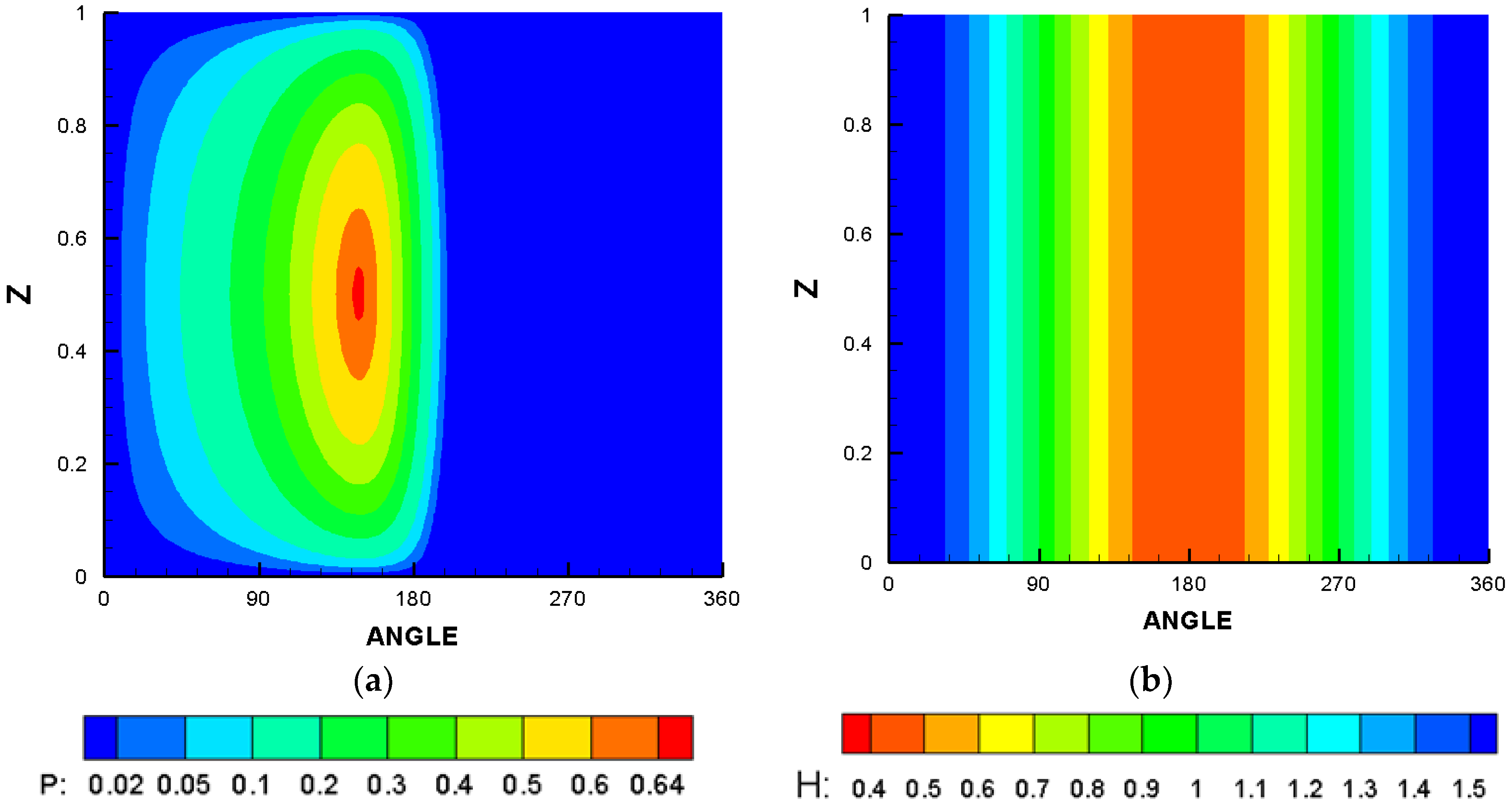
The results of the solution for the case of the perfectly aligned bearing are shown in Figure 4 for a finite length bearing where $L/D=1.25$ and the eccentricity ratio (${\epsilon }_r$) is 0.6. Figure 4a shows the dimensionless pressure distribution, and Figure 4b illustrates the dimensionless film thickness levels. The determination of the cavitation zone is important for the purpose of obtaining the correct solution for the hydrodynamic problem of the journal bearing as the pressure generation extends beyond the position of 180°, as shown in Figure 4a. It can be seen that the pressure distribution is symmetrical with the center of the bearing width ($Z \mathrm{direction}$), where its maximum value is at this position. In addition, the film thickness levels are also symmetrical with the position of minimum film thickness where the angle in the circumferential direction is 180°. Furthermore, the film thickness value at any position in the circumferential direction is constant (extruded shape) along the bearing width. However, this ideal situation rarely exists in the typical usages of this type of bearing as the bearing system is usually subjected to some degree of misalignment, which affects the shape and the values of the film and pressure distributions.

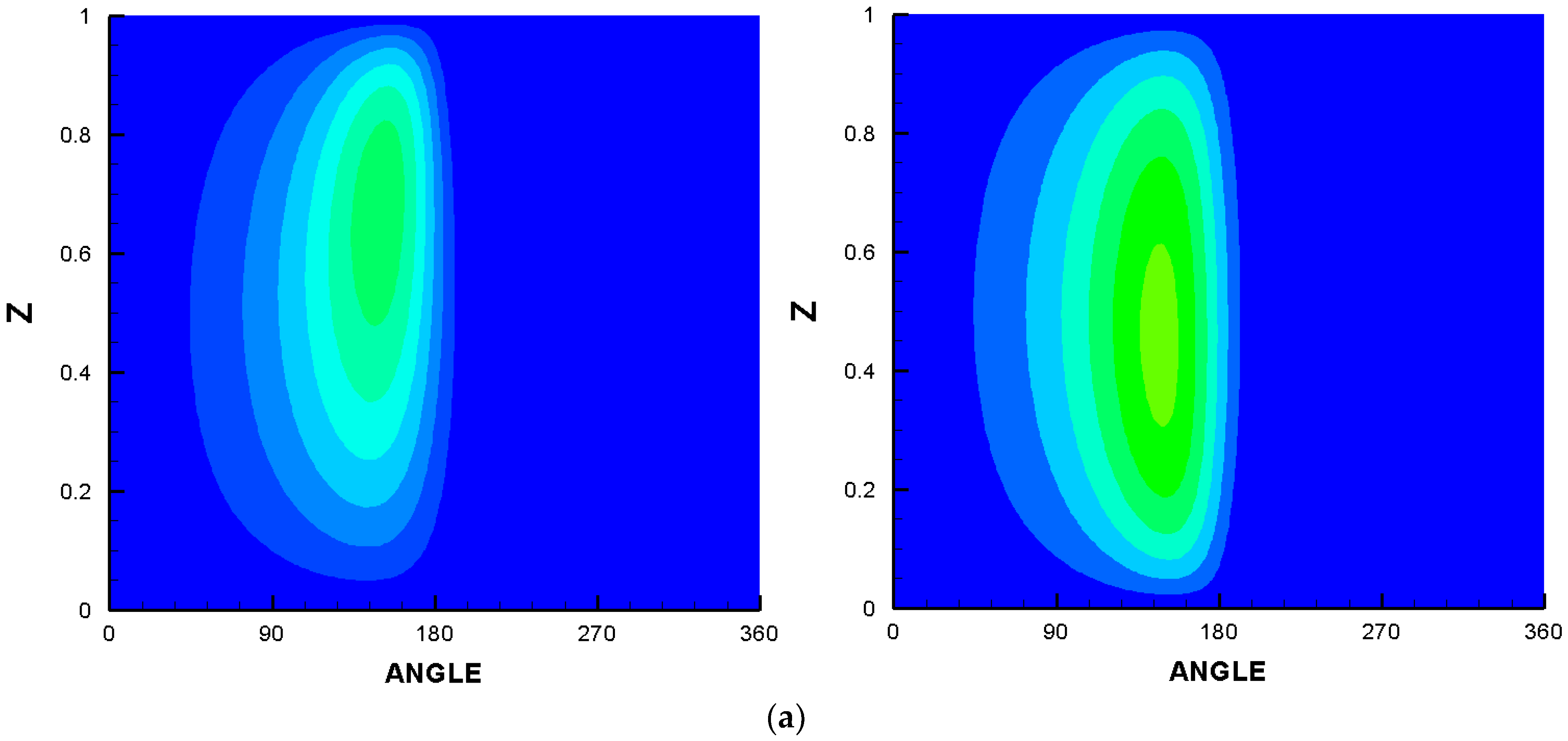
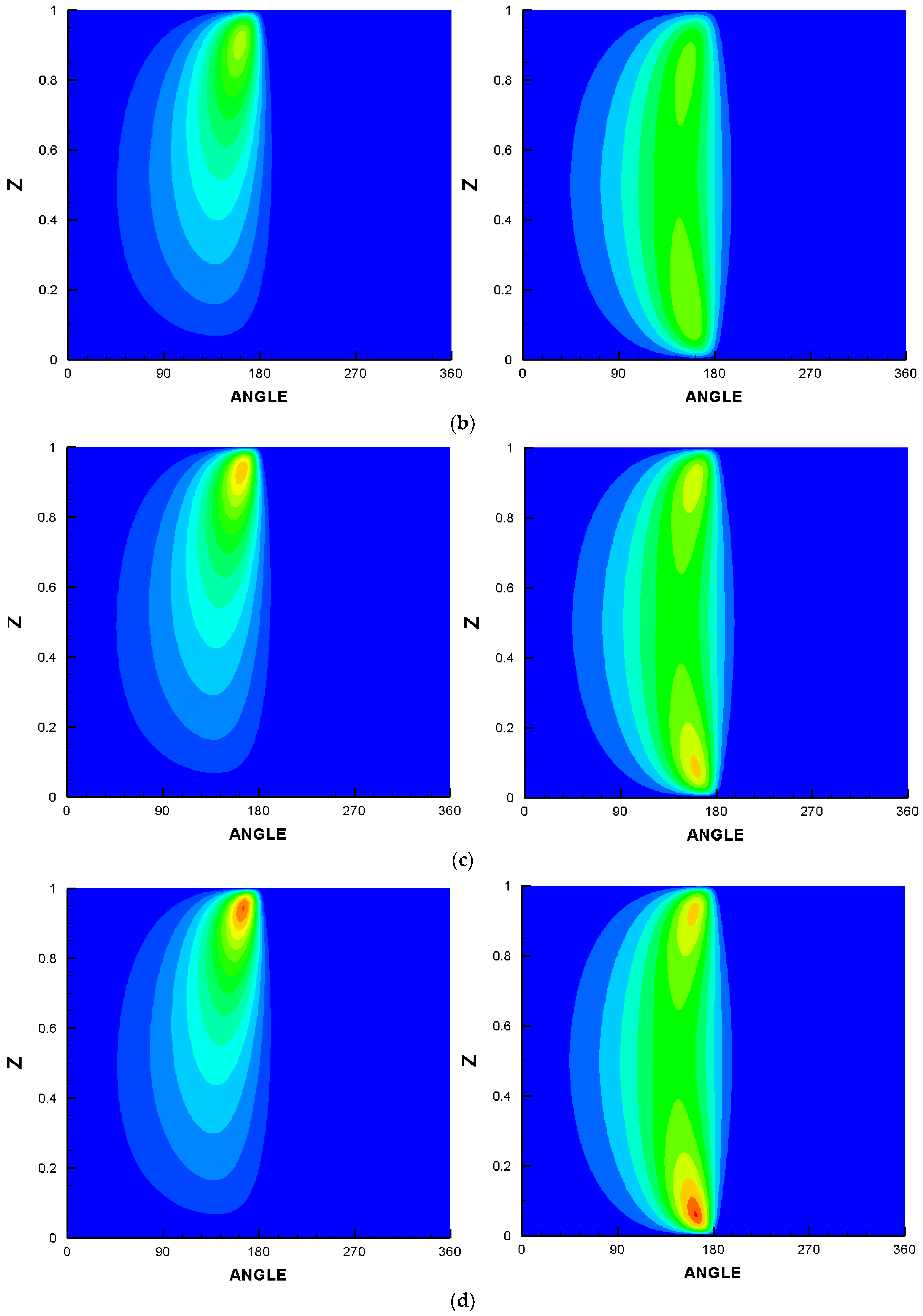
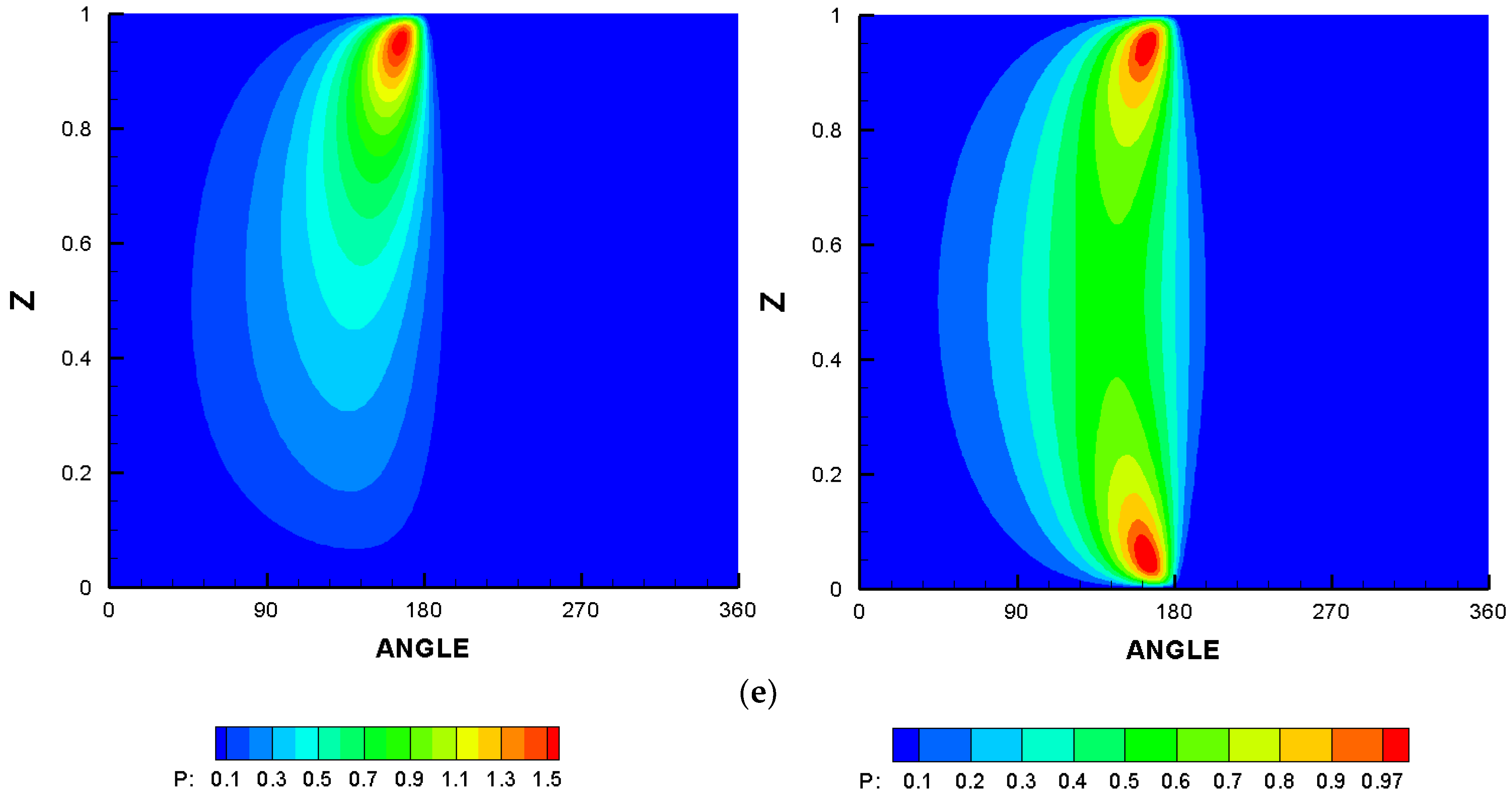
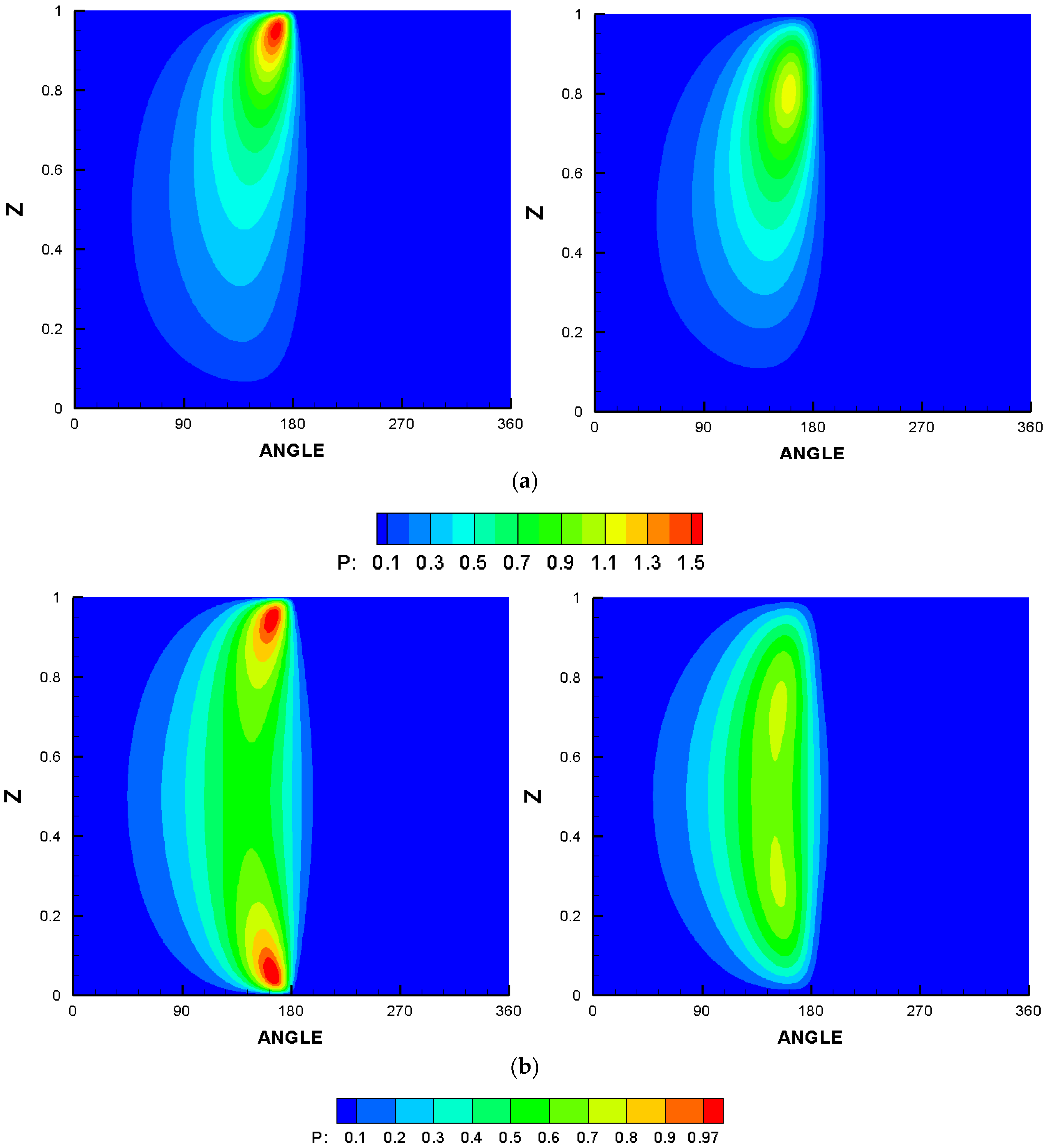
Figure 5 illustrates this concept, where two cases of misalignment are considered. The dimensionless pressure distributions on the left side correspond to the misalignment case in the vertical direction only, while the right side shows the pressure distributions for the general case of 3D misalignment where the shaft deviation takes place in the vertical and horizontal directions. The misalignment due to only horizontal deviation is not considered, as the vertical misalignment usually accompanies the journal bearing system as a result of shaft deformation under the supported load. It is worth mentioning that each side has a different legend, as using a single unified legend does not give a clear picture of the differences between the two cases. Five values for the misalignment parameters are examined in this figure for each case, which are $\Delta v=0.2,0.5,0.55,0.57\mathrm{and}0.59$ for the first case and $\Delta v=\Delta h=0.2,0.5,0.55,0.57\mathrm{and}0.59$ for the second 3D case. These values range from light to extreme levels of misalignment. In comparison with the pressure distribution of the perfectly aligned bearing shown previously in Figure 4, two distinguished features can be observed from the results shown in Figure 5. The first thing is that the maximum pressure increased significantly as the misalignment parameters increased and concentrated close to the bearing edge, where the misalignment effect is the maximum in reducing the gap between the shaft and the bearing wall. The second issue is that the pressure distribution is no longer symmetrical due to the misalignment. These two features are more clear at the extreme levels of misalignment, particularly in the last case, Figure 5e, where the misalignment parameter is 0.59. Furthermore, the vertical misalignment negatively affects the pressure distribution in terms of the maximum pressure values and the asymmetricity in the distribution of the pressure levels. However, the 3D misalignment, as will be shown later, has a larger drawback regarding the friction coefficient.

As explained previously, the perfect alignment of the bearing system is hard to achieve in industrial applications, where the presence of misalignment is actually unavoidable. Using a variable profile in the longitudinal bearing direction can be used to reduce the misalignment effect by reducing the pressure levels and increasing the minimum film thickness, which means, in other words, extending the life of the bearing. Figure 6 illustrates this effect where the bearings in the last extreme cases shown in the previous figure (Figure 5e) are modified. The pressure distributions of Figure 5e are repeated here for the purpose of comparison with the modified bearings. The modification parameters used in this figure are $A=B=0.25$ (more details about the effect of the modification parameters will be explained later in the following figures). Figure 6a shows the modification effect on the pressure distribution of the bearing system when the misalignment presents in the vertical direction. The maximum pressure value was reduced by 26.6% (from 1.58 to 1.16) due to this modification. The pressure spike is relatively shifted away from the bearing edge, which may help prevent the bearing wear at the bearing edge. Similar behavior can be seen in the case of 3D misalignment, as shown in Figure 6b, where $P_{max}$ is reduced by 29.2% (from 1.06 to 0.75) in addition to shifting the pressure spikes from the bearing edges.

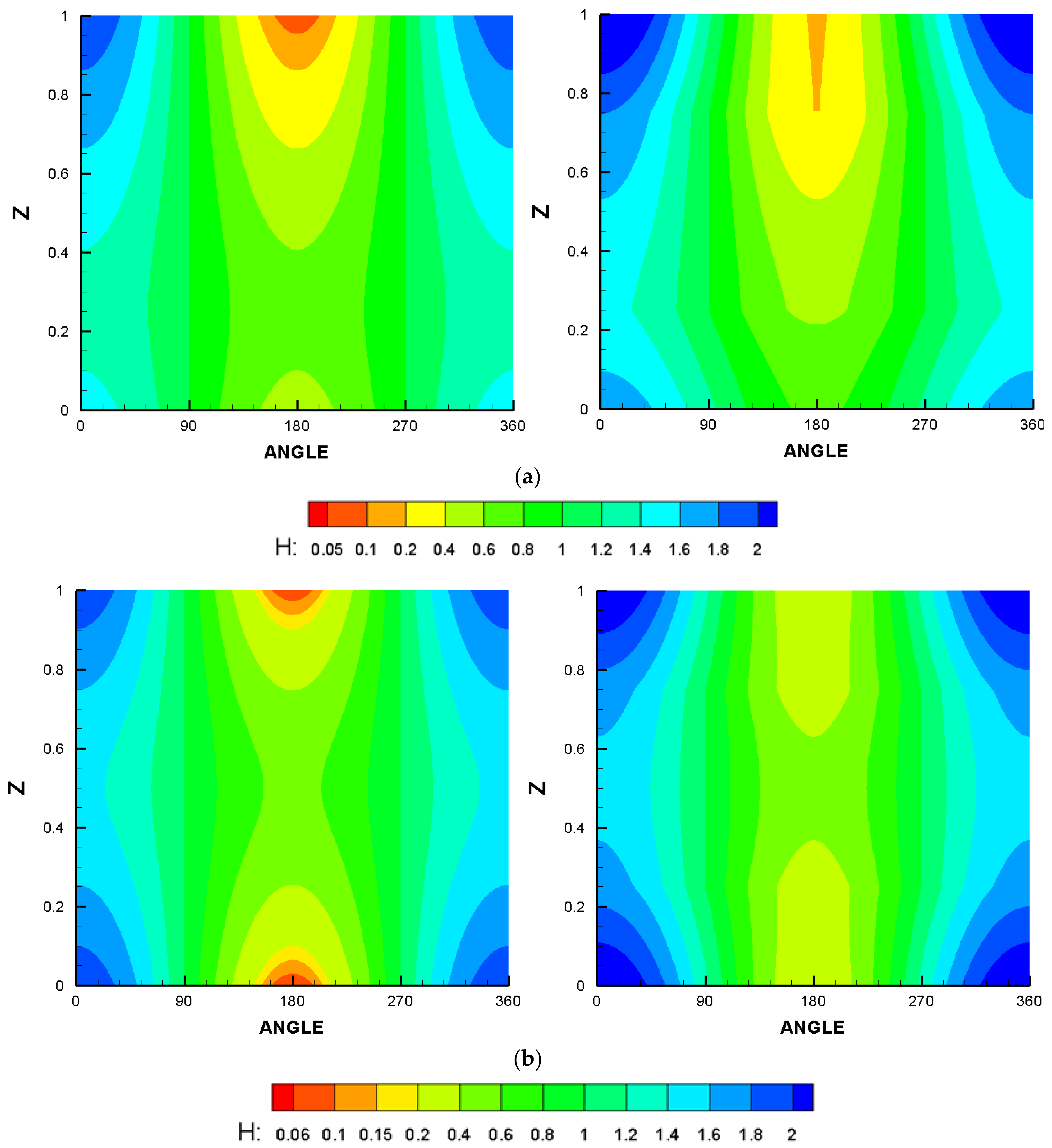
The corresponding effect of the modification on the level of the dimensionless film thickness for the severe misalignment case illustrated in Figure 5e (misalignment parameter is 0.59) is shown in Figure 7. The minimum film thickness decreases from 0.4 for the case of a perfectly aligned bearing (see Figure 4b) to 0.0495 for the case when the misalignment is in the vertical direction only, as shown in Figure 7a. The bearing profile modification helps in elevating $H_{min}$ to be 0.1887 as shown on the right side of this figure. The corresponding results of the minimum film thickness for the 3D misalignment case are shown in Figure 7b. This case of misalignment reduces the film thickness to 0.0572 in comparison with 0.4 for the ideal aligned case (see Figure 4b).

The bearing modification elevates the level of $H_{min}$ to 0.2443. In the two cases of the severe level of misalignment, introducing the bearing profile modification significantly improves the levels of film thickness. This is an expected outcome due to the resulting change in the geometry to compensate for the loss of the sufficient gap between the bearing walls and the surface of the shaft due to the misalignment.

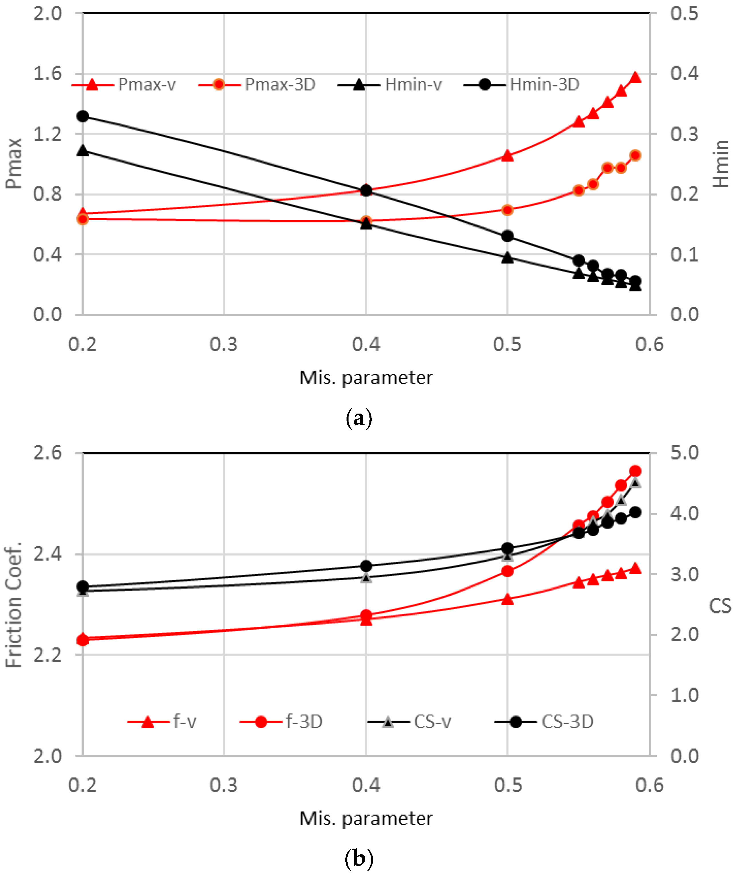
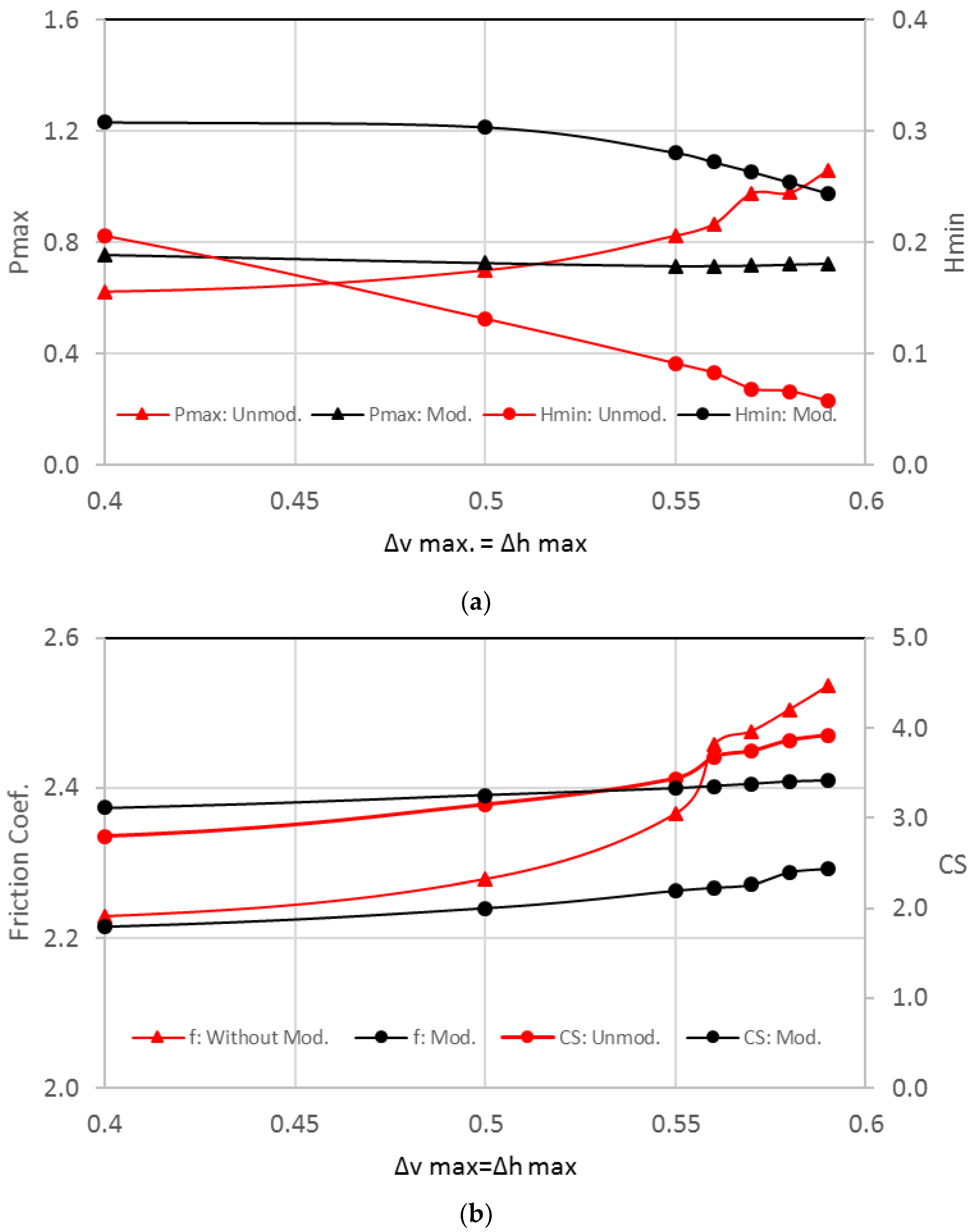
The comparison between the two cases of misalignment is extended to include their effects on the friction coefficient in addition to more detail about the misalignment consequences on $P_{max}$ and $H_{min}$ for a wide range of misalignment parameters. Figure 8 illustrates these comparisons where Figure 8a shows the variations in $P_{max}$ and $H_{min}$ and Figure 8b illustrates the comparisons in terms of the friction coefficient and critical speed. The misalignment parameters are a range of $\Delta v$ ($\Delta h=0$) for the vertical misalignment case and arrange as $\Delta v=\Delta h$ for the 3D misalignment case. The vertical and 3D misalignment increases $P_{max}$ and reduces $H_{min}$ for the whole range of the modification parameters, as shown in Figure 8a, with a more negative influence associated with the vertical misalignment case. On the other hand, the friction coefficient in both cases is not significantly affected by the presence of misalignment when the misalignment parameter is relatively low (≤0.4), but as this parameter increases, the friction coefficient starts to increase in both cases. It can be seen that the case of 3D misalignment causes significant increases in the coefficient of friction in comparison with the vertical misalignment case, particularly at the extreme levels of misalignment parameters. The friction coefficient for the perfectly aligned case is 2.2181, which increases to 2.3718 and 2.5643 for the vertical and 3D misalignment cases, respectively, when the misalignment parameter is 0.59. This represents an increase of 6.92% and 15.6% for the vertical and 3D misalignment cases, respectively. This increase in the friction coefficient of the 3D misalignment case in comparison with the vertical misalignment case can be attributed to the resulting geometry of the gap between the shaft surface and the bearing wall. As the shaft deviates in the vertical and horizontal direction in the 3D misalignment case, the shaft surface becomes closer to the bearing wall over a relatively wider area, leading to an increase in the coefficient of friction. This Figure also shows that the dimensionless critical speeds in both cases are increased with the increasing misalignment parameters. The significant changes in the friction coefficient and the critical speed occur when the $\Delta v \left(\mathrm{or} \Delta v=\Delta h\right)\ge 0.4$. Therefore, this range of misalignment will be investigated in the following Figures, where the bearing profile modification is introduced to reduce the misalignment consequences on the bearing characteristics.

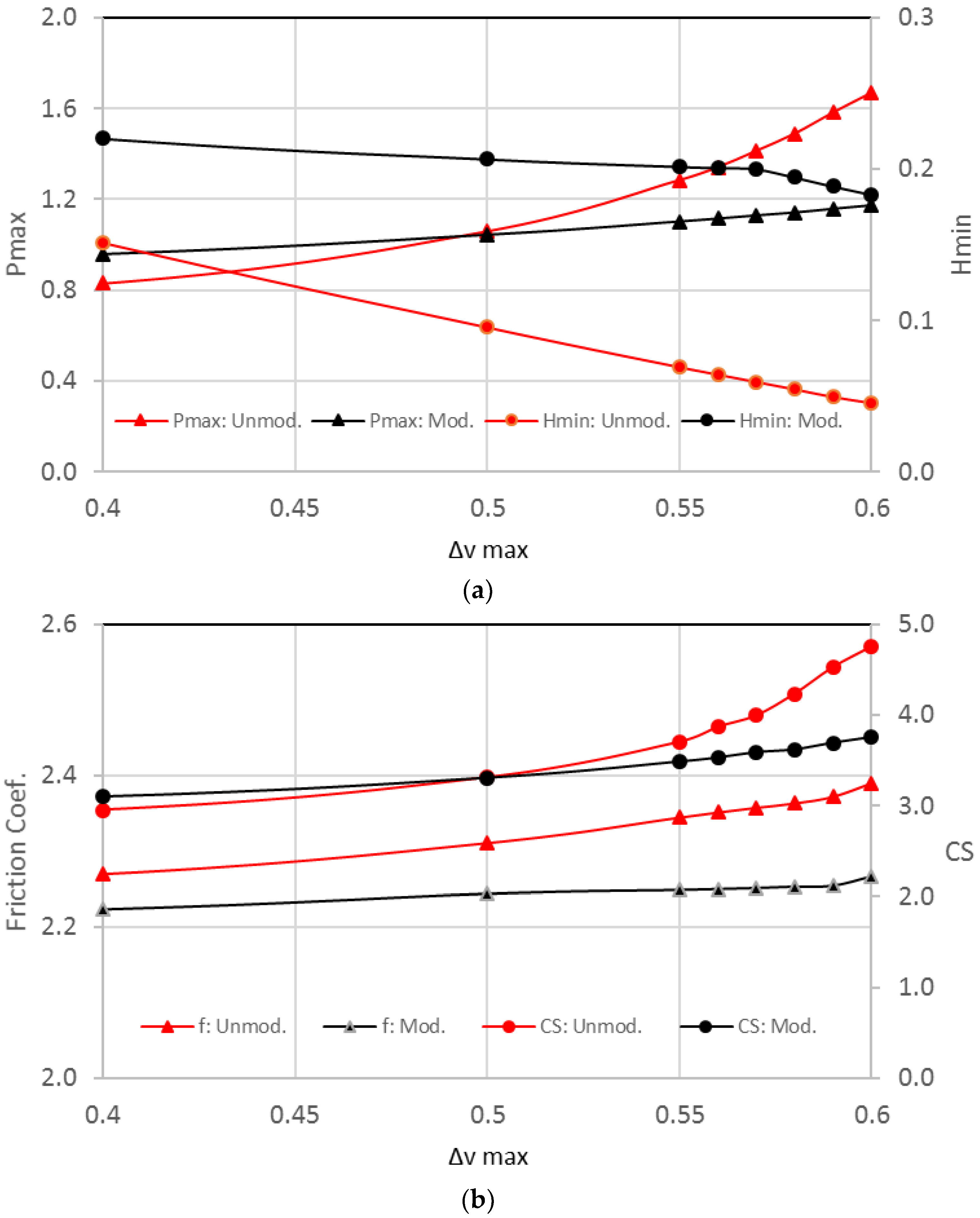
Figure 9 shows the effect of bearing profile modification on the bearing characteristics for the first case of vertical misalignment when the modification parameters are $A=B=0.25$. Figure 9a illustrates this effect on $P_{max}$ and $H_{min}$ where the modification reduces the maximum pressure and increases the minimum film thickness. The reduction in $P_{max}$ is 26.6% and the increase in $H_{min}$ is about three times the corresponding unmodified misaligned bearing when $\Delta v=0.59$ as explained previously. The corresponding effects of profile modification on the friction coefficient and the critical speed for the first case of vertical misalignment are shown in Figure 9b. It can be seen that the friction coefficient is reduced by 4.97% (from 2.3718 to 2.2539). The critical speed of the misaligned bearing, on the other hand, is also reduced as a result of the modification, but the positive thing is that the critical speed for the modified bearing (3.6906) is greater than that of the perfectly aligned bearing (2.6789).

The corresponding results of the effect of profile modification on the bearing characteristics of the second case of 3D misalignment are shown in Figure 10. In general, similar behaviors have been obtained for all bearing characteristics. The friction coefficient is reduced by 9.76% (from 2.5357 to 2.2881), representing a significant gain for the profile modification in addition to improvement in the minimum film thickness levels and the reduction in the maximum pressure values. Furthermore, despite the reduction in the critical speed due to the profile modification compared with the misaligned case, there is an improvement in the critical speed of the modified bearing (3.4121) compared with the aligned case where the critical speed is 2.6789.

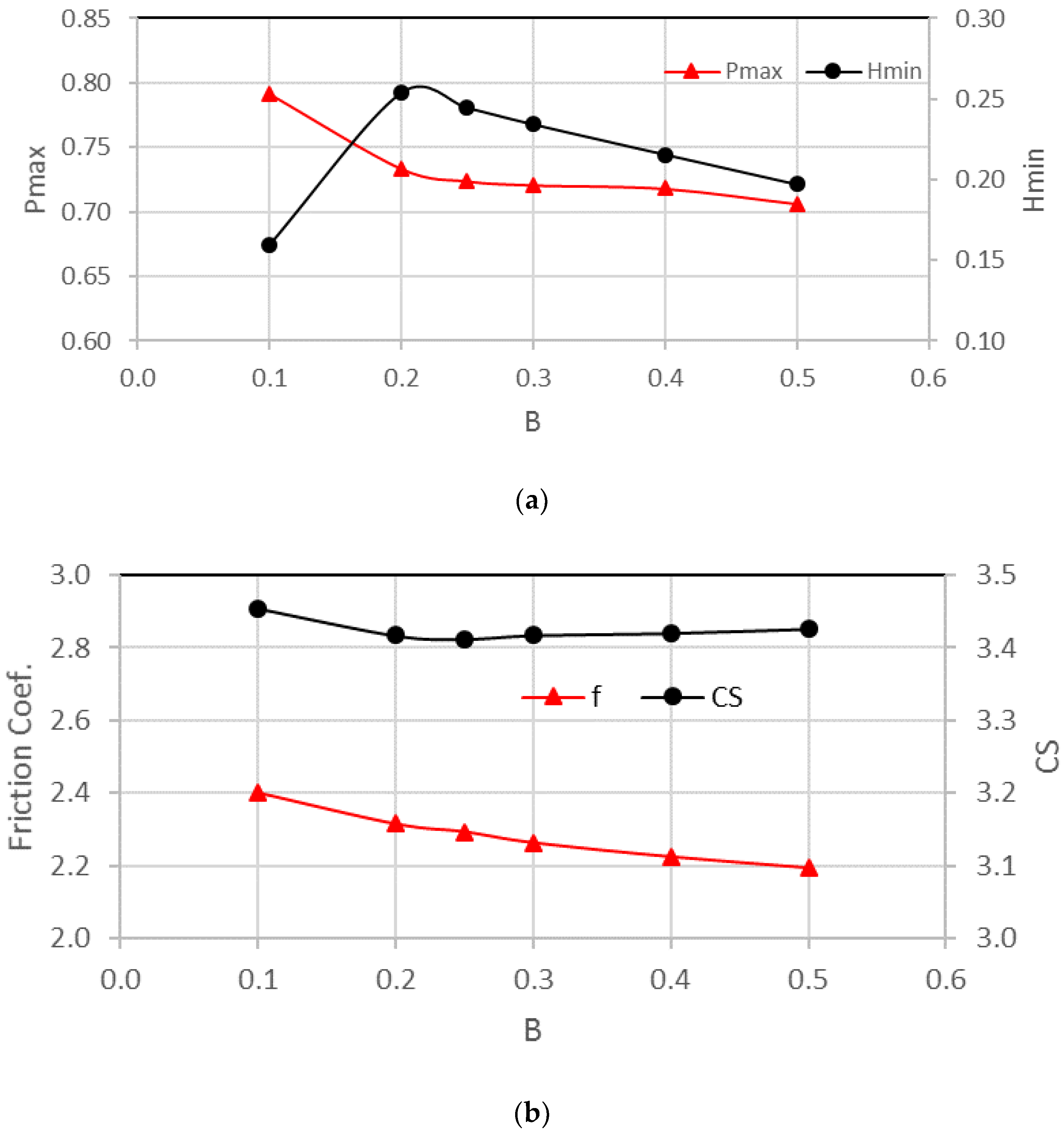
The effect of the chamfer parameter, $B$, which represents the amount of material removal from the bearing’s inner surface in the longitudinal direction of the bearing, is illustrated in Figure 11. Figure 11a represents the variation of $P_{max}$ and $H_{min}$ with $B$ and Figure 11b illustrates the corresponding variations in the friction coefficient and the critical speed. It can be seen that the optimum range of $B$ is $0.2\le B\le 0.4$ where the four examined characteristics responded more efficiently over this range. The other modification parameter, $A$, which represents the amount of material removal in the radial direction from the bearing inner surface, has also been examined in detail, where the optimum value is found to be 0.25.

The investigation of the bearing modification is further extended to include the time response of the journal to the position perturbation. If the journal shifts to the bearing center and is released, the resulting movement of its center reflects its stability characteristics. If the journal returns to its equilibrium position, this means that the rotor-bearing system is stable. On the other hand, for the critical case, the shaft is whirling around the equilibrium position. If the shaft rotates at a speed greater than its critical speed, the vibration amplitude will increase with time until it reaches the bearing wall. Therefore, the stability of the modified and unmodified bearings is examined in terms of the time response of the position coordinates $x$ and $y$ and the eccentricity ratio, ${\epsilon }_r$ under four operation speeds. The first speed is less than the critical speed of both modified and unmodified bearings, with the responses shown in Figure 12. It can be seen that the shaft center returns to its equilibrium position after a relatively short period of time $(t<0.1 \mathrm{s}),$ which means, in other words, that the system for both bearings is stable. 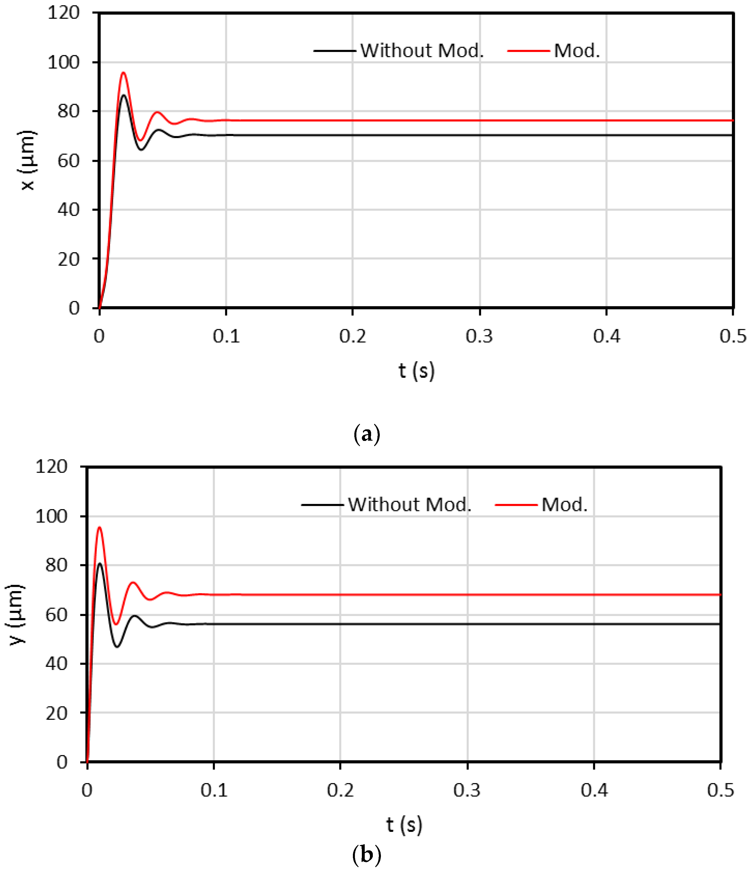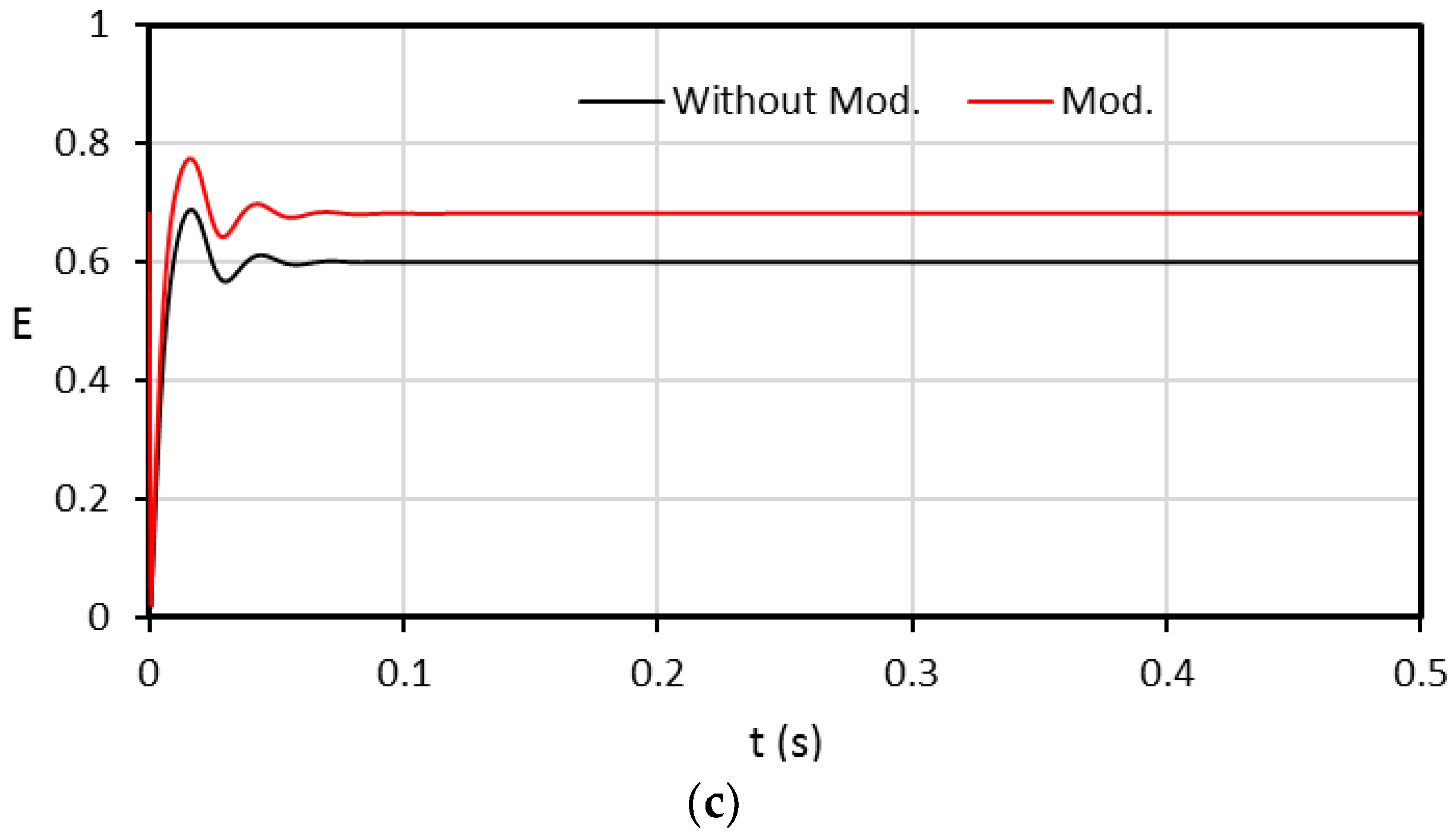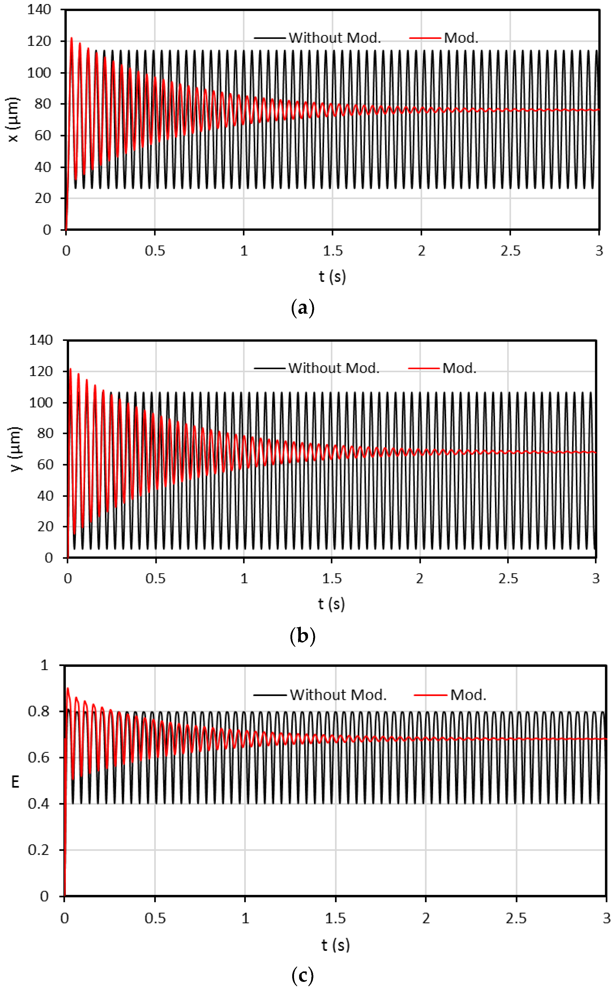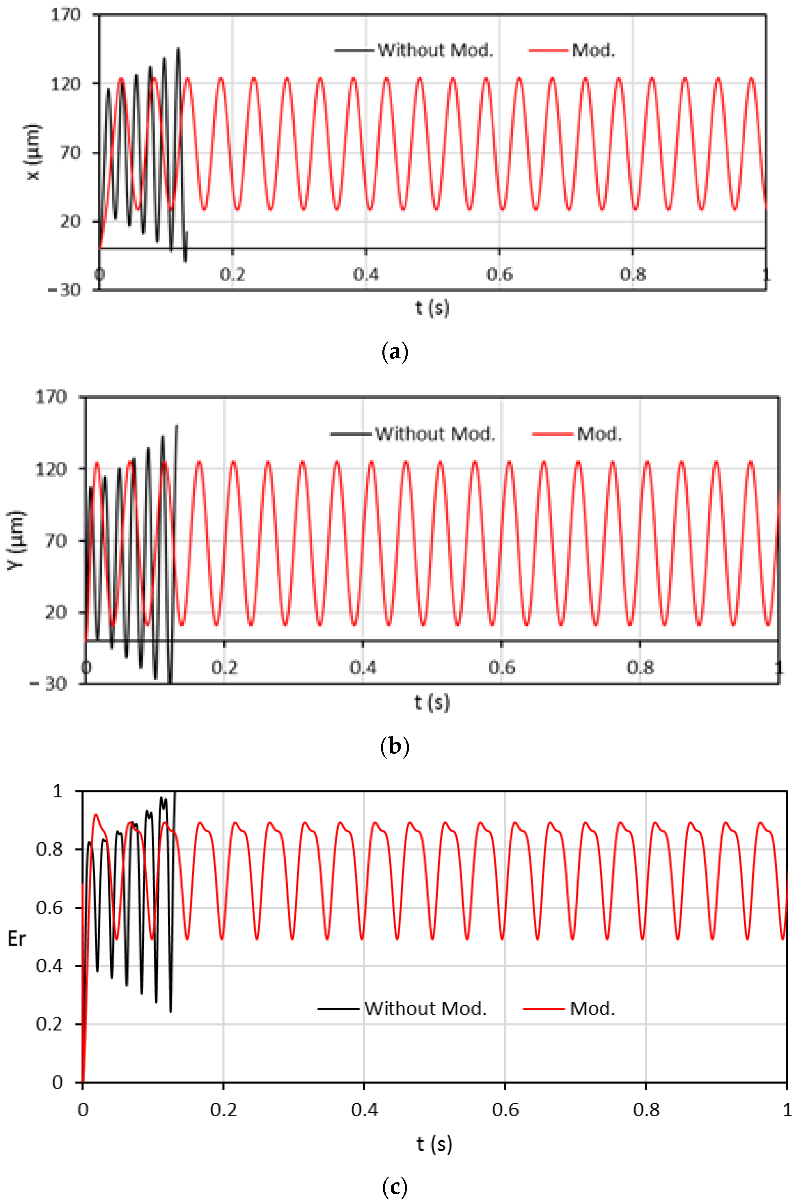Figure 13 illustrates the time responses when the journal rotates at a speed equal to the critical speed of the unmodified bearing. It can be seen that the modified bearing is stable as it returns to its equilibrium position after about 3 s while all the responses of the unmodified bearing repeated with time, which means that the bearing system is under a critical situation. The third chosen speed is the critical speed of the modified bearing, where the time responses under this operating speed are illustrated in Figure 14. It can be seen that when the $x$ and $y$ response of the unmodified bearing increased with time and exceeded 140 $\mathsf{\mu }\mathrm{m}$ when $t>0.1 \mathrm{s}$ (see Figure 14a,b) where the radial clearance used in this bearing is 150 $\mathsf{\mu }\mathrm{m}$. The combination of the $x$ and $y$ response gives the eccentricity ratio shown in Figure 14c, which is equal to 1 at t = 0.13 s, and which means that the journal surface touches the bearing wall. 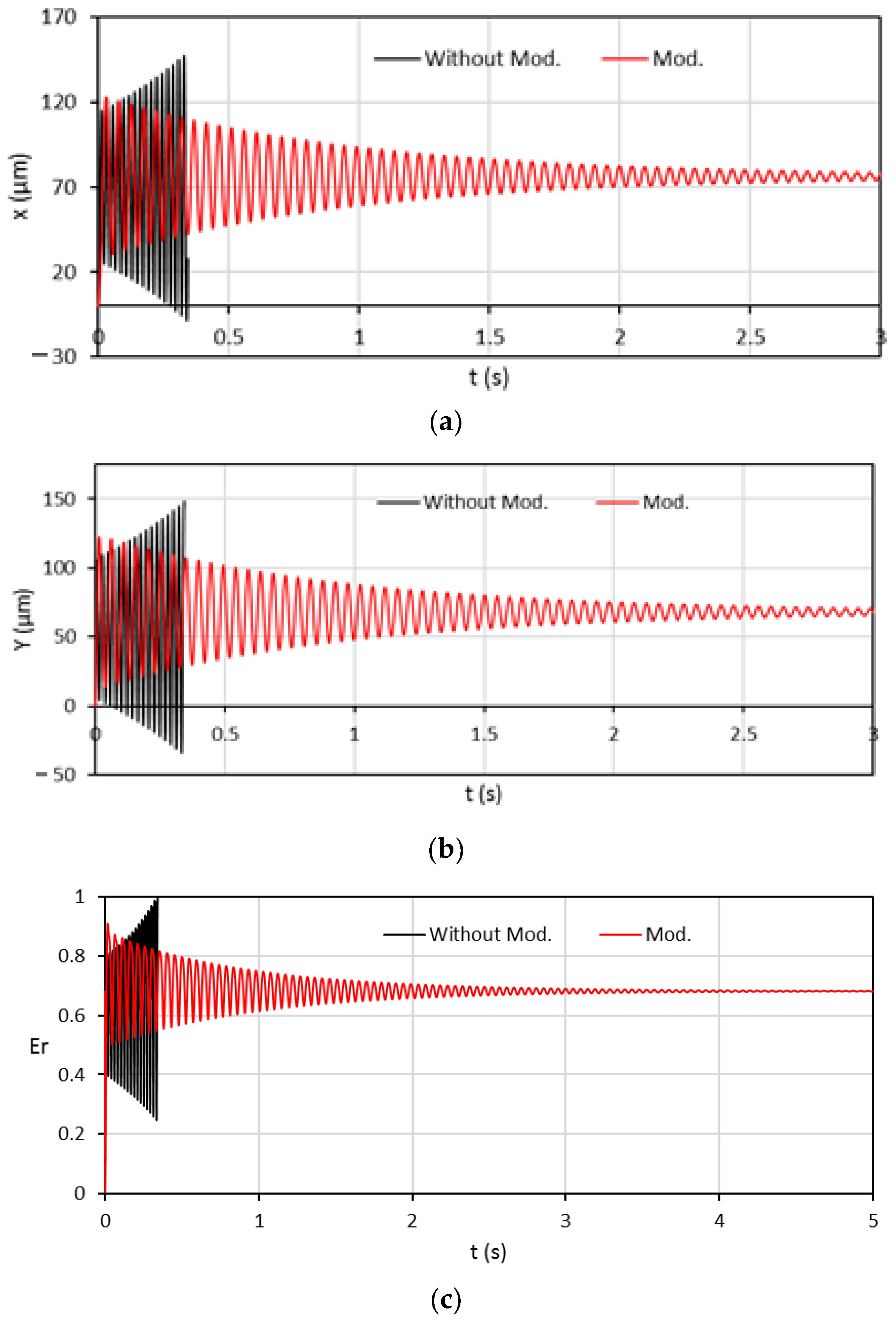On the other hand, the $x,y$, and ${\epsilon }_r$ responses of the modified bearing repeated with time as the bearing rotates at its critical speed. The last case shown in Figure 15 illustrates the responses when the operating speed is less than the critical speed of the modified bearing and greater than the critical speed of the unmodified bearing. It can also be seen that the modified bearing is stable, which requires about 5 s to return to its equilibrium position, while the unmodified bearing is unstable where the journal surface reaches the bearing wall after 0.33 s. It is clear that the modified bearing operates safely over a wider range of speeds compared to the unmodified bearing. It is worth mentioning that the time response of the misaligned and modified bearing is an extremely complex problem as it requires a solution for the equations of motion corresponding to geometry in space. However, this important solution will be addressed by the authors in the near future.

7. Conclusions

This paper presents a numerical solution for the problem of misaligned journal bearings, considering the misalignment in the vertical plane in addition to a general 3D misalignment case. The solution considers varying the bearing profile in order to reduce the misalignment effect and investigate the system time responses to the position perturbation. The solution considers the Reynolds boundary condition to identify the cavitation zone. It has been found that vertical misalignment has more negative consequences in terms of the maximum pressure and minimum film thickness values. The pressure distribution is much more asymmetrical compared to the 3D misalignment case. However, the 3D misalignment has many negative consequences on the coefficient of friction at the higher levels of misalignment, which increased by 15.6% in comparison with 6.92% for the vertical misalignment case. The variable profile of the bearing reduces $P_{max}$ by 26.6% 29.2% and reduces the friction coefficient by 4.97% and 9.76% for the vertical and 3D misalignment cases, respectively. The minimum film thickness in both cases of misalignment has increased almost three times, and the critical speed and the time responses are also improved by varying the bearing profile.

References

1. Jang, J.Y.; Khonsari, M.M. On the Characteristics of Misaligned Journal Bearings. Lubricants 2015, 3, 27–53. [Google Scholar] [CrossRef]
2. Girish, H.; Pai, R. Effect of journal misalignment on the static characteristics of an innovative journal bearing with adjustable elements in load-on-pad and load-between-pad configurations. Eng. Comput. 2021, 38, 1513–1531. [Google Scholar] [CrossRef]
3. Singh, D.V.; Sinhasan, R. Performance Characteristics of an Ungrooved Big-End Bearing with Misalignment. STLE Tribol. Trans. 1989, 32, 234–238. [Google Scholar] [CrossRef]
4. Choy, F.K.; Braun, M.J.; Hu, Y. Analytical and Numerical Study of a Misaligned Cavitating Hydrodynamic Cryogenic Journal Bearing. Tribol. Int. 1992, 25, 3–15. [Google Scholar] [CrossRef]
5. Nikolakopoulos, P.G.; Papadopoulos, C.A. Non-Linearities in Misaligned Journal Bearings. Tribol. Int. 1994, 27, 243–257. [Google Scholar] [CrossRef]
6. Ebrat, O.; Mourelatos, Z.P.; Vlahopoulos, N.; Vaidyanathan, K. Calculation of Journal Bearing Dynamic Characteristics Including Journal Misalignment and Bearing Structural Deformation©. Tribol. Trans. 2004, 47, 94–102. [Google Scholar] [CrossRef]
7. Sun, J.; Gui, C.L. Hydrodynamic lubrication analysis of journal bearing considering misalignment caused by shaft deformation. Tribol. Int. 2004, 37, 841–848. [Google Scholar] [CrossRef]
8. Jamali, H.; Al-Hamood, A. A New Method for the Analysis of Misaligned Journal Bearing. Tribol. Ind. 2018, 40, 213–224. [Google Scholar] [CrossRef]
9. Song, X.; Wu, W.; Yuan, S. Mixed-lubrication analysis of misaligned journal bearing considering turbulence and cavitation. AIP Adv. 2022, 12, 015213. [Google Scholar] [CrossRef]
10. Dufrane, K.F.; Kannel, J.W.; McCloskey, T.H. Wear of steam turbine journal bearings at low operating speeds. J. Lubr. Technol. 1983, 105, 313–317. [Google Scholar] [CrossRef]
11. Bouyer, J.; Fillon, M. An experimental analysis of misalignment effects on hydrodynamic plain journal bearing performances. J. Tribol. 2002, 124, 313–319. [Google Scholar] [CrossRef]
12. Sun, J.; Gui, C.; Li, Z. An experimental study of journal bearing lubrication effected by journal misalignment as a result of shaft deformation under load. J. Tribol. 2005, 127, 813–819. [Google Scholar] [CrossRef]
13. Nikolakopoulos, P.G.; Papadopoulos, C.A. A study of friction in worn misaligned journal bearings under severe hydrodynamic lubrication. Tribol. Int. 2008, 41, 461–472. [Google Scholar] [CrossRef]
14. Nacy, S.M. Effect of Chamfering on Side-Leakage Flow Rate of Journal Bearings. Wear 1997, 212, 95–102. [Google Scholar] [CrossRef]
15. Fillon, M.; Bouyer, J. Thermohydrodynamic Analysis of a Worn Plain Journal Bearing. Tribol. Int. 2004, 37, 129–136. [Google Scholar] [CrossRef]
16. Strzelecki, S. Operating Characteristics of Heavy Loaded Cylindrical Journal Bearing with Variable Axial Profile. Mater. Res. 2005, 8, 481–486. [Google Scholar] [CrossRef]
17. Chasalevris, A.; Dohnal, F. Enhancing Stability of Industrial Turbines Using Adjustable Partial Arc Bearings. J. Phys. 2016, 744, 012152. [Google Scholar] [CrossRef]
18. Ren, P.; Zuo, Z.; Huang, W. Effects of axial profile on the main bearing performance of internal combustion engine and its optimization using multiobjective optimization algorithms. J. Mech. Sci. Technol. 2021, 35, 3519–3531. [Google Scholar] [CrossRef]
19. Jamali, H.U.; Sultan, H.S.; Abdullah, O.I.; Al-Tamimi, A.N.J.; Albdeiri, M.S.; Ruggiero, A.; AL-Dujaili, Z.A. Analysis of the Performance of Chamfered Finite-Length Journal Bearings under Dynamic Loads. Mathematics 2023, 11, 587. [Google Scholar] [CrossRef]
20. Jamali, H.U.; Sultan, H.S.; Abdullah, O.I.; Al-Tamimi, A.N.J.; Abbud, L.H.; Ruggiero, A.; Al-Dujaili, Z.A. Effect of Chamfer Form and Parameters on the Characteristics of Finite Length Journal Bearing under Impact Load. Lubricants 2023, 11, 73. [Google Scholar] [CrossRef]
21. Allmaier, H.; Offner, G. Current Challenges and Frontiers for the EHD Simulation of Journal Bearings: A Review; SAE Technical Paper 2016-01-1856; SAE: Warrendale, PA, USA, 2016. [Google Scholar] [CrossRef]
22. Chasalevris, A.; Sfyris, D. Evaluation of the Finite Journal Bearing Characteristics, Using the Exact Analytical Solution of the Reynolds Equation. Tribol. Int. 2013, 57, 216–234. [Google Scholar] [CrossRef]
23. Hamrock, B.J. Fundamentals of Fluid Film Lubrication; McGraw-Hill, Inc.: New York, NY, USA, 1991. [Google Scholar]
24. Harnoy, A. Bearing Design in Machinery: Engineering Tribology and Lubrication, 1st ed.; Marcel Dekker Inc.: New York, NY, USA; Basel, Switzerland, 2002. [Google Scholar]
25. Feng, H.; Jiang, S.; Ji, A. Investigation of the Static and Dynamic Characteristics of Water-Lubricated Hydrodynamic Journal Bearing Considering Turbulent, Thermo-hydrodynamic and Misaligned Effects. Tribol. Int. 2019, 130, 245–260. [Google Scholar] [CrossRef]
26. Lund, J.W.; Thomsen, K.K. A Calculation Method and Data for the Dynamic Coefficients of Oil-Lubricated Journal Bearings; ASME: New York, NY, USA, 1978. [Google Scholar]
27. Someya, T. Journal Bearing Databook; Springer: Berlin/Heidelberg, Germany, 1989. [Google Scholar]
28. Tieu, A.K.; Qiu, Z.L. Stability of Finite Journal Bearings -from Linear and Nonlinear Bearing Forces. Tribol. Trans. 1995, 38, 627–635. [Google Scholar] [CrossRef]
29. Shi, Y.; Li, M.; Li, M. Study on nonlinear dynamics of the marine rotor-bearing system under yawing motion. J. Phys. Conf. Ser. 2020, 1676, 012156. [Google Scholar] [CrossRef]
30. D’Amato, R.; Amato, G.; Wang, C.; Ruggiero, A. A Novel Tracking Control Strategy with Adaptive Noise Cancellation for Flexible Rotor Trajectories in Lubricated Bearings. IEEE/ASME Trans. Mechatron. 2021, 27, 753–765. [Google Scholar] [CrossRef]
31. Nicholas, J.C. Hydrodynamic Journal Bearings-Types, Characteristics and Applications; Rotating Machinery Technology, Inc.: Wellsville, NY, USA, 1996. [Google Scholar]
Figure 1. Schematic drawing of the solution model. (a) Side view of the journal bearing, (b) 3D aligned journal bearing, (c) general 3D mis. model, and (d) bearing profile mod [20].
Lubricants 11 00173 g001aLubricants 11 00173 g001b
Figure 2. Schematic drawing of: (a) journal bearing, (b) rotor [29] edited.
Lubricants 11 00173 g002
Figure 3. Flowchart of the solution procedure (edited from [20]).
Lubricants 11 00173 g003
Figure 4. Dimensionless results of the perfectly aligned bearing, (a) Pressure distribution and (b) film thickness.
Lubricants 11 00173 g004
Figure 5. Effect of the form of misalignment on the dimensionless pressure distribution. Left: Vertical and Right: 3D misalignments. (a) Mis. Parameter = 0.2; (b) Mis. Parameter = 0.5; (c) Mis. Parameter = 0.55; (d) Mis. Parameter = 0.57; (e) Mis. Parameter = 0.59.
Lubricants 11 00173 g005aLubricants 11 00173 g005bLubricants 11 00173 g005c
Figure 6. Effect of varying bearing profile on the dimensionless pressure distribution. (a) Vertical and (b) 3D misalignment. Left: unmodified and right: modified profile.
Lubricants 11 00173 g006
Figure 7. Effect of varying bearing profile on the dimensionless film thickness distribution. (a) Vertical and (b) 3D misalignment. Left: unmodified and right: modified profile.
Lubricants 11 00173 g007
Figure 8. Effect of the dimensionless misalignment parameters for the two cases of misalignment (vertical and 3D) on the dimensionless: (a) Pmax and Hmin and (b) friction coefficient and critical speed.
Lubricants 11 00173 g008
Figure 9. Effect of profile modification (vertical misalignment) on the dimensionless: (a) Pmax and Hmin and (b) friction coefficient and critical speed. A = B = 0.25 .
Lubricants 11 00173 g009
Figure 10. Effect of profile modification (3D misalignment) on the dimensionless: (a) Pmax and Hmin and (b) friction coefficient and critical speed. A = B = 0.25 .
Lubricants 11 00173 g010
Figure 11. Effect of the dimensionless profile parameter B for the case of 3D misalignment on the dimensionless: (a) Pmax and Hmin and (b) friction coefficient and critical speed. A = 0.25 .
Lubricants 11 00173 g011
Figure 12. Time response to position perturbation of the rotor bearing system for modified and unmodified profile under a rotational speed less than the critical speed of the unmodified bearing: (a) x(t), (b) y(t), and (c) eccentricity ratio as a function of time.
Lubricants 11 00173 g012aLubricants 11 00173 g012b
Figure 13. Time response to position perturbation of the rotor bearing system for modified and unmodified profile under a rotational speed equal to the critical speed of the unmodified bearing: (a) x(t), (b) y(t), and (c) eccentricity ratio as a function of time.
Lubricants 11 00173 g013
Figure 14. Time response to position perturbation of the rotor bearing system for modified and unmodified profile under a rotational speed equal to the critical speed of the modified bearing: (a) x(t), (b) y(t) and (c) eccentricity ratio as a function of time.
Lubricants 11 00173 g014
Figure 15. Time response to position perturbation of the rotor bearing system for modified and unmodified profile under a rotational speed greater than the critical speed of the unmodified bearing: (a) x(t), (b) y(t), and (c) eccentricity ratio as a function of time.
Lubricants 11 00173 g015