1. Introduction
With the wide application of pulse width modulation inverters in motors, bearing current damage has become an important concern for high-power motors. When the motor is running, due to the fast change of the frequency of the variable frequency drive and the high pulse voltage, it is easy to generate the threshold voltage of the lubricating oil film at both ends of the shaft, which exceeds the threshold voltage of the bearing, and the tip discharge occurs on the contact surface between the bearing raceway and the rolling element, causing the shaft current damage and causing safety accidents. In high-end equipment, such as high-speed rail trains, large wind turbines, and new energy buses, the power of the generators and motors is increasing, the frequency conversion control system is becoming more and more complex, and the bearing current damage is increasing, resulting in a sharp reduction in the life of the batch bearings relative to the design life. At present, the monitored bearing fault signal is often misjudged as ordinary fatigue wear or other mechanical damage. Simply replacing the bearing without taking electrical insulation maintenance measures is palliative. If the fault type of the motor bearing cannot be accurately identified, the same fault type will repeatedly appear, delaying the best maintenance time of the motor system, causing huge safety hazards and economic losses. Therefore, the accurate identification of motor bearing faults is crucial [
1].
At present, there are much research on the current damage of motor bearings, including the mechanism and key influencing parameters of the bearing current, the circuit model of the bearing current and the damage to the bearing performance [
2,
3]. Chen et al. [
4] proposed corresponding improvement measures for the wind turbine mechanism in view of the problem of shaft voltage and shaft current of the wind turbine. Xu et al. [
5] analyzed the mechanism of shaft current generation and the method of shaft current suppression in a hydro-generator. Adabi et al. [
6] analyzed the causes of the shaft voltage of induction generator and proposed the suppression measures of the shaft current. Some scholars have studied the generation mechanism and damage characteristics of shaft voltage and shaft current from an electrical point of view for specific generators and motors. For example, Prashad et al. [
7] established a charge accumulation and discharge energy model with the time period, corrosion pit size, and bearing capacitance as the parameters, so as to determine the shaft voltage and diagnose the bearing failure caused by corrosion pits. Liu et al. [
8] analyzed the electrical discharge machining, wrinkling, and its characterization caused by bearing current from the perspective of tribology. Picot assumed that the premature failure of the bearing was caused by the high-frequency current passing through the bearing. A Weibull cycle statistical method based on the stator current was proposed to construct a stable, normalized fault index [
9]. Liu et al. [
10,
11] established an equivalent electrical model of the bearing, simulated the process of the bearing breakdown and recovery, and proposed measures to suppress the bearing current of small generators and motors. There are also scholars from the statistical point of view using current monitoring data and vibration monitoring data to establish the identification model of bearing current damage and detect fault in bearing current damage. For example, Kempski proposed an electrostatic discharge statistical model of induction motor bearings generated by inverters, which can be used as a research basis for bearing damage risk of different drive devices [
12]. Houssin proposed a stator current parameter spectrum estimation method to detect induction motor bearing faults. The effectiveness of bearing fault detection is verified by simulation analysis [
13]. Based on a collaborative filtering algorithm and manifold learning algorithm, Wang et al. [
14,
15] studied the fault identification and state prediction of bearing current damage. Chen et al. [
16] proposed a lifting wavelet fractal strategy to extract the impact fault features reflecting bearing faults from multi-component coupled vibration signals, which has a more comprehensive ability to analyze the current damage characteristics of motor bearings. Through the above literature review, it is clear that the problem of motor bearing current damage is common in high-power motors. The research on current damage mechanism, current suppression method, and current fault detection have always been a hot spot. However, most of the current research on the current damage of motor bearings summarize and analyze the causes of bearing current from the results of shaft current damage or establish a corresponding equivalent physical model to simulate the process of bearing damage. These research methods have high diagnostic accuracy for motor bearing current damage, but their applicability is not wide, and the cost is high. There are also some studies based on data, but in the study of bearing current damage, bearing current damage is greatly affected by factors such as motor speed [
17,
18,
19], load [
20], and grease [
21,
22]. Different working conditions will lead to different data distribution, thus greatly reducing the efficiency of the fault diagnosis [
23].
The traditional data-driven rolling bearing fault diagnosis method requires two basic premises: the distribution of the training data and test data is the same; there are enough available training samples [
24]. In view of the need for a large number of samples, many studies have effectively alleviated the problem of insufficient numbers of labeled samples through the construction of semi-supervised learning frameworks [
25,
26]. The same distribution of data requires the same environmental conditions when collecting the bearing vibration signals. In the context of the Internet of Things and big data, most machine learning will collect data in various parts of the machine that may fail [
27] and will train multiple fault diagnosis models. This method can also solve the problem of different data distributions, but it will consume huge manpower and material resources and is expensive. The transfer learning emerges as the time requires. The transfer of existing knowledge solves the learning problems that are difficult to obtain for the label samples in the target domain. The method of applying the knowledge learned in a domain (source domain) to different but related domains (target domain) is called transfer learning [
28]. Transfer learning also has many applications in the field of bearing fault diagnosis [
29,
30,
31]. Considering that the bearing vibration data under variable working conditions will have similar fault characteristics, minimizing the cross-domain distribution distance has become a hot issue to be solved in the field of bearing fault diagnosis. Lan et al. [
32] proposed a cross-domain bearing fault classification method based on transfer component analysis (TCA), which significantly reduces the inter-domain distribution distance by minimizing the maximum mean difference between the source domain and the target domain and achieves cross-domain edge distribution alignment. The manifold embedded distribution alignment (MEDA) method is a transfer manifold learning method with dynamic distribution adaptability, proposed by Wang et al. [
33] on the basis of joint distribution adaptation (JDA) [
34], which achieves better domain adaptation by quantitatively evaluating the relative importance of the edge distribution and conditional distribution. Zhang et al. [
35] proposed a small sample bearing fault diagnosis method based on transfer learning, using a sufficient number of the source domain samples to train the network to prevent network overfitting, and using 1% of the target domain training set data to fine-tune the model classification ability. Zhao et al. [
36] used bidirectional gated recurrent units to generate auxiliary samples for the source domain of MEDA, so that excellent fault identification can be maintained in the case of a small number of labeled samples.
However, the above research focuses on the alignment of the edge distribution and the conditional distribution. As a cross-domain alignment, these two distribution alignments ignore the internal structure information of the domain, and the shaft current damage characteristics of the motor bearing and the common fault characteristics are easily confused, resulting in category overlap in the domain. In view of the internal structure of the field, many scholars have applied metric learning to better learn the distance or similarity between samples. By changing the original sample distribution, the intra-class dispersion and inter-class similarity are reduced, and the recognition ability of the classifier is improved [
37]. Xu et al. [
38] combined transfer learning with metric learning to improve the accuracy of the fault feature clustering by minimizing the correlation alignment loss, narrowing the distribution difference between the source domain and the target domain, and maximizing the similarity between the input feature and the center feature. Zhao et al. [
39] used triplet loss to measure the distance between various faults, so that the distance between similar fault features is very small, and the distance between heterogeneous fault features is very large. However, the above deep metric transfer learning applied to bearing fault diagnosis focuses on the Euclidean distance between the classes in the alienation domain, which leads to the neglect of spatial cross-domain tilt and manifold structure mining. As the acquisition of the equipment status information becomes more and more difficult, the amount of fault data is small, and it is impossible to effectively label all working condition data, so the label samples are very precious [
40]. In order to make efficient use of the existing fault data and fully exploit the manifold similarity between data under the diversity, time-varying, and strong nonlinearity of the working conditions, it is very important to pay attention to cross-domain tilt and intra-domain alienation.
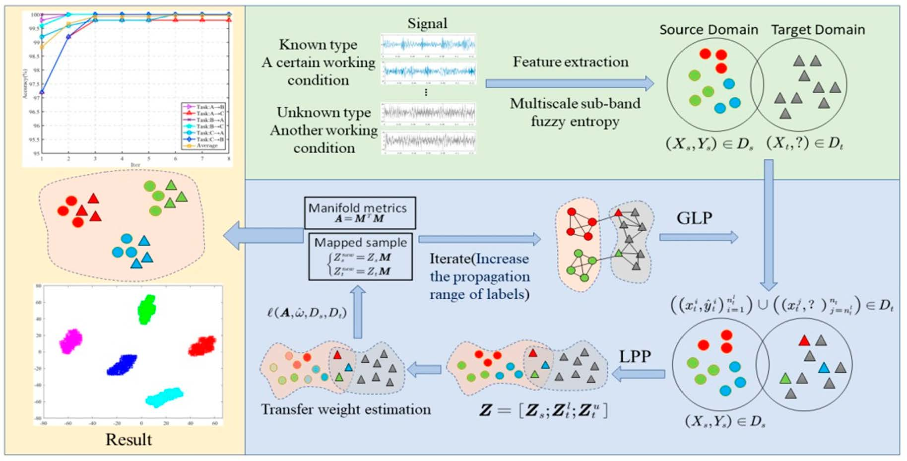
In view of the extreme service environment and complex working load of motor bearing, the damage state signal of motor bearing presents the characteristics of weak and nonlinear and is often submerged in strong background noise and interference signal. Its common features are difficult to fully characterize as the shaft current damage of motor bearing, and the recognition effect under variable working conditions is poor. A method of shaft current damage identification of motor bearing under variable working conditions based on multiscale feature label propagation and manifold metric transfer is proposed. Firstly, the sensitive feature set of bearing current damage is constructed by extracting the multiscale sub-band fuzzy entropy features of the signal, which can better identify the bearing current damage. Then, according to the proposed features, the weighted graph is constructed on the source domain of the known fault label, and the source domain label information is gradually diffused by graph label propagation, which solves the limitation that the semi-supervised metric transfer learning needs supervised samples. At the same time, the LPP algorithm is used to map the multiscale sub-band fuzzy entropy of the sample to the low-dimensional manifold space, and the manifold distance metric is learned to align the source domain and the target domain. The intra-class distance is minimized, and the inter-class distance is maximized to eliminate the overlap in the domain and realize unsupervised metric transfer learning. In the case of no target domain label samples, the problem of poor bearing current damage identification under different working conditions is solved. The proposed method mainly has the following four advantages: (1) This method belongs to the unsupervised transfer learning method, which breaks the limitation that the traditional metric transfer learning needs the target domain sample label. (2) This method considers the manifold relationship between data samples, mining the manifold structure between data. (3) The proposed method takes into account the problems of domain tilt, excessive inter-domain distance, and intra-domain overlap, which are neglected in the current damage identification of motor bearing shaft under variable working conditions. (4) The multiscale sub-band fuzzy entropy extracted by this method can dig deep into the essential information of the vibration information and can accurately identify the current damage fault of the motor bearing.
2. Multiscale Sub-Band Fuzzy Entropy and Metric Transfer Theory
2.1. Multiscale Sub-Band Fuzzy Entropy
Fuzzy entropy is a measure of the complexity of time series. It describes the information contained in time series samples more accurately by introducing the fuzzy membership function. However, when the sequence is too complex, the ordinary fuzzy entropy extraction cannot dig deep into the internal information of the data. In order to solve this problem, we put forward the concept of multiscale sub-band fuzzy entropy. Firstly, the signal is decomposed into multiscale sub-band signals by wavelet packet, and, finally, the fuzzy entropy of each multiscale sub-band signal is obtained. Because this method can go deep into the data and decompose and mine the eigenvalues and eigenvectors of the data layer by layer, it can effectively and accurately extract the fault features of complex weak data. The specific steps of multiscale sub-band fuzzy entropy are:
(1) The vibration signal is decomposed and reconstructed by layer wavelet packets, and wavelet packet decompositions and reconstruction sequences are obtained. is the th sub-band sequence of the layer decomposition of signal by the wavelet packet.
(2) Taking the sub-band
as an example, given the dimension
, the sub-band signal
is composed of a set of
dimensional vectors, according to the serial number, namely:
where
and
is the length of the sub-band sequence.
(3) The distance is calculated between each sequence and the remaining sequences
:
where
(4) Given a threshold
(
is the standard deviation of the original data), ambiguity
, through the fuzzy membership function
, the distance matrix is redefined:
(5) The average of all memberships is found:
(6) The dimension is increased to , steps (2)–(5) are repeated to obtain .
(7) The fuzzy entropy of
is:
(8) Steps (2)–(7) are repeated and the fuzzy entropy of sub-band , respectively, is calculated.
(9) In this paper, the sub-band sequences
are calculated, respectively, and the characteristic matrix is constructed. The multiscale sub-band fuzzy entropy of the fault signal is
:
2.2. Metric Transfer Learning
Metric learning can adaptively learn metrics from raw data with the same distribution, change the distribution of the original samples, reduce the distance between similar samples, and dissimilate heterogeneous samples to greatly improve the efficiency of machine learning. Metric transfer learning reduces the difference of the sample distribution caused by different data distributions and maintains better classification ability when data are distributed differently.
For a given sample set
, the core goal of metric learning is to find an optimal learning metric
, under which the samples of the same class are more aggregated in space and alienated into different classes. Therefore, Jin et al. formulated the following regular objective functions [
41]:
where
is a positive semidefinite matrix;
denotes the loss function;
is the indicator matrix within and between classes. When two samples are of the same class,
, otherwise
.
According to the above objective function, a distance metric
can be obtained. Under this metric, the distance between sample
and sample
can be expressed as:
Traditional distance metric learning is based on the premise that all samples obey the same distribution. When the distribution of samples in the space is inconsistent, the effect of metric learning will decline or even fail. Therefore, after the metric transfer learning [
42] introduces sample cross-domain information in the metric learning, the loss function becomes:
where
is the sample weight;
and
represent the loss functions within and between classes. The specific expressions are as follows:
Metric transfer learning solves the domain offset problem by assigning different weights to the labelled samples, and clustering and alienating samples in the field on the basis of cross-domain alignment, and maximizes the class spacing to obtain the distance metric .
3. Label Propagation and Manifold Metric Transfer Learning Algorithm
Due to the difference of spatial distribution between the source domain and the target domain, simple feature normalization in the domain cannot solve the problems of domain offset and domain tilt. When the number of source domain samples of known labels is scarce, the effect of the source domain and the target domain alignment often decreases greatly, and the existing transfer learning methods pay more attention to the overall cross-domain alignment of the domain and less attention to the distribution within the domain. In the motor bearing shaft current damage identification, the similar features between the shaft current damage and ordinary fault leads to different types of overlap. Many machine learnings directly measure the similarity between data in the original Euclidean space, ignoring the hidden manifold structure relationships in the sample space. Therefore, in order to mine the manifold similarity between data, pay attention to the structural information between and within the domain, and get rid of the dependence on the label samples of the target working condition. An unsupervised transfer learning method based on multiscale feature label propagation and manifold metric transfer is proposed, aiming at eliminating the domain overlap and intra-domain overlap in the manifold space.
3.1. Graph-Based Label Propagation
The core idea of graph-based label propagation (GLP) is that similar samples will have similar label graphs. Label propagation propagates samples with known labels to predict unknown labels through connected edges [
43]. Commonly used graphs have weighted graphs. Each sample can be regarded as a node. The connection weight of Node
and Node
can be expressed as:
where
represents the
nearest neighbor set of point
. The loss function of cross-domain label propagation from the source domain to the target domain is defined as follows:
where,
is the label matrix of the source domain
.
is the label matrix of the target domain, and the same value is initialized.
represents the Laplace matrix of the graph,
is a diagonal matrix, and its diagonal elements are the sum of the column elements of the
matrix.
The label matrix of the target domain can be obtained by minimizing the loss function of label propagation. Because the target domain does not provide the supervision information of labels, there are errors in cross-domain label propagation, and then we gradually reduce the label errors by iterative method.
3.2. Locality Preserving Projections
In the original space, the sample distribution is different because of the different data acquisition environment between the source domain and the target domain. Many machine learning methods use Euclidean distance to measure the similarity between samples or transfer the source domain and the target domain directly in Euclidean space, which do not consider that the nonlinear manifold structure between the samples may not achieve the ideal transfer effect. Therefore, we use the locality preserving projection in manifold learning to mine the hidden manifold structure in Euclidean space and to find the similarity between samples, which is difficult to obtain.
The LPP algorithm [
44] breaks the limitation of traditional methods such as PCA, which have difficulty in mining the nonlinear manifold of data and can obtain low-dimensional projection more easily. LPP is also a graph-based manifold learning method. For the data set
in the original space, let
be the data in the original space and map it to the data in the low-dimensional manifold. By constructing a weighted graph
of the sample, the connected points in the weighted graph remain connected after the manifold mapping, and the error is minimized as the objective function:
The objective function is simplified:
where
is a diagonal matrix whose diagonal elements are the sum of the corresponding column elements in
.
By adding constraint
, the target function is converted to:
The optimization problem of the above formula is solved according to Lagrange multiplier method, which solves the eigenvalue and eigenvector problems of the generalized eigenequation of the following formula [
45]:
The transformation matrix is composed of eigenvectors corresponding to the first minimum eigenvalues of the above formula.
3.3. Label Propagation and Manifold Metric Transfer Learning
The label propagation and manifold metric transfer learning aims to find a manifold distance metric that can make the same kind of samples more clustered and the different kind of samples more dispersed in the domain, with the smallest inter-domain offset by label diffusion and metric learning on the graph of low-dimensional manifolds.
3.3.1. Cross-Domain Alignment Based on GLP
Because of the differences in the spatial distribution of data samples, there will be differences in similarity between the source domain samples and the target domain samples. We first map the samples in the original space to the low-dimensional manifold space and then give higher weights to the samples similar to the source domain and the target domain, which cannot only minimize the cross-domain manifold distance but also eliminate the cross-domain tilt phenomenon. Firstly, the prior weight of all labelled samples in the source domain is assumed to be
, and then a more accurate source domain sample weight
is obtained by introducing a regularization term to minimize the difference between the source domain and the target domain. The regularization term is expressed as:
where
is the density ratio estimation of the source domain sample
, which is used to express the weight of the samples in the cross-domain transfer. The higher the value of
, the more similar the source domain sample
is to the target domain sample, and the more important it is to measure the cross-domain manifold distance.
We use the method in reference [
46] to estimate the density ratio of samples in the source domain. The density ratio can be approximately considered as a combination of some basic linear functions:
where
represents a predefined Gaussian kernel function;
is the parameter corresponding to the basis function. Because different basis function
settings will affect the result of the density ratio estimation, sample
is selected from the target domain as the center of the Gaussian function (these samples are selected by GLP). The basis function
of Gaussian kernel is:
Therefore, the weight of the source domain samples can be solved by minimizing the KL-divergence between and .
According to the above, it can be summarized as the following optimization objectives:
For the above convex optimization problem, we can obtain the optimal solution by the gradient convergence method.
In the above formula, the cross-domain transfer weights
of all samples in the source domain are obtained. In order to make the source domain samples with high weight as close to the target domain as possible, semi-supervised metric transfer learning usually requires providing some supervised samples in the target domain. We select the supervised samples based on the GLP method, estimate the reconstruction density ratio
to
, and give the target domain samples a weight of 100%:
where
denotes a subset of samples learned according to the auxiliary metrics selected in the target domain, whose labels are pseudo labels.
3.3.2. Optimization Goal of Intra-Domain Alienation
In order to fully explore the similarity between the sample data in manifold space and LPP, a manifold mapping method is used based on the graph. Therefore, we introduce a regularization term
of graph:
where
,
is the diagonal matrix of the graph matrix
.
Combined with metric learning, we can obtain the following overall optimization goals:
where
is the indicator matrix within and between classes:
In order to solve the optimization problem of the objective function, it is necessary to converge
and
while satisfying constraints
, so the Lagrange multiplier is introduced to transform the objective function into:
where
is the label field indication matrix for distinguishing the selected samples of the source domain and the target domain:
The objective function obtains partial derivatives of
and
, respectively:
where
, sign is a symbolic function.
The values of
and
are then alternately updated using a gradient descent to obtain the cross-domain manifold distance metric
when the convergence condition, Formula (32), of the formula is satisfied.
Because the distance metric
is a positive semidefinite matrix, we can decompose
. For simplicity, the distance between sample
and sample
can be expressed as:
Under this manifold distance measure, it can be regarded that the samples after the LPP dimension reduction are mapped to a common subspace in the manifold space, where the sample distribution data in this space has the smallest cross-domain distance and the smallest cross-domain tilt, and the alienation between the clusters of the same class in the domain is obvious:
4. Shaft Current Damage Mechanism and Vibration Signal Characteristics of Motor Bearings
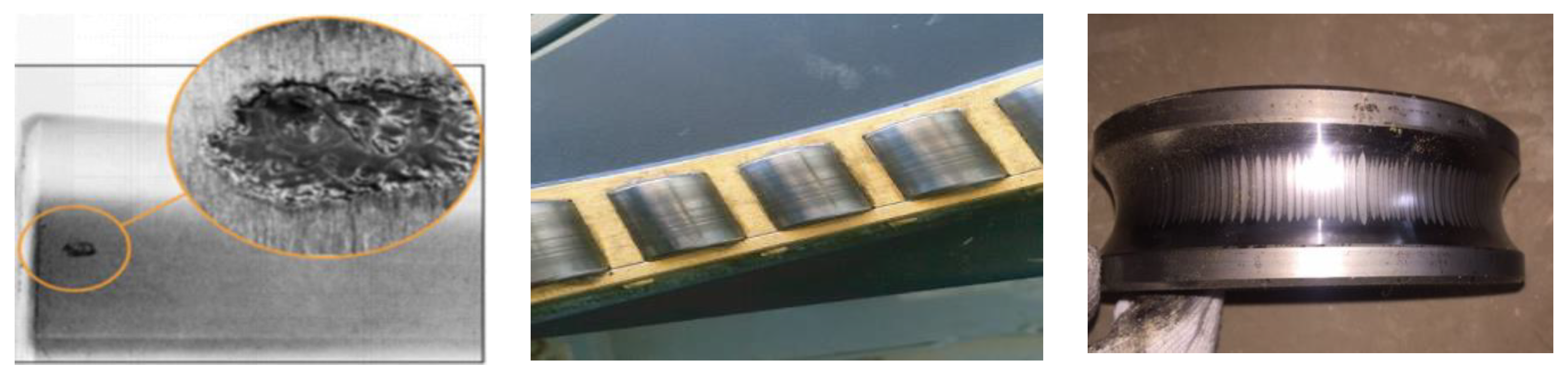
During the normal operation of the high-power motor, there is a lubricating oil film between the bearing rolling element and the raceway, which plays an insulating role. Both ends of the spindle will only produce a lower shaft voltage. When there are problems in the design and adjustment of the motor, the failure of the electrical system makes the shaft voltage increase, the insulation oil film between the bearings is destroyed, or the stable lubricating oil film is not formed in the bearing when the motor is just started, the electric potential difference between the inner and outer rings of the bearing exceeds the breakdown voltage that the lubricating oil film can withstand; the shaft voltage can easily break the oil film and discharge, resulting in shaft current. Because the contact point between the bearing raceway and the rolling element metal is very small, the skin effect phenomenon is generated on the surface of the bearing raceway, so the current density of these points increases, and the high temperature is instantaneously generated, so that the local melting or gasification of the bearing is caused. The molten bearing metal particles splash on the surface of the bearing raceway due to the radial load grinding pressure, so that the electric erosion occurs on the bearing ball and the raceway, resulting in small pits and pitting. Under the combined action of the current and mechanical load, the electric erosion area of the bearing continues to expand, and a typical bearing current damage morphology of a ‘washboard‘ shape is gradually formed, as shown in
Figure 1.
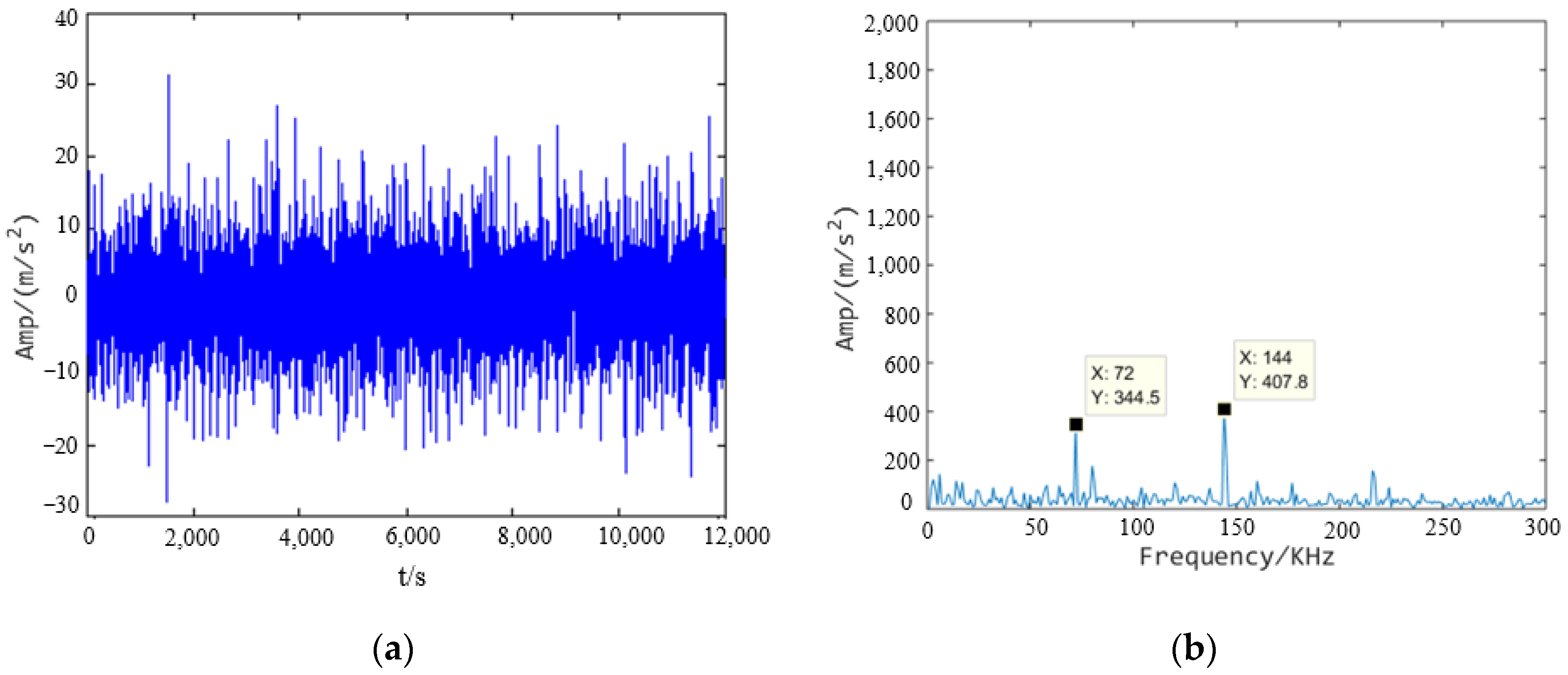
According to the principle of shaft current damage of bearing, the bearing current damage experiment is carried out by using the bearing current damage test bench. The programmable current source intermittently loads the current of the experimental bearing, continuously loads the current of 2 A for 15 min, stops the current loading in the next 5 min, and so on. The rotational speed used in the bearing current damage experiment is 1200 rpm and the load size is constant at 1000 N. The experimental bearing is a 6205 deep-groove ball bearing with an inner diameter of 52 mm, an outer diameter of 25 mm, and with 9 balls. The characteristic frequency of the outer ring fault is fo = 71.7 Hz, the characteristic frequency of the inner ring fault is fi = 108.3 Hz, and the characteristic frequency of the rolling element fault is fb = 47.17 Hz. The time domain diagram and envelope spectrum of the vibration signal of the shaft current damage bearing in different time periods are shown in
Figure 2,
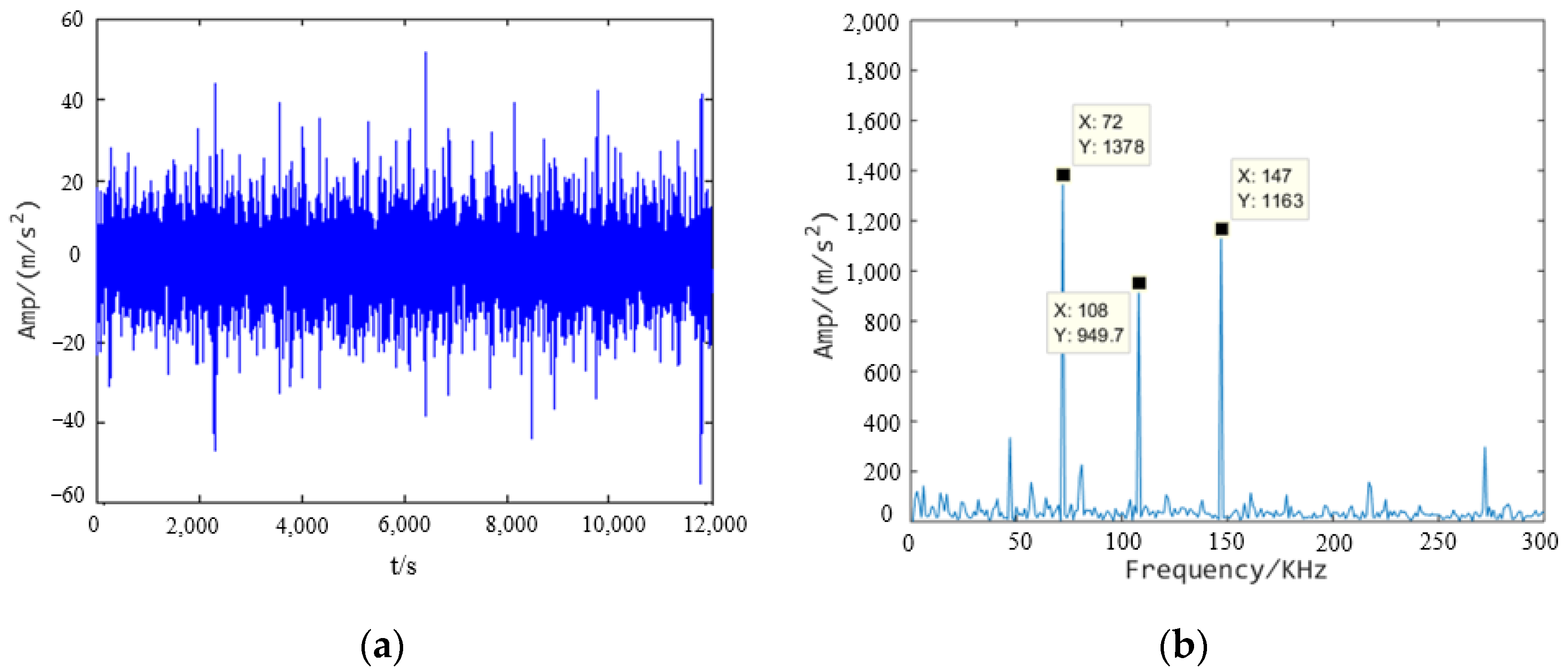
Figure 3 and
Figure 4.
From
Figure 2 to
Figure 4, it can be seen that the fault characteristic frequency of the shaft current damage is 72 Hz at 40 h, which is characterized by the fault characteristic frequency of the outer ring of the bearing, and the double frequency amplitude is also relatively large. At 60 h, the characteristic frequencies of 47 Hz, 72 Hz, and 108 Hz can be found in the spectrum diagram, which are the fault characteristic frequencies of the bearing balls, bearing outer rings, and bearing inner rings. In 80 h, the characteristic frequencies of 72 Hz, 147 Hz, and 108 Hz can be found in the spectrum, which are the double frequency, double frequency, and inner ring fault characteristic frequency of the outer ring fault. It can be concluded that in the shaft current damage experiment, 40 h is the initial wear stage of the bearing current damage. The initial wear pitting grooves have appeared on the bearing raceway and the ball surface, and the characteristic frequency of the outer ring fault has appeared. With the advancement of time, the bearing current damage has entered a sharp rise stage, and the fault characteristic frequency is manifested as a composite modulation form of multiple faults.
Although the bearing mechanical damage and bearing current damage bearing vibration signal characteristic frequencies in a certain correlation, because of the complexity of the bearing vibration signal of bearing current damage, only by the ordinary spectral analysis method is it difficult to effectively distinguish the bearing fault of bearing current damage and bearing mechanical damage.
5. Shaft Current Damage Identification Model of Motor Bearing Based on MFLP-MMT
Aiming at the characteristics of non-stationary, non-linear, and weak bearing fault signals, this paper proposes a fault diagnosis method combining multiscale sub-band fuzzy entropy and label propagation manifold distance metric. The multiscale sub-band fuzzy entropy can find the essential features of weak damage signals. At the same time, combined with the proposed label propagation manifold distance metric method, the distribution differences of the fault samples of motor bearings under different working conditions can be reduced, and bearing faults can be diagnosed and identified efficiently and accurately.
Based on the manifold distance metric of the graph label, the shaft current damage of motor bearing under variable working conditions is identified. Firstly, the GLP model is constructed using the samples with known fault types to obtain the pseudo labels of the unlabeled samples in the target condition. Locality preserving projection is performed on the source domain and the target domain samples and all samples are mapped to a low-dimensional manifold space. In the manifold space, by combining the labeled samples in the target domain obtained in GLP, the density ratio estimation is performed on the source domain samples to solve the sample weights, and the intra-domain metric learning is performed to obtain the optimal manifold distance metric in the manifold space. Under this metric, the samples in the source domain and the target domain can be transformed into the common subspace with the smallest cross-domain distance, the same sample clustering in the domain, and the alienation of different sample distributions, so that the differences of the sample distribution under variable working conditions can be eliminated. Finally, the fault samples are accurately classified according to the sample distribution in the manifold space.
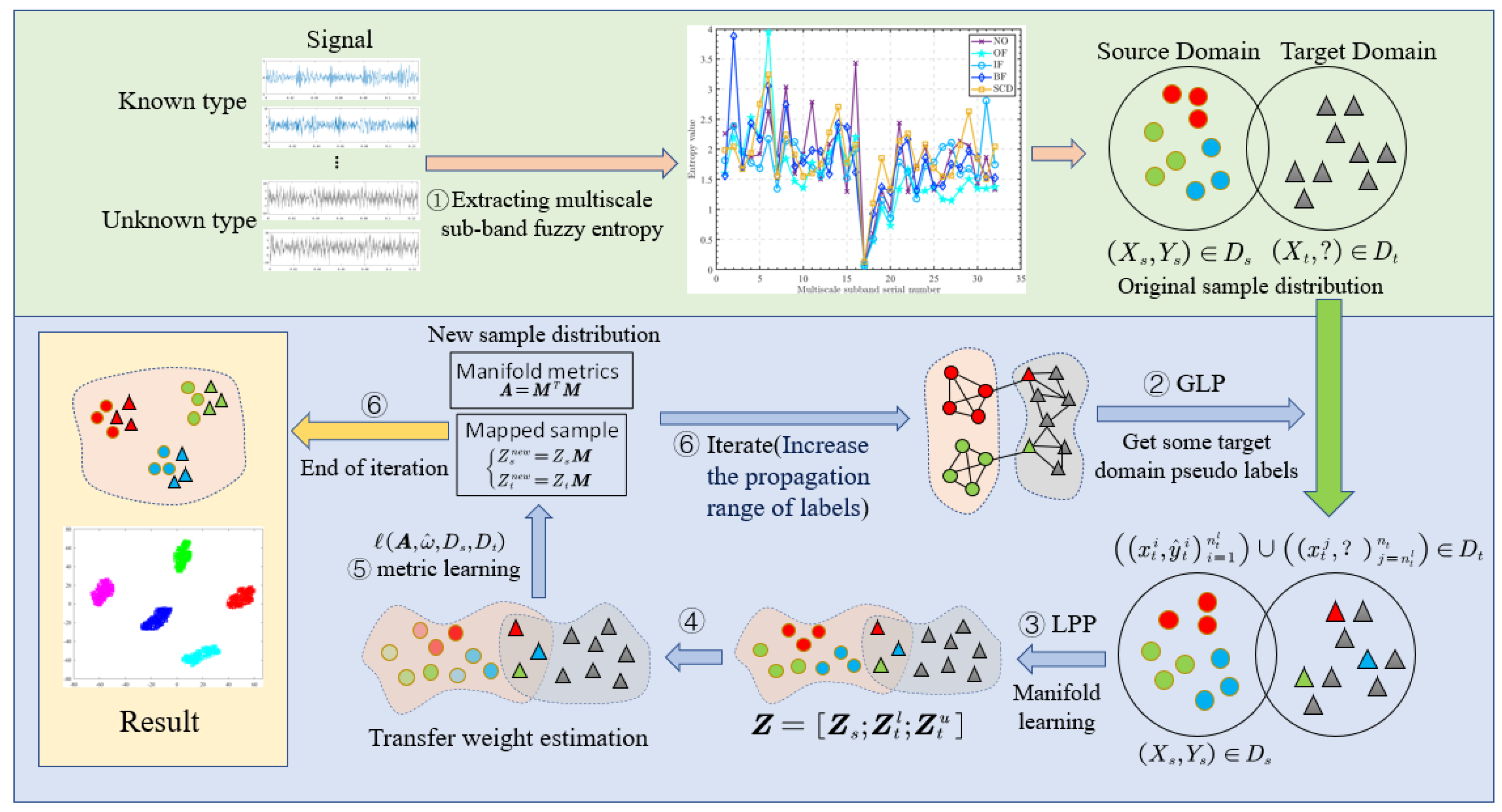
Since this shaft current damage identification method belongs to an unsupervised transfer learning, the fault samples to be identified in the target domain are unlabeled. In the process of learning, there is a certain error in the obtained target domain label. Therefore, we will gradually reduce the identification errors of the target domain samples by increasing the label propagation range in the iteration. The overall process of motor bearing shaft current damage identification proposed in this paper is shown in
Figure 5. The specific process can be divided into the following six steps:
Step 1: The bearing vibration signal with known label in one working condition is taken as the source domain and the signal data with an unknown label in another working condition is taken as the target domain . The vibration signal samples in the source domain and the target domain are extracted by multiscale sub-band fuzzy entropy as input.
Step 2: Based on GLP, transmits of the label information of the source domain samples to the target domain are used to obtain the pseudo label of the target domain. Based on the result of label propagation, a small part of the sample with the richest label information in the target domain is retained, that is, the sample closest to the source domain on the weighted graph. This part of the sample has a relatively small label error, and we retain this part of label information to obtain a new target domain with partial labels.
Step 3: According to the source domain sample and the target domain sample , the source domain and the target domain sample are projected locally, and the data in the original space is mapped to the D-dimensional manifold space to obtain .
Step 4: The cross-domain density ratio estimation of the source domain samples is calculated as a priori of the transfer weight . In order to obtain more reliable results, the samples with smaller label errors in the target domains are given 100% weight in the cross-domain transfer to obtain , and a more accurate sample weight in the source domain is obtained by regularization.
Step 5: Based on , a manifold metric is found, which can minimize the distribution difference between the source domain and the target domain in manifold space and eliminate the overlap between classes in the domain. Under this metric, the manifold regularization term is constructed and the manifold structure in the space is fully excavated, so that the cross-domain distance is smaller and the distinction between different classes is more obvious: and .
Step 6: The pseudo-label is updated according to the new sample distribution. After each iteration the label propagation range is increased and steps 2 to 6 are repeated until the results converge.
6. Experiments for Validation
6.1. Experiment on Shaft Current Damage Identification of Motor Bearing under Variable Working Conditions
In order to verify that the proposed method has better recognition ability for the typical faults of motor bearings under variable working conditions, the proposed method is compared with several popular transfer learning methods to evaluate the performance of the proposed method.
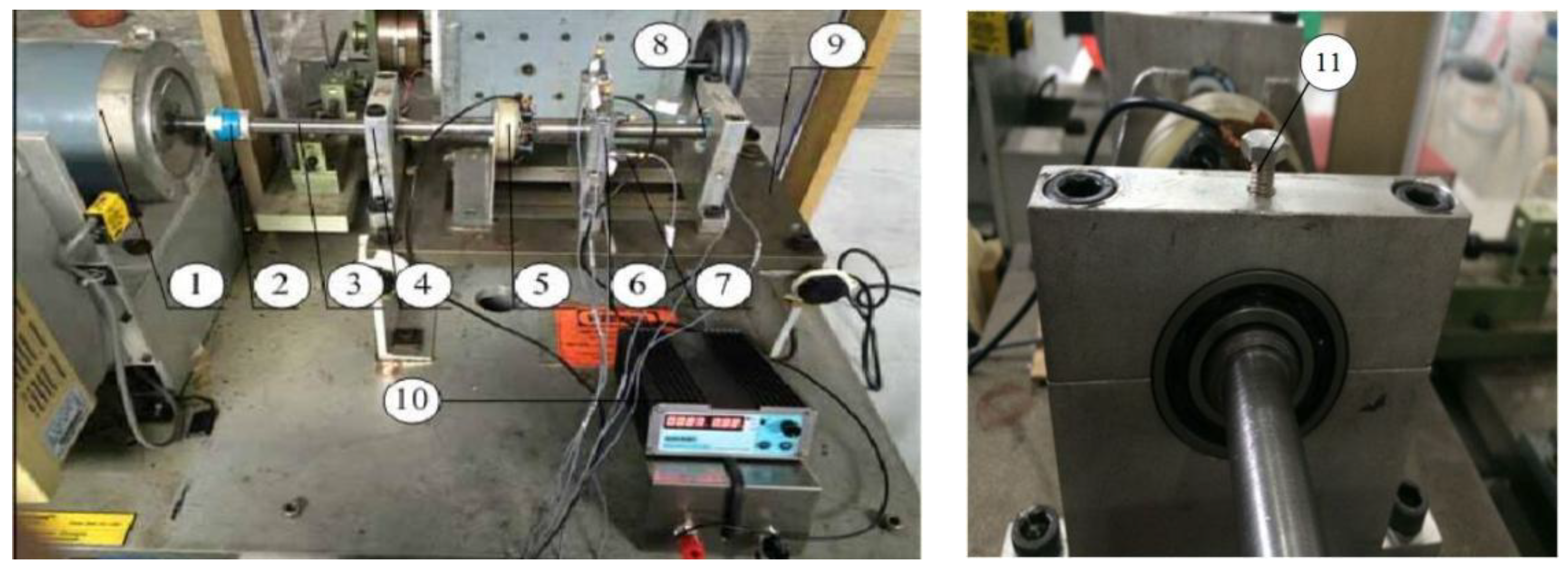
In this paper, the algorithm validation of a motor bearing shaft current damage simulation test bench is shown in
Figure 6. The test bearing used in this experiment is a detachable deep groove ball bearing whose model is 6205 EKA. Three different working conditions (500 N/1800 rpm, 1000 N/1200 rpm, 1500 N/600 rpm) were set in the experiment, and the sampling frequency was 16,384 Hz. The data used for verification have eight health states: normal (NO), outer ring fault (OF), inner ring fault (IF), rolling body fault (BF), and shaft current damage (SCD). There are 100 samples in each state of bearing, each sample contains 2048 data points, and each sample set has 500 samples in total. Three sample sets under different working conditions are obtained by labelling the data sets, and two data sets form a transfer task, so that six transfer tasks of damage identification under variable conditions can be obtained.
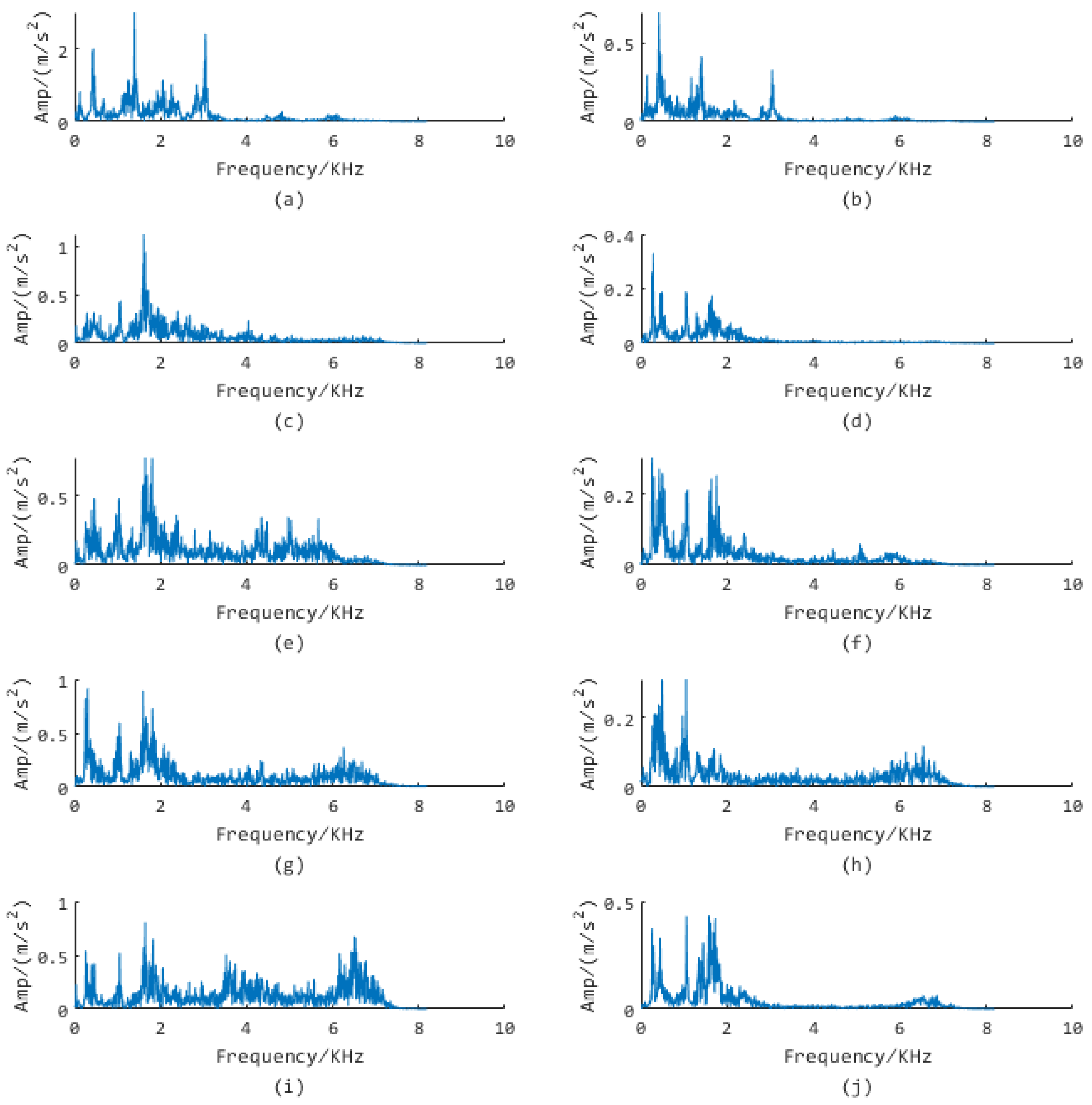
Furthermore, part of its signal spectrum is shown in
Figure 7. We can find that the spectrum of the same fault type varies greatly under different working conditions, especially the spectrum of shaft current damage, making it difficult to identify faults under variable working conditions.
6.2. Experimental Results
In order to reflect the effectiveness of the proposed method, we present the superiority of the proposed method from two aspects: One is to compare the multiscale sub-band fuzzy entropy with the ordinary time domain and frequency domain features (here we extract 24-dimensional time domain and frequency domain features, such as effective value, standard deviation, kurtosis, and average frequency). The second is to compare the proposed method with other machine learning algorithms and compare two typical traditional algorithms: KNN and SVM. There are two mainstream transfer learning methods, including one unsupervised transfer learning method, MEDA, and one semi-supervised metric transfer learning method, SSMTL [
47]. The transfer learning methods all use the KNN algorithm to obtain weak labels for the target domain. The initial subspace dimension is set to 10, and the same hyperparameters involved in the other algorithms are set to the same value. The regularization parameters in the algorithm are determined by optimizing from 0 to 1:
. The subspace dimension
, gradient descent step is set to a smaller value:
, gradient convergence threshold
, and iteration times
, The motor bearing fault identification results of five classification algorithms under different transfer tasks are obtained as shown in
Table 3, which is the result of all tasks.
Comparing different features, when the extracted features are the time domain and frequency domain features, the average recognition rate of the migration task of the proposed method is higher than that of other algorithms under variable working conditions. When the extracted features are multiscale sub-band fuzzy entropies, it can be seen that the accuracy of all methods is greatly improved compared with the ordinary time domain and frequency domain features. The MFLP-MMT method in this paper has the highest accuracy in all migration tasks, the average recognition rate is 99.97%, the standard deviation is the lowest, and the stability of the algorithm is the highest. It is proved that the proposed multiscale sub-band fuzzy entropy feature can deeply explore the essential characteristics of bearing vibration signals and can more clearly distinguish between the common bearing faults and current damage faults.
As one of the most basic classification methods, KNN does not change the original distribution of the classification samples and only measures the Euclidean distance between samples, so its average accuracy is always the lowest. As a widely used traditional classification method, the SVM method uses the inner product kernel function instead of the nonlinear mapping to the high-dimensional space, and the idea of maximizing the classification margin is the core of the SVM method. Therefore, SVM performs well in the sample classification of ordinary time-frequency domain features. However, when we extract multiscale features, the transfer learning method still has obvious advantages. As a metric transfer learning method, the SSMTL method measures and eliminates the distribution difference between the source domain and the target domain through the target domain supervision sample, so it can also have higher accuracy. The reason is that the different distributions of the variable condition samples are key problems that need to be solved by transfer learning.
Comparing the results of the transfer tasks A→C and C→A with those of the other tasks, it can be seen that the larger the span of the variable working conditions of the bearing, the worse the fault diagnosis effect. The reason is that the two sets of data with different working conditions have different spatial distributions, and the original space in which they are located covers its manifold characteristics. The larger the span of the working conditions, the greater the difference in the spatial distribution. In particular, for the transfer tasks A→C and C→A with a large span of variable working conditions, the recognition rate is also increased from about 80% to nearly 100%, which can better reflect the superiority of multiscale features. At the same time, the proposed MFLP-MMT method is used to fully mine the internal relationship of the data in the manifold space. Considering the inter-domain data offset, the source domain training samples are weighted. Further adjusting the distance between the classes in the domain can effectively avoid the overlap in the domain and adjust the spatial distribution of the data through iteration. The results show that the proposed method can effectively and accurately identify the multiple fault types of motor bearings under variable working conditions, and has a good performance, which is about 5% higher than the widely used unsupervised transfer learning method MEDA. The SSMTL method has high accuracy in tasks with a small migration span, but it is not effective when the working condition span is too large, so this is also its deficiency. As an unsupervised transfer learning algorithm, this method does not need to supervise the samples of the target working conditions, and all the damage identification tasks under variable working conditions are close to 100%, which reflects the superior performance of this method in the damage identification of bearing shaft current under variable working conditions.
6.3. Experimental Analysis
6.3.1. Comparison between Manifold Space and Linear European Space
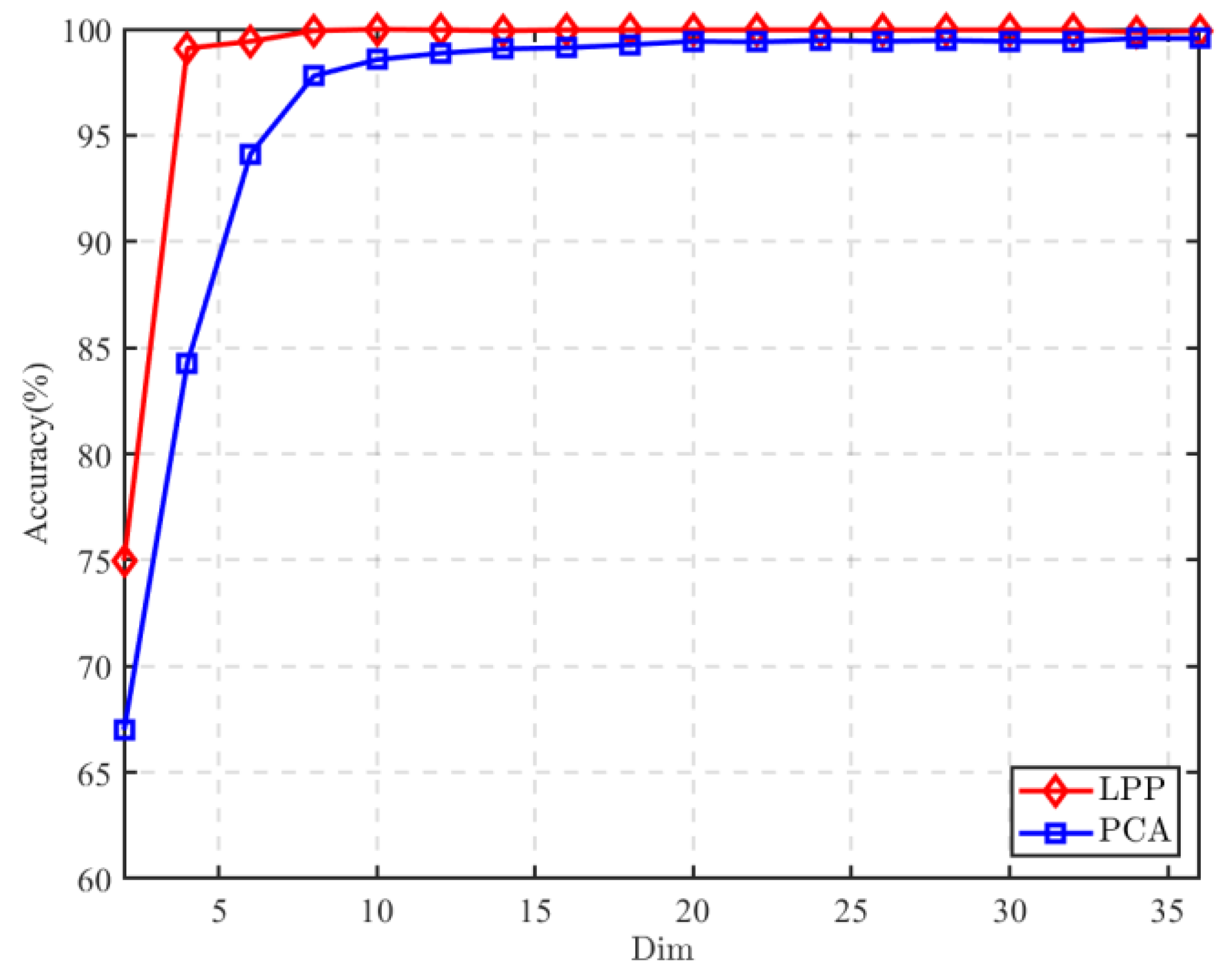
In order to reflect the importance of manifold mapping in this method, we compare the manifold mapping method LPP used in this method with the traditional linear dimensionality reduction method principal components analysis(PCA). By changing the dimension of the target projection space, the extracted multiscale sub-band fuzzy entropy features are implicitly projected into the target space to show the necessity of low-dimensional manifolds, and the experimental results are shown in
Figure 8.
From the figure, it can be seen that after the dimension reduction by LPP manifold, the fault recognition rate in all dimensions is higher than that of the traditional linear dimension reduction method PCA, and the advantage is more obvious when the spatial dimension is lower. In theory, the common fault of the same part of the motor bearing is very similar to the bearing current damage fault in the original space. As the spatial dimension changes, it can be found that the low-dimensional manifold space contains more sample information than the low-dimensional Euclidean space. As the spatial dimension changes, it can be found that the low-dimensional manifold space contains more sample information than the low-dimensional Euclidean space. When the manifold space dimension is about eight, the fault recognition accuracy is basically the highest. Using the linear dimension reduction PCA method, the fault recognition accuracy is positively correlated with the spatial dimension, indicating that the low-dimensional original space will lose sample information, indicating that the low-dimensional manifold mapping can indeed mine the hidden manifold structure in the original space. At the same time, the space with lower dimensions can reduce the complexity of the subsequent algorithm and reduce the computational cost.
6.3.2. Convergence Analysis of Algorithm
In order to study the convergence of the proposed method in the iterative process, we analyze the convergence of the algorithm for all variable working condition transfer tasks in the motor bearing fault data set and compare the two characteristics of the ordinary time domain frequency characteristics and multiscale sub-band fuzzy entropy. The results are shown in
Figure 9.
It can be seen from the figure that when the proposed features are the time domain and the frequency domain, some transfer tasks with small operating ranges can achieve more than 90% or even 100% accuracy through iteration. For the task A→C and task C→A with the large cross-domain transfer, because the ordinary time-domain and frequency-domain features cannot reflect the essential information of the vibration signal, when the operating conditions of the bearing are too different, the external information will be reflected. The characteristics of the vibration fault signal are then submerged, which makes the recognition rate of the fault classification method decrease significantly.
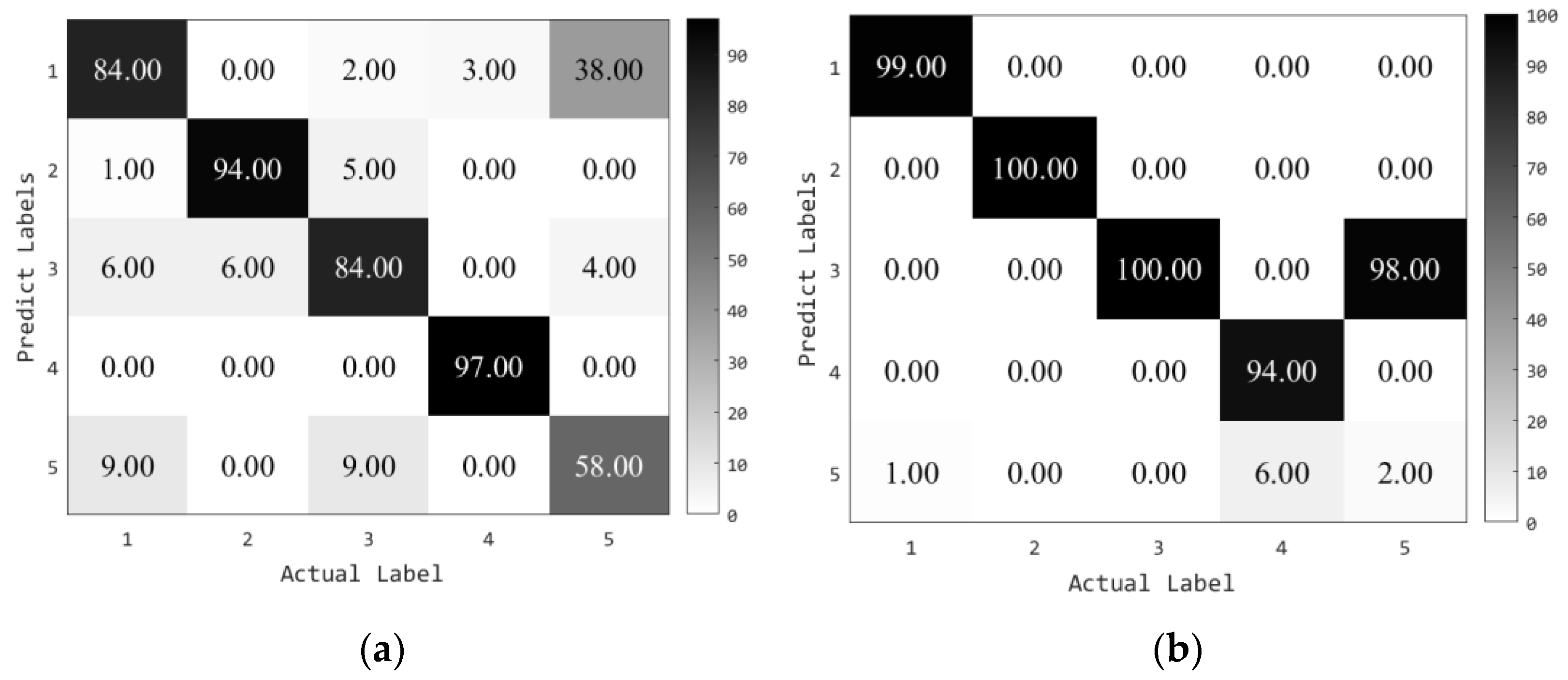
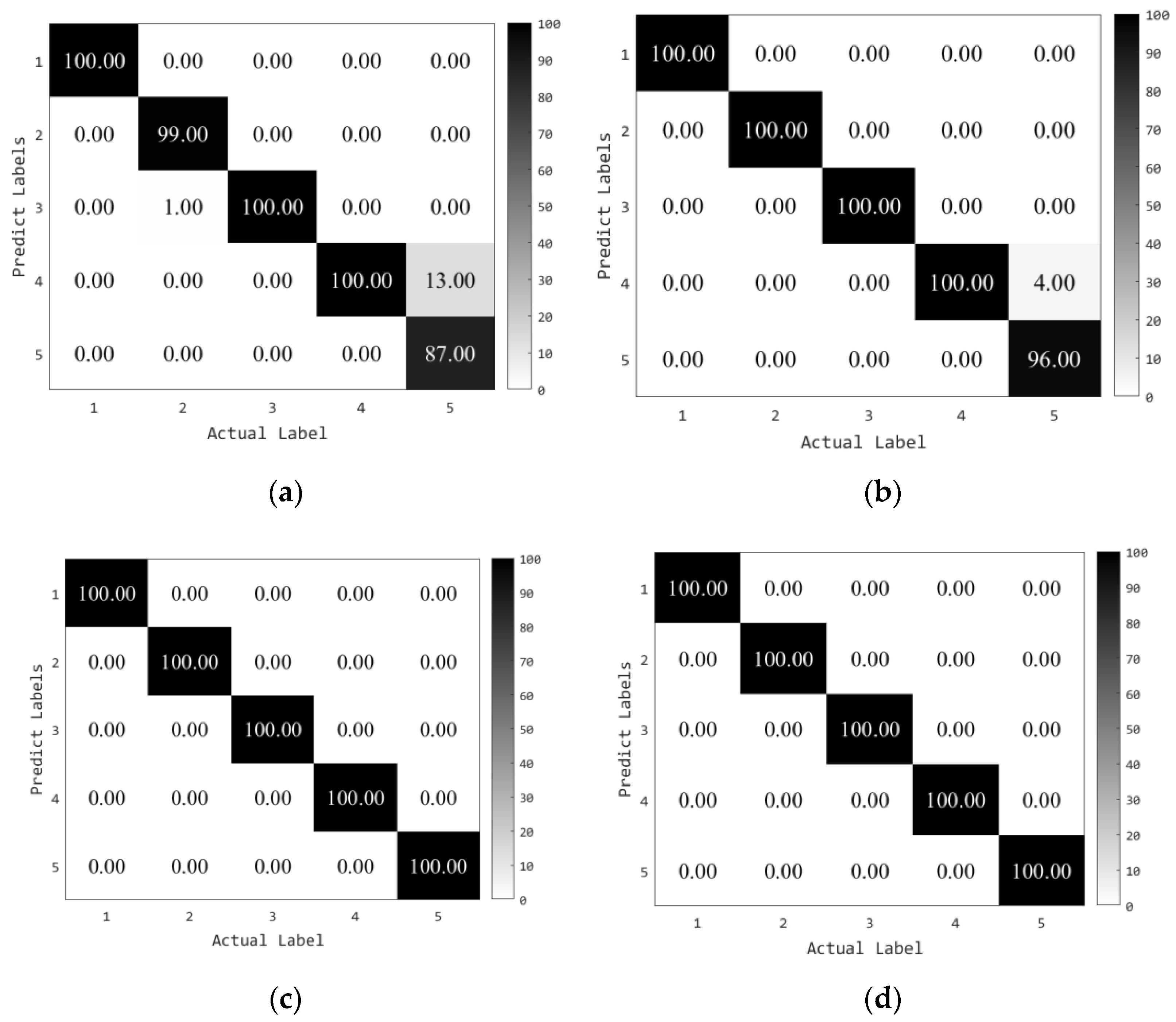
We analyze the recognition results of task A→C and task C→A through the confusion matrix. As shown in
Figure 10, we can see that the shaft current damage fault recognition rate of the motor bearing is the lowest in both transfer tasks. This is due to the damage process of the bearing current. It is a gradual evolution process. In the early stage of the damage, it is difficult to identify the shaft current damage fault of the bearing because the fault signal is too weak and the working condition changes too much. With the aggravation of the shaft current damage fault, the shaft current will form an electrical damage fault on the outer ring, ball, and inner ring of the motor bearing successively. Because the fault characteristics are not obvious, it is easy to confuse this kind of electrical damage fault with other common faults, which affects the maintenance and the repair of the equipment in the subsequent engineering practice.
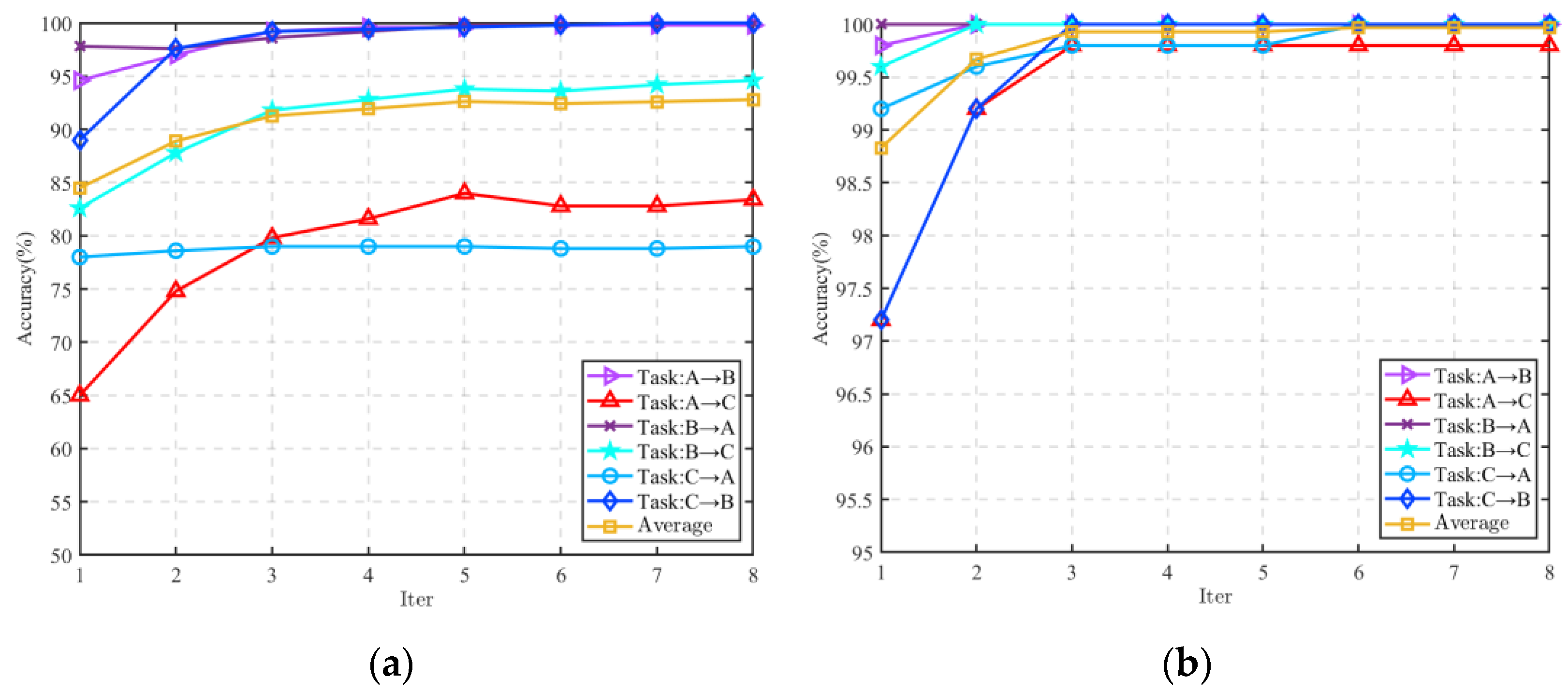
When the proposed feature is multiscale sub-band fuzzy entropy, the accuracy of the small part of the transfer task in the source domain and the target domain can reach more than 98% in the first iteration. Only one iteration can obtain a better recognition performance, and the recognition rate can be improved to about 100% after 2–3 iterations. Even if the sample label error after the first iteration is large, it can quickly converge to 100% during the iteration, as shown in
Figure 11 which is the transfer task C→B iterative convergence process. Furthermore, for all the transfer tasks in the iterative process, there is no significant decline in the identification accuracy, indicating that the proposed method has a good convergence.
6.3.3. Visual Analysis
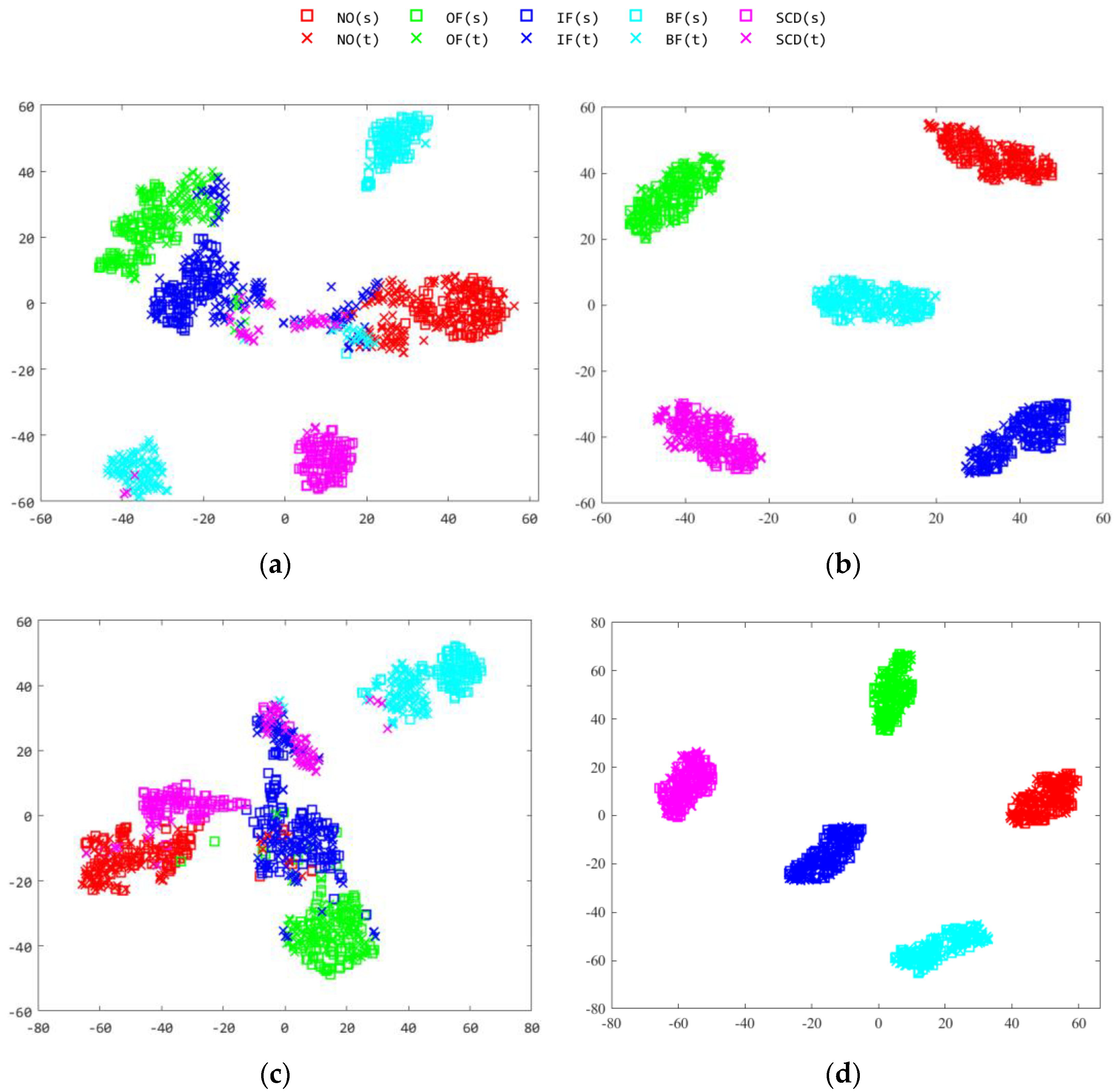
In order to observe the distribution of the data more intuitively, t-distribution stochastic neighbor embedding (t-SNE) algorithm is used to visualize the distribution of the fault types of tasks A→C and C→B and present the effect of the manifold measurement in the form of a two-dimensional scatter graph. As shown in
Figure 12, “□” represents the source domain sample and “×” represents the target domain sample.
It can be seen from the figure that, in the original space, the distribution of the fault type data under variable working conditions is quite different, and the overlap of the different types of motor bearing faults is serious. If the traditional machine learning algorithm is directly used for fault classification, it is easy to confuse the different fault types, especially for the motor bearing shaft. The recognition effect of the current damage is very poor. The proposed method can effectively reduce the cross-domain offset, while the same class of data narrows the distribution distance, achieving the effect of clustering and the distribution of different classes of samples of alienation, eliminating the overlap between classes within the domain, and achieving accurate identification of motor bearing shaft current damage.
7. Conclusions
In this paper, a method based on multiscale feature label propagation and manifold metric transfer is proposed to identify the shaft current damage of motor bearings under variable working conditions. By extracting multiscale sub-band fuzzy entropy, the essential characteristics of the weak damage signal of the motor bearings are deeply excavated. At the same time, it makes up for the shortcomings of the existing transfer learning methods in the fault diagnosis of bearing under variable working conditions, such as only the cross-domain distribution alignment, ignoring the distribution relationship between classes in the domain, and ignoring the label information in the domain. It solves the problems that the existing metric learning methods only focus on the metric of the original space and do not take into account the manifold relationship between the samples, and breaks the limitations of the need to supervise the samples in the process of the metric. By finding the manifold metric with the smallest cross-domain distance and obvious alienation of heterogeneous samples in the manifold space, the intra-domain overlap phenomenon of typical damage types of motor bearings is solved. Based on the graph label propagation method, the limited label information is gradually diffused in the manifold space to realize the cross-domain propagation of labels, and the problem of the low recognition accuracy of motor bearing shaft current damage under variable working conditions is solved. The experimental results show that the proposed method has a good recognition ability for typical faults of motor bearings and a strong convergence. The average accuracy of the diagnosis model is close to 100%. In industrial practice, different maintenance measures are taken, respectively, through the accurate diagnosis of the common faults and shaft current damage faults of the motor bearings. Moreover, the high accuracy of the fault diagnosis under variable working conditions greatly reduces the cost of the training diagnosis model. Only a labeled sample under one working condition can be collected, and the samples under other different working conditions can be efficiently identified.
In future work, we will continue to explore the recognition ability of MFLP-MMT in motor bearing current damage identification such as bearing current damage diagnosis for different types of motors.


