Article

Analysis, Modeling and Experimental Study of the Normal Contact Stiffness of Rough Surfaces in Grinding

State Key Laboratory of Tribology in Advanced Equipment, Tsinghua University, Beijing 100084, China
*
Author to whom correspondence should be addressed.
Lubricants 2023, 11(12), 508; https://doi.org/10.3390/lubricants11120508
Submission received: 25 September 2023 / Revised: 28 October 2023 / Accepted: 15 November 2023 / Published: 30 November 2023
(This article belongs to the Topic Advanced Manufacturing and Surface Technology)

Abstract

:
Grinding is the most important method in machining, which belongs to the category of precision machining processes. Many mechanical bonding surfaces are grinding surfaces. Therefore, the contact mechanism of grinding a joint surface is of great significance for predicting the loading process and dynamic characteristics of precision mechanical products. In this paper, based on the collected grinding surface roughness data, the profile parameters and topography characteristics of the asperity were analyzed, the rough surface data were fitted, the asperity profile was reconstructed, and the parabola y = nx2 + mx + l of the cylindrical asperity model was established. After analyzing the rough surface data of the grinding process, the asperity distribution height was fitted with a Gaussian distribution function, which proved that asperity follows the Gaussian distribution law. The validity of this model was confirmed by the non-dimensional processing of the assumed model and the fitting of six plasticity indices. When the pressure is the same, the normal stiffness increases with the decrease in the roughness value of the joint surface. The experimental stiffness values are basically consistent with the fitting stiffness values of the newly established model, which verifies the reliability and effectiveness of the new model established for the grinding surface. In this paper, a new model for grinding joint surface is established, and an experimental platform is set up to verify the validity of the model.

1. Introduction

The precision of grinding processing is high, and the combined surface of many parts is obtained by grinding. Therefore, it is of great theoretical significance to study the characteristics of grinding joint surfaces for the design of precision machinery. Normal contact stiffness is an important characteristic of grinding joint surfaces, which determines the running stability of mechanical parts. It is of practical value to study normal contact stiffness in order to improve the stability of mechanical equipment. In this paper, the asperity contact model is first established, then the contact stiffness formula is obtained, and the reliability of the model is verified by experiments. The establishment of an accurate and effective contact stiffness model for joint surfaces is the basis for further precision mechanical design, dynamic modeling, and analysis of machine tools. The modeling of a rough surface contact mechanism can be divided into a statistical model and a fractal model, according to the distribution of micro-convex bodies.
Greenwood and Williamson [1] were the first to study the rough surface contact problem with statistical methods, namely the GW model. Based on Hertz’s contact theory and combined with statistical principles, they systematically studied the contact mechanism of rough surfaces. In this model, the contact between the upper and lower rough bonded surfaces is equivalent to the contact between a spherical asperity and a smooth rigid plane. All the asperities are uniformly distributed on the matrix, and the asperities have the same curvature radius and are isotropic. Matrix deformation is ignored, only elastic deformation occurs in the slight asperity, and plastic deformation is ignored. The height of the asperities accords with Gaussian distribution, and the interaction between asperities is ignored. The asperities are assumed to be independent of each other. In view of the above limitations of the GW model, scholars have further improved on his research and put forward many revised models. Chang et al. [2] proposed a volume-invariant statistical model, namely the C.E.B. model, based on the volume conservation principle of asperities. The traditional model is compared with the numerical results of this model. The comparison results show that the previous analysis, which did not consider the volume conservation of asperities, is slightly improved. Kogut and Etsion [3] established an elastic–plastic finite element model (the KE model) considering the elastic–plastic deformation factors of asperities. The contact mechanism of rough surface asperity in the pure elastic, elastoplastic, and completely plastic deformation stages was analyzed. Wenzhen Xie et al. [4] studied the influence of roughness size on critical interference through an molecular dynamics (MD) simulation and proposed a critical interference fitting formula considering the effect of roughness size based on the results of an MD analysis and the traditional contact model. Hossein Jamshidi et al. [5] considered the influence of elastic substrate deformation on the friction coefficient, and established a statistical model of frictional contact between a hard rough surface and an elastic substrate by using the multi-rough surface contact theory. Hehe Kang et al. [6] proposed a statistical model to describe the normal and tangential contact behavior of multi-scale rough interfaces, considering the coupling effects of macro-profile deviation and mesoscopic roughness on contact behavior. Bo Yuan et al. [7] proposed an acoustic model combined with the microwave transmission line theory that considered contact interface and boundary effects. Li wei et al. [8] established the tangential contact model of the lap interface with a non-Gaussian surface.
Majumdar and Bhushan [9] used a fractal function (the WM function) to characterize the contours of a rough surface, and proposed, for the first time, a contact model based on fractal geometry theory, namely the MB model. When the power law spectrum of the surface profile falls within the fractal range, the multi-scale roughness structure can be characterized by fractal geometry. Xie yuanhong et al. [10] calculated the contact stiffness formula of a non-uniform interface of nodes with multi-rough surface contact characteristics at the microscopic level by using the fractal contact theory, and built a creep classification model of composite materials based on the elastic–viscoplastic theory. The elastic–viscoplastic contact mechanism of the fractal contact theory varying with time was further studied. Shen fei [11] used the three-dimensional Weierstrass–Mandelbrot (WM) function to characterize the fractal function parameters of rough surfaces. Yu xin et al. [12] equated the rough surface area to oil film thickness, derived the analytical formula for oil film thickness, and established a generalized closed fractal model of the friction coefficient between fractal surfaces in mixed lubrication. Chen hongxu et al. [13] analyzed the effects of fractal dimensions, fractal roughness parameters and Meyer index on contact stiffness, and constructed a modified fractal roughness model to calculate the contact stiffness of fixed joints. Chen Jian et al. [14] analyzed and studied the dynamic contact performance of engineering surfaces according to the scale dependence of key contact parameters of rough surfaces and the size distribution of contact points and proposed a fractal contact model considering multi-scale effects. Wang et al. [15] analyzed the loading and unloading process of a cylindrical friction surface and established a fractal contact model for a spherical micro-convex body. Yuan et al. [16] established an elastic–plastic contact model for the loading and unloading of three-dimensional rough fractal surfaces. Zhou et al. [17] used the maximum peak-to-peak ratio (VPR) to establish a three-dimensional convex and convex model of rough surfaces.
Most of the traditional models are based on the G.W. model, which is based on the spherical micro-convex hypothesis. In addition, there are elliptic micro-convex, two-dimensional asperity, normal curve asperity, residual curve asperity and other different shape asperity models. Fei shen et al. [18] proposed a multi-micro-convex type contact model based on the size distribution law of truncated region of rough surface. Qiuping Yu et al. [19] established the shoulder–shoulder contact geometric model of the rough sealing surface. Linbo zhu et al. [20] proposed a shoulder–shoulder contact normal contact stiffness model between rough body pairs considering three different contact modes of three-dimensional topography and rough surface elasticity, elastic–plastic and full-plastic. Wenzhen xie et al. [21] simulated the microscopic contact behavior of rough surfaces through molecular dynamics and established a semi-analytical model based on this. Lan zhang et al. [22], based on statistical methods, proposed a modified rectangular micro-convex model for the continuous observation of the length of non-adherent rough contact. Guangbin yu [23] comprehensively analyzed the geometric structure and mechanical properties of elliptical concave and convex points on rough surfaces, and established a contact mechanical model of elliptical asperities on rough surfaces containing elliptical concave and convex points. In order to accurately predict the leakage rate of the sealed interface, Bao lv et al. [24] established a two-dimensional finite element model of proton-exchange membrane fuel cells by analyzing the microscopic surface morphology and the rough contact process of components. Chaodong Zhang et al. [25] established a new contact stiffness model with sawtooth, normal function, and trapezoid contact stiffness of a textured rough surface by analysing the three kinds of machining surface textures: turning, milling and grinding. An qi et al. [26] adopted novel cosine curve roughness and traditional Gaussian distribution to simulate rough surfaces, and established a cosine curve asperity contact stiffness model. Li ling et al. [27] introduced the triangular distribution function and established the triangular distribution function contact stiffness model. Jiang kai et al. [28], considering the different surface contact characteristics of rough matrix interactions, used mesh regeneration technology to reconstruct the real surface topography, estimated the fractal parameters using the fractal parameters estimation neural network method, and established a mesh regeneration finite element model.
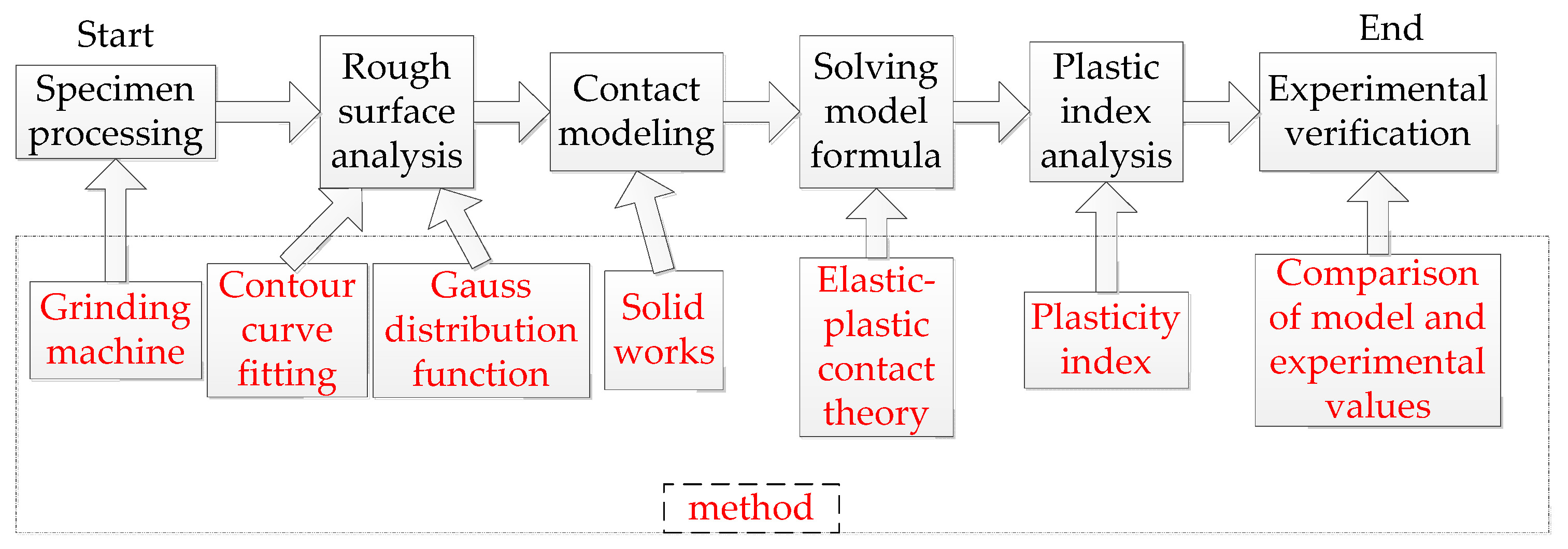
Based on the above review and an analysis of existing models, this paper collects the rough surface data of grinding processing, analyzes the profile parameters and topography characteristics of asperity, fits the rough surface data, resimulates the profile of asperity, and establishes a new parabola y = nx2 + mx + l cylindrical asperity model. An experimental platform is set up to verify the effectiveness of the new model. In Figure 1, for ease of understanding, the technical route flow chart is presented.

2. Hypothetical Surface

The study of the contact mechanism of rough bonded surfaces starts with a microscopic morphology of rough surfaces. The surface microstructure features were revealed, and the contact law was analyzed based on mechanical principles. In order to reveal the micro-morphology of the rough surface, a 3D white light interferometer was used to measure the grinding surface and obtain the precise data of the surface micro-morphology. By fitting the real topography data obtained from the measurement, the grinding simulation surface was established.
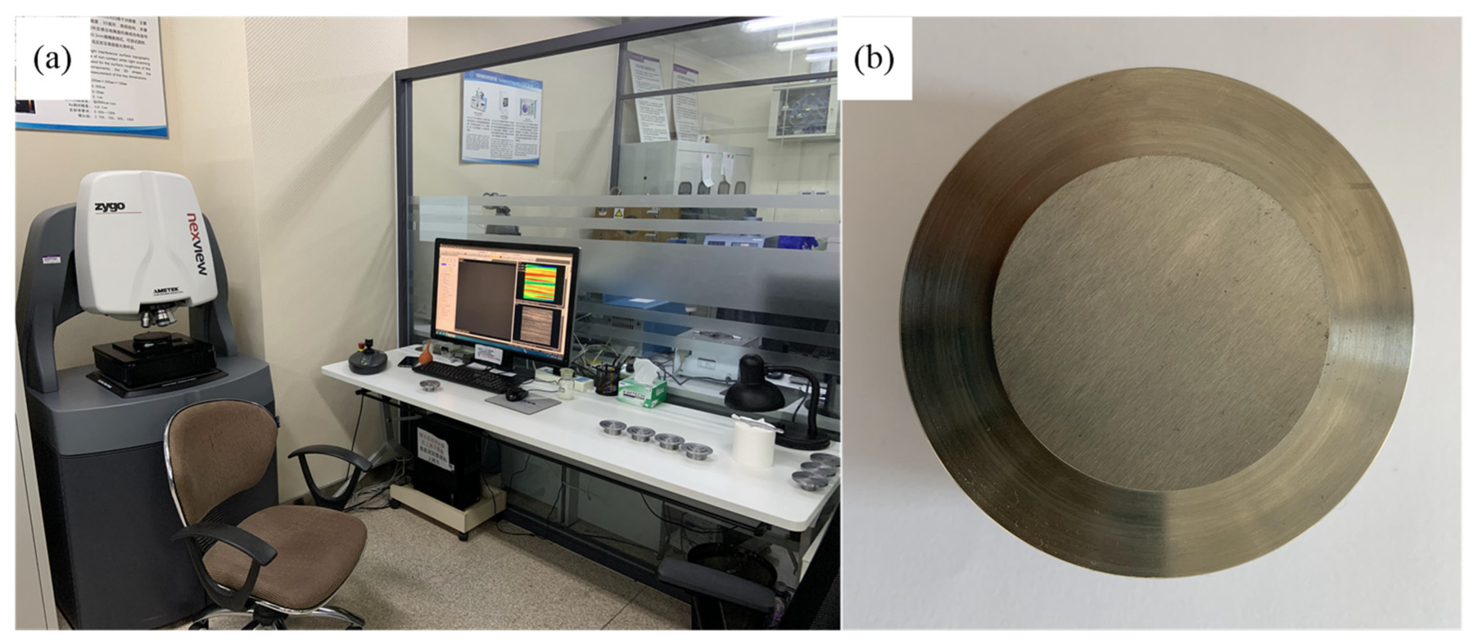
As shown in 
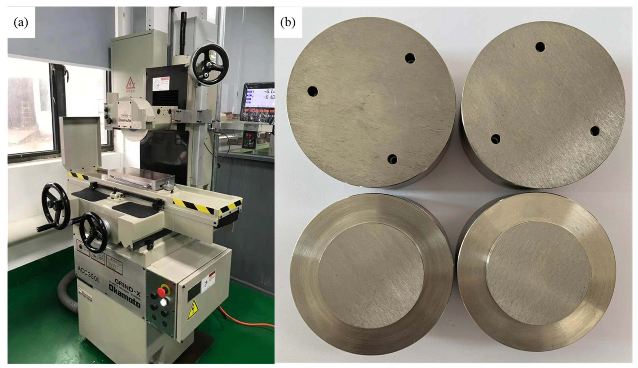
Figure 2a, ZYGONexView (ZYGO Connecticut, Middlefield, CT, USA), a practical 3D white light interferometer tested in this paper, is a high-linear-capacitance sensor. The accuracy of the instrument is to ensure the full range of 0.1 nm in 0–150 μm to ensure real and effective measurement results. Figure 2b shows the specimen obtained by grinding.
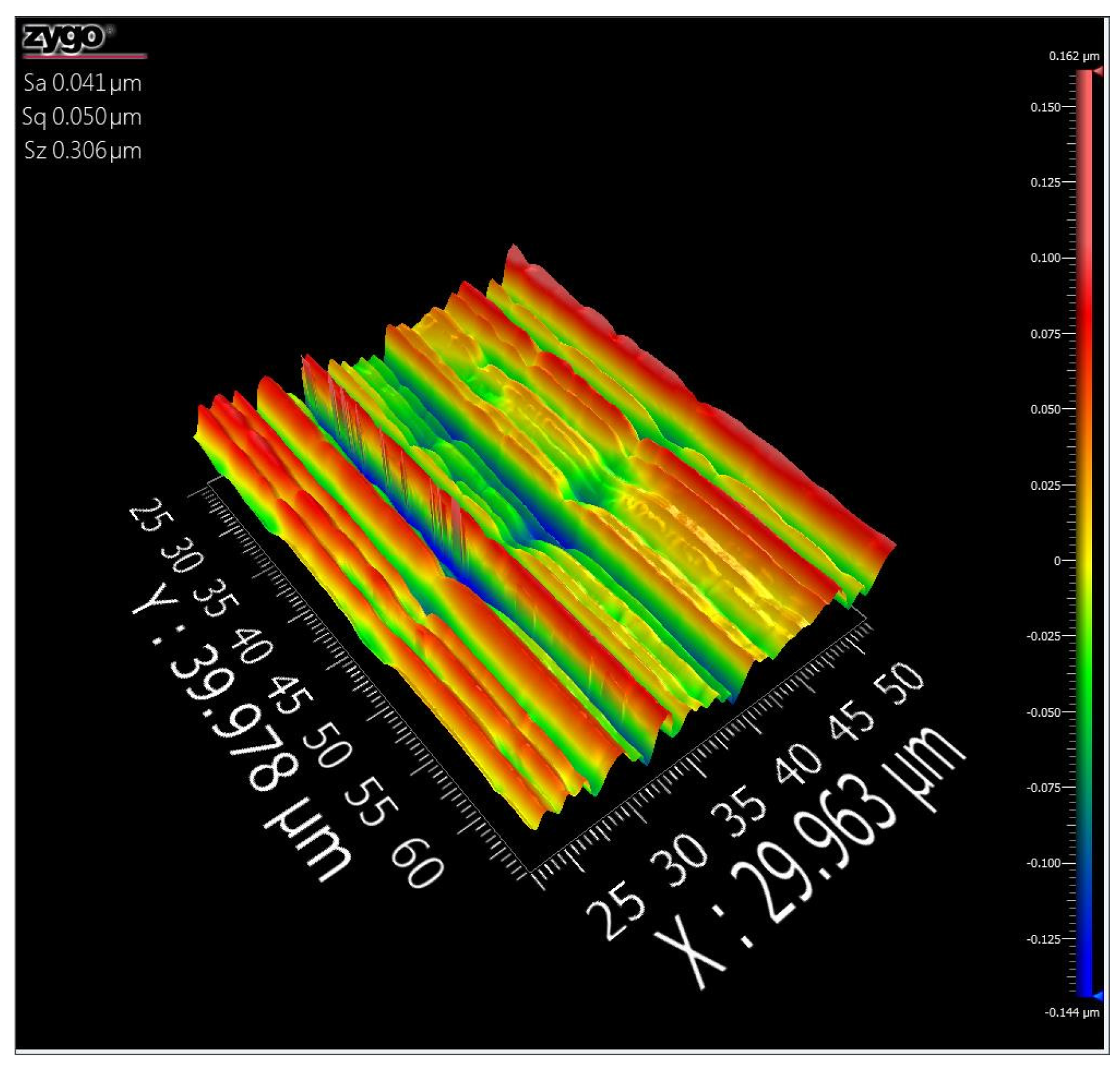
Figure 3 shows the 3D micromorphologies of grinding specimens obtained by 3D white light interferometer test. By observing their appearance, many strips of asperity are shown to be evenly and neatly distributed on the surface of the specimen, and the surface asperity is undulating, concave and convex, and the groove texture is clear.
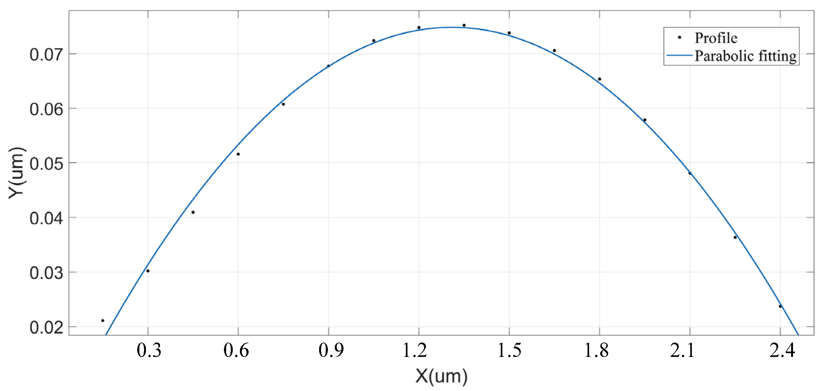
In order to reveal the real topography characteristics of the rough surface, the actual contour characteristics of a single asperity are tested. Then, the parabolic function y = nx2 + mx + l is used to fit the profile data points of the asperity cross-section. The fitting results are shown in Figure 4, and the fitting data points of the profile of the asperity cross-section are basically consistent with the curve of the parabola function. This proved that the distribution of data points of a single asperity cross-section on the rough surface obtained by grinding is close to the parabolic function curve.
In order to verify the superiority of the function y = nx2 + mx + l fitting, parabolic function y =cx3 and trigonometric function gsin (x) were used to fit the profile data points of the asperity cross-section. A root mean square error (RMSE) analysis was performed on the fitting results, and the analysis results are shown in Table 1. It can be seen from the table that the root mean square error of fitting function y = nx2 + mx + l is the lowest, which proves that fitting function y = nx2 + mx + l is the most suitable for fitting data points of the asperity cross-section.
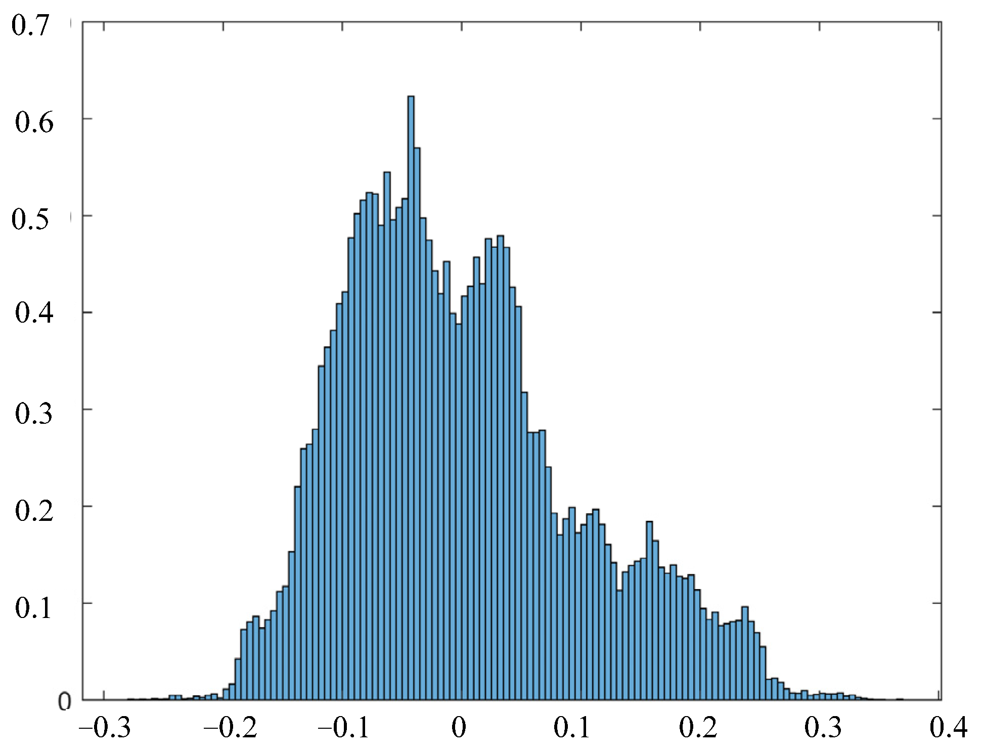
In order to obtain the height distribution of the rough surface, Gaussian distribution function is fitted to the data obtained by white light interferometer. The fitting results are shown in Figure 5, and the height distribution of the asperity on the rough surface conforms to the Gaussian distribution law.
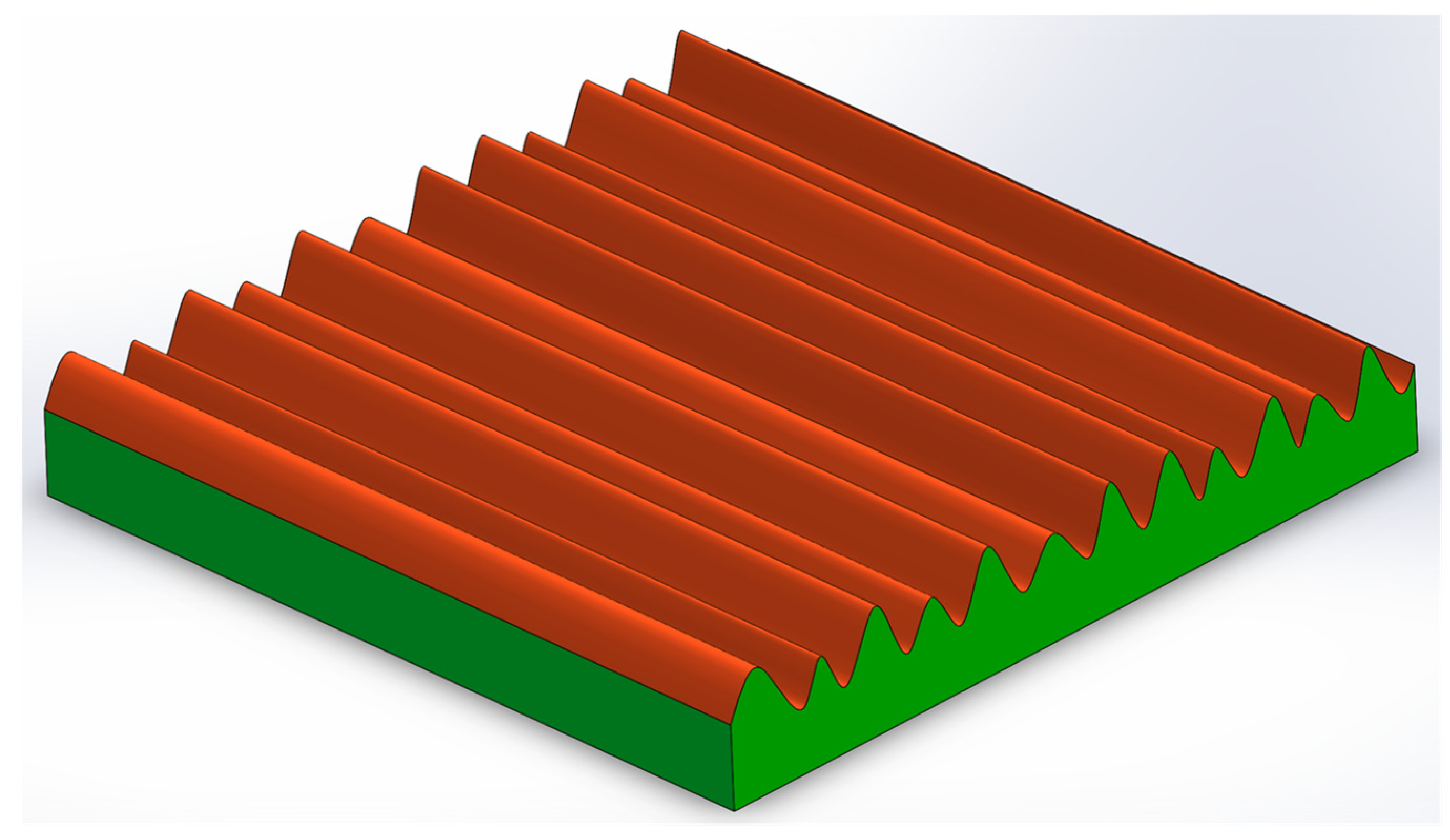
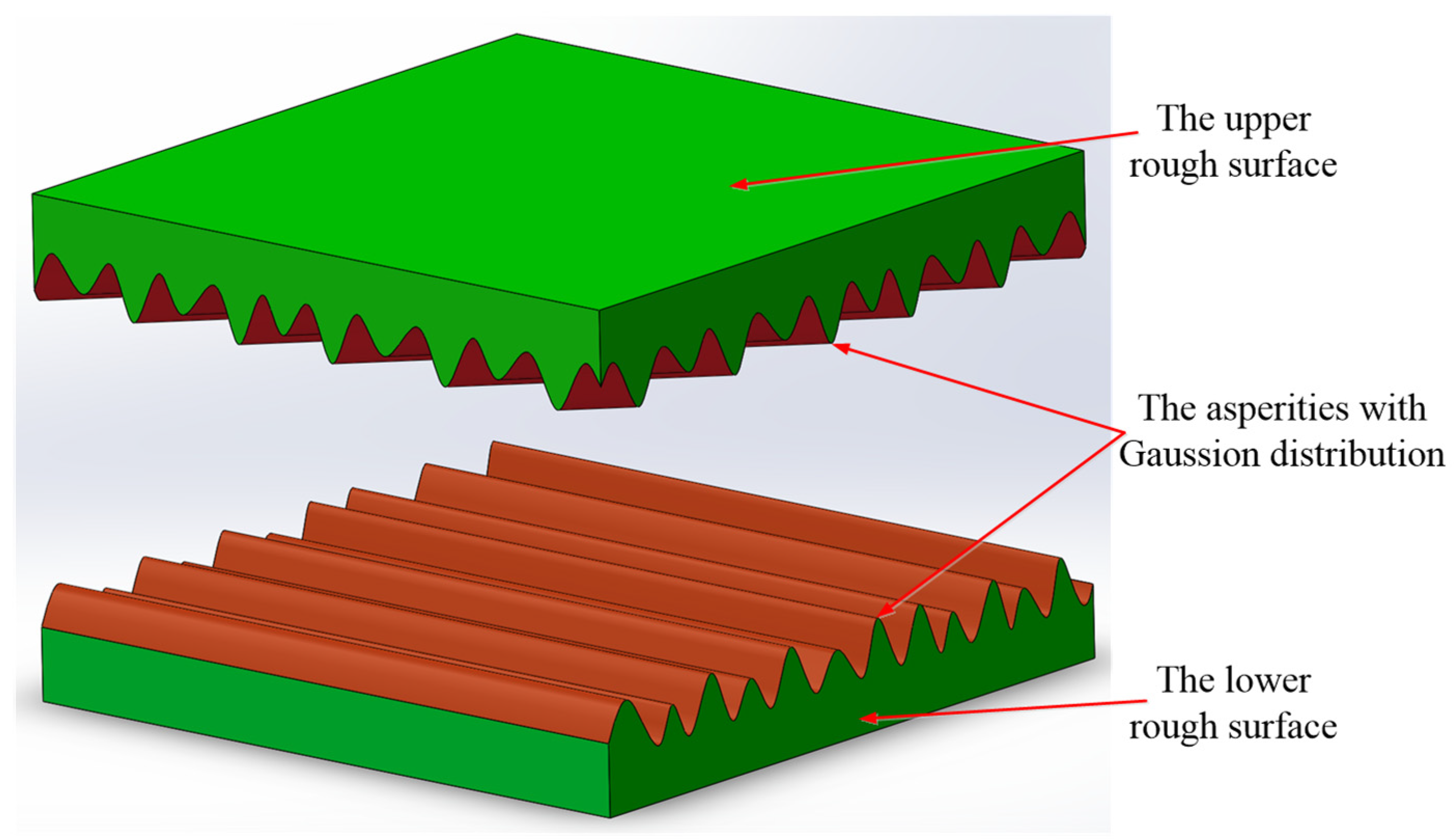
According to the above fitting analysis, the distribution of the data points of the cross-section of a single asperity on the rough surface is close to the curve of the parabolic function, and the height distribution of the asperity conforms to the Gaussian distribution law. Based on the above research results, this paper establishes a hypothetical surface with parabolic cylindrical asperity cross-section profile, and the height of asperity follows the Gaussian distribution law. As shown in Figure 6, it is assumed that the surface is more consistent with the real surface topography characteristics of grinding.

3. Normal Contact Stiffness Theoretical and Analytical Model

3.1. Contact Model Assumptions

In the previous section, a hypothesis surface with a parabolic cylindrical asperity cross-section profile was established by analyzing the micro-topography of the grinding surface. According to the surfaces assumed above, a theoretical analytical model of the normal contact stiffness of rough grinding surfaces is established in this section. The model made the following assumptions: (1) The contact of two rough surfaces is equivalent to the contact between two planes with evenly distributed asperity surfaces, and the cross-section outline of the asperity is a parabolic cylindrical asperity. (2) The angle between the cylindrical asperity of the upper and lower rough surfaces is 45° on average. (3) The height of the asperities follows the Gaussian distribution law. (4) The curvature radius of all asperity profiles is the same. (5) The asperities are independent of each other, ignoring the interaction between the asperities. (6) The texture direction of the asperity distribution on the rough surface is aligned. (7) Ignore the deformation of the matrix and only calculate the deformation of the asperity. Figure 7 shows the schematic diagram of the model hypothesis surface.
Based on the rough surface hypothesis model established above, the analytic formula of normal contact stiffness in the contact process of a single asperity is derived based on Hertzian contact theory. Then, according to the distribution law of the asperity and the statistical theory, the analytical formula of the contact stiffness of the whole joint surface is obtained.

3.2. Contact Stiffness of Mechanical Joint Surface

According to Reference [29], the stiffness of the whole rough surface of the asperity at different deformation stages is obtained below.
The relation between contact load and displacement variable is as follows:
F t ( d ) = F e t ( d ) + F e p t ( d ) + F p t ( d ) = N d d + ω 1 2 F e t Φ ( z ) d z + N d + ω 1 2 d + ω 2 2 F e p t Φ ( z ) d z + N d + ω 2 2 F P t Φ ( z ) d z = η A n E d d + ω 1 2 32 R ( z d ) 3 3 λ 3 2 1 2 π σ e - ( z d ) 2 2 σ 2 d z + 9 η A n R 2 ( π α β ) 3 16 E 2 d + ω 1 2 d + ω 2 2 ( H 0.6 H ln ω 2 ln 2 ( z d ) ln ω 2 ln ω 1 ) 3 [ 1 2 ( 2 z 2 d ω 1 ω 2 ω 1 ) 3 + 3 ( 2 z 2 d ω 1 ω 2 ω 1 ) 2 ] 3 1 2 π σ e - ( z d ) 2 2 σ 2 d z + 4 π η A n R H d + ω 2 2 ( z d ) 1 2 π σ e - ( z d ) 2 2 σ 2 d z
The relation between contact stiffness and displacement variable is as follows:
K t ( d ) = K e t ( d ) + K e p t ( d ) + K p t ( d ) = N d d + ω 1 2 K e t Φ ( z ) d z + N d + ω 1 2 d + ω 2 2 K e p t Φ ( z ) d z + N d + ω 2 2 K P t Φ ( z ) d z = η A n E d d + ω 1 2 8 R ( z d ) λ 3 2 1 2 π σ e - ( z d ) 2 2 σ 2 d z + 27 η A n ( π α β ) 3 R 2 16 E 2 d + ω 1 2 d + ω 2 2 { 0.6 H 2 ( z d ) ( ln ω 2 ln ω 1 ) [ H 0.6 H ln ω 2 ln 2 ( z d ) ln ω 2 ln ω 1 ] 2 [ 1 2 ( 2 z 2 d ω 1 ω 2 ω 1 ) 3 + 3 ( 2 z 2 d ω 1 ω 2 ω 1 ) 2 ] 3 + [ H 0.6 H ln ω 2 ln 2 ( z d ) ln ω 2 ln ω 1 ] 3 [ 1 2 ( 2 z 2 d ω 1 ω 2 ω 1 ) 3 + 3 ( 2 z 2 d ω 1 ω 2 ω 1 ) 2 ] 2 [ 6 ( 2 z 2 d ω 1 ) ( ω 2 ω 1 ) 2 6 ( 2 z 2 d ω 1 ) 2 ( ω 2 ω 1 ) 3 ] } 1 2 π σ e - ( z d ) 2 2 σ 2 d z + 2 π η A n R H d + ω 2 2 1 2 π σ e - ( z d ) 2 2 σ 2 d z

3.3. Dimensionless Processing of the Model

The characteristics of the contact stiffness model reveal the essential characteristics of the mechanical bonding surface, involving the displacement, loading size, loading time and other complex factors, involving more dimensions. Therefore, the features it embodies should avoid the influence of dimensions. For easier comparison between the models, it is necessary to carry out a dimensionless processing of the models.
Dimensionless load F* and dimensionless stiffness K* are obtained by dividing Equations (1) and (2) by AnE and (AnE)/σ, and all corresponding variables and length parameters in the formula are divided by σ for dimensionless processing.
F t ( d ) = F t ( d ) A n E = η h y h y + ω 1 2 32 R ( z h + y ) 3 3 λ 3 2 σ 2 π σ s e - σ 2 ( z h + y ) 2 2 σ s 2 d z + 9 η R 2 ( π α β ) 3 16 E 3 h y + ω 1 2 h y + ω 2 2 ( H 0.6 H ln ω 2 ln 2 ( z h + y ) ln ω 2 ln ω 1 ) 3 [ 1 2 ( 2 ( z h + y ) ω 1 ω 2 ω 1 ) 3 + 3 ( 2 ( z h + y ) ω 1 ω 2 ω 1 ) 2 ] 3 σ 2 π σ s e - σ 2 ( z h + y ) 2 2 σ s 2 d z + 4 π η R H E h y + ω 2 2 ( z h + y ) σ 2 π σ s e - σ 2 ( z h + y ) 2 2 σ s 2 d z
By substituting β = ηRσ into the formula:
F t ( d ) = F t ( d ) A n E = β ( σ R ) 1 2 h y h y + ω 1 2 32 ( z h + y ) 3 3 λ 3 2 σ 2 π σ s e - σ 2 ( z h + y ) 2 2 σ s 2 d z + β R σ 9 ( π α β ) 3 16 E 3 h y + ω 1 2 h y + ω 2 2 ( H 0.6 H ln ω 2 ln 2 ( z h + y ) ln ω 2 ln ω 1 ) 3 [ 1 2 ( 2 ( z h + y ) ω 1 ω 2 ω 1 ) 3 + 3 ( 2 ( z h + y ) ω 1 ω 2 ω 1 ) 2 ] 3 σ 2 π σ s e - σ 2 ( z h + y ) 2 2 σ s 2 d z + 4 β π H E h y + ω 2 2 ( z h + y ) σ 2 π σ s e - σ 2 ( z h + y ) 2 2 σ s 2 d z
F t ( d ) = K t ( d ) σ A n E = η σ h y h y + ω 1 2 8 R ( z h + y ) λ 3 2 σ 2 π σ s e - σ 2 ( z h + y ) 2 2 σ s 2 d z + 27 η σ ( π α β ) 3 R 2 16 E 3 h y + ω 1 2 h y + ω 2 2 { 0.6 H 2 ( z h + y ) ( ln ω 2 ln ω 1 ) [ H 0.6 H ln ω 2 ln 2 ( z h + y ) ln ω 2 ln ω 1 ] 2 [ 1 2 ( 2 ( z h + y ) ω 1 ω 2 ω 1 ) 3 + 3 ( 2 ( z h + y ) ω 1 ω 2 ω 1 ) 2 ] 3 + [ H 0.6 H ln ω 2 ln 2 ( z h + y ) ln ω 2 ln ω 1 ] 3 [ 1 2 ( 2 ( z h + y ) ω 1 ω 2 ω 1 ) 3 + 3 ( 2 ( z h + y ) ω 1 ω 2 ω 1 ) 2 ] 2 [ 6 ( 2 ( z h + y ) ω 1 ) ( ω 2 ω 1 ) 2 6 ( 2 ( z h + y ) ω 1 ) 2 ( ω 2 ω 1 ) 3 ] } σ 2 π σ s e - σ 2 ( z h + y ) 2 2 σ s 2 d z + 2 π η σ R H E h y + ω 2 2 σ 2 π σ s e - σ 2 ( z h + y ) 2 2 σ s 2 d z
By substituting β = ηRσ into the formula:
F t ( d ) = K t ( d ) σ A n E = β ( σ R ) 1 2 h y h y + ω 1 2 8 ( z h + y ) λ 3 2 σ 2 π σ s e - σ 2 ( z h + y ) 2 2 σ s 2 d z + β R σ 27 ( π α β ) 3 16 E 3 h y + ω 1 2 h y + ω 2 2 { 0.6 H 2 ( z h + y ) ( ln ω 2 ln ω 1 ) [ H 0.6 H ln ω 2 ln 2 ( z h + y ) ln ω 2 ln ω 1 ] 2 [ 1 2 ( 2 ( z h + y ) ω 1 ω 2 ω 1 ) 3 + 3 ( 2 ( z h + y ) ω 1 ω 2 ω 1 ) 2 ] 3 + [ H 0.6 H ln ω 2 ln 2 ( z h + y ) ln ω 2 ln ω 1 ] 3 [ 1 2 ( 2 ( z h + y ) ω 1 ω 2 ω 1 ) 3 + 3 ( 2 ( z h + y ) ω 1 ω 2 ω 1 ) 2 ] 2 [ 6 ( 2 ( z h + y ) ω 1 ) ( ω 2 ω 1 ) 2 6 ( 2 ( z h + y ) ω 1 ) 2 ( ω 2 ω 1 ) 3 ] } σ 2 π σ s e - σ 2 ( z h + y ) 2 2 σ s 2 d z + 2 π β H E h y + ω 2 2 σ 2 π σ s e - σ 2 ( z h + y ) 2 2 σ s 2 d z
In the formula:
ω 1 = ω 1 / σ = 1.709 [ 9 128 R F 1 2 ( 1 - ν 1 2 E 1 + 1 - ν 2 2 E 2 ) 2 ] 1 3 = 0.000332811 R σ
ω* = ω/σ is the normal deformation of a single asperity after non-dimensionalization. ω1* = ω1 is the normal critical deformation of the asperity after dimensionless transition from the stage of complete elastic deformation to the stage of elastoplastic deformation. ω2* = ω2 is the normal critical deformation of the asperity from the elastoplastic deformation stage to the complete plastic deformation stage after dimensionless deformation. z* = z/σ is the height of a single asperity without dimensionalization; y* = y/σ is the distance between the mean height plane of the asperity and the mean height plane of the surface after non-dimensionalization. h* = h/σ is the distance between the average height planes of the upper and lower bound surfaces after being dimensionless.

3.4. Plasticity Index

The plasticity index, which is considered to be the standard of elasticity or plasticity of a rough surface, is essentially the ratio of elastic hardness to actual hardness. It can be seen from the plastic index that the contact of rough surface is determined by two material properties of plane stress elastic modulus and hardness, and three shape properties of rough surface asperity density, standard deviation of height distribution, and average radius. The plasticity index is a generalized surface morphology parameter that combines the material and morphology characteristics. For most rough surfaces, the deformation mode is not affected by the change of load, and the low plasticity index is elastic, with high plasticity index is plastic. According to the literature [2], the calculation formula of plasticity index can be obtained as follows::
ψ = 2 E 1.5 π K H ( σ R ) 1 2 ( 1 3.717 × 10 4 β 2 ) 1 4
It can be seen from the plasticity index formula that the contact characteristics of rough surfaces are determined by the values of β and σ/R. The plasticity index parameters were obtained by testing typical engineering rough surfaces and referring to the experimental data of K. A. NURI and J. HALLING [30], as shown in Table 2.

3.5. Dimensionless Stiffness Is Fitted by Simulation

Figure 8 shows the numerical simulation curves of the dimensionless contact stiffness and dimensionless contact pressure of the assumed rough surface, with plasticity indices of 0.5, 0.7, 1.0, 1.5, 2.0 and 2.5, respectively. The material is 304 steel; elastic modulus is E = 195 GPa; hardness H = 1870 MPa. Figure 8 shows the influence of different plasticity indices on normal contact stiffness. It can be seen from the figure that the contact stiffness increases with the increase in contact pressure. When the contact pressure is the same, the normal contact stiffness increases with the increase in plastic index. This is because the physical meaning of the plasticity index is to determine the elastic–plastic contact characteristics between two surfaces. When the contact load increases, the contact stiffness increases, and the increase in the contact stiffness of the surface with a high plasticity index is higher than that of the surface with a low plasticity index, which verifies the validity of this model.

4. Experiment

4.1. Experimental Specimen

The rough surface of the specimen in this experiment was obtained by grinding, and the material was 304 steel. The parameters of No. 304 steel are obtained by mechanical experiments: Young’s modulus E1 = E2 = 195 GPa; Poisson’s ratio ν1 = ν2 = 0.29; hardness H = 1870 MPa. Figure 9a shows the processing and molding equipment of this experiment specimen. The model is an okamoto ultra-precision static press surface grinding machine (Okamoto, Tokyo, Honshu, Japan), upg series. Figure 9b shows the normal contact stiffness test specimen. The bonding surface is the convex surface obtained by grinding, and the height of the convex surface is 2 mm. The roughness of the joint surface was Sa 0.854 μm, Sa 1.173 μm, Sa 1.391 μm and Sa 1.524 μm, respectively.

4.2. Experimental Apparatus

As shown in Figure 10, in order to verify the accuracy of the model presented in this paper, a normal contact stiffness test platform was built. Figure 10a shows the execution devices of the test platform, including four parts: pressure testing machine, compression module, data acquisition module and control module. The pressure testing machine is a W.D.W. series microcomputer controlled electronic universal testing machine (5–20 KN); the equipment test error is less than ±0.5%. Figure 10b shows the compression module, which consists of seven parts: compression rod, upper specimen, eddy current displacement sensor, lower specimen, link disk, thrust roller bearing and fixed column. The eddy current sensor is a KAMAN(KAMAN Bloomfield, CT, USA) high-precision eddy current displacement sensor, model KD2306-2U. The measuring accuracy is ±0.1 μm, the measuring range is 0–1 mm, and the output voltage is 0–10 V. The data acquisition module uses an Altai data collector, model PCIe5653.
Figure 10c reveals the working principle of the contact stiffness test platform of the grinding joint surface. The compression rod is connected to the pressure sensing part of the pressure testing machine, and the lower end of the compression rod is connected to the upper specimen. Three eddy current displacement sensors are installed in three holes, uniformly distributed along the edge of the upper specimen. The lower specimen is connected with a connecting disc, and a thrust roller bearing is installed between the connecting disc and the fixed column. The thrust roller bearing can effectively adjust the contact between the upper and lower two specimens, offset the installation error and ensure complete normal contact between the upper and lower two specimens, so that the pressure is evenly distributed throughout the joint surface. At the beginning of the test, the universal testing machine applies a normal load on the upper specimen through the compression rod so that pressure is generated between the upper and lower specimens. At this time, the joint surface is subjected to normal static force, and relative normal displacement will be generated. The eddy current displacement sensor converts the displacement into voltage and transmits it to the data acquisition module for storage. Combined with the loading data of the universal testing machine, the static compression force and relative deformation data of the joint surface are finally collected. In order to ensure the measurement accuracy, the average displacement value of three eddy current displacement sensors is taken as the test data.

5. Results and Discussion

In order to verify the reliability of the proposed model, the simulation stiffness of the proposed model is compared with the experimental stiffness. Roughness is an important parameter that determines the precision of the machined rough surface. The roughness values of four rough surfaces, Sa 0.854 μm, Sa 1.173 μm, Sa 1.391 μm and Sa 1.524 μm, were obtained by grinding in this experiment to verify the validity of the model. 
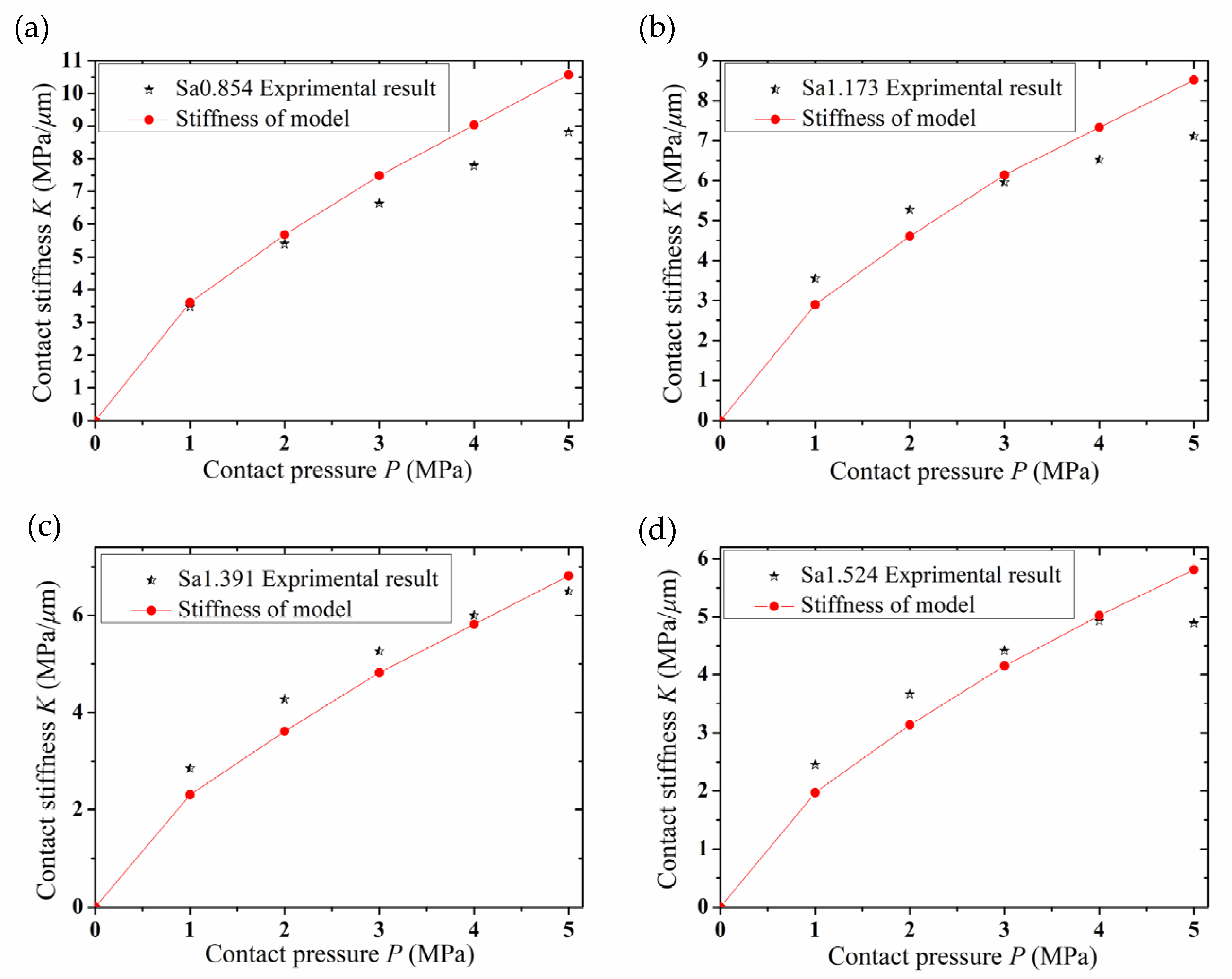
Figure 11 shows the comparison result curve between model simulation stiffness and experimental stiffness.
It can be seen from the figure that the experimental value of normal stiffness increases with the increase in normal pressure. When the normal pressure is the same, the normal stiffness increases with the decrease in roughness value. The roughness is Sa 0.854 μm, Sa 1.173 μm, Sa 1.391 μm and Sa 1.524 μm at different scales. When the normal contact pressure reaches 5 MPa, the simulated normal contact stiffness of the model reached 10.57 MPa/μm, 8.519 MPa/μm, 6.81 MPa/μm and 5.814 MPa/μm, respectively. When the asperity is subjected to normal load, the force on the top of the asperity is small, and the deformation is within the pure elastic range. In this case, the deformation of the asperity can be regarded as pure elastic deformation, and the relationship between normal load and stiffness can be regarded as linear. When the pressure increases, the deformation of the asperity gradually enters the elastoplastic deformation stage, the deformation of the asperity will be mainly elastoplastic, and the normal stiffness will gradually increase. When the normal contact load increases to a certain extent, most of the asperity deformation enters the plastic deformation stage, and the contact deformation of asperity is mainly plastic. With the increase in load, the deformation of the asperity finally enters the stage of complete plastic deformation. Therefore, the normal stiffness gradually increases with the increase in normal pressure. From the perspective of surface topography, when the pressure is the same, the density of asperity on the surface with high roughness is lower than that on the surface with small roughness, so the amount of asperity involved in the contact is relatively small, and the relative displacement is larger than that on the surface with small roughness, making the contact stiffness lower than that on the surface with small roughness. Through the above research, it is confirmed that the grinding surface topography affects the contact stiffness between mechanical parts, and the roughness affects the running state between components. By improving the grinding precision and reducing the roughness of the joint surface, the stability of mechanical equipment can be effectively improved.
It can be seen from the figure that the experimental stiffness curve value and the model stiffness curve value are basically consistent under four different roughness conditions, which proves that the model has certain application value. Firstly, by analyzing the micro-morphology of the grinding surface, this paper refits the profile curve of the asperity and establishes a parabolic cylindrical asperity hypothesis, which is more suitable for the grinding surface. The hypothesis of the model is more suitable for the actual contact state, which is conducive to improving the accuracy of the simulation stiffness value of the model. Secondly, according to the elastic–plastic theory, the contact deformation of the asperity is divided into three different stages, namely, elastic, elastic–plastic and complete plastic deformation stages, which reduces the fitting error of the model. Finally, this is used for the precision design of the measuring device in this experiment, and the testing mechanism is more reasonable and effective. In this experiment, a high-precision measuring instrument was used to improve the measuring accuracy.
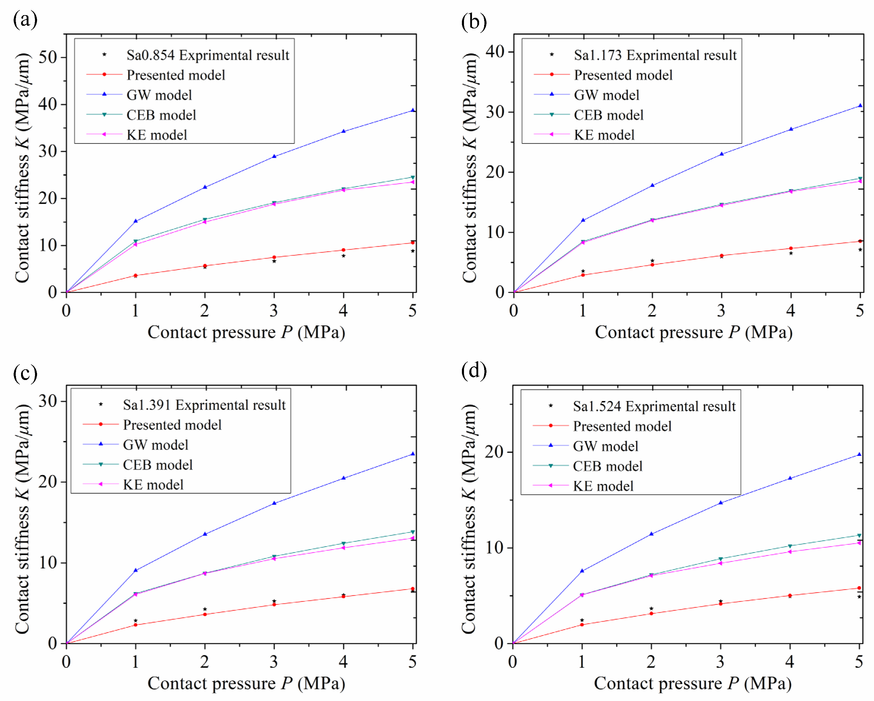
In order to verify the accuracy of the new model, the stiffness values of the present model, GW model, CEB model and KE model were compared with those of the experimental test. Figure 12 shows the comparison between the experimental contact stiffness values of Sa 0.854 μm, Sa 1.173 μm, Sa 1.391 μm and Sa 1.524 μm of test samples with different roughness values and the simulated stiffness values of each model.
As can be seen from Figure 12, the normal contact stiffness value keeps increasing with the increase in normal contact pressure. When the normal pressure reaches 5 MPa, the stiffness error of GW model is the largest, and the stiffness error of CEB model and KE model is relatively low compared with the GW model. The trend of the new model curve is basically the same as that of the experimental curve, and the simulated and experimental stiffness values are close to each other.
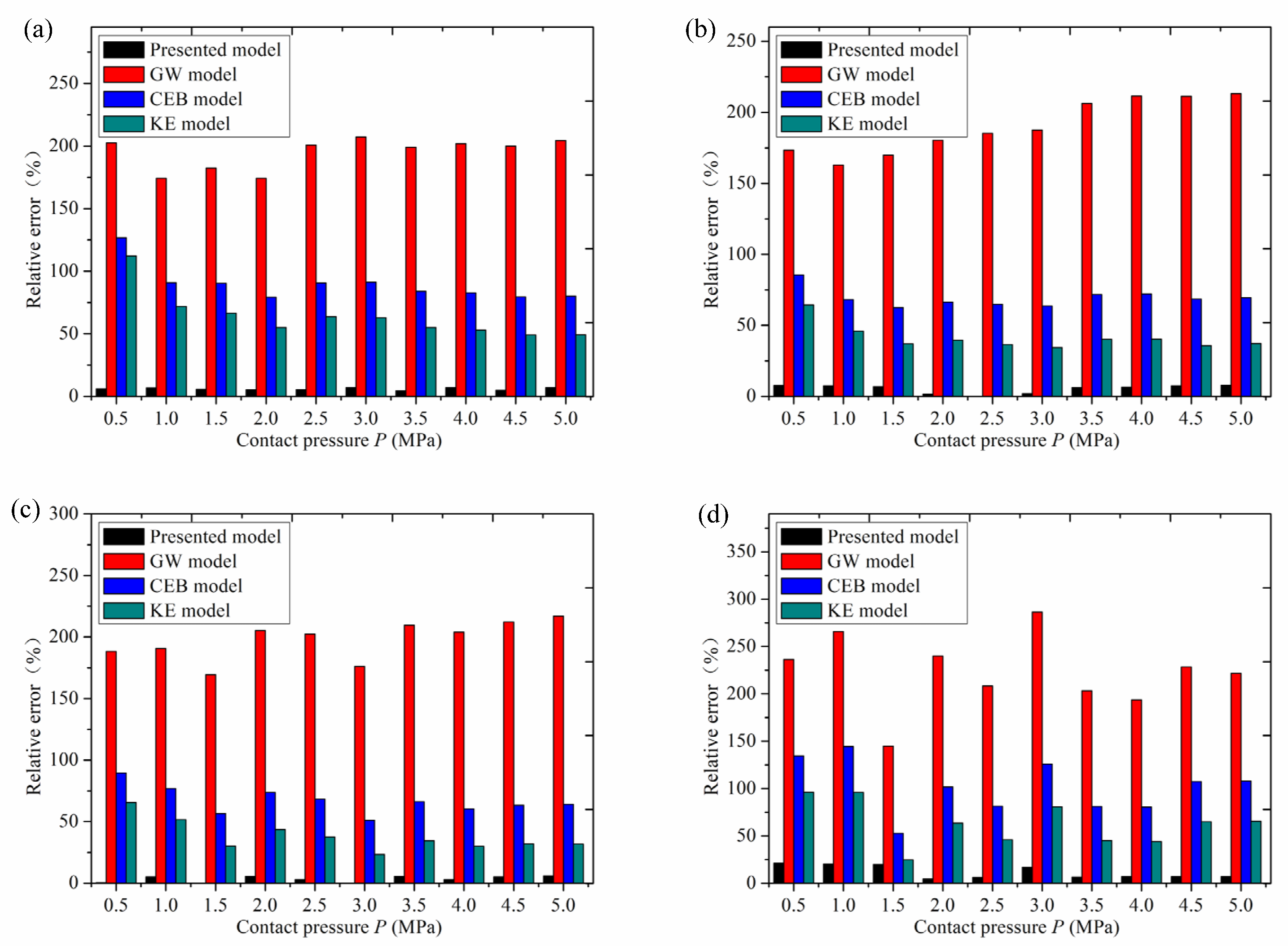
Figure 13 shows the relative error histogram of the experimental value of the normal contact stiffness of rough surfaces with different roughness values compared with the stiffness value of this model, GW model, CEB model and KE model, respectively. As can be seen from the figure, the relative error of the stiffness of the GW model is the largest, the relative error of stiffness of the CEB model and KE model is smaller than that of the GW model, and the error of the new model is the smallest.
The comparison and relative error analysis results of the above models show that the GW model has the largest relative error because the GW model simplifies the contact between two rough surfaces to the contact between a spherical asperity and a rigid plane, and assumes that only elastic deformation occurs in the asperity. Without considering the influence of plastic deformation, it does not conform to the real contact mechanism, resulting in a large error. The CEB model assumes that the volume of the asperity remains unchanged during the contact process, the plastic deformation factor is considered, and the error is smaller than that of the GW model. However, the CEB model assumes that the asperity is in contact with the rigid surface as a spherical asperity, and the model topography assumption is not consistent with the real contact situation, resulting in poor model accuracy. The KE model assumes that the rough surface asperity is spherical asperity, and the deformation of asperity is divided into the elastic stage, elastoplastic stage and complete plastic stage. Compared with the GW model, the error is lower. However, the KE model assumes that the contact of the bonding surface is the contact between a spherical asperity and a rigid plate. This deviates from the real contact condition, resulting in error in the model simulation value. The model proposed in this paper establishes a parabolic cylindrical asperity model by fitting the real rough surface data. This is consistent with the real contact of the bonding surface. In this model, the deformation of asperity is divided into the elastic deformation stage, elastoplastic deformation stage and complete plastic deformation stage. Therefore, the simulation results of this model are better than those of the GW, KE and CEB models.

6. Conclusions

In this paper, the rough surface grinding data were collected, the profile parameters and topography characteristics of the asperity were analyzed, the rough surface data were fit, the asperity profile was resimulated, and the parabola y = nx2 + mx + l cylindrical asperity model was established. After analysis and research, the following conclusions were reached:
  • The rough surface data of grinding were analyzed, and the distribution height of asperity was fitted with the Gaussian distribution function to confirm that the height of asperity obeyed the Gaussian distribution law.
  • The hypothesized model was treated without dimensions and fitted with six plasticity indices to confirm the validity of the model.
  • The experimental stiffness values are basically consistent with the fitting stiffness values of the new model, which verifies the reliability and effectiveness of the new model established for the grinding surface.
  • When the pressure is the same, the normal stiffness increases with the decrease in the roughness value of the joint surface. Roughness affects the contact stiffness between components. In practice, the stability of mechanical equipment can be effectively improved by improving the grinding precision and reducing the roughness of the joint surface.

Author Contributions

Conceptualization and methodology, Y.B.; validation, X.J., F.G. and S.S.; writing—original draft preparation and visualization, Y.B. All authors have read and agreed to the published version of the manuscript.

Funding

This work is financially supported by the National Natural Science Foundation of China (No. 52174154), and the National Natural Science Foundation of China (No. 11802035).

Data Availability Statement

Data is contained within the article.

Conflicts of Interest

The authors declare no conflict of interest.

References

  1. Greenwood, J.A.; Williamson, J.B.P. Contact of nominally flat surfaces. Proc. R. Soc. Lond. Ser. A Math. Phys. Sci. 1966, 295, 300–319. [Google Scholar] [CrossRef]
  2. Chang, W.R.; Etsion, I.; Bogy, D.B. An Elastic-Plastic Model for the Contact of Rough Surfaces. J. Tribol. 1987, 109, 257–263. [Google Scholar] [CrossRef]
  3. Kogut, L.; Etsion, I. Elastic-plastic contact analysis of a sphere and a rigid flat. J. Appl. Mech.-T Asme 2002, 69, 657–662. [Google Scholar] [CrossRef]
  4. Xie, W.; Liu, C.; Huang, G.; Qin, Z.; Zong, K.; Jiang, D. Trans-scale rough surface contact model based on molecular dynamics method: Simulation, modeling and experimental verification. Eur. J. Mech. A/Solids 2023, 100, 105021. [Google Scholar] [CrossRef]
  5. Jamshidi, H.; Tavakoli, E.; Ahmadian, H. Modeling polymer-metal frictional interface using multi-asperity contact theory. Mech. Syst. Signal Process. 2022, 164, 108227. [Google Scholar] [CrossRef]
  6. Kang, H.; Li, Z.-M.; Liu, T.; Zhao, G.; Jing, J.; Yuan, W. A novel multiscale model for contact behavior analysis of rough surfaces with the statistical approach. Int. J. Mech. Sci. 2021, 212, 106808. [Google Scholar] [CrossRef]
  7. Yuan, B.; Wang, Y.; Sun, W.; Mu, X.; Zhang, C.; Sun, Q. Theoretical and experimental study on interface stiffness measurement of rough surface using improved acoustic model. Mech. Syst. Signal Process. 2023, 186, 109839. [Google Scholar] [CrossRef]
  8. Li, W.; Zhan, W.; Huang, P. A physics-based model of a dynamic tangential contact system of lap joints with non-Gaussian rough surfaces based on a new Iwan solution. AIP Adv. 2020, 10, 035207. [Google Scholar] [CrossRef]
  9. Majumdar, A.; Bhushan, B. Role of Fractal Geometry in Roughness Characterization and Contact Mechanics of Surfaces. J. Tribol. 1990, 112, 205–216. [Google Scholar] [CrossRef]
  10. Xie, Y.; Xiao, Y.; Lv, J.; Zhang, Z.; Zhou, Y.; Xue, Y. Influence of creep on preload relaxation of bolted composite joints: Modeling and numerical simulation. Compos. Struct. 2020, 245, 112332. [Google Scholar] [CrossRef]
  11. Shen, F.; Li, Y.-H.; Ke, L.-L. On the size distribution of truncation areas for fractal surfaces. Int. J. Mech. Sci. 2023, 237, 107789. [Google Scholar] [CrossRef]
  12. Yu, X.; Sun, Y.; Wu, S. Analytically decoupling of friction coefficient between mixed lubricated fractal surfaces. Int. J. Mech. Sci. 2023, 255, 108465. [Google Scholar] [CrossRef]
  13. Chen, H.; Yin, Q.; Dong, G.; Xie, L.; Yin, G. Stiffness model of fixed joint considering self-affinity and elastoplasticity of asperities. Ind. Lubr. Tribol. 2019, 72, 128–135. [Google Scholar] [CrossRef]
  14. Chen, J.; Liu, D.; Wang, C.; Zhang, W.; Zhu, L. A fractal contact model of rough surfaces considering detailed multi-scale effects. Tribol. Int. 2022, 176, 107920. [Google Scholar] [CrossRef]
  15. Wang, H.; Jia, P.; Wang, L.; Yun, F.; Wang, G.; Liu, M.; Wang, X. Modeling of the Loading–Unloading Contact of Two Cylindrical Rough Surfaces with Friction. Appl. Sci. 2020, 10, 742. [Google Scholar] [CrossRef]
  16. Yuan, Y.; Xu, K.; Zhao, K. The Loading–Unloading Model of Contact Between Fractal Rough Surfaces. Int. J. Precis. Eng. Manuf. 2020, 21, 1047–1063. [Google Scholar] [CrossRef]
  17. Zhou, C.; Wang, H.; Wang, H.; Hu, B. Three-dimensional asperity model of rough surfaces based on valley–peak ratio of the maximum peak. Meccanica 2021, 56, 711–730. [Google Scholar] [CrossRef]
  18. Shen, F.; Li, Y.-H.; Ke, L.-L. A novel fractal contact model based on size distribution law. Int. J. Mech. Sci. 2023, 249, 108255. [Google Scholar] [CrossRef]
  19. Yu, Q.; Sun, J.; Ji, Z. Mechanics Analysis of Rough Surface Based on Shoulder-Shoulder Contact. Appl. Sci. 2021, 11, 8048. [Google Scholar] [CrossRef]
  20. Zhu, L.; Chen, J.; Zhang, Z.; Hong, J. Normal contact stiffness model considering 3D surface topography and actual contact status. Mech. Sci. 2021, 12, 41–50. [Google Scholar] [CrossRef]
  21. Xie, W.; Liu, C.; Huang, G.; Jiang, D. Numerical and Experimental Study on Rod-Fastened Rotor Dynamics Using Semi-Analytical Elastic-Plastic Model. J. Eng. Gas Turbines Power 2022, 144, 64501. [Google Scholar] [CrossRef]
  22. Zhang, L.; Wen, J.; Liu, M.; Xing, G. A Revised Continuous Observation Length Model of Rough Contact without Adhesion. Mathematics 2022, 10, 3764. [Google Scholar] [CrossRef]
  23. Yu, G.; Mao, H.; Jiang, L.; Liu, W.; Valerii, T. Fractal Contact Mechanics Model for the Rough Surface of a Beveloid Gear with Elliptical Asperities. Appl. Sci. 2022, 12, 4071. [Google Scholar] [CrossRef]
  24. Lv, B.; Han, K.; Wang, Y.; Li, X. Analysis and Experimental Verification of the Sealing Performance of PEM Fuel Cell Based on Fractal Theory. Fractal Fract. 2023, 7, 401. [Google Scholar] [CrossRef]
  25. Zhang, C.; Yu, W.; Yin, L.; Zeng, Q.; Chen, Z.; Shao, Y. Modeling of normal contact stiffness for surface with machining textures and analysis of its influencing factors. Int. J. Solids Struct. 2023, 262–263, 112042. [Google Scholar] [CrossRef]
  26. An, Q.; Suo, S.; Lin, F.; Shi, J. A Novel Micro-Contact Stiffness Model for the Grinding Surfaces of Steel Materials Based on Cosine Curve-Shaped Asperities. Materials 2019, 12, 3561. [Google Scholar] [CrossRef]
  27. Li, L.; Wang, J.; Pei, X.; Chu, W.; Cai, A. A modified elastic contact stiffness model considering the deformation of bulk substrate. J. Mech. Sci. Technol. 2020, 34, 777–790. [Google Scholar] [CrossRef]
  28. Jiang, K.; Liu, Z.; Zhang, T. Research on contact mechanics of a 3D self-affine surface topography using mesh regeneration technology. In Proceedings of the 2022 2nd International Conference on Algorithms, High Performance Computing and Artificial Intelligence (AHPCAI), Guangzhou, China, 21–23 October 2022; pp. 312–318. [Google Scholar]
  29. Bai, Y.; An, Q.; Suo, S.; Wang, W.; Jia, X. An Analytical Model for the Normal Contact Stiffness of Mechanical Joint Surfaces Based on Parabolic Cylindrical Asperities. Materials 2023, 16, 1883. [Google Scholar] [CrossRef]
  30. Nuri, K.A.; Halling, J. The normal approach between rough flat surfaces contact. Wear 1975, 32, 81–93. [Google Scholar] [CrossRef]
Figure 1. Flow chart.
Lubricants 11 00508 g001
Figure 2. (a) White light interference surface topography instrument; (b) specimen.
Lubricants 11 00508 g002
Figure 3. 3D micro-topography of grinding surface.
Lubricants 11 00508 g003
Figure 4. Results of parabolic function fitting of asperity contour.
Lubricants 11 00508 g004
Figure 5. Height distribution of asperity.
Lubricants 11 00508 g005
Figure 6. The hypothetical surface.
Lubricants 11 00508 g006
Figure 7. The surface representation of the 3D model hypothesis.
Lubricants 11 00508 g007
Figure 8. Stiffness at different plasticity indices (a) 0.5; (b) 0.7; (c) 1.0; (d) 1.5; (e) 2.0; (f) 2.5.
Lubricants 11 00508 g008
Figure 9. (a) Grinding machine; (b) contact stiffness test specimen.
Lubricants 11 00508 g009
Figure 10. (a) The test platform; (b) compression module; (c) schematic diagram.
Lubricants 11 00508 g010aLubricants 11 00508 g010b
Figure 11. (a) Sa 0.854 μm; (b) Sa 1.173 μm; (c) Sa 1.391 μm; (d) Sa 1.524 μm.
Lubricants 11 00508 g011
Figure 12. (a) Sa 0.854 μm; (b) Sa 1.173 μm; (c) Sa 1.391 μm; (d) Sa 1.524 μm.
Lubricants 11 00508 g012
Figure 13. (a) Sa 0.854 μm; (b) Sa 1.173 μm; (c) Sa 1.391 μm; (d) Sa 1.524 μm.
Lubricants 11 00508 g013
Table 1. Root mean square error.
Fitting functiony = nx2 + mx + ly = cx3 y = gsin(x)
RMSE 0.0160.0180.117
Table 2. Plasticity index and rough surface engineering parameters.
Ψβσ/R
0.50.03028.75 × 10−5
0.70.03391.60 × 10−4
1.00.04143.02 × 10−4
1.50.04766.57 × 10−4
2.00.05411.144 × 10−3
2.50.06011.77 × 10−3
Disclaimer/Publisher’s Note: The statements, opinions and data contained in all publications are solely those of the individual author(s) and contributor(s) and not of MDPI and/or the editor(s). MDPI and/or the editor(s) disclaim responsibility for any injury to people or property resulting from any ideas, methods, instructions or products referred to in the content.

