Review

A Review of the Mixing Length Theory of Convection in 1D Stellar Modeling
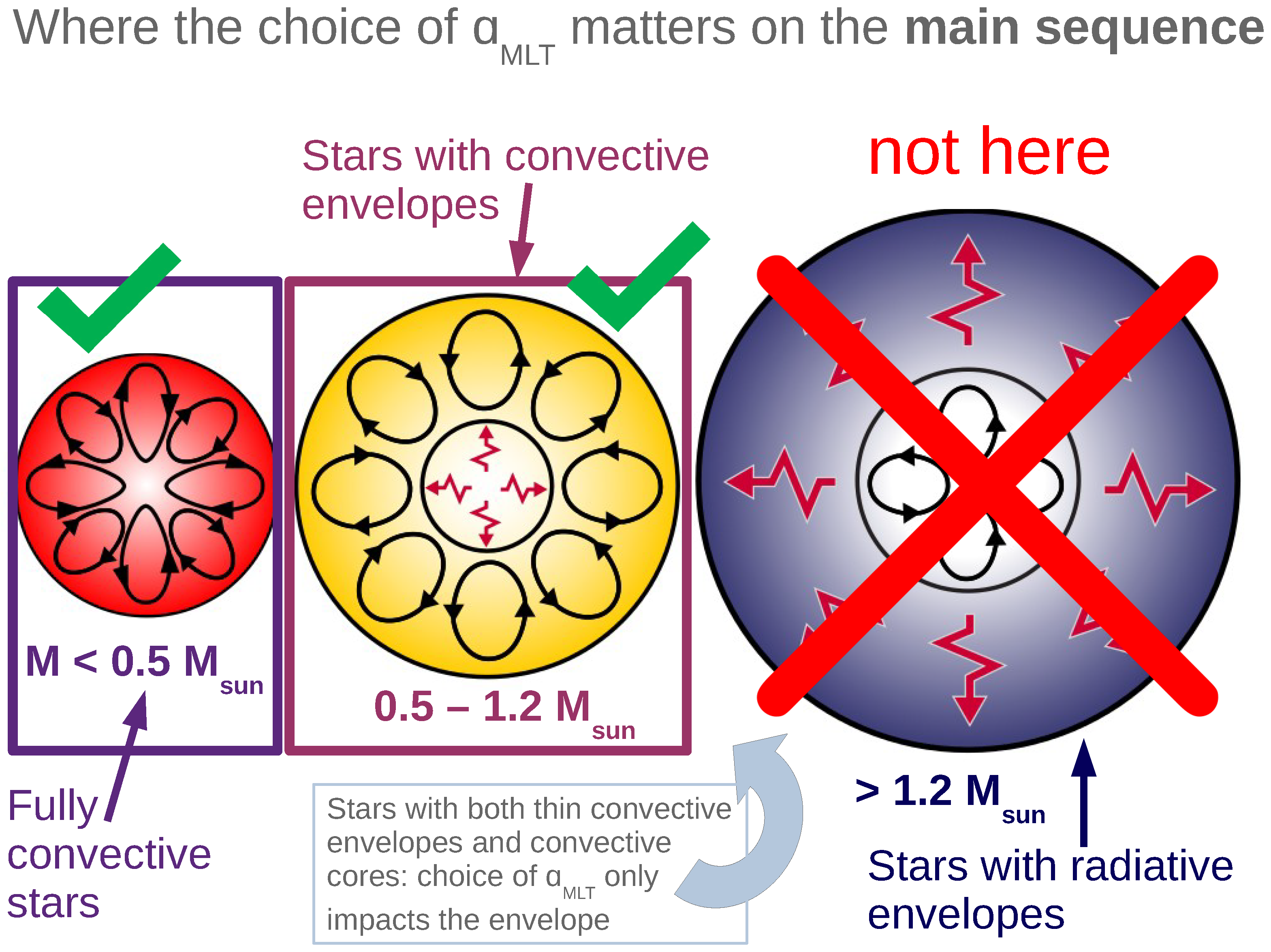
1
Konkoly Observatory, Research Centre for Astronomy and Earth Sciences, Konkoly Th. M. út 15-17., H-1121 Budapest, Hungary
2
CSFK, MTA Centre of Excellence, Konkoly Thege Miklós út 15-17., H-1121 Budapest, Hungary
3
Department of Astronomy, University of Florida, Gainesville, FL 32611, USA
*
Author to whom correspondence should be addressed.
These authors contributed equally to this work.
Galaxies 2023, 11(3), 75; https://doi.org/10.3390/galaxies11030075
Submission received: 16 March 2023 / Revised: 31 May 2023 / Accepted: 4 June 2023 / Published: 16 June 2023
(This article belongs to the Special Issue The Structure and Evolution of Stars)

Abstract

:
We review the application of the one-dimensional Mixing Length Theory (MLT) model of convection in stellar interiors and low-mass stellar evolution. We summarize the history of MLT, present a derivation of MLT in the context of 1D stellar structure equations, and discuss the physical regimes in which MLT is relevant. We review attempts to improve and extend the formalism, including to higher dimensions. We discuss the interactions of MLT with other modeling physics, and demonstrate the impact of introducing variations in the convective mixing length, α MLT , on stellar tracks and isochrones. We summarize the process of performing a solar calibration of α MLT and state-of-the-art on calibrations to non-solar targets. We discuss the scientific implications of changing the mixing length, using recent analyses for demonstration. We review the most prominent successes of MLT, and the remaining challenges, and we conclude by speculating on the future of this treatment of convection.

1. Introduction

The matter of energy transport in stars is notoriously complicated. In particular, the details of convection in the stellar interior are difficult to probe by direct observation and encompass the dominant sources of uncertainty in stellar models (Choi et al. [1], Tayar et al. [2], Cinquegrana et al. [3], Joyce et al. [4]). Even the most specialized one-dimensional (1D) stellar evolution codes must simulate the behavior of stars over enormous ranges in temperature, density, and pressure as well as over evolutionary timescales. Simulations and measurements of convection in non-astrophysical cases indicate the importance of both large- and small-scale motions, and the need to adequately resolve both. When applied to astrophysical problems—which involve timescales ranging from the duration of nuclear processes (fractions of milliseconds) to tens of billions of years, and spatial scales ranging from nuclear cross-sections to thousands of solar radii—this rapidly becomes intractable. Because of the ranges involved, accurately simulating all of these scales simultaneously is computationally infeasible. These requirements therefore demand a simplistic framework for convection. Though convection is an intrinsically three-dimensional, turbulent, non-linear, and time-dependent process, the practicalities of stellar modeling demand that we parameterize convection in a static and one-dimensional way. Mixing length theory (MLT) provides a solution.
The mixing length theory of convection describes the bulk movement of fluids in analogy with molecular heat transfer. By considering a pocket within a convection zone as a discrete “parcel” of fluid, with locally uniform physical characteristics, we may trace its vertical displacement. Assuming the parcel is in pressure equilibrium with its surroundings but not in thermal equilibrium, a relatively hot parcel will move towards a cooler region, and cooler parcels will move towards hotter regions. As hot parcels are under-dense relative to their surroundings, it is a buoyancy force that causes them to rise and expand. Cooler parcels, on the other hand, sink and compress. The characteristic distance over which such a parcel can travel (along a radial line, in one dimension) before losing its locally homogeneous physical characteristics can be thought of as the mean-free path of that parcel, measured in terms of the pressure scale height, d ln ( P ) / d ln ( T ) , of the stratified fluid.
First applied to stellar interiors more than 60 years ago, in an influential paper on solar convection (Böhm-Vitense [5]), the mixing length theory of convection remains the dominant framework for one-dimensional (1D) convective energy transport used in stellar structure and evolution calculations. This longevity speaks not only to its robustness and effectiveness as a formalism, but also to the difficulty of constructing viable alternatives, even in today’s era of exceedingly greater computing resources. With rare exceptions, all modern 1D stellar structure and evolution programs use MLT, or a close variant thereof, for convective energy transport. Popular stellar evolution tools for the low- and intermediate-mass regimes include:
.
ATON Rome Stellar Evolution Code (Ventura et al. [6], Ventura et al. [7]);
.
Bag of Stellar Tracks and Isochrones (BaSTI; Pietrinferni et al. [8]);
.
Cambridge STARS (Eggleton [9]);
.
Code d’Evolution Stellaire Adaptatif et Modulaire (CESAM; Morel and Lebreton [10]);
.
The Dartmouth Stellar Evolution Program (DSEP; Dotter et al. [11]);
.
The Garching Stellar Evolution Code (GARSTEC; Weiss and Schlattl [12]);
.
The Geneva Stellar Evolution Code (GENEC; e.g., Charbonnel et al. [13]);
.
Modules for Experiments in Stellar Astrophysics (MESA; Jermyn et al. [14], Paxton et al. [15,16,17,18,19]);
.
The Monash stellar evolution code (an adaptation of the Mount Stromlo Stellar Evolution code; Lattanzio [20,21], Frost and Lattanzio [22], Karakas and Lattanzio [23]);
.
The PAdova and TRieste Stellar Evolution Code (PARSEC; Bressan et al. [24]);
.
The Yale Rotating Stellar Evolution Code (YREC; Demarque et al. [25]).
Among these, only ATON and CESAM provide an alternative to MLT: the full spectrum of turbulence model of Canuto and Mazzitelli [26] and Canuto et al. [27], discussed further in Section 7.1. For a more thorough overview of stellar evolution codes and their specializations, see the introduction of Cinquegrana et al. [3].
Driven, in part, by ambitious space-based surveys such as Gaia [28], TESS [29], and Kepler [30], by ground-based efforts such as LSST [31], APOGEE [32], LAMOST [33], GALAH [34], and so forth, and by the rich data climate they are generating, there is renewed interest in and understanding of the importance of model-derived fundamental stellar parameters. Given the ubiquitous use of MLT in stellar evolution calculations, we now present a review of 1D convection and its applications, especially to the theory and observation of low-mass (∼0.5–1.0 M ) stars.

2. History

Here we summarize the key milestones in the development and extension of the mixing length theory in its application to stellar interiors.
In 1925, fluid dynamicist Ludwig Prandtl developed a simplified model of Reynolds stress by analogy with molecular heat transfer (Prandtl [35]). This set the precedent for describing turbulent motions using a diffusion approximation, which is a defining feature of all modern-day mixing length theory formulations. Almost 30 years later, Erika Böhm-Vitense developed the first incarnation of mixing length theory for use in models of stars and applied the framework to solar convection (Vitense [36]). Published 70 years ago at the time of writing, Die Wasserstoffkonvektionszone der Sonne, or “The Hydrogen Convection Zone of the Sun”, remains the canonical reference for MLT treatments in models of the Sun and other stars, but it was not until 5 years afterwards that Erika Böhm-Vitense generalized her theory to stars with different effective temperatures, in Böhm-Vitense [5].
Her work was extended by Henyey, Vardya, and Bodenheimer (Henyey et al. [37]), who focused on the formal theory for representing the superadiabatic layers in convective envelopes. This yielded a modified MLT formalism that remains the optimal choice for use in optically thin regimes in stellar structure and evolution calculations. Following this, Cox and Giuli [38] presented an MLT formalism that was ideal for optically thick material.
In 1971, Erika Böhm-Vitense’s husband, Karl-Heinz Böhm, and J. Cassinelli studied MLT in the context of the thin convective envelopes found on white dwarfs (Bohm and Cassinelli [39]). Later that decade, Dmitri Mihalas (Mihalas et al. [40], Mihalas [41]) and Kurucz [42] published studies of radiative transfer models of stellar atmospheres, in connection with sub-surface convection zones characterized by MLT.
The advent of helioseismology (e.g., Basu et al. [43,44]) allowed for deeper understanding of the Sun’s convection zone. In the late 1990s, Demarque et al. [45,46] investigated the superadiabaticity of the Sun and the effects of MLT on the predicted acoustic pressure modes (or p-modes) propagating in the convective cavity. To this day, p-mode asteroseismology remains one of the most powerful tools for characterizing the outer envelopes of low-mass stars, and is a powerful diagnostic for our theoretical treatments of convection.

3. Stellar Structure Context

Here we briefly summarize the principles of stellar structure and evolution, and the thermodynamic quantities necessary to build an intuitive picture of mixing length theory.

3.1. Stellar Structure Equations

In stellar evolution calculations, the equations of stellar structure are solved under the assumptions of conservation of momentum, conservation of mass (or mass continuity), and hydrostatic equilibrium. In the simplest scenario, it is assumed that hydrostatic equilibrium is achieved through the balance of gravitation and pressure. The Eulerian formulation1 of the canonical stellar structure equations is given by Equations (1a)–(1h):
ρ d v d t = P ρ Φ Momentum conservation
2 Φ = 4 π G ρ Gravitation
d P d r = ρ d Φ d r Hydrostatic equilibrium
d M d r = 4 π r 2 ρ Mass continuity
d L d r = 4 π r 2 ρ ϵ ( ρ , T , μ ) Conservation of energy
d T d r = 3 16 π a c κ ρ L r 2 T 3 Radiative energy transport
= G M c p r 2 Adiabatic convective energy transport
d ρ i d t = Q i Nuclear energy generation .
At its core, a stellar structure and evolution code is a polytrope solver. A polytrope is a self-gravitating gaseous sphere, and this physical system provides a reasonable, first-order approximation of an uncomplicated star. A self-gravitating, spherically symmetric ball of fluid can be characterized using the dimensionless Lane–Emden equation:
1 ξ 2 d d ξ ξ 2 d θ d ξ + θ 2 = 0 ,
where ξ can be taken as a proxy for r and θ as a proxy for density ( ρ ). We seek a solution θ ( ξ ) ρ ( r ) . The Lane–Emden equation must be solved under the assumption of an equation of state relating pressure, density, and temperature, one example of which is the ideal gas law; however, temperature can be neglected in the simplest model. The polytropic equation of state usually takes the form P = K ρ 1 + 1 n , where n is the polytropic index and K is a constant of proportionality. Obtaining θ ( ξ ) ρ ( r ) yields the stellar profile, which describes the distribution of matter in the star.
Solving this equation provides a solution for the stellar structure; however, to compute the stellar evolution, we must have a temporal component. In a real equation of state (e.g., the ideal gas law), there is temperature dependence, and the thermodynamic state of the model changes from time step to time step, according to nuclear energy generation. Monitoring how the stellar structure solution—in particular, the outer boundary values for quantities such as effective temperature T eff , luminosity, and radius—changes as a function of time provides us with evolutionary tracks. The key ingredients a user must specify when generating an evolutionary track are the mass, composition, and mixing length of the model. While mass and composition are physical quantities in a way that mixing length is not, all three are equally important in determining the model star’s evolutionary and structural behavior.

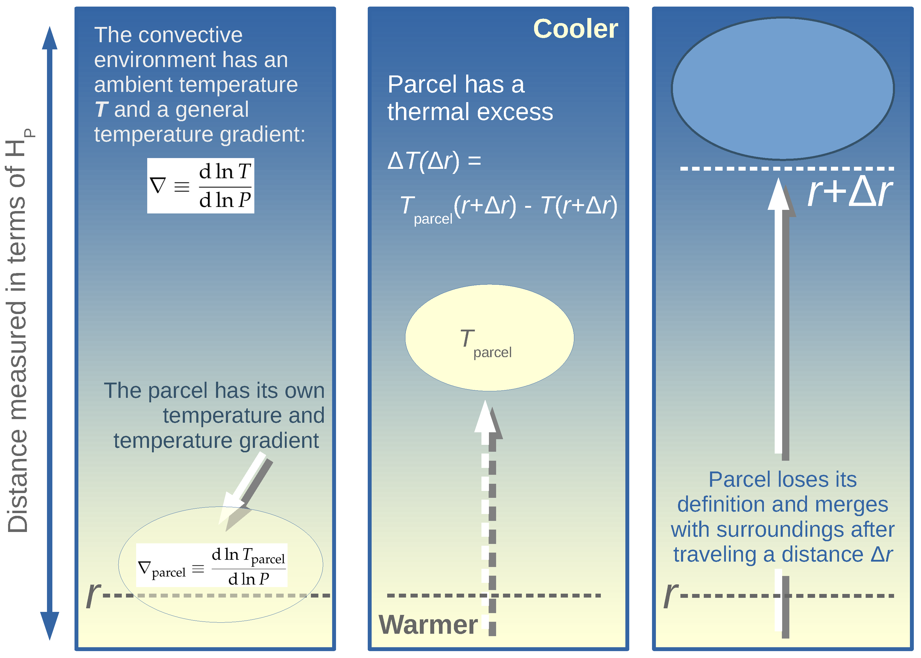
3.2. Thermodynamic Quantities and Convective Stability Criteria

During each time step, the model’s thermodynamic structure must be calculated. This requires knowledge of whether any given radial shell is stable against convection. To evaluate convective stability, we check the Schwarzschild [47] and/or Ledoux [48] criterion.2 The Ledoux criterion for dynamical stability is given by
rad < ad + ϕ / δ μ ,
where ϕ , δ are the partial derivatives of density with respect to temperature and composition, respectively; rad , ad are the radiative and adiabatic temperature gradients, respectively; and  μ is the composition gradient. Under the simplification of homogeneous chemical composition ( μ 0 ), this reduces to the Schwarzschild stability criterion: rad < ad .
When the applicable condition is satisfied, the zone being evaluated is dynamically stable. Dynamically stable regions do not produce convective motions, and so the energy flux is carried out exclusively by radiation (or conduction) in these regimes.
If the convective stability criterion is not met, however, convection will activate and share in the transport of flux (i.e., luminosity or energy). In cases of efficient convection (such as deep core convection—see Section 4), the flux is carried entirely by convection. Stellar evolution calculations invoke MLT in cases where carriage of the flux is shared by radiation and convection.
In this latter case, a useful toy model for mixing length theory is
F conv = 1 2 ρ v c P T λ H P ( T ad )
with
α MLT λ H P ,
where ρ , v , c P represent density, velocity, and specific heat, respectively, and the final term captures the balance of the global temperature gradient, T , against the adiabatic temperature gradient, ad (a more formal derivation is given in Section 6). The definition in Equation (5) is that of the mixing length parameter, or  α MLT . This is a dimensionless parameter, characterizing the “distance,” measured in terms of the pressure scale height H P = d ln ( P ) / d ln ( T ) , that a parcel of convective material can travel.
This α MLT can be thought of in many ways, including as the convective mean-free path (as discussed in Section 1), as a measure of the convective efficiency, or as a pseudo-physical quantity that captures the change in entropy from the base to the top of the convection zone (see end of Section 4). The quantity F conv is determined according to two things: the difference in temperature gradients and the value assigned for α MLT . The suppression or enhancement of surface convective flux can be modulated by α MLT : larger values for α MLT mean that more flux is carried by convection. Changing this value has been shown to impact the predicted surface properties of low-mass stars in ways that should not be ignored (see Section 12).

4. Where Does the Choice of α MLT Matter in Stellar Models?

Stellar modelers typically classify main-sequence stars according to mass, in three main categories: those that are fully convective (stars less than about 0.5 M ; e.g., M dwarfs); those that have radiative cores and convective envelopes ( 0.5 –1.2 M , or stars like the Sun); and those that have convective cores with radiative envelopes (>1.2 M ). Figure 1 depicts the “convective configurations” of main-sequence stars of various mass. Mixing length theory is used to characterize energy transport in stars of all masses and all regions therein, but the choice of α MLT is only important for models in the lower two mass categories, and not in the third. It is also important in models of, e.g., F-type stars, which host a thin convective envelope as well as a convective core, with a radiative zone between them. In this case, MLT is only relevant to the outer convection zone.
The impact of α MLT in mixing length theory is felt only in superadiabatic regions, or regions where the temperature and density gradients align such that higher temperatures correspond to lower densities, causing hot material to rise. This is because the mixing length parameter is tied to a temperature excess that only exists in regions where the flux is carried by a combination of radiation and convection (whereas the flux is carried entirely by convection in the case of convective stellar cores, where the temperature gradient is nearly adiabatic; see Section 6 for more detail).
Superadiabatic regions of low-mass stars include surface convection zones, sub-surface convection zones, and (later in their evolution) red giant envelopes. In intermediate- to high-mass stars, conditions may also produce intershell convection, or localized, interior pockets of convection situated between the core and the envelope.
Importantly, convection in the stellar core is not a case of superadiabatic convection. While convection at the surface is very inefficient, conditions in the core locally approximate an isentropic3 environment, meaning core convection is adiabatic. The standard prescription for energy transport by convection in adiabatic regimes is given by Equation (1g). This can be written (in Lagrangian form, i.e., m rather than r coordinates) as
d T d m = T P G m 4 π r 4 ,
where ∇ represents the general temperature gradient (see Equation (7.32) and surrounding discussion in Kippenhahn and Weigert [52]). Note that the form of ∇ is key: in the deep interior, = ad ; in the regions where MLT applies, ∇ is instead given by the solution to Equation (4).
Referring again to Equation (4), we see how mixing length theory’s key parameter, α MLT , can be conceptualized as a measure of convective efficiency, with higher values corresponding to the statement that a larger amount of flux is carried by convection. Changes to the stellar structure induced by changes in α MLT will, therefore, be most significant when convective efficiency is low.
Within a superadiabatic convective region, there is still a differential in the efficiency of convection as a function of depth4. While the deepest portion of the outer convection zone is nearly adiabatic, or asymptotically adiabatic, the top of the convective envelope is not. The difference in entropy between these regions is also captured by α MLT .

5. Limitations and Physics Not Captured by MLT

Mixing length theory requires a number of naïve—and in some cases, outright incorrect—physical assumptions. First of all, MLT models an advective process, using a diffusive approximation. Advective processes are those that transport material or energy through the bulk motion of fluids, whereas MLT supposes that particle-like fluid parcels diffuse through the region, to redistribute heat. In the physical world, fluids and particles behave quite differently, and radiative hydrodynamics has shown that the concept of a homogeneous unit of convective material sustained over any appreciable distance is not valid: convection proceeds via a continuum of constantly changing upflow and downflow channels. Likewise, MLT treats convective boundaries as if they are rigid. In reality, convective boundaries are permeable, flexible, and subject to the inertia of convective motions carrying convective plumes across the convective–radiative boundary. Local mixing occurs in these regions, and MLT cannot account for this.
Another simplification supposed by MLT is that fluid parcels travel along strictly vertical paths: this limitation is primarily due to the 1D aspect of the formulation. In physical convection, there is continuous shearing, fragmentation, reorientation, and deletion of the flow channels: none of these features can be captured using a formulation that relies on strictly radial displacements. It should also be emphasized that standard MLT is not time-dependent, which means that it cannot capture any physics happening faster than the convective turnover time. In standard treatments, convective regions are assumed to be instantaneously mixed over one evolutionary time step.
On the issue of flow channels, MLT fails to account for the fact that, in physical convection, there is asymmetry between upflows (hot material rising) and downflows (cool material falling). Taking, for example, the surface of the Sun or 3D simulations thereof, we observe that a network of broad, spot-like convective cells with higher temperatures is demarcated by a series of interconnected, cooler downflow lanes. The surface area is dominated by plasma flowing upward, which expands as its density drops, and this material travels in the same direction as the density gradient; however, the same is not true of the down-flowing material, which travels against the density gradient, and generates turbulence in the process. To satisfy both conservation laws and the density gradient, the upflows lose mass to the downflows, and the downflows accumulate contributions from the upflow lanes at many different radial and density coordinates.
Because the upflows carry material that is uniformly from the deep interior of the convection zone to the surface, the process is largely isentropic. There is no such uniformity in the downflow lanes, however: the material in these lanes has a range of entropies, and it is also denser. The downflows therefore cause turbulence, have higher speeds than the upflows, and occupy a smaller area than the upflows. These conditions result in the inward (towards the interior) transfer of kinetic energy, a process known as negative kinetic flux. Negative kinetic flux is a physical property of convective plasma that classical MLT cannot capture, though some modern extensions and revisions of MLT have attempted to incorporate this feature (see Stein and Nordlund [53] for a detailed discussion of 3D plasma physics).
It is likewise important to recognize that the mixing length parameter, α MLT , of most MLT formulations is only loosely connected to any physical property of a star; it is often thought of as a free, numerical parameter. The mixing length is, however, related to the entropy jump between the asymptotically adiabatic portion of the convection zone (where convection is most efficient) and the top of the convective envelope (where it is least efficient). Although neither this entropy jump nor the density gradient, size, or depth of the convective envelope is a readily observable feature of a star, these features can be probed indirectly using asteroseismology. It is thus necessary to calibrate α MLT directly, and this is most easily done using observations of our nearest star—a point to which we return in Section 10.

6. Mixing Length Formulation

We reproduce here a standard derivation for the amount of flux carried by convection, modified from derivations presented in Cox & Giuli’s Principles of Stellar Structure, Kippenhahn and Wieger’s Stellar Structure and Evolution, Cassisi & Salaris’ Stars and Stellar Populations, and notes compiled by Matteo Cantiello and Yan-Fei Jiang (priv. comm.).
The pressure scale height, H p , is a measure of the distance over which the total pressure, P = P gas + P rad , changes by a factor of 1 / e . Under the assumption of hydrostatic equilibrium, the definition
d ln P d r ρ g P = 1 H P
holds.
MLT’s canonical “parcel of fluid” is taken to be in pressure, but not thermal, equilibrium with its surroundings. We next define (1) the average (ambient) temperature gradient of the fluid, with respect to the pressure of all matter at some r, and (2) a temperature gradient of the fluid parcel itself, also taken with respect to the total pressure. Let the former be given by
d ln T d ln P ,
and the latter by
parcel d ln T parcel d ln P ,
where T and T parcel are the average (ambient) temperature and the temperature of the parcel, respectively. This scenario is depicted in Figure 2.
By first-order Taylor expansion, the difference between the parcel’s temperature and the ambient temperature at some radial shift Δ r can be expressed as
Δ T ( Δ r ) = T parcel ( r + Δ r ) T ( r + Δ r ) Δ r d T parcel d r d T d r .
Assuming that the temperature change over Δ r is small, T T parcel , and so
Δ r d T parcel d r d T d r Δ r T d ln T d r d ln T parcel d r .
Using the chain rule and the definition from Equation (7), we can rewrite
d ln T d ln P = d ln T d r d r d ln P = d ln T d r H P .
We may now substitute the definitions from Equations (8) and (9) into Equation (11), yielding
Δ T ( Δ r ) = Δ r T H P ( parcel ) .
We note that the moving parcel may well exchange heat with its environment, and so parcel is a function of the rate at which this exchange takes place. However, the assumption that the parcel does not exchange heat with its surroundings—i.e., that it is moving adiabatically—is a reasonable and simplifying assumption for stellar conditions. In this case,
parcel ad = d ln T d ln P ad .
Take careful note of the difference between Equations (14) and (8): these are not interchangeable. The adiabatic temperature gradient, ad , and the average or ambient temperature gradient, ∇, are not, in general, the same. We also do not necessarily know the definition of ∇ in a convective region. Substituting parcel for ad and combining with Equation (13) yields
Δ T ( Δ r ) = Δ r T H P ( ad ) .
Meanwhile, the convective flux transported by a parcel of fluid moving upwards with velocity v over some distance λ is given by
F conv = 1 2 ρ v c P d T d r ad d T d r λ ,
where ρ is density, c P is specific heat, and the factor of 1 2 emerges from the assumption that half of the material in a given layer is rising while half is falling (see Salaris and Cassisi [54] for more discussion of how this formula arises). Given the relationship
d T d r = T H P d ln T d ln P = T H P
and Equation (13), we have
F conv = 1 2 ρ v c P T H P ad T H P λ .
Rearranging, we see that Equation (4),
F conv = 1 2 ρ v c P T λ H P ( T ad ) ,
describing the toy model introduced in Section 3, emerges.
We return briefly to stars with convective cores, as discussed in Section 4: in convective cores, where convection is efficient, conditions are nearly isentropic, and the general temperature gradient is an adiabatic temperature gradient. In this case, ( T ad ) = ( ad ad ) = 0 , so we can see that the choice of α MLT does not matter in this situation.

Specific Formulations

There are several implementations of MLT, some of which are more appropriate for particular physical scenarios. One of the most commonly used today is the Cox and Giuli [38] prescription, which assumes high optical depth and no radiative losses, as does the original formulation of Böhm-Vitense [5]. The methods of Henyey et al. [55], Mihalas et al. [40], and Kurucz [56] all provide extensions of MLT to work in optically thin regimes. To use MLT in regimes where electron degeneracy and pressure ionization are relevant, as in the convective envelopes of white dwarfs, the Bohm and Cassinelli [39] extension is most appropriate.
The use of time-dependent convection has its origins in the study of stellar pulsations, beginning with the work of Unno [57] and Gough et al. [58] in adapting the mixing length formulation to model the interaction of the turbulent velocity field with radial pulsations (see Houdek and Dupret [59] for a detailed review of this topic). Recent innovations in time-dependent convection include implementing the model of Kuhfuss [60] in MESA (Jermyn et al. [14]), which reduces to the standard Cox and Giuli [38] treatment over long timescales.

7. Alternatives and Extensions

The simplistic assumptions on which mixing length theory is based have long cried out for a more sophisticated and realistic formulation. Numerous authors have suggested potential changes to the mixing length formalism, including the inclusion of non-local elements, use of a more consistent picture of the turbulent dissipation, use of more physically motivated parameterizations, and/or use of more complex calibrations.

7.1. Alternative 1D Formulations

Improvements to MLT must balance increased sophistication against the need to remain implementable in one-dimensional stellar evolution models. Many attempts have been made; however, while such modifications often provide better answers in particularly challenging regions of stellar evolution (e.g., time-dependent convection in late stages of nuclear burning for massive stars), they are often discussed only in the local context of a particular problem. The comparative simplicity and wide applicability of the standard mixing length formalism has thus far prevented any wide adoption of a significantly different alternative. We discuss a few alternative formulations of the mixing length theory here, although we acknowledge that there is a wider body of work in this field than we can adequately document here (see, e.g., Houdek and Dupret [59]).
One early challenge to the mixing length formalism was the fact that its purely local formulation meant that it did not accommodate convective overshoot: MLT provided no way to get convective regions to overshoot into adjacent, formally stable radiative regions, even though observations of real stars seemed to demand some such process (Gough [61], Renzini [62], Grossman and Narayan [63]). Attempts have been made to recompute the theory in a non-local way, by including additional convective terms Kuhfuss [60], Eggleton [64], Xiong [65,66,67], Grossman [68], but such expansions rapidly develop a significant number of extra terms as they try to include higher-order effects.
There are classes of modified mixing length models that can, in theory, address other challenges, including time-dependent effects in a pulsating star (Gough [61]), the impact of composition gradients, representation of the depth dependence of rotation and magnetism (Ireland and Browning [69]), and so forth. Practically, however, such work has been limited to specific problems addressed on an individual basis, rather than leading to a true overhaul of the underlying framework.
There have also been more explicit attempts to include a physical description of turbulence in the parameterization of convection. In the inviscid interior of a star, it is expected that a wide spectrum of turbulent eddies contribute to the convective flux (Canuto and Mazzitelli [26], Marcus et al. [70]), rather than the single eddy assumed by the standard mixing length theory. This change in the treatment of energy transport corresponds to differences in the flux carried and the resulting temperature structure (Canuto et al. [27]). This model, known as full-spectrum turbulence, has been adopted in some stellar evolution codes, including CESAM [10] and ATON [6].

7.2. Extensions to 3D

More recently, as three-dimensional simulations of convection have improved, researchers have attempted to use these simulations to constrain the mixing length in a way that more realistically represents the physics of convection. Such simulations can incorporate not only the local and static mixing length, but information on the global derivatives, asymmetries between upflows and downflows, the larger-scale properties of the star, and transverse versus radial differences (Arnett et al. [71]). For reasons likely related to the physics of turbulent dissipation (Arnett et al. [72]), most such simulations tend to find that the value of the mixing length should vary only slightly with the composition, luminosity, and surface gravity of the star (Trampedach et al. [73], Magic et al. [74], Sonoi et al. [75]). However, some authors have attempted to better reproduce the temperature stratification (T- τ ) relations in the three-dimensional simulations (Tanner et al. [76], Salaris and Cassisi [77], Mosumgaard et al. [78], Zhou et al. [79]). Still others have attempted to incorporate additional physical information by calibrating the mixing length parameter directly to the entropy profile (Spada and Demarque [80], Spada et al. [81]).
While trends between α MLT and other global properties (e.g., metallicity) from 3D simulations often proceed in the same direction as the trends implied by calibrations of the mixing length in 1D stellar models to match observations of stars (Bonaca et al. [82], Creevey et al. [83], Tayar et al. [84], Joyce and Chaboyer [85,86], Viani et al. [87]), they rarely agree quantitatively. In particular, there is a large discrepancy in magnitude: 1D-to-observational calibrations suggest, in some cases, the need for a variation in α MLT that is a factor of 10 larger than suggested by 3D simulations. One may compare, e.g., Joyce and Chaboyer [86] to Trampedach et al. [73] on this issue. This suggests either a need for improvement in three-dimensional simulations—for example, by extending their temperature and density domains, or by extending their timescales—or the need for additional corrections to the physics of 1D stellar evolution calculations that are currently impacting the inferred mixing length (Choi et al. [1], Valle et al. [88]). We expect both the 3D and 1D communities will continue their efforts to search for a consensus method that brings the two sets of models into agreement.

8. Standard 1D MLT and Its Interplay with Other Modeling Physics

In addition to the challenges related to the mixing length by itself, stellar modeling relies upon a large number of other physical inputs, including formulations of convective overshoot, opacities, equations of state, the treatment of diffusion, nuclear reaction rates, and so on, and the interplay between α MLT and these other physical assumptions must be considered. While entire articles have been written on each of these options, their associated uncertainties, and their respective impacts on stars of various masses and evolutionary states, our focus here is on how these other physical options interact with the mixing length.

8.1. Atmospheric Boundary Conditions

The creation of a stellar structure model is, in essence, a boundary value problem, where choices about the outer boundary condition will have a significant impact on the resulting solution. Unfortunately, the outer boundary is where radiation begins to escape the star. This is precisely where the assumptions of stellar interiors begin to break down, and where analytic solutions accumulate error. Most modelers deal with this problem by assuming a relationship between the temperature and optical depth in this region (i.e., a T- τ relation): this can be an analytical expression (e.g., Eddington, Krishna Swamy [89], Ball [90]) or a table of values sourced from more sophisticated stellar atmosphere calculations that better include some of the physics of radiative transfer and loss (Kurucz [56]), (Castelli and Kurucz [91]), (Hauschildt et al. [92]). These choices change the structure of the model in the same region that is affected by the mixing length superadiabatic outer layers of the star, and so the chosen atmospheric boundary conditions will change the mixing length. This effect is most obvious in red giant stars, due to their larger convective envelopes. The mixing length is sensitive to both the atmospheric relation adopted and the optical depth in the atmosphere at which the boundary is set (Choi et al. [1]).
We note that stellar atmosphere calculations also require a choice of mixing length (Gustafsson [93]), though the choice of the mixing length in the atmosphere models is generally found to have only marginal impact on their physical predictions (e.g., abundances inferred; Song et al. [94]); however, the mixing length chosen in stellar atmosphere models is rarely forced to be the same as the mixing length chosen in the stellar evolution models. Generally, this inconsistency is assumed not to matter, and the choice to ignore it can be reconciled in a framework where the mixing length is viewed as a tuning parameter accounting for other physical inconsistencies; however, it is more difficult to ignore this inconsistency in a framework where the mixing length is thought to capture something physical about convection.
There are also arguments that three-dimensional simulations provide a better estimation of the relationship between temperature and optical depth, and that these should be used as boundary conditions in lieu of the standard one-dimensional atmosphere models (Trampedach et al. [73], Magic et al. [74], Tanner et al. [76]). Attempts have been made to implement these boundary conditions in a way that takes into account the temperature, metallicity, and luminosity of the star (e.g., Mosumgaard et al. [78,95]); however, in general, the effects on the stellar temperature and assumed mixing length have been smaller than expected (generally on the order of tens of Kelvin; Tanner et al. [76], Mosumgaard et al. [95]).

8.2. Convective Boundaries

Designing stellar models requires assigning the conditions for convection. This involves a choice between the Schwarzschild and Ledoux criteria for convective stability (see Section 3.2), as well as a choice in the mathematical and numerical approach to locating the convective–radiative boundary (or boundaries). While these choices are arguably most important for convective stellar cores (e.g., Pedersen et al. [96])5, they can nonetheless carry significant implications for convective envelopes as well—for example, dredge-up events and nucleosynthetic yields from TP-AGB stars are highly sensitive to these conditions (Cinquegrana et al. [3], Karakas et al. [97]). As such, there are important choices to be made about the physics of the lower boundary of the surface convective zone, where the local temperature gradient is not as close to adiabatic as the temperature gradient near the core and interactions with the mixing length can occur. This is the location of a process sometimes referred to as convective undershoot.
Early work with the mixing length formalism suggested that the Schwarzschild criterion was more likely to be appropriate for setting this boundary (e.g., Grossman and Narayan [63]). Further work has been consistent with that result, indicating that while boundaries tend to be instantaneously consistent with the predictions of the Ledoux criterion, over time they will mix in additional material (Paxton et al. [15]) through processes such as entrainment or oscillatory double diffusive convection (Mirouh et al. [98]), until they grow to the size predicted by the Schwarzschild criterion (Anders et al. [51]).

8.3. Opacities

There are numerous physical assumptions that impact the detailed structure and temperature profiles of the model, meaning that they change our expectations for a solar model and, therefore, the mixing length required to reproduce the properties of the Sun at the solar age (see Section 10). We discuss this here in the context of opacities, but an analogous discussion could be imagined for composition, including individual abundance variations (Pietrinferni et al. [99], Beom et al. [100]), the treatment of diffusion (van Saders and Pinsonneault [101]), and any similar assumption that affects the superadiabatic layers.
Opacity in the stellar interior is generally treated in a simplistic way, in which one assumes an abundance for each element present in the star and reads in a table corresponding to that composition. The table contains an estimate of the Rosseland mean opacity for the prescribed mixture as a function of density and temperature. This is then used to compute how much energy can be carried by radiation. The radiative flux, in turn, helps determine which regions will convect and what the temperature and density of those regions will be: this means that changing the opacities will result in small changes to the estimated radius and surface temperature of the star at any particular time. Since calibrations of the mixing length in stellar models are generally done to fit a particular radius and temperature at a particular time, calibrated models with different opacities will require different mixing lengths, and these differences in mixing length will propagate into differences in the evolutionary timescale, pulsations, and nucleosynthesis (Cinquegrana and Joyce [102]).

8.4. Magnetic Fields

Resolved studies of the solar surface make clear that magnetism, and particularly the concentration of the magnetic field, can impact the local properties of convection (e.g., Roudier et al. [103]). This sort of spatially resolved behavior is, however, challenging to reproduce with one-dimensional stellar evolution models. Originally, such effects were expected to be unimportant, and were therefore ignored: however, this is no longer the case for all stars. In particular, large regions of concentrated magnetic field have been observed on a variety of young stars, on M dwarfs, and on rapidly rotating evolved stars, including the sub-sub-giants (e.g., Gosnell et al. [104], Libby-Roberts et al. [105]). It is now understood that magnetism in these regions influences the surface convective flux, and that these effects can be parameterized in a way that mimics the behavior of the mixing length (e.g., Ireland and Browning [69]).
The magnetic field is thought to act in some cases as an additional magnetic pressure or energy density term that blocks the transport of flux through certain spatial regions, and this effect has been parameterized in some 1D stellar evolution codes (e.g., YREC, Somers and Pinsonneault [106]; MESA, Jermyn et al. [14].) One of the simplest ways to incorporate this effect is by lowering the effective mixing length of the star, which will tend to inflate the star in much the same way as surface magnetism. This inflation increases consistency with the larger-than-expected observed radii of M dwarfs in binary systems (Chabrier et al. [107], Somers and Pinsonneault [108]).
More sophisticated analyses can self-consistently incorporate the effects of magnetism into a modified mixing length theory (Feiden and Chaboyer [109]), or add corrections for the spatial inhomogeneities of star spots (Somers et al. [110]); however, all of these tend to alter the structure in a manner similar to direct alterations to the mixing length. This highlights the complex nature of the mixing length: while clearly a nonphysical parameterization, its values may also point to physical changes in the properties of convection and its interactions with the physics of the stellar interior.

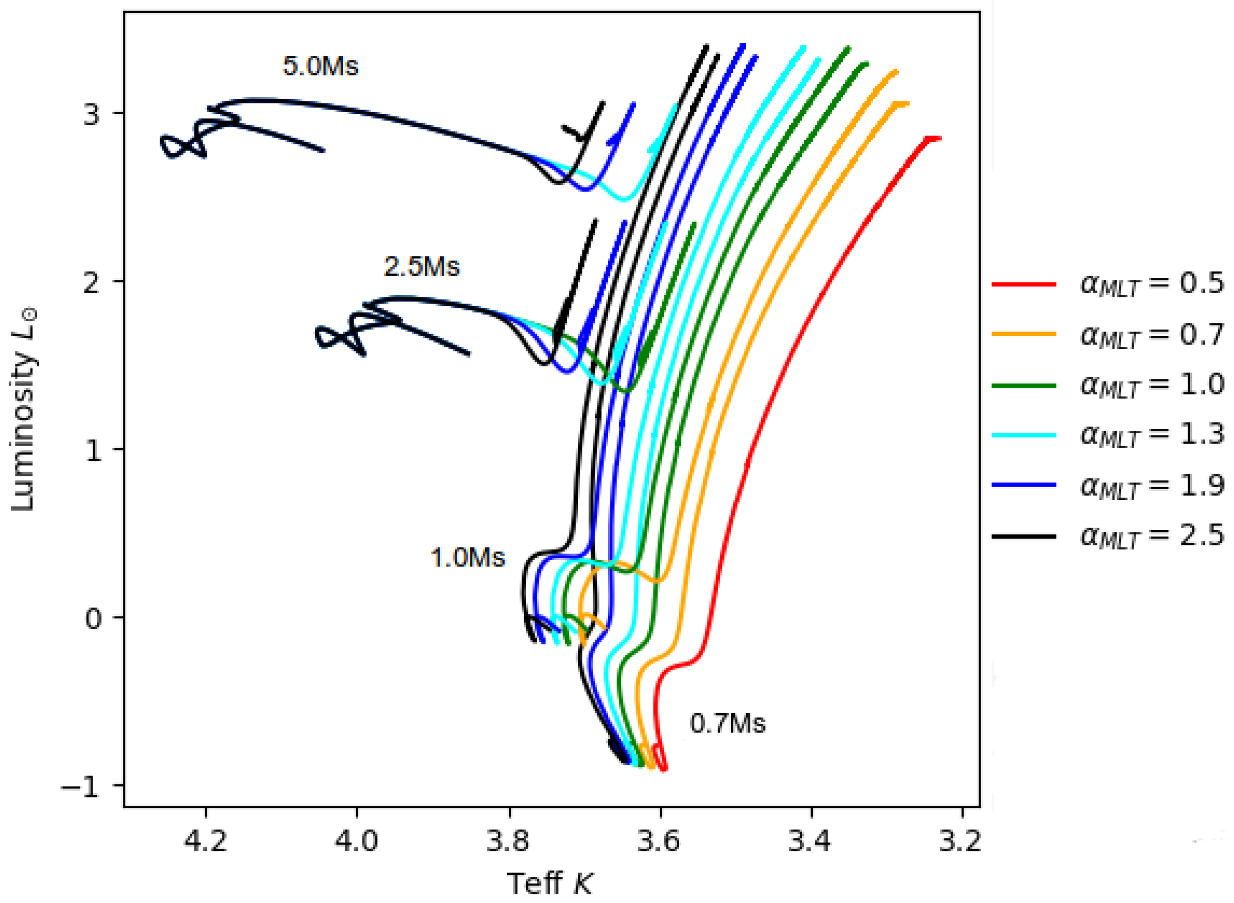
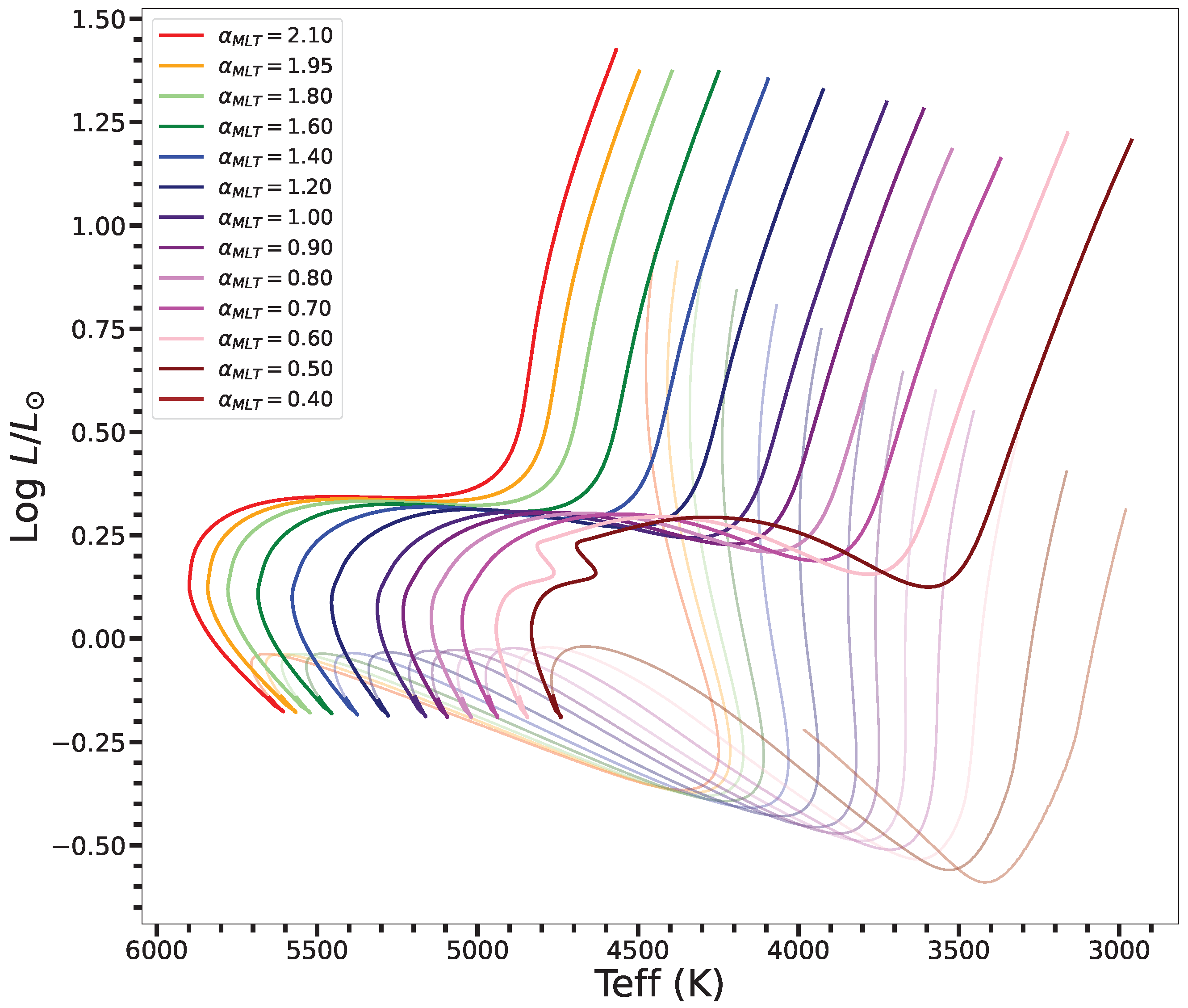
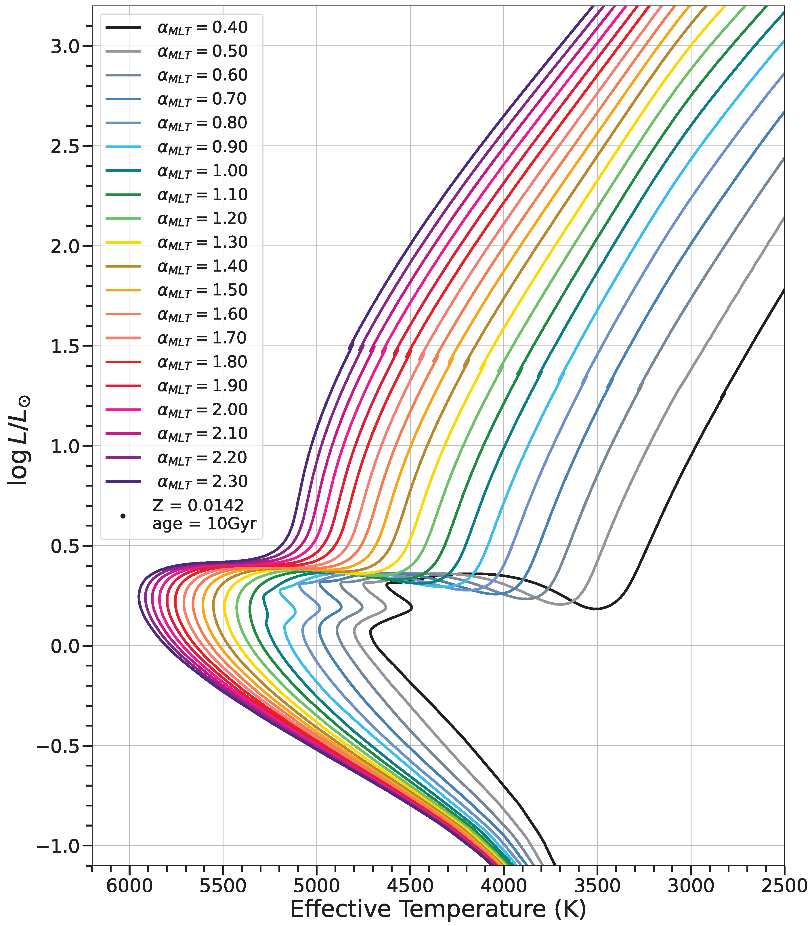
9. What Does Changing the Mixing Length Do in Stellar Models?

The effects of changing the value of α MLT assigned in stellar evolution calculations performed using the Dartmouth Stellar Evolution Program (DSEP; Dotter et al. [11]) are shown in Figure 3. We note first of all that the effect of varying α MLT is itself mass-dependent, with tracks at 2.5 or 5 M showing no change along the main sequence with varying α MLT , whereas those at 1.0 and 0.7 M show a shift towards cooler temperatures with decreasing α MLT : this is because, above a mass of approximately 1.2 M , the structure of the star switches from hosting a convective envelope on the main sequence to hosting a radiative envelope, as explained in Figure 1. As changes to the mixing length will only affect superadiabatic regions with inefficient convection, changing α MLT for models that only exhibit core convection will have no impact. However, we also observe that the effects of changing α MLT begin to manifest for the higher-mass tracks after the main sequence turn-off: this corresponds evolutionarily to the development of a convective envelope, which introduces into the model a region of inefficient convection where MLT applies. We see here that lowering the value of α MLT results in an extension of the subgiant phase, causing it to both lengthen in duration and shift towards cooler temperatures, for the 2.5 and 5.0 M tracks.
For the groups of 1.0 and 0.7 M tracks, changes to α MLT will have an impact throughout their main sequence, subgiant, and red giant evolutionary phases, as a convective envelope persists throughout these phases. Another observation is that changes to α MLT are not linear: the temperature difference between tracks with α MLT = 2.5 vs α MLT = 1.9 is much smaller, in both mass cases, than the difference in temperature caused by a change from, e.g.,  α MLT = 0.5 to α MLT = 1.0 . Intuitively, this is because the impact of changing the efficiency of convection is greatest when the efficiency is low.
In Figure 4, we take a closer look at the 1 M case. The tracks in this figure were computed with MESA rather than DSEP, and variations in the mixing length from α MLT = 0.4 —a value suitable for some M dwarfs (cf. Mann et al. [111])—to α MLT = 2.1 , which is slightly greater than MESA’s default (solar) value, α MLT , MESA default = 2.0 . The same trends observed for the 1.0 M case in Figure 3 are visible here, including:
(1)
The shift towards cooler temperatures with lower α MLT ;
(2)
The difference in effect of a 10% change in α MLT at, e.g.,  α MLT = 2.1 , compared to α MLT = 0.8 ;
(3)
The extension of the subgiant branch in duration, and towards cooler temperatures, with decreasing α MLT ;
(4)
The negligible impact on luminosity.
We note an additional feature in the tracks with the lowest mixing length values: a hook emerges near the end of the main sequence for 1 M tracks with α MLT = 0.4 and 0.5 , which corresponds to the development of a convective core—a feature that would not normally be present in a 1 M model, but which emerges in this case, due to the suppression of convective flux at the surface of the model, and the inward propagation of those effects to the stellar interior. The impact of suppressing convective flux to this degree is significant enough to cause a structural realignment throughout the stellar model—specifically, an inflated radius—which results in a non-standard convective structure for the solar-like tracks with α MLT < 0.6 .

Impact on Isochrones

Isochrones—from iso meaning “single” and chronos meaning “time”—are models that represent a snapshot in time as a function of stellar mass. Whereas stellar tracks depict the time-evolution of a single star of particular mass, isochrones are constructed by interpolating over grids of stellar tracks, each of which has a different initial mass but otherwise identical input physics. As stars of different masses evolve at different rates, points of equal age will occur during different evolutionary stages for different tracks. The curve connecting these equal-aged points across masses is the isochrone. For a more rigorous discussion of how these equal-aged points are defined, we refer the reader to Dotter [112], who provides a description of the Equal Evolutionary Point, or EEP, method.
Figure 4. MESA: all one solar mass, range of MLT values. Other assumptions: photosphere tables for atmospheric boundary conditions and the Asplund et al. [113] solar abundance scale. The pre-ZAMS evolutionary tracks are printed in fainter colors to avoid crowding and overlap with the ZAMS-RGB tracks. Note that in the case of α MLT = 0.40 , the model failed before reaching the ZAMS.
Galaxies 11 00075 g004
It is well known that changes to the physical assumptions of the constituent stellar tracks will change the morphology of the isochrones, especially in mixing-sensitive regions, such as the main sequence turn-off (MSTO) and subgiant branch (e.g., Joyce and Chaboyer [85]), (Somers et al. [110], Song et al. [114]). In publicly available, pre-computed isochrone databases, such as MIST (MESA Isochrones and Stellar Tracks; Choi et al. [115]), the user can specify the composition of the tracks. Occasionally, it is also possible to specify other physics, such as a degree of alpha-element enhancement (as in DSED, the Dartmouth Stellar Evolution Database; Dotter et al. [11]), the degree of overshooting, mass loss, or inclusion of heavy element diffusion (as in BaSTI: Bag of Stellar Tracks and Isochrones; Pietrinferni et al. [116]), and/or whether the underlying models are rotating (e.g., MIST). Synthetic photometry for many observational systems is also available in many isochrone databases.
However, there is no publicly available isochrone database that permits the variation of α MLT . Figure 5 shows the effect of variation in α MLT for a set of isochrones whose ages, compositions, and other physical assumptions are otherwise identical. As Figure 4 would suggest, the impact of lowering α MLT in the constituent stellar tracks propagates into the isochrones, with ultra-low- α MLT models exhibiting a convective core at lower masses than would be expected under typical physical assumptions. We likewise observe the shift towards both lower effective temperatures and greater temperature sensitivity with decreasing α MLT .

10. Solar Calibration of α MLT

Because the mixing length has neither an observable counterpart in real stars nor an analog in 3D convection simulations, we must "guess" its value. Canonically, the value of the mixing length is determined by a method known as solar calibration (e.g., Charbonnel and Lebreton [117]). In this process, α MLT is iteratively adjusted in a solar model, until the model’s temperature, luminosity, radius, and other observationally constrained features (e.g p-mode asteroseismic spectrum) are reproduced to precisions of (ideally) at least 1 part in 10 5 at the solar age. Historically, the Sun was the only star with a sufficient number of independent observational constraints and sufficient precision on those constraints to make this calculation feasible.
Differences in both algorithms and physical assumptions across stellar evolution codes mean that the “solar-calibrated mixing length” is not a universal concept. The value of α MLT , must be independently determined within each stellar evolution code, and again for each set of physical assumptions. For example, α MLT , will, in general, be higher for solar models that incorporate heavy element diffusion than for solar models that do not, and will differ at the level of at least 10 %, depending on the choice of atmospheric boundary conditions. Table 1 of Joyce and Chaboyer [85] and Section 1 of Viani et al. [87] provide clear demonstrations of the degree of variance in α MLT , in the context of different input physics within the same stellar evolution code (DSEP and YREC, respectively). Similarly, Cinquegrana and Joyce [102] demonstrate that the difference between using a “default” solar value (calibrated to some arbitrary set of input physics) and using α MLT , from a solar calibration performed for a particular set of physical assumptions relevant to the science case (in this case, the AESOPUS opacities and predictions for AGB stars) can be significant. The simplex_solar_calibration functionality in MESA is designed to make this tedious but important calculation easier for users.

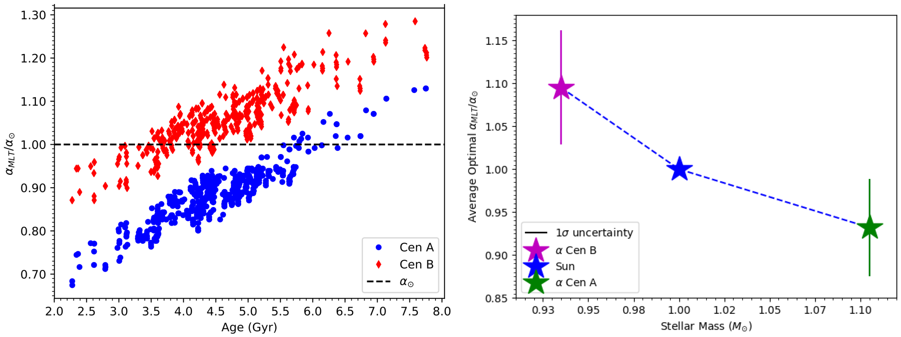
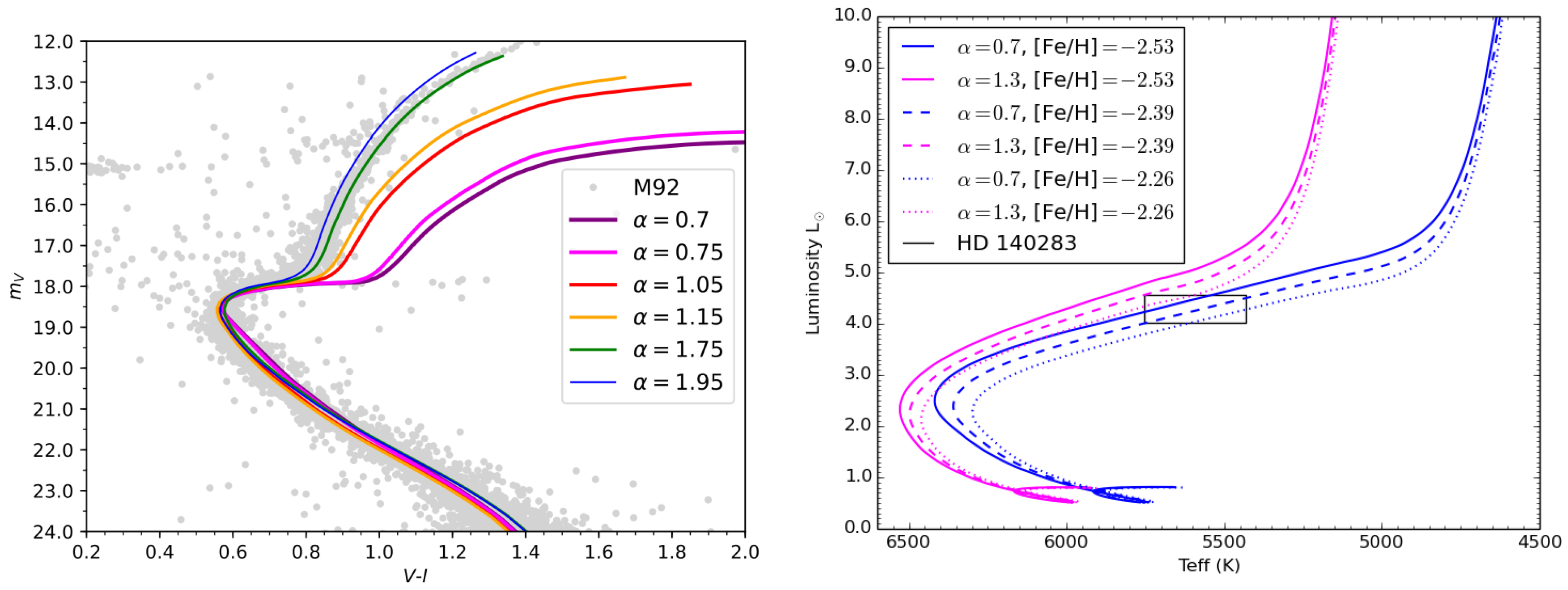
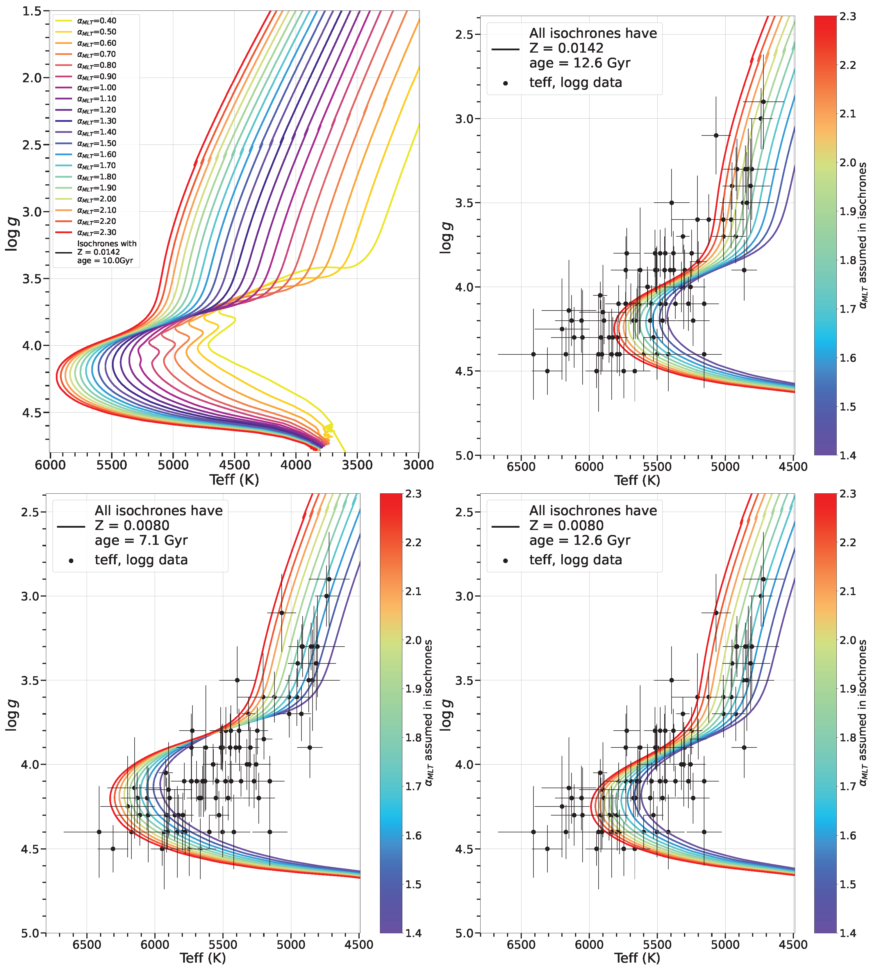
11. Non-Solar Calibrations

While the Sun is our best source of high-precision observational constraints, it is not an appropriate proxy for all stars. For the same reason, it is equally inappropriate to adopt the solar-calibrated mixing length ad hoc in any given stellar model. Until recently, however, there has simply not been an empirically motivated alternative.
Over the past few years, the identification of a handful of other stars with an appropriate number of independent observational constraints has opened the door to empirically calibrating the mixing length to non-solar targets. Due in particular to the availability of dynamical masses and robust asteroseismic information, the most reliable non-solar mixing length calibrations have been performed for Alpha Centauri A and B (Guenther and Demarque [118], Nsamba et al. [119], and Joyce and Chaboyer [86]). The left panel of Figure 6 is a reproduction from Joyce and Chaboyer [86], who found that, independent of other modeling choices, the optimal mixing length for α Cen B was always larger than the optimal mixing length for α Cen A in two-component models of the system, and that, in the majority of cases, the solar-calibrated value fell between them.
Less definitive but equally compelling work has been done on non-solar mixing length calibrations to very metal-poor stars, including the work of [83] on subgiant HD 140283, whose radius is known interferometrically. The need for sub-solar α M L T to reproduce the well-constrained temperature and luminosity of this star was later corroborated by Joyce and Chaboyer [85], who also found that sub-solar α MLT was necessary to fit stars of similar metal-poorness ([Fe/H]∼−2.4), regardless of evolutionary phase.
The probable dependence of α MLT on metallicity has been explored by numerous observers and 1D modellers in the past decade, including Tayar et al. [84], Viani et al. [87], Bonaca et al. [82], Song et al. [114], Nsamba et al. [119], and Joyce and Chaboyer [85]. Likewise, experts in 3D radiative hydrodynamics have argued, based on simulations of convection in the surface layers of stars, that the mixing length should depend on composition as well as surface gravity (e.g., Trampedach et al. [73], Magic et al. [74], Freytag et al. [120]); however, the relationship between α MLT and mass remains more elusive. Notably, Kervella et al. [121] found that models of the 61 Cygni binary system ( M = 0.7 and 0.6 M ; Z Z ) required a sub-solar mixing length, and argued that sub-solar values should be used for lower-mass stars in general. A decade later, Joyce and Chaboyer [86] noted a possible trend between α MLT and mass, as shown in the left panel of Figure 6.

12. Scientific Applications of Changing the Mixing Length

12.1. Implications for Age Measurements

There are two major ways in which changes to the mixing length can dramatically impact the estimation of stellar ages, which are used for a broad range of astrophysical purposes, from identifying the evolution of planetary systems to the enrichment and merger histories of galaxies. The first is directly: changing the mixing length changes the temperature structure, which changes the nuclear burning rates, which changes the lifetime of the star. Generally, increasing the mixing length decreases the main sequence lifetime, while decreasing the mixing length will increase the main sequence lifetime; however, this can become more complex, depending on how the model is calibrated. In a solar-calibrated model, for example, increasing the mixing length requires a decrease in helium to match the solar temperature at the solar age, which will then tend to increase the main sequence lifetime back towards or even above its base length.
The second way in which changing the mixing length can impact the inferred ages is less direct. As the models and their corresponding isochrones shift in temperature, the inferred age, given a set of observed parameters, will also shift. As a concrete example, one can imagine a red giant star observed by Gaia, whose luminosity can be inferred from its parallax, and whose temperature and metallicity can be inferred from photometry and spectroscopy. With those parameters, one has sufficient information to fit its age using a model; however, if the model uses a solar mixing length for all stars, rather than a metallicity-dependent one, we can expect the inferred mass of the star to shift by as much as 0.2 M (∼50 K) at [Fe/H] of ±0.5, even if the solar-metallicity models are properly calibrated (Tayar et al. [84]). That shift in mass would represent a change in the inferred age of several gigayears, even as large as a factor of two in some cases. Since the shift can be metallicity-dependent, it would then change the inferred age–metallicity relation of the galaxy, and fundamentally alter any inferences of its merger and enrichment history.
The right panel of Figure 7 demonstrates the degeneracy between metallicity and α MLT , using DSEP stellar tracks. The box represents brightness and temperature constraints for metal-poor subdwarf HD 140283, and the three different [Fe/H] assumptions in the tracks correspond to the minimum, maximum, and median values of the star’s measured metallicity (Creevey et al. [83]). This serves as an important indication that, even with excellent precision on HD 140283’s metallicity, it is not possible to determine, based on this information alone, whether α MLT = 1.3 or α MLT = 0.7 provides a better fit. At the same location in luminosity–temperature space, the α MLT = 0.7 track would provide an age estimate of order 1–2 Gyr younger than the age suggested by the α MLT = 1.3 curve.
Isochrones are the models most commonly used for age determinations, especially for stellar populations. Figure 7 shows a set of DSEP isochrones generated with various mixing lengths (colored curves) overlaid on HST photometry of the metal-poor globular cluster M92 (gray points). We note, in particular, the sensitivity of the subgiant and red giant portions of the isochrones to the choice of α MLT , likewise demonstrated in the MESA-based isochrones of Figure 5. The figure suggests that α MLT = 1.75 provides the best match to the data, which corresponds to a value ∼20% below the solar calibration ( α MLT , , DSEP = 1.9258 ); however, we are once again presented with the problem that the effects of changing α MLT are difficult to disentangle from the effects of changing the underlying composition assumptions of the isochrones—even more so than in the simpler (lower-dimensional) case of stellar tracks. As sharply demonstrated by the results of Joyce et al. [4], we must also reckon with the issue that the ages of isochrones are themselves degenerate with metallicity and α MLT , and the uncertainties in isochrone-based age determinations that do not account for this can be underestimated by a factor of two.
The upper left panel of Figure 8 shows the same models presented in Figure 5, but in the log g T eff plane instead. The remaining three panels show a subset of the tracks for which the mixing length assumption is varied between “reasonable extremes” for stars with masses between roughly 0.8 and 1.0 M , and metallicities, from slightly super-solar to values as low as [Fe/H] = 2.0 . The tracks in these panels sweep α MLT = 1.4 2.3 , corresponding to values calibrated for similar stars in the literature (e.g., Creevey et al. [83], Tayar et al. [84], Joyce and Chaboyer [85,86], Viani et al. [87], Tang and Joyce [122]). The black points show a sample of 91 micro-lensed subdwarfs with spectroscopic parameters determined by Bensby et al. [123]. The data serve to demonstrate that a physically motivated degree of variation in α MLT produces a shift in effective temperature that is at least comparable to the observational uncertainties on effective temperature; nor is the shift in log g negligible. The upper right and the two lower panels show that the spread induced by variation in α MLT is present in roughly equal measure for isochrones with ages of 12.6 Gyr and 7.1 Gyr, as well as for compositions near solar (Z = 0.0142) and [Fe/H]∼−0.3 (Z = 0.008), demonstrating that this effect is not restricted to one particular age or metallicity regime.

12.2. Implications for Nucleosynthesis

Changing the properties of convection by means of a change in the mixing length would also impact the expected nucleosynthetic processes, particularly for intermediate- and low-mass red giant and asymptotic giant branch stars. Such models also generally assume some sort of mixing length parameter, often a solar calibrated value (see, e.g., Lugaro et al. [124], Karakas and Lattanzio [125]). Increasing the mixing length parameter would increase the expected horizontal branch temperature, which then impacts the structure, lifetime, and mixing of AGB and super-AGB stars significantly. It has been argued that such changes can alter the predicted yields of some elements by as much as a factor of 3 (Doherty et al. [126]). It has also been found that using a different parameterization for convection, e.g., full-spectrum turbulence rather than the mixing length, can substantially change nucleosynthetic yields (Ventura et al. [127], Cinquegrana and Karakas [128]).

12.3. Implications for Stars in the Instability Strip

For some classes of pulsating stars, including γ Doradus and δ Scuti stars, the driving of pulsations is related to the interaction between the oscillations and convection, which depends on the properties, including size, of the convective zone (see (Houdek and Dupret [59]) for a thorough review of this topic). Changes in the mixing length will tend to change the size of the convective envelope at a given effective temperature, and thus will change the temperatures at which stars exhibit these oscillations. Specifically, decreasing the mixing length moves the instability strip towards lower temperature (Dupret et al. [129]). As large numbers of oscillating δ Scuti and γ Doradus stars have been detected by recent space missions (Van Reeth et al. [130], Murphy et al. [131], Antoci et al. [132], Aerts et al. [133]), it has now become possible to quantitatively compare the observed instability strips to predictions of models with different mixing lengths. Such comparisons seem to indicate that the observed instability strip is wider than that predicted by models, and one method for solving this would be to include models with a mass-dependent mixing length (Bowman and Kurtz [134]).
Work on the pulsation frequencies and amplitudes of classical pulsators, including Cepheids and RR Lyrae stars, has also indicated the dependence of the pulsations on the mixing length (e.g., Yecko et al. [135]), and the need for a more careful treatment of the interaction between convection and pulsation than standard mixing length theory permits (Stellingwerf [136]). The location of the red edge of the instability strip is particularly sensitive to the interactions between convection and pulsation (Baker and Gough [137]), (Stellingwerf [138], Bono et al. [139]), and analyses have indicated that the existence of double-mode pulsators may also relate to choices about convection (Kolláth et al. [140]—but see also Smolec and Moskalik [141]). More generally, reducing the mixing length tends to increase the minimum mass of stars that develop blue loops and, therefore, pass through the Cepheid instability phase. Similarly, changing the mixing length can shift the models such that additional mass loss is required before stars can populate the RR Lyrae instability strip. As even larger catalogs of carefully studied classical pulsators are being put together at a range of metallicities (e.g., Jurkovic et al. [142]), ongoing analysis is likely to place additional constraints on the necessary mixing lengths in these types of stars.

12.4. Implications for Galaxies

Studies of unresolved stellar populations, including star clusters and other galaxies, generally estimate the stellar populations present by comparing observed spectrophotometry to models of stellar evolution, combined to synthesize the expectation for a population (stellar population synthesis, e.g., (Maraston [143,144], Bruzual and Charlot [145], Conroy et al. [146])). As these models are based on stellar evolutionary tracks, they inherit the uncertainties of the underlying stellar models and their sensitivity to the choices of model physics, including the mixing length. As changes to the mixing length cause significant shifts in the temperature of the red giant branch, and the red giant branch contributes about a third of the bolometric flux in old populations (Maraston [143,144]), changes to the mixing length can substantially change the inferred ages of galactic populations (Goddard et al. [147]). As the mixing length may be related to stellar mass and metallicity, there are possible complexities that may be confusing our ability to infer the assembly and evolutionary history of the universe, a real issue in this time of rapidly improving data of galaxies from even earlier in time.

13. Successes of Mixing Length

The mixing length parameterization of convection has been astonishingly successful despite its simplicity. It has facilitated the creation of models of our own Sun, and of other stars, that have propelled our understanding of existing physics, have led to the discovery of entirely new physics, and have, in turn, given us the ability to describe the evolution of our galaxy and of the universe.

13.1. MLT and the Standard Solar Model

Models of stellar structure and evolution were used quite early on to comment on the possible energy generation mechanisms of stars (e.g., Cowling [148], Oke [149]), and, even in recent history, models of the Sun have been used as a stepping stone for discovering new facets of the universe. In the early 1990s, models of the Sun gave a predicted central temperature, fusion rate, and, therefore, neutrino flux that was inconsistent with measurements (e.g., Bahcall and Pinsonneault [150]). This helped to force discussion of other options for resolving the discrepancy, and eventually the neutrino oscillation model was accepted as a reasonable solution to the controversy (see accounts such as Perkins [151]).
More recently, absolute solar abundances have been an ongoing discussion. Spectroscopic analyses and helioseismic inversions based on solar models originally computed similar metal abundances for the Sun (Grevesse and Noels [152], Grevesse and Sauval [153]), but the incorporation of three-dimensional effects, and the impact of Non-Local Thermodynamic Equilibrium effects, into spectroscopic analyses seemed to argue for lower overall abundances (Asplund et al. [113]) that were incompatible with solar modeling (Basu and Antia [154]). New measurements of the solar rate of production of neutrinos from the CNO cycle seem to argue for a result more consistent with the results of solar modeling (Appel et al. [155]), as do some more recent estimates from spectroscopic analyses (Magg et al. [156]), and so, again, these may represent an instance where stellar models based on mixing length theory have encouraged the shift to a new standard paradigm, with implications for a wide range of analyses.

13.2. MLT and Asteroseismology

Models of stellar structure and evolution based on mixing length theory have also been sufficiently accurate to permit detailed asteroseismic analyses, allowing for the study of the detailed interior profiles of other stars, based on the exact frequencies and frequency ratios of their oscillation modes. While whole books can and have been written on the possibilities (Aerts et al. [157]) and methods (Basu and Chaplin [158]) of such analyses, we highlight here a few of the results that have enhanced the understanding of the physics of stellar interiors.
Comparisons of observations to stellar models created using mixing length theory have allowed for the identification of modes and mode patterns sensitive to the stellar interior, including sensitivity to the size of the convective core, and thus for mixing in overshoot regions (Van Reeth et al. [130], Pedersen [159], Deheuvels et al. [160], Constantino et al. [161]). They have also allowed for the identification of modes of mixed character, which probe the rotation profile of the interior of the star (Beck et al. [162], Deheuvels et al. [163], Mosser et al. [164]), and have potentially identified stars that have undergone interactions (Rui and Fuller [165], Deheuvels et al. [166], Li et al. [167], Matteuzzi et al. [168], Tayar et al. [169]). Models have identified modes that are missing or altered (García et al. [170], Stello et al. [171]), and it has been argued that these can probe the internal magnetic field strength and structure (Fuller et al. [172], Bugnet et al. [173]). More generally, asteroseismic analyses combined with stellar models have allowed for the estimation of ages for large populations of stars (e.g., Pinsonneault et al. [174]), and these results have then been used to infer the evolutionary histories of our own (Silva Aguirre et al. [175]) and other (Chaplin et al. [176], Grunblatt et al. [177]) galaxies, as well as having served as training sets for much larger explorations (Ness et al. [178], Leung et al. [179]).

14. Observational Challenges of Mixing Length

Given the remarkable success of one-dimensional evolutionary models of stars and their utility for studies of everything from extrasolar planets to the populations of the earliest galaxies, one might question whether there is still a need to devote effort to discussions of the choice of α MLT . We argue that such conversations must continue. Large numbers of stars are now observationally characterized to levels of precision that show that our simple assumptions about the mixing length generate demonstrably incorrect models. This has been identified through the careful calibration of individual stars (Joyce and Chaboyer [86]), the use of populations of clusters (Joyce and Chaboyer [85], Brasseur et al. [180], Cohen et al. [181], Smiljanic et al. [182]), constraints on other populations of stars (Ness et al. [183]), asteroseismic analysis of dwarf and giant stars (Bonaca et al. [82], Tayar et al. [84], Viani et al. [87], Metcalfe et al. [184], Creevey et al. [185], Silva Aguirre et al. [186]), efforts in the M dwarf regime (Somers and Pinsonneault [108], Feiden and Chaboyer [109]), and work on the location of the instability strip (Bowman and Kurtz [134]), to name only a few examples.
The most interesting and challenging part of the MLT landscape is that these analyses do not all agree with each other. Although each argues for a change in the mixing length, to better match observations, these changes do not converge to a single different value or scaling relation. Perhaps there exists a relationship between the mixing length and variables, such as mass, metallicity, surface gravity, temperature, magnetic field, etc., that could match all of the observational constraints over all regimes; however, no such single solution has yet been shown to work. It could also be the case that these discrepancies are showing us that the current mixing length framework is ultimately insufficient for the modern observational data climate, and that there is a real need for a new paradigm.
Another open question concerns the inability of more sophisticated three-dimensional simulations to predict a mixing length that matches the requirements from the observations (see, e.g., Figure 9, reproduced from Tayar et al. [84]). The translation from a three-dimensional simulation to some estimate of a mixing length is not straightforward (Trampedach et al. [73], Magic et al. [74]), as there is no clear physical definition for such a parameter, so the lack of correspondence could be a translation issue rather than evidence of missing physical understanding. Three-dimensional simulations of convection also have their own challenges (Miesch [187]), as do observational calibrations to place stars on a fundamental scale (Tayar et al. [2]). Even so, the inability to predict the mixing length from well-known physical principles calls into question its long-term viability as a relevant model.

15. The Future of MLT

Having reviewed both the extraordinary successes and the substantial limitations of the mixing length theory of convection, we now speculate on what the future holds for MLT.
First and foremost, we expect the evolution of MLT to be driven observationally. As both data quality and data volume increase at unprecedented rates, the data will require models of a higher standard, to make sense of abundant, high-precision observational constraints from multiple sources, and to extend the interpretation of data to regimes where the data are not yet sufficient to constrain the model.
On the 5–10-year horizon, we can expect to see empirical calibrations of α MLT to an increasingly broad, globally representative sample of non-solar targets, and for these data-driven values to increasingly replace ad hoc use of the solar prescription. Carefully characterized targets with well-constrained masses, compositions, and radii will be assembled into a list of calibration targets used to determine the appropriate mixing length for an individual model grid; we expect these targets to come from a combination of eclipsing binary analysis, open cluster membership, and/or photometric, astrometric, spectroscopic, and asteroseismic data. Grids of models that span various physical assumptions will be generated, to estimate the appropriate mixing length for each star’s particular composition, temperature, and surface gravity. Arguments will be made about whether a single mixing length should then be used to fit all stars with mass X and/or metallicity Y, whether there is a scaling relation between α MLT and other stellar parameters that should be applied universally or in particular evolutionary phases/mass regimes, or whether models should be using a static mixing length, rather than one that changes over time, at all. Comparisons will be made to three-dimensional models to determine if they can be processed in such a way as to provide useful insight on the changes to the mixing length. Stellar evolution codes will be modified to accommodate such schemes, and, over time, we will learn which approaches are better.
We expect that this paradigm of iterative, data-informed revision and improvement will persist for a time, and then the data will once again improve. At that point, it will become clearer whether the calibrated mixing length framework is sufficient to predict the evolution, temperature, and ages of stars to an acceptable precision. When that happens, the researchers of the future may finally have to find an implementation of convection with greater physical fidelity, to use in stellar evolution calculations; alternatively, they may once again discover that the humble mixing length prescription once again requires only slight modifications to do a truly excellent job predicting the behavior and evolution of stars across the Hertzsprung–Russell diagram. In either case, researchers will be driven to make choices that preserve stellar models’ place as a fundamental pillar of astrophysics.

Author Contributions

Conceptualization, M.J. and J.T.; methodology, M.J. and J.T.; software, M.J. and J.T.; validation, M.J. and J.T.; formal analysis, M.J. and J.T.; investigation, M.J. and J.T.; resources, M.J. and J.T.; data curation, J.T.; writing—original draft preparation, M.J. and J.T.; writing—review and editing, M.J. and J.T.; visualization, M.J. and J.T.; supervision, M.J.; project administration, M.J.; funding acquisition, M.J. and J.T.. All authors have read and agreed to the published version of the manuscript.

Funding

M.J. gratefully acknowledges funding of MATISSE: Measuring Ages Through Isochrones, Seismology, and Stellar Evolution, awarded through the European Commission’s Widening Fellowship. This project received funding from the European Union’s Horizon 2020 research and innovation program. J.T. and M.J. acknowledge support from NASA grant 80NSSC22K0812. This series was conceived at the 2021 KITP program Probes of Transport in Stars, supported by NSF grant number NSF PHY-1748958.

Data Availability Statement

No new data were created or analyzed in this study. Data sharing is not applicable to this article.

Acknowledgments

The authors wish to thank László Molnár for sharing his expertise in classical stellar variability, and Giulia Cinquegrana for sharing her expertise in TP-AGB stars, both of which contributed to this manuscript. The authors also wish to thank John Bourke for revisions and discussion.

Conflicts of Interest

The authors declare no conflict of interest. The funders had no role in the design of the study; in the collection, analyses, or interpretation of data; in the writing of the manuscript; or in the decision to publish the results.

Notes

1
Meaning the one-dimensional distance element is taken to be the fractional radius d r , rather than the mass, d m .
2
For discussion of the difference between these criteria and where they are applicable, consider reading e.g., Gabriel et al. [49], Salaris and Cassisi [50], Anders et al. [51].
3
That is, where entropy is constant.
4
More precisely, it is the lack of an efficiency differential in the convective core that makes the choice of α MLT irrelevant in this regime.
5
The treatment of core convective boundaries is particularly important for determining whether massive stars will meet the M core criterion for death as a supernova.

References

  1. Choi, J.; Dotter, A.; Conroy, C.; Ting, Y.S. On the Red Giant Branch: Ambiguity in the Surface Boundary Condition Leads to ≈100 K Uncertainty in Model Effective Temperatures. Astrophys. J. 2018, 860, 131. [Google Scholar] [CrossRef] [Green Version]
  2. Tayar, J.; Claytor, Z.R.; Huber, D.; van Saders, J. A Guide to Realistic Uncertainties on the Fundamental Properties of Solar-type Exoplanet Host Stars. Astrophys. J. 2022, 927, 31. [Google Scholar] [CrossRef]
  3. Cinquegrana, G.C.; Joyce, M.; Karakas, A.I. Bridging the Gap between Intermediate and Massive Stars. I. Validation of MESA against the State-of-the-Art Monash Stellar Evolution Program for a 2M AGB Star. Astrophys. J. 2022, 939, 50. [Google Scholar] [CrossRef]
  4. Joyce, M.; Johnson, C.I.; Marchetti, T.; Rich, R.M.; Simion, I.; Bourke, J. The Ages of Galactic Bulge Stars with Realistic Uncertainties. arXiv 2022, arXiv:2205.07964. [Google Scholar] [CrossRef]
  5. Böhm-Vitense, E. Über die Wasserstoffkonvektionszone in Sternen verschiedener Effektivtemperaturen und Leuchtkräfte. Mit 5 Textabbildungen. Z. Astrophys. 1958, 46, 108. [Google Scholar]
  6. Ventura, P.; Zeppieri, A.; Mazzitelli, I.; D’Antona, F. Full spectrum of turbulence convective mixing: I. theoretical main sequences and turn-off for 0.6/∖15 M_∖odot. Astron. Astrophys. 1998, 334, 953–968. [Google Scholar]
  7. Ventura, P.; Di Criscienzo, M.; Carini, R.; D’Antona, F. Yields of AGB and SAGB models with chemistry of low- and high-metallicity globular clusters. Mon. Not. R. Astron. Soc. 2013, 431, 3642–3653. [Google Scholar] [CrossRef]
  8. Pietrinferni, A.; Cassisi, S.; Salaris, M.; Castelli, F. A large stellar evolution database for population synthesis studies. I. Scaled solar models and isochrones. Astrophys. J. 2004, 612, 168. [Google Scholar] [CrossRef]
  9. Eggleton, P.P. The evolution of low mass stars. Mon. Not. R. Astron. Soc. 1971, 151, 351–364. [Google Scholar] [CrossRef] [Green Version]
  10. Morel, P.; Lebreton, Y. CESAM: A free code for stellar evolution calculations. Astrophys. Space Sci. 2008, 316, 61–73. [Google Scholar] [CrossRef]
  11. Dotter, A.; Chaboyer, B.; Jevremović, D.; Kostov, V.; Baron, E.; Ferguson, J.W. The Dartmouth Stellar Evolution Database. Astrophys. J. Suppl. Ser. 2008, 178, 89–101. [Google Scholar] [CrossRef] [Green Version]
  12. Weiss, A.; Schlattl, H. GARSTEC—the Garching Stellar Evolution Code. Astrophys. Space Sci. 2008, 316, 99–106. [Google Scholar] [CrossRef] [Green Version]
  13. Charbonnel, C.; Meynet, G.; Maeder, A.; Schaerer, D. Grids of stellar models. VI. Horizontal branch and early asymptotic giant branch for low mass stars (Z = 0.020, 0.001). Astron. Astrophys. Suppl. Ser. 1996, 115, 339. [Google Scholar]
  14. Jermyn, A.S.; Bauer, E.B.; Schwab, J.; Farmer, R.; Ball, W.H.; Bellinger, E.P.; Dotter, A.; Joyce, M.; Marchant, P.; Mombarg, J.S.G.; et al. Modules for Experiments in Stellar Astrophysics (MESA): Time-Dependent Convection, Energy Conservation, Automatic Differentiation, and Infrastructure. arXiv 2022, arXiv:2208.03651. [Google Scholar] [CrossRef]
  15. Paxton, B.; Smolec, R.; Schwab, J.; Gautschy, A.; Bildsten, L.; Cantiello, M.; Dotter, A.; Farmer, R.; Goldberg, J.A.; Jermyn, A.S.; et al. Modules for experiments in stellar astrophysics (MESA): Pulsating variable stars, rotation, convective boundaries, and energy conservation. Astrophys. J. Suppl. Ser. 2019, 243, 10. [Google Scholar] [CrossRef]
  16. Paxton, B.; Schwab, J.; Bauer, E.B.; Bildsten, L.; Blinnikov, S.; Duffell, P.; Farmer, R.; Goldberg, J.A.; Marchant, P.; Sorokina, E.; et al. Modules for Experiments in Stellar Astrophysics (MESA): Convective Boundaries, Element Diffusion, and Massive Star Explosions. Astrophys. J. Suppl. Ser. 2018, 234, 34. [Google Scholar] [CrossRef]
  17. Paxton, B.; Marchant, P.; Schwab, J.; Bauer, E.B.; Bildsten, L.; Cantiello, M.; Dessart, L.; Farmer, R.; Hu, H.; Langer, N.; et al. Modules for experiments in stellar astrophysics (MESA): Binaries, pulsations, and explosions. Astrophys. J. Suppl. Ser. 2015, 220, 15. [Google Scholar] [CrossRef]
  18. Paxton, B.; Cantiello, M.; Arras, P.; Bildsten, L.; Brown, E.F.; Dotter, A.; Mankovich, C.; Montgomery, M.; Stello, D.; Timmes, F.; et al. Modules for experiments in stellar astrophysics (MESA): Planets, oscillations, rotation, and massive stars. Astrophys. J. Suppl. Ser. 2013, 208, 4. [Google Scholar] [CrossRef] [Green Version]
  19. Paxton, B.; Bildsten, L.; Dotter, A.; Herwig, F.; Lesaffre, P.; Timmes, F. Modules for experiments in stellar astrophysics (MESA). Astrophys. J. Suppl. Ser. 2010, 192, 3. [Google Scholar] [CrossRef]
  20. Lattanzio, J.C. The Evolution of Initially Inhomogeneous Stars and Low Mass AGB Stars. Ph.D. Thesis, Monash University, Clayton, Australia, 1984. [Google Scholar]
  21. Lattanzio, J.C. The asymptotic giant branch evolution of 1.0-3.0 solar mass stars as a function of mass and composition. Astrophys. J. 1986, 311, 708–730. [Google Scholar] [CrossRef]
  22. Frost, C.; Lattanzio, J. On the numerical treatment and dependence of the third dredge-up phenomenon. Astrophys. J. 1996, 473, 383. [Google Scholar] [CrossRef] [Green Version]
  23. Karakas, A.; Lattanzio, J.C. Stellar models and yields of asymptotic giant branch stars. Pub. Astron. Soc. Aus. 2007, 24, 103–117. [Google Scholar] [CrossRef] [Green Version]
  24. Bressan, A.; Marigo, P.; Girardi, L.; Salasnich, B.; Dal Cero, C.; Rubele, S.; Nanni, A. PARSEC: Stellar tracks and isochrones with the PAdova and TRieste Stellar Evolution Code. Mon. Not. R. Astron. Soc. 2012, 427, 127–145. [Google Scholar] [CrossRef] [Green Version]
  25. Demarque, P.; Guenther, D.; Li, L.; Mazumdar, A.; Straka, C. YREC: The Yale rotating stellar evolution code. Astrophys. Space Sci. 2008, 316, 31–41. [Google Scholar] [CrossRef] [Green Version]
  26. Canuto, V.M.; Mazzitelli, I. Stellar Turbulent Convection: A New Model and Applications. Astrophys. J. 1991, 370, 295–311. [Google Scholar] [CrossRef]
  27. Canuto, V.; Goldman, I.; Mazzitelli, I. Stellar turbulent convection: A self-consistent model. Astrophys. J. 1996, 473, 550. [Google Scholar] [CrossRef] [Green Version]
  28. Gaia Collaboration; Brown, A.G.A.; Vallenari, A.; Prusti, T.; de Bruijne, J.H.J.; Babusiaux, C.; Biermann, M.; Creevey, O.L.; Evans, D.W.; Eyer, L.; et al. Gaia Early Data Release 3. Summary of the contents and survey properties. Astron. Astrophys. 2021, 649, A1. [Google Scholar] [CrossRef]
  29. Ricker, G.R.; Winn, J.N.; Vanderspek, R.; Latham, D.W.; Bakos, G.Á.; Bean, J.L.; Berta-Thompson, Z.K.; Brown, T.M.; Buchhave, L.; Butler, N.R.; et al. Transiting Exoplanet Survey Satellite (TESS). J. Astron. Telesc. Instruments Syst. 2015, 1, 014003. [Google Scholar] [CrossRef] [Green Version]
  30. Borucki, W.J.; Koch, D.; Basri, G.; Batalha, N.; Brown, T.; Caldwell, D.; Caldwell, J.; Christensen-Dalsgaard, J.; Cochran, W.D.; DeVore, E.; et al. Kepler Planet-Detection Mission: Introduction and First Results. Science 2010, 327, 977. [Google Scholar] [CrossRef] [Green Version]
  31. LSST Science Collaboration; Marshall, P.; Anguita, T.; Bianco, F.B.; Bellm, E.C.; Brandt, N.; Clarkson, W.; Connolly, A.; Gawiser, E.; Ivezic, Z.; et al. Science-Driven Optimization of the LSST Observing Strategy. arXiv 2017, arXiv:1708.04058. [Google Scholar]
  32. Majewski, S.R.; Schiavon, R.P.; Frinchaboy, P.M.; Allende Prieto, C.; Barkhouser, R.; Bizyaev, D.; Blank, B.; Brunner, S.; Burton, A.; Carrera, R.; et al. The Apache Point Observatory Galactic Evolution Experiment (APOGEE). Astron. J. 2017, 154, 94. [Google Scholar] [CrossRef]
  33. Cui, X.Q.; Zhao, Y.H.; Chu, Y.Q.; Li, G.P.; Li, Q.; Zhang, L.P.; Su, H.J.; Yao, Z.Q.; Wang, Y.N.; Xing, X.Z.; et al. The Large Sky Area Multi-Object Fiber Spectroscopic Telescope (LAMOST). Res. Astron. Astrophys. 2012, 12, 1197–1242. [Google Scholar] [CrossRef]
  34. Buder, S.; Sharma, S.; Kos, J.; Amarsi, A.M.; Nordlander, T.; Lind, K.; Martell, S.L.; Asplund, M.; Bland-Hawthorn, J.; Casey, A.R.; et al. The GALAH+ survey: Third data release. Mon. Not. R. Astron. Soc. 2021, 506, 150–201. [Google Scholar] [CrossRef]
  35. Prandtl, L. Bericht über Untersuchungen zur ausgebildeten Turbulenz. Z. Angew. Math. Mech. 1925, 136. [Google Scholar] [CrossRef]
  36. Vitense, E. Die wasserstoffkonvektionszone der sonne. Mit 11 textabbildungen. Z. Astrophys. 1953, 32, 135. [Google Scholar]
  37. Henyey, L.; Vardya, M.; Bodenheimer, P. Studies in stellar evolution. III. The calculation of model envelopes. Astrophys. J. 1965, 142, 841. [Google Scholar] [CrossRef]
  38. Cox, J.; Giuli, R. Principles of Stellar Structure; Gordon and Breach: New York, NY, USA, 1968. [Google Scholar]
  39. Bohm, K.H.; Cassinelli, J. Convective Envelopes and Acoustic Noise Generation in White Dwarfs. Astron. Astrophys. 1971, 12, 21. [Google Scholar]
  40. Mihalas, D.; Auer, L.H.; Mihalas, B.R. Two-dimensional radiative transfer. I. Planar geometry. Astrophys. J. 1978, 220, 1001–1023. [Google Scholar] [CrossRef]
  41. Mihalas, D. Stellar Atmospheres; WH Freeman: San Francisco, CA, USA, 1978. [Google Scholar]
  42. Kurucz, R.L. Model atmospheres for G, F, A, B, and O stars. Astrophys. J. Suppl. Ser. 1979, 40, 1–340. [Google Scholar] [CrossRef]
  43. Basu, S.; Antia, H.M.; Narasimha, D. Helioseismic measurement of the extent of overshoot below the solar convection zone. Mon. Not. R. Astron. Soc. 1994, 267, 209. [Google Scholar] [CrossRef] [Green Version]
  44. Basu, S.; Pinsonneault, M.H.; Bahcall, J.N. How Much Do Helioseismological Inferences Depend on the Assumed Reference Model? Astrophys. J. 2000, 529, 1084–1100. [Google Scholar] [CrossRef] [Green Version]
  45. Demarque, P.; Guenther, D.B.; Kim, Y.C. The Run of Superadiabaticity in Stellar Convection Zones. I. The Sun. Astrophys. J. 1997, 474, 790–797. [Google Scholar] [CrossRef] [Green Version]
  46. Demarque, P.; Guenther, D.B.; Kim, Y.C. The Run of Superadiabaticity in Stellar Convection Zones. II. Effect of Photospheric Convection on Solar p-Mode Frequencies. Astrophys. J. 1999, 517, 510–515. [Google Scholar] [CrossRef] [Green Version]
  47. Schwarzschild, M. Structure and Evolution of the Stars; Princeton University Press: Princeton, NJ, USA, 1958. [Google Scholar]
  48. Ledoux, P. Stellar Models with Convection and with Discontinuity of the Mean Molecular Weight. Astrophys. J. 1947, 105, 305. [Google Scholar] [CrossRef]
  49. Gabriel, M.; Noels, A.; Montalbán, J.; Miglio, A. Proper Use of Schwarzschild Ledoux Criteria in Stellar Evolution Computations. Astron. Astrophys. 2014, 569, A63. [Google Scholar] [CrossRef] [Green Version]
  50. Salaris, M.; Cassisi, S. Chemical element transport in stellar evolution models. R. Soc. Open Sci. 2017, 4, 170192. [Google Scholar] [CrossRef] [Green Version]
  51. Anders, E.H.; Jermyn, A.S.; Lecoanet, D.; Fraser, A.E.; Cresswell, I.G.; Joyce, M.; Fuentes, J. Schwarzschild and Ledoux are equivalent on evolutionary timescales. Astrophys. J. Lett. 2022, 928, L10. [Google Scholar] [CrossRef]
  52. Kippenhahn, R.; Weigert, A. Stellar Structure and Evolution; Springer: Berlin/Heidelberg, Germany, 1994. [Google Scholar]
  53. Stein, R.F.; Nordlund, A. Topology of convection beneath the solar surface. Astrophys. J. 1989, 342, L95–L98. [Google Scholar] [CrossRef]
  54. Salaris, M.; Cassisi, S. Evolution of Stars and Stellar Populations; Wiley: Hoboken, NJ, USA, 2006. [Google Scholar]
  55. Henyey, L.G.; Forbes, J.E.; Gould, N.L. A New Method of Automatic Computation of Stellar Evolution. Astrophys. J. 1964, 139, 306. [Google Scholar] [CrossRef]
  56. Kurucz, R.L. Progress on model atmospheres and line data. In Proceedings of the IAU Symposium, Kyoto, Japan, 18–22 August 1997; Volume 189, pp. 217–226. [Google Scholar]
  57. Unno, W. Stellar Radial Pulsation Coupled with the Convection. Publ. Astron. Soc. Jpn. 1967, 19, 140. [Google Scholar]
  58. Gough, D.O.; Ostriker, J.P.; Stobie, R.S. On the Periods of Pulsating Stars. Astrophys. J. 1965, 142, 1649–1652. [Google Scholar] [CrossRef]
  59. Houdek, G.; Dupret, M.A. Interaction Between Convection and Pulsation. Living Rev. Sol. Phys. 2015, 12, 8. [Google Scholar] [CrossRef]
  60. Kuhfuss, R. A model for time-dependent turbulent convection. Astron. Astrophys. 1986, 160, 116–120. [Google Scholar]
  61. Gough, D.O. Mixing-length theory for pulsating stars. Astrophys. J. 1977, 214, 196–213. [Google Scholar] [CrossRef]
  62. Renzini, A. Some embarrassments in current treatments of convective overshooting. Astron. Astrophys. 1987, 188, 49–54. [Google Scholar]
  63. Grossman, S.A.; Narayan, R. A Theory of Nonlocal Mixing-Length Convection. II. Generalized Smoothed Particle Hydrodynamics Simulations. Astrophys. J. Suppl. Ser. 1993, 89, 361. [Google Scholar] [CrossRef]
  64. Eggleton, P.P. Towards consistency in simple prescriptions for stellar convection. Mon. Not. R. Astron. Soc. 1983, 204, 449–461. [Google Scholar] [CrossRef] [Green Version]
  65. Xiong, D.R. The evolution of massive stars using a non-local theory of convection. Astron. Astrophys. 1986, 167, 239–246. [Google Scholar]
  66. Xiong, D.R. Radiation-hydrodynamic equations for stellar oscillations. Astron. Astrophys. 1989, 209, 126–134. [Google Scholar]
  67. Xiong, D.R. Numerical simulations of nonlocal convection. Astron. Astrophys. 1989, 213, 176–182. [Google Scholar]
  68. Grossman, S.A. A theory of non-local mixing-length convection-III. Comparing theory and numerical experiment. Mon. Not. R. Astron. Soc. 1996, 279, 305–336. [Google Scholar] [CrossRef] [Green Version]
  69. Ireland, L.G.; Browning, M.K. The Radius and Entropy of a Magnetized, Rotating, Fully Convective Star: Analysis with Depth-dependent Mixing Length Theories. Astrophys. J. 2018, 856, 132. [Google Scholar] [CrossRef] [Green Version]
  70. Marcus, P.S.; Press, W.H.; Teukolsky, S.A. Multiscale model equations for turbulent convection and convective overshoot. Astrophys. J. 1983, 267, 795–821. [Google Scholar] [CrossRef]
  71. Arnett, W.D.; Meakin, C.; Viallet, M.; Campbell, S.W.; Lattanzio, J.C.; Mocák, M. Beyond Mixing-length Theory: A Step Toward 321D. Astrophys. J. 2015, 809, 30. [Google Scholar] [CrossRef] [Green Version]
  72. Arnett, W.D.; Hirschi, R.; Campbell, S.W.; Mocák, M.; Georgy, C.; Meakin, C.; Cristini, A.; Scott, L.J.A.; Kaiser, E.A.; Viallet, M. 3D Simulations and MLT: II. Onsager’s Ideal Turbulence. arXiv 2018, arXiv:1810.04659. [Google Scholar] [CrossRef]
  73. Trampedach, R.; Stein, R.F.; Christensen-Dalsgaard, J.; Nordlund, Å.; Asplund, M. Improvements to stellar structure models, based on a grid of 3D convection simulations—II. Calibrating the mixing-length formulation. Mon. Not. R. Astron. Soc. 2014, 445, 4366–4384. [Google Scholar] [CrossRef]
  74. Magic, Z.; Weiss, A.; Asplund, M. The Stagger-grid: A grid of 3D stellar atmosphere models. III. The relation to mixing length convection theory. Astron. Astrophys. 2015, 573, A89. [Google Scholar] [CrossRef]
  75. Sonoi, T.; Ludwig, H.G.; Dupret, M.A.; Montalban, J.; Belkacem, K.; Caffau, E. Calibration of the mixing length of the MLT and FST models using 3D hydrodynamical models. In PHysics of Oscillating STars, Proceedings of the PHOST (PHysics of Oscillating STars) Symposium Hosted by the Oceanographic Observatory in Banyuls-sur-mer (France) from 2–7 September 2018; This Conference Honours the Life Work of Professor Hiromoto Shibahashi; Tokyo University: Tokyo, Japan, 2018; p. 27. [Google Scholar] [CrossRef]
  76. Tanner, J.D.; Basu, S.; Demarque, P. The Effect of Metallicity-dependent T-τ Relations on Calibrated Stellar Models. Astrophys. J. 2014, 785, L13. [Google Scholar] [CrossRef] [Green Version]
  77. Salaris, M.; Cassisi, S. Stellar models with mixing length and T(τ) relations calibrated on 3D convection simulations. Astron. Astrophys. 2015, 577, A60. [Google Scholar] [CrossRef] [Green Version]
  78. Mosumgaard, J.R.; Ball, W.H.; Silva Aguirre, V.; Weiss, A.; Christensen-Dalsgaard, J. Stellar models with calibrated convection and temperature stratification from 3D hydrodynamics simulations. Mon. Not. R. Astron. Soc. 2018, 478, 5650–5659. [Google Scholar] [CrossRef]
  79. Zhou, Y.; Asplund, M.; Collet, R.; Joyce, M. Convective excitation and damping of solar-like oscillations. Mon. Not. R. Astron. Soc. 2020, 495, 4904–4923. [Google Scholar] [CrossRef]
  80. Spada, F.; Demarque, P. Testing the entropy calibration of the radii of cool stars: Models of α Centauri A and B. Mon. Not. R. Astron. Soc. 2019, 489, 4712–4720. [Google Scholar] [CrossRef]
  81. Spada, F.; Demarque, P.; Kupka, F. Stellar evolution models with entropy-calibrated mixing-length parameter: Application to red giants. Mon. Not. R. Astron. Soc. 2021, 504, 3128–3138. [Google Scholar] [CrossRef]
  82. Bonaca, A.; Tanner, J.D.; Basu, S.; Chaplin, W.J.; Metcalfe, T.S.; Monteiro, M.J.P.F.G.; Ballot, J.; Bedding, T.R.; Bonanno, A.; Broomhall, A.M.; et al. Calibrating Convective Properties of Solar-like Stars in the Kepler Field of View. Astrophys. J. 2012, 755, L12. [Google Scholar] [CrossRef] [Green Version]
  83. Creevey, O.L.; Thévenin, F.; Berio, P.; Heiter, U.; von Braun, K.; Mourard, D.; Bigot, L.; Boyajian, T.S.; Kervella, P.; Morel, P.; et al. Benchmark stars for Gaia Fundamental properties of the Population II star HD 140283 from interferometric, spectroscopic, and photometric data. Astron. Astrophys. 2015, 575, A26. [Google Scholar] [CrossRef] [Green Version]
  84. Tayar, J.; Somers, G.; Pinsonneault, M.H.; Stello, D.; Mints, A.; Johnson, J.A.; Zamora, O.; García-Hernández, D.A.; Maraston, C.; Serenelli, A.; et al. The Correlation between Mixing Length and Metallicity on the Giant Branch: Implications for Ages in the Gaia Era. Astrophys. J. 2017, 840, 17. [Google Scholar] [CrossRef] [Green Version]
  85. Joyce, M.; Chaboyer, B. Not All Stars Are the Sun: Empirical Calibration of the Mixing Length for Metal-poor Stars Using One-dimensional Stellar Evolution Models. Astrophys. J. 2018, 856, 10. [Google Scholar] [CrossRef]
  86. Joyce, M.; Chaboyer, B. Classically and Asteroseismically Constrained 1D Stellar Evolution Models of α Centauri A and B Using Empirical Mixing Length Calibrations. Astrophys. J. 2018, 864, 99. [Google Scholar] [CrossRef] [Green Version]
  87. Viani, L.S.; Basu, S.; Joel Ong J., M.; Bonaca, A.; Chaplin, W.J. Investigating the Metallicity-Mixing-length Relation. Astrophys. J. 2018, 858, 28. [Google Scholar] [CrossRef] [Green Version]
  88. Valle, G.; Dell’Omodarme, M.; Prada Moroni, P.G.; Degl’Innocenti, S. Mixing-length calibration from field stars. An investigation on statistical errors, systematic biases, and spurious metallicity trends. Astron. Astrophys. 2019, 623, A59. [Google Scholar] [CrossRef] [Green Version]
  89. Krishna Swamy, K.S. Profiles of Strong Lines in K-Dwarfs. Astrophys. J. 1966, 145, 174–195. [Google Scholar] [CrossRef]
  90. Ball, W.H. A Novel Analytic Atmospheric T(τ) Relation for Stellar Models. Res. Notes Am. Astron. Soc. 2021, 5, 7. [Google Scholar] [CrossRef]
  91. Castelli, F.; Kurucz, R.L. New Grids of ATLAS9 Model Atmospheres. arXiv 2004, arXiv:astro-ph/0405087. [Google Scholar]
  92. Hauschildt, P.H.; Allard, F.; Baron, E. The NextGen Model Atmosphere Grid for 3000 ≤ Teff ≤ 10,000 K. Astrophys. J. 1999, 512, 377–385. [Google Scholar] [CrossRef] [Green Version]
  93. Gustafsson, B. Is the Sun unique as a star—and if so, why? Phys. Scr. Vol. T 2008, 130, 014036. [Google Scholar] [CrossRef]
  94. Song, N.; Alexeeva, S.; Sitnova, T.; Wang, L.; Grupp, F.; Zhao, G. Impact of the convective mixing-length parameter α on stellar metallicity. Astron. Astrophys. 2020, 635, A176. [Google Scholar] [CrossRef] [Green Version]
  95. Mosumgaard, J.R.; Jørgensen, A.C.S.; Weiss, A.; Silva Aguirre, V.; Christensen-Dalsgaard, J. Coupling 1D stellar evolution with 3D-hydrodynamical simulations on-the-fly II: Stellar evolution and asteroseismic applications. Mon. Not. R. Astron. Soc. 2020, 491, 1160–1173. [Google Scholar] [CrossRef] [Green Version]
  96. Pedersen, M.G.; Aerts, C.; Pápics, P.I.; Michielsen, M.; Gebruers, S.; Rogers, T.M.; Molenberghs, G.; Burssens, S.; Garcia, S.; Bowman, D.M. Internal mixing of rotating stars inferred from dipole gravity modes. Nat. Astron. 2021, 5, 715–722. [Google Scholar] [CrossRef]
  97. Karakas, A.I.; Cinquegrana, G.; Joyce, M. The most metal-rich asymptotic giant branch stars. Mon. Not. R. Astron. Soc. 2022, 509, 4430–4447. [Google Scholar] [CrossRef]
  98. Mirouh, G.M.; Garaud, P.; Stellmach, S.; Traxler, A.L.; Wood, T.S. A New Model for Mixing by Double-diffusive Convection (Semi-convection). I. The Conditions for Layer Formation. Astrophys. J. 2012, 750, 61. [Google Scholar] [CrossRef]
  99. Pietrinferni, A.; Cassisi, S.; Salaris, M.; Percival, S.; Ferguson, J.W. A Large Stellar Evolution Database for Population Synthesis Studies. V. Stellar Models and Isochrones with CNONa Abundance Anticorrelations. Astrophys. J. 2009, 697, 275–282. [Google Scholar] [CrossRef]
  100. Beom, M.; Na, C.; Ferguson, J.W.; Kim, Y.C. The Effects of Individual Metal Contents on Isochrones for C, N, O, Na, Mg, Al, Si, and Fe. Astrophys. J. 2016, 826, 155. [Google Scholar] [CrossRef] [Green Version]
  101. van Saders, J.L.; Pinsonneault, M.H. The Sensitivity of Convection Zone Depth to Stellar Abundances: An Absolute Stellar Abundance Scale from Asteroseismology. Astrophys. J. 2012, 746, 16. [Google Scholar] [CrossRef] [Green Version]
  102. Cinquegrana, G.C.; Joyce, M. Solar Calibration of the Convective Mixing Length for Use with the ÆSOPUS Opacities in MESA. Res. Notes AAS 2022, 6, 77. [Google Scholar] [CrossRef]
  103. Roudier, T.; Ballot, J.; Malherbe, J.M.; Chane-Yook, M. Texture of average solar photospheric flows and the donut-like pattern. arXiv 2023, arXiv:2301.07988. [Google Scholar] [CrossRef]
  104. Gosnell, N.M.; Gully-Santiago, M.A.; Leiner, E.M.; Tofflemire, B.M. Observationally Constraining the Starspot Properties of Magnetically Active M67 Sub-subgiant S1063. Astrophys. J. 2022, 925, 5. [Google Scholar] [CrossRef]
  105. Libby-Roberts, J.E.; Schutte, M.; Hebb, L.; Kanodia, S.; Canas, C.; Stefansson, G.; Lin, A.S.J.; Mahadevan, S.; Parts, W.; Powers, L.; et al. An In-Depth Look at TOI-3884b: A Super-Neptune Transiting a M4 Dwarf with Persistent Star Spot Crossings. arXiv 2023, arXiv:2302.04757. [Google Scholar] [CrossRef]
  106. Somers, G.; Pinsonneault, M.H. Older and Colder: The Impact of Starspots on Pre-main-sequence Stellar Evolution. Astrophys. J. 2015, 807, 174. [Google Scholar] [CrossRef] [Green Version]
  107. Chabrier, G.; Gallardo, J.; Baraffe, I. Evolution of low-mass star and brown dwarf eclipsing binaries. Astron. Astrophys. 2007, 472, L17–L20. [Google Scholar] [CrossRef] [Green Version]
  108. Somers, G.; Pinsonneault, M.H. A Tale of Two Anomalies: Depletion, Dispersion, and the Connection between the Stellar Lithium Spread and Inflated Radii on the Pre-main Sequence. Astrophys. J. 2014, 790, 72. [Google Scholar] [CrossRef] [Green Version]
  109. Feiden, G.A.; Chaboyer, B. Self-consistent Magnetic Stellar Evolution Models of the Detached, Solar-type Eclipsing Binary EF Aquarii. Astrophys. J. 2012, 761, 30. [Google Scholar] [CrossRef] [Green Version]
  110. Somers, G.; Cao, L.; Pinsonneault, M.H. The SPOTS Models: A Grid of Theoretical Stellar Evolution Tracks and Isochrones for Testing the Effects of Starspots on Structure and Colors. Astrophys. J. 2020, 891, 29. [Google Scholar] [CrossRef]
  111. Mann, A.W.; Feiden, G.A.; Gaidos, E.; Boyajian, T.; von Braun, K. How to Constrain Your M Dwarf: Measuring Effective Temperature, Bolometric Luminosity, Mass, and Radius. Astrophys. J. 2015, 804, 64. [Google Scholar] [CrossRef] [Green Version]
  112. Dotter, A. MESA Isochrones and Stellar Tracks (MIST) 0: Methods for the construction of stellar isochrones. Astrophys. J. Suppl. Ser. 2016, 222, 8. [Google Scholar] [CrossRef]
  113. Asplund, M.; Grevesse, N.; Sauval, A.J.; Scott, P. The Chemical Composition of the Sun. Annu. Rev. Astron. Astrophys. 2009, 47, 481–522. [Google Scholar] [CrossRef] [Green Version]
  114. Song, F.; Li, Y.; Wu, T.; Pietrinferni, A.; Poon, H.; Xie, Y. The Influence of the Metal Mass Fraction Z, Age, and Mixing-length Parameter on the RGB Bump Magnitude for the M4 Cluster. Astrophys. J. 2018, 869, 109. [Google Scholar] [CrossRef]
  115. Choi, J.; Dotter, A.; Conroy, C.; Cantiello, M.; Paxton, B.; Johnson, B.D. Mesa Isochrones and Stellar Tracks (MIST). I. Solar-scaled Models. Astrophys. J. 2016, 823, 102. [Google Scholar] [CrossRef]
  116. Pietrinferni, A.; Hidalgo, S.; Cassisi, S.; Salaris, M.; Savino, A.; Mucciarelli, A.; Verma, K.; Silva Aguirre, V.; Aparicio, A.; Ferguson, J.W. Updated BaSTI Stellar Evolution Models and Isochrones. II. α-enhanced Calculations. Astrophys. J. 2021, 908, 102. [Google Scholar] [CrossRef]
  117. Charbonnel, C.; Lebreton, Y. Standard solar model: Interplay between the equation of state, the opacity and the determination of the initial helium content. Astron. Astrophys. 1993, 280, 666–674. [Google Scholar]
  118. Guenther, D.B.; Demarque, P. α Centauri AB. Astrophys. J. 2000, 531, 503–520. [Google Scholar] [CrossRef]
  119. Nsamba, B.; Monteiro, M.J.P.F.G.; Campante, T.L.; Cunha, M.S.; Sousa, S.G. α Centauri A as a potential stellar model calibrator: Establishing the nature of its core. Mon. Not. R. Astron. Soc. 2018, 479, L55–L59. [Google Scholar] [CrossRef] [Green Version]
  120. Freytag, B.; Ludwig, H.G.; Steffen, M. A Calibration of the Mixing-Length for Solar-Type Stars Based on Hydrodynamical Models of Stellar Surface Convection. In Stellar Structure: Theory and Test of Connective Energy Transport; Gimenez, A., Guinan, E.F., Montesinos, B., Eds.; Number 173 in ASP Conf. Ser.; Astronomical Society of the Pacific: San Francisco, CA, USA, 1999; pp. 225–228. [Google Scholar]
  121. Kervella, P.; Mérand, A.; Pichon, B.; Thévenin, F.; Heiter, U.; Bigot, L.; ten Brummelaar, T.A.; McAlister, H.A.; Ridgway, S.T.; Turner, N.; et al. The radii of the nearby K5V and K7V stars 61 Cygni A & B. CHARA/FLUOR interferometry and CESAM2k modeling. Astron. Astrophys. 2008, 488, 667–674. [Google Scholar] [CrossRef]
  122. Tang, J.; Joyce, M. Revised Best Estimates for the Age and Mass of the Methuselah Star HD 140283 Using MESA and Interferometry and Implications for 1D Convection. Res. Notes Am. Astron. Soc. 2021, 5, 117. [Google Scholar] [CrossRef]
  123. Bensby, T.; Feltzing, S.; Gould, A.; Yee, J.C.; Johnson, J.A.; Asplund, M.; Meléndez, J.; Lucatello, S.; Howes, L.M.; McWilliam, A.; et al. Chemical evolution of the Galactic bulge as traced by microlensed dwarf and subgiant stars. VI. Age and abundance structure of the stellar populations in the central sub-kpc of the Milky Way. Astron. Astrophys. 2017, 605, A89. [Google Scholar] [CrossRef] [Green Version]
  124. Lugaro, M.; Doherty, C.L.; Karakas, A.I.; Maddison, S.T.; Liffman, K.; García-Hernández, D.A.; Siess, L.; Lattanzio, J.C. Short-lived radioactivity in the early solar system: The Super-AGB star hypothesis. Meteorit. Planet. Sci. 2012, 47, 1998–2012. [Google Scholar] [CrossRef] [Green Version]
  125. Karakas, A.I.; Lattanzio, J.C. The Dawes Review 2: Nucleosynthesis and Stellar Yields of Low- and Intermediate-Mass Single Stars. Publ. Astron. Soc. Aust. 2014, 31, e030. [Google Scholar] [CrossRef] [Green Version]
  126. Doherty, C.L.; Gil-Pons, P.; Lau, H.H.B.; Lattanzio, J.C.; Siess, L. Super and massive AGB stars-II. Nucleosynthesis and yields-Z = 0.02, 0.008 and 0.004. Mon. Not. R. Astron. Soc. 2014, 437, 195–214. [Google Scholar] [CrossRef] [Green Version]
  127. Ventura, P.; Dell’Agli, F.; Lugaro, M.; Romano, D.; Tailo, M.; Yagüe, A. Gas and dust from metal-rich AGB stars. Astron. Astrophys. 2020, 641, A103. [Google Scholar] [CrossRef]
  128. Cinquegrana, G.C.; Karakas, A.I. The most metal-rich stars in the universe: Chemical contributions of low- and intermediate-mass asymptotic giant branch stars with metallicities within 0.04 ≤ Z ≤ 0.10. Mon. Not. R. Astron. Soc. 2022, 510, 1557–1576. [Google Scholar] [CrossRef]
  129. Dupret, M.A.; Grigahcène, A.; Garrido, R.; Gabriel, M.; Scuflaire, R. Theoretical instability strips for δ Scuti and γ Doradus stars. Astron. Astrophys. 2004, 414, L17–L20. [Google Scholar] [CrossRef] [Green Version]
  130. Van Reeth, T.; Tkachenko, A.; Aerts, C.; Pápics, P.I.; Triana, S.A.; Zwintz, K.; Degroote, P.; Debosscher, J.; Bloemen, S.; Schmid, V.S.; et al. Gravity-mode Period Spacings as a Seismic Diagnostic for a Sample of γ Doradus Stars from Kepler Space Photometry and High-resolution Ground-based Spectroscopy. Astrophys. J. Suppl. Ser. 2015, 218, 27. [Google Scholar] [CrossRef] [Green Version]
  131. Murphy, S.J.; Hey, D.; Van Reeth, T.; Bedding, T.R. Gaia-derived luminosities of Kepler A/F stars and the pulsator fraction across the δ Scuti instability strip. Mon. Not. R. Astron. Soc. 2019, 485, 2380–2400. [Google Scholar] [CrossRef] [Green Version]
  132. Antoci, V.; Cunha, M.S.; Bowman, D.M.; Murphy, S.J.; Kurtz, D.W.; Bedding, T.R.; Borre, C.C.; Christophe, S.; Daszyńska-Daszkiewicz, J.; Fox-Machado, L.; et al. The first view of δ Scuti and γ Doradus stars with the TESS mission. Mon. Not. R. Astron. Soc. 2019, 490, 4040–4059. [Google Scholar] [CrossRef]
  133. Aerts, C.; Molenberghs, G.; De Ridder, J. Astrophysical properties of 15062 Gaia DR3 gravity-mode pulsators: Pulsation amplitudes, rotation, and spectral line broadening. arXiv 2023, arXiv:2302.07870. [Google Scholar] [CrossRef]
  134. Bowman, D.M.; Kurtz, D.W. Characterizing the observational properties of δ Sct stars in the era of space photometry from the Kepler mission. Mon. Not. R. Astron. Soc. 2018, 476, 3169–3184. [Google Scholar] [CrossRef] [Green Version]
  135. Yecko, P.A.; Kollath, Z.; Buchler, J.R. Turbulent convective cepheid models: Linear properties. Astron. Astrophys. 1998, 336, 553–564. [Google Scholar] [CrossRef]
  136. Stellingwerf, R.F. Convection in pulsating stars. I. Non linear hydro-dynamics. Astrophys. J. 1982, 262, 330–338. [Google Scholar] [CrossRef]
  137. Baker, N.H.; Gough, D.O. Convection in Pulsating Stars: Quasi-Adiabatic Cepheid Models. Astron. J. 1967, 72, 784. [Google Scholar] [CrossRef]
  138. Stellingwerf, R.F. Convection in pulsating stars. II. RR LYR convection and stability. Astrophys. J. 1982, 262, 339–343. [Google Scholar] [CrossRef]
  139. Bono, G.; Caputo, F.; Castellani, V.; Marconi, M.; Staiano, L.; Stellingwerf, R.F. The RR Lyrae Fundamental Red Edge. Astrophys. J. 1995, 442, 159. [Google Scholar] [CrossRef]
  140. Kolláth, Z.; Buchler, J.R.; Szabó, R.; Csubry, Z. Nonlinear beat Cepheid and RR Lyrae models. Astron. Astrophys. 2002, 385, 932–939. [Google Scholar] [CrossRef]
  141. Smolec, R.; Moskalik, P. Double-Mode Classical Cepheid Models, Revisited. AcA 2008, 58, 233–261. [Google Scholar] [CrossRef]
  142. Jurkovic, M.I.; Plachy, E.; Molnár, L.; Groenewegen, M.A.T.; Bódi, A.; Moskalik, P.; Szabó, R. Type II and anomalous Cepheids in the Kepler K2 mission. Mon. Not. R. Astron. Soc. 2023, 518, 642–661. [Google Scholar] [CrossRef]
  143. Maraston, C. Evolutionary synthesis of stellar populations: A modular tool. Mon. Not. R. Astron. Soc. 1998, 300, 872–892. [Google Scholar] [CrossRef] [Green Version]
  144. Maraston, C. Evolutionary population synthesis: Models, analysis of the ingredients and application to high-z galaxies. Mon. Not. R. Astron. Soc. 2005, 362, 799–825. [Google Scholar] [CrossRef]
  145. Bruzual, G.; Charlot, S. Stellar population synthesis at the resolution of 2003. Mon. Not. R. Astron. Soc. 2003, 344, 1000–1028. [Google Scholar] [CrossRef] [Green Version]
  146. Conroy, C.; Gunn, J.E.; White, M. The Propagation of Uncertainties in Stellar Population Synthesis Modeling. I. The Relevance of Uncertain Aspects of Stellar Evolution and the Initial Mass Function to the Derived Physical Properties of Galaxies. Astrophys. J. 2009, 699, 486–506. [Google Scholar] [CrossRef]
  147. Goddard, D.; Thomas, D.; Maraston, C.; Westfall, K.; Etherington, J.; Riffel, R.; Mallmann, N.D.; Zheng, Z.; Argudo-Fernández, M.; Lian, J.; et al. SDSS-IV MaNGA: Spatially resolved star formation histories in galaxies as a function of galaxy mass and type. Mon. Not. R. Astron. Soc. 2017, 466, 4731–4758. [Google Scholar] [CrossRef] [Green Version]
  148. Cowling, T.G. The stability of gaseous stars. Mon. Not. R. Astron. Soc. 1934, 94, 768–782. [Google Scholar] [CrossRef] [Green Version]
  149. Oke, J.B. A Theoretical Hertzsprung-Russell Diagram for Red Dwarf Stars. J. R. Astron. Soc. Can. 1950, 44, 135. [Google Scholar] [CrossRef]
  150. Bahcall, J.N.; Pinsonneault, M. Standard solar models, with and without helium diffusion, and the solar neutrino problem. Rev. Mod. Phys. 1992, 64, 885. [Google Scholar] [CrossRef]
  151. Perkins, D.H. The remarkable history of the discovery of neutrino oscillations. Eur. Phys. J. H 2014, 39, 505–515. [Google Scholar] [CrossRef]
  152. Grevesse, N.; Noels, A. La composition chimique du Soleil. In Proceedings of the Perfectionnement de l’Association Vaudoise des Chercheurs en Physique, Grimentz, Switzerland, 16–21 March 1992; pp. 205–257. [Google Scholar]
  153. Grevesse, N.; Sauval, A.J. Standard Solar Composition. Space Sci. Rev. 1998, 85, 161–174. [Google Scholar] [CrossRef]
  154. Basu, S.; Antia, H.M. Seismic measurement of the depth of the solar convection zone. Mon. Not. R. Astron. Soc. 1997, 287, 189–198. [Google Scholar] [CrossRef]
  155. Appel, S.; Bagdasarian, Z.; Basilico, D.; Bellini, G.; Benziger, J.; Biondi, R.; Caccianiga, B.; Calaprice, F.; Caminata, A.; Cavalcante, P.; et al. Improved Measurement of Solar Neutrinos from the Carbon-Nitrogen-Oxygen Cycle by Borexino and Its Implications for the Standard Solar Model. Phys. Rev. Lett. 2022, 129, 252701. [Google Scholar] [CrossRef]
  156. Magg, E.; Bergemann, M.; Serenelli, A.; Bautista, M.; Plez, B.; Heiter, U.; Gerber, J.M.; Ludwig, H.G.; Basu, S.; Ferguson, J.W.; et al. Observational constraints on the origin of the elements. IV. Standard composition of the Sun. Astron. Astrophys. 2022, 661, A140. [Google Scholar] [CrossRef]
  157. Aerts, C.; Thoul, A.; Daszyńska, J.; Scuflaire, R.; Waelkens, C.; Dupret, M.A.; Niemczura, E.; Noels, A. Asteroseismology of HD 129929: Core Overshooting and Nonrigid Rotation. Science 2003, 300, 1926–1928. [Google Scholar] [CrossRef] [Green Version]
  158. Basu, S.; Chaplin, W.J. Asteroseismic Data Analysis. Foundations and Techniques; Princeton University Press: Princeton, NJ, USA, 2018. [Google Scholar]
  159. Pedersen, M.G. On the Diversity of Mixing and Helium Core Masses of B-type Dwarfs from Gravity-mode Asteroseismology. Astrophys. J. 2022, 930, 94. [Google Scholar] [CrossRef]
  160. Deheuvels, S.; Brandão, I.; Silva Aguirre, V.; Ballot, J.; Michel, E.; Cunha, M.S.; Lebreton, Y.; Appourchaux, T. Measuring the extent of convective cores in low-mass stars using Kepler data: Toward a calibration of core overshooting. Astron. Astrophys. 2016, 589, A93. [Google Scholar] [CrossRef] [Green Version]
  161. Constantino, T.; Campbell, S.W.; Christensen-Dalsgaard, J.; Lattanzio, J.C.; Stello, D. The treatment of mixing in core helium burning models-I. Implications for asteroseismology. Mon. Not. R. Astron. Soc. 2015, 452, 123–145. [Google Scholar] [CrossRef] [Green Version]
  162. Beck, P.G.; Bedding, T.R.; Mosser, B.; Stello, D.; Garcia, R.A.; Kallinger, T.; Hekker, S.; Elsworth, Y.; Frandsen, S.; Carrier, F.; et al. Kepler Detected Gravity-Mode Period Spacings in a Red Giant Star. Science 2011, 332, 205. [Google Scholar] [CrossRef] [PubMed] [Green Version]
  163. Deheuvels, S.; García, R.A.; Chaplin, W.J.; Basu, S.; Antia, H.M.; Appourchaux, T.; Benomar, O.; Davies, G.R.; Elsworth, Y.; Gizon, L.; et al. Seismic Evidence for a Rapidly Rotating Core in a Lower-giant-branch Star Observed with Kepler. Astrophys. J. 2012, 756, 19. [Google Scholar] [CrossRef] [Green Version]
  164. Mosser, B.; Goupil, M.J.; Belkacem, K.; Marques, J.P.; Beck, P.G.; Bloemen, S.; De Ridder, J.; Barban, C.; Deheuvels, S.; Elsworth, Y.; et al. Spin down of the core rotation in red giants. Astron. Astrophys. 2012, 548, A10. [Google Scholar] [CrossRef] [Green Version]
  165. Rui, N.Z.; Fuller, J. Asteroseismic fingerprints of stellar mergers. Mon. Not. R. Astron. Soc. 2021, 508, 1618–1631. [Google Scholar] [CrossRef]
  166. Deheuvels, S.; Ballot, J.; Gehan, C.; Mosser, B. Seismic signature of electron degeneracy in the core of red giants: Hints for mass transfer between close red-giant companions. Astron. Astrophys. 2022, 659, A106. [Google Scholar] [CrossRef]
  167. Li, Y.; Bedding, T.R.; Murphy, S.J.; Stello, D.; Chen, Y.; Huber, D.; Joyce, M.; Marks, D.; Zhang, X.; Bi, S.; et al. Discovery of post-mass-transfer helium-burning red giants using asteroseismology. Nat. Astron. 2022, 6, 673–680. [Google Scholar] [CrossRef]
  168. Matteuzzi, M.; Montalbán, J.; Miglio, A.; Vrard, M.; Casali, G.; Stokholm, A.; Tailo, M.; Ball, W.; van Rossem, W.E.; Valentini, M. Red Horizontal Branch stars: An asteroseismic perspective. arXiv 2023, arXiv:2301.08761. [Google Scholar] [CrossRef]
  169. Tayar, J.; Moyano, F.D.; Soares-Furtado, M.; Escorza, A.; Joyce, M.; Martell, S.L.; García, R.A.; Breton, S.N.; Mathis, S.; Mathur, S.; et al. Spinning up the Surface: Evidence for Planetary Engulfment or Unexpected Angular Momentum Transport? Astrophys. J. 2022, 940, 23. [Google Scholar] [CrossRef]
  170. García, R.A.; Ceillier, T.; Salabert, D.; Mathur, S.; van Saders, J.L.; Pinsonneault, M.; Ballot, J.; Beck, P.G.; Bloemen, S.; Campante, T.L.; et al. Rotation and magnetism of Kepler pulsating solar-like stars. Towards asteroseismically calibrated age-rotation relations. Astron. Astrophys. 2014, 572, A34. [Google Scholar] [CrossRef] [Green Version]
  171. Stello, D.; Cantiello, M.; Fuller, J.; Huber, D.; García, R.A.; Bedding, T.R.; Bildsten, L.; Silva Aguirre, V. A prevalence of dynamo-generated magnetic fields in the cores of intermediate-mass stars. Nature 2016, 529, 364–367. [Google Scholar] [CrossRef] [Green Version]
  172. Fuller, J.; Cantiello, M.; Stello, D.; Garcia, R.A.; Bildsten, L. Asteroseismology can reveal strong internal magnetic fields in red giant stars. Science 2015, 350, 423–426. [Google Scholar] [CrossRef] [Green Version]
  173. Bugnet, L.; Prat, V.; Mathis, S.; Astoul, A.; Augustson, K.; García, R.A.; Mathur, S.; Amard, L.; Neiner, C. Magnetic signatures on mixed-mode frequencies. I. An axisymmetric fossil field inside the core of red giants. Astron. Astrophys. 2021, 650, A53. [Google Scholar] [CrossRef]
  174. Pinsonneault, M.H.; Elsworth, Y.P.; Tayar, J.; Serenelli, A.; Stello, D.; Zinn, J.; Mathur, S.; García, R.A.; Johnson, J.A.; Hekker, S.; et al. The Second APOKASC Catalog: The Empirical Approach. Astrophys. J. Suppl. Ser. 2018, 239, 32. [Google Scholar] [CrossRef]
  175. Silva Aguirre, V.; Bojsen-Hansen, M.; Slumstrup, D.; Casagrande, L.; Kawata, D.; Ciucǎ, I.; Handberg, R.; Lund, M.N.; Mosumgaard, J.R.; Huber, D.; et al. Confirming chemical clocks: Asteroseismic age dissection of the Milky Way disc(s). Mon. Not. R. Astron. Soc. 2018, 475, 5487–5500. [Google Scholar] [CrossRef] [Green Version]
  176. Chaplin, W.J.; Serenelli, A.M.; Miglio, A.; Morel, T.; Mackereth, J.T.; Vincenzo, F.; Kjeldsen, H.; Basu, S.; Ball, W.H.; Stokholm, A.; et al. Age dating of an early Milky Way merger via asteroseismology of the naked-eye star ν Indi. Nat. Astron. 2020, 4, 382–389. [Google Scholar] [CrossRef] [Green Version]
  177. Grunblatt, S.K.; Zinn, J.C.; Price-Whelan, A.M.; Angus, R.; Saunders, N.; Hon, M.; Stokholm, A.; Bellinger, E.P.; Martell, S.L.; Mosser, B.; et al. Age-dating Red Giant Stars Associated with Galactic Disk and Halo Substructures. Astrophys. J. 2021, 916, 88. [Google Scholar] [CrossRef]
  178. Ness, M.; Hogg, D.W.; Rix, H.W.; Martig, M.; Pinsonneault, M.H.; Ho, A.Y.Q. Spectroscopic Determination of Masses (and Implied Ages) for Red Giants. Astrophys. J. 2016, 823, 114. [Google Scholar] [CrossRef]
  179. Leung, H.W.; Bovy, J.; Mackereth, J.T.; Miglio, A. A variational encoder-decoder approach to precise spectroscopic age estimation for large Galactic surveys. arXiv 2023, arXiv:2302.05479. [Google Scholar] [CrossRef]
  180. Brasseur, C.M.; Stetson, P.B.; VandenBerg, D.A.; Casagrande, L.; Bono, G.; Dall’Ora, M. Fiducial Stellar Population Sequences for the VJKS Photometric System. Astron. J. 2010, 140, 1672–1686. [Google Scholar] [CrossRef] [Green Version]
  181. Cohen, R.E.; Hempel, M.; Mauro, F.; Geisler, D.; Alonso-Garcia, J.; Kinemuchi, K. Wide Field Near-infrared Photometry of 12 Galactic Globular Clusters: Observations Versus Models on the Red Giant Branch. Astron. J. 2015, 150, 176. [Google Scholar] [CrossRef] [Green Version]
  182. Smiljanic, R.; Franciosini, E.; Randich, S.; Magrini, L.; Bragaglia, A.; Pasquini, L.; Vallenari, A.; Tautvaišienė, G.; Biazzo, K.; Frasca, A.; et al. The Gaia-ESO Survey: Inhibited extra mixing in two giants of the open cluster Trumpler 20? Astron. Astrophys. 2016, 591, A62. [Google Scholar] [CrossRef] [Green Version]
  183. Ness, M.; Freeman, K.; Athanassoula, E.; Wylie-de-Boer, E.; Bland-Hawthorn, J.; Asplund, M.; Lewis, G.F.; Yong, D.; Lane, R.R.; Kiss, L.L. ARGOS-III. Stellar populations in the Galactic bulge of the Milky Way. Mon. Not. R. Astron. Soc. 2013, 430, 836–857. [Google Scholar] [CrossRef] [Green Version]
  184. Metcalfe, T.S.; Creevey, O.L.; Doğan, G.; Mathur, S.; Xu, H.; Bedding, T.R.; Chaplin, W.J.; Christensen-Dalsgaard, J.; Karoff, C.; Trampedach, R.; et al. Properties of 42 Solar-type Kepler Targets from the Asteroseismic Modeling Portal. Astrophys. J. Suppl. Ser. 2014, 214, 27. [Google Scholar] [CrossRef] [Green Version]
  185. Creevey, O.; Metcalfe, T.S.; Schultheis, M.; Salabert, D.; Bazot, M.; Thevenin, F.; Mathur, S.; Xu, H.; Garcia, R.A. Characterizing solar-type stars from full-length Kepler data sets using the Asteroseismic Modeling Portal. arXiv 2016, arXiv:1612.08990. [Google Scholar] [CrossRef] [Green Version]
  186. Silva Aguirre, V.; Lund, M.N.; Antia, H.M.; Ball, W.H.; Basu, S.; Christensen-Dalsgaard, J.; Lebreton, Y.; Reese, D.R.; Verma, K.; Casagrande, L.; et al. Standing on the Shoulders of Dwarfs: The Kepler Asteroseismic LEGACY Sample. II.Radii, Masses, and Ages. Astrophys. J. 2017, 835, 173. [Google Scholar] [CrossRef] [Green Version]
  187. Miesch, M.S. Large-Scale Dynamics of the Convection Zone and Tachocline. Living Rev. Sol. Phys. 2005, 2, 1. [Google Scholar] [CrossRef] [Green Version]
Figure 1. Classification of stars according to convective structure in the main sequence. While all regions of the stellar model are treated using the MLT formalism, it is only fully convective stars and stars with convective envelopes (including those with both convective envelopes and convective cores) for which the choice of α MLT is relevant. This is because the temperature gradient is approximately adiabatic in, e.g., convective cores (see Section 6 for more detail).
Galaxies 11 00075 g001
Figure 2. The distance a “convective blob” can travel is measured in multiples of the pressure scale height, H P . The upward motion of the parcel is driven by the thermal excess of the fluid parcel, compared to its surroundings. A larger mixing length implies that the parcel travels over a larger pressure differential before denaturing, which corresponds to more efficient transport of the flux by convection.
Galaxies 11 00075 g002
Figure 3. Stellar tracks computed using the Dartmouth Stellar Evolution Program (DSEP) for a range of masses and mixing lengths.
Galaxies 11 00075 g003
Figure 5. A set of isochrones generated using MESA. All have identical compositions and ages, but the mixing length is varied. The colors of the curves correspond to the mixing length value assigned (uniformly) in the constituent tracks.
Galaxies 11 00075 g005
Figure 6. (Left): Solar-normalized α MLT fits to Alpha Cen A and B. This panel appears as Figure 3 in Joyce and Chaboyer [86], and is reproduced with permission. (Right): Optimal mixing length as a function of mass for Alpha Cen A, B, and the Sun.
Galaxies 11 00075 g006
Figure 7. (Left): Isochrones produced using the Dartmouth Stellar Evolution Program (DSEP) assume a range of mixing lengths. HST data for the metal-poor ([Fe/H]∼−2.4) globular cluster M92 are shown in gray. This figure appears as Figure 5 from Joyce and Chaboyer [85], and is reproduced with permission. (Right): Stellar tracks from DSEP designed to fit tight constraints for the metal-poor subdwarf HD 140283 are computed with a range of assumptions about composition and α MLT , demonstrating that variations in one can mimic the other. This figure appears as Figure 2 in Joyce and Chaboyer [85], and is reproduced with permission.
Galaxies 11 00075 g007
Figure 8. Custom isochrones based on MESA stellar tracks assume a range of mixing length values. In the upper right and lower two panels, spectroscopic parameters for micro-lensed subdwarfs determined by Bensby et al. [123] are shown as black points, with their 1 σ uncertainties shown as horizontal and vertical black lines. This figure appears as Figure 11 in Joyce et al. [4], and is reproduced with permission.
Galaxies 11 00075 g008
Figure 9. (Left): The effective mixing length required to match observations in a set of 1D stellar evolution models (black points) does not agree with the predictions of 3D simulations (gray bands) as a function of metallicity. (Right): The effective mixing length required to match observations in a set of 1D stellar evolution models (black points) does not agree with the predictions of 3D simulations (teal and red points) as a function of surface gravity. Reproduced with permission from Magic et al. [74] and Tayar et al. [84].
Galaxies 11 00075 g009
Disclaimer/Publisher’s Note: The statements, opinions and data contained in all publications are solely those of the individual author(s) and contributor(s) and not of MDPI and/or the editor(s). MDPI and/or the editor(s) disclaim responsibility for any injury to people or property resulting from any ideas, methods, instructions or products referred to in the content.

