Article

Reddening-Free Q Parameters to Classify B-Type Stars with Emission Lines

by
Yael Aidelman
1,2,*,† and
Lydia Sonia Cidale
1,2,†
1
Instituto de Astrofísica de La Plata, CCT La Plata, CONICET-UNLP, Paseo del Bosque S/N, La Plata B1900FWA, Argentina
2
Departamento de Espectroscopía, Facultad de Ciencias Astronómicas y Geofísicas, Universidad Nacional de La Plata (UNLP), Paseo del Bosque S/N, La Plata B1900FWA, Argentina
*
Author to whom correspondence should be addressed.
Member of the Carrera del Investigador Científico y Tecnológico, CONICET, Argentina.
Galaxies 2023, 11(1), 31; https://doi.org/10.3390/galaxies11010031
Submission received: 5 January 2023 / Revised: 1 February 2023 / Accepted: 2 February 2023 / Published: 15 February 2023
(This article belongs to the Special Issue Theory and Observation of Active B-type Stars)

Abstract

:
The emission-line B-type stars constitute a heterogeneous group. Many of these stars show similar optical spectroscopic features and color indices, making it difficult to classify them adequately by means of photometric and spectroscopic techniques. Thus, it is relevant to deal with appropriate classification criteria to avoid as many selection effects as possible. For this purpose, we analyzed different reddening-free Q parameters, taking advantage of the Gaia and 2MASS photometric surveys, for both main sequence and emission-line B-type stars. Along with this work, we provided various criteria to search for normal and emission-line B-type stars, using different color–color, Q–color, and QQ diagrams. It was also possible to identify stars in different transition phases (i.e., ( R p J ) vs. ( J K s ) diagrams) and to classify them according to their NIR radiation excesses (i.e., the ( B p R p ) vs. ( H K s ) diagram). Other diagrams, such as the Q J K H K vs. ( H K s ) or Q B p J H K vs. ( B p K s ) , were very useful to search for and classify different classes of B-type stars with emission lines. These diagrams highlighted the presence of several stars, classified as CBe, with large color excesses that seemed to be caused by the presence of dust in their envelopes. Therefore, these stars would be misclassified. Three groups of HAeBe stars with different intrinsic dust properties were also distinguished. The amount of intrinsic dust emission in the diverse groups of emission-line stars was well-recognized via the Q J H K vs. Q B p R p H K diagram. The different selection criteria are very important tools for automated designs of machine learning and optimal search algorithms.

1. Introduction

In some particular evolutionary phases, and even during the main sequence stage, some B-type stars exhibit emission lines in their optical spectra, mainly the H α line (cf. [1]). These are known as emission-line B-type stars. Usually, these stars are embedded in dense gaseous circumstellar envelopes (CEs), although many also contain a dusty environment. The presence of the CE not only gives rise to the emission lines but also to infrared (IR) excess over the photospheric radiation due to bound–free, free–free, and thermal emission from gaseous and dust components, respectively [2].
Within the emission-line B-type stars group, we can find objects with very different evolutionary stages, such as the following: (a) the Herbig Ae/Be (HAeBe) stars, pre-main sequence (PMS) objects of spectral types B, A, or F, with stellar masses between 2 M and 10 M [3,4]; (b) the classical Be (CBe) stars, B-type non-supergiant stars that show rapid rotation, which facilitates the formation of gaseous envelopes [5]; (c) the B supergiant (BSG) stars with strong wind outflows and rings [6]; (d) the stars with the B[e] phenomenon, a heterogeneous group identified by an emission spectrum with additional forbidden lines of single-ionized atoms and a large IR radiation excess [7]. This last group gathers together the following: (i) young stellar objects, like HAeB[e] stars; (ii) the Luminous Blue Variables (LBVs), post-main sequence massive objects characterized by intense eruptive mass-loss events [8,9,10,11]; (iii) the B[e] supergiants (B[e]SGs), massive stars found beyond the main-sequence, with a luminosity of 10 4 10 6 L (cf. [12]). Their CEs are represented by a two-component wind model [13] comprising; (iv) the interactive binaries with B-type companions [14]; (v) the post-AGB stars, a very short evolutionary phase, in which the objects increase their effective temperatures at constant luminosity and turn into a planetary nebula (cf. [15]). Table 1 summarizes the emission-line B-type stars analyzed in this work.
However, there is some inevitable contamination among the above-mentioned categories. The HAeBes share many properties with the CBe stars, as their gaseous discs generate very similar observable features [5,16]. As many as around half of the known HAeBes display the B[e] phenomenon [17]. Other objects have a doubtful nature, the so-called unclassified B[e] (unclB[e]) stars, so they are easily confused with members of other groups [7]. These objects simultaneously show features of either early or evolved stars with dust in their envelopes, yet lack cold dust components [13]. Sheikina et al. [18] and Miroshnichenko [14] proposed that the unclB[e] stars with little cold dust, called FS CMa-type stars, are binary systems undergoing mass transfer. The FS CMa-type stars have comparable near-infrared excesses as Group I Herbig stars (those with very large IR radiation excess) but with mid-infrared excess even weaker than Group III (stars with small IR radiation excess), see Chen et al. [19].
Thus, the emission-line B-type stars constitute a heterogeneous group. Usually, they are either associated with star-forming regions or ejecta-enriched material from an evolved star. As many stars show similar spectroscopic features and color indices, it has become difficult to classify them adequately through photometric and spectroscopic techniques. Moreover, since these kinds of objects are often very distant, they also have uncertain luminosity. Therefore, determinations of their photospheric parameters, spectral types, and evolutionary stages are very challenging (e.g., [12,20]).
In the last decade, there has been an exponential growth of data volume from space missions and synoptic sky surveys that have transformed how astronomy is conducted. To take full advantage of this wealth of information, mainly as a tool to optimize object selection, catalog stellar objects, and perform statistical analyses on them, it is very important to deal with appropriate criteria of classification that avoid as many selection effects as possible.
The near-infrared (NIR) nature of the surveys is particularly useful for the analysis of early-type emission-line stars, since photometry is less sensitive to dust obscuration than optical observations. The NIR intrinsic colors of early-type, and most late-type, stars cause them to lie along separated sequences in a ( H K s ) vs. ( J H ) color–color diagram (CCD) when reddened by an arbitrary amount, as Comerón et al. [21] illustrated for the nearby Cygnus OB2 association. The NIR CCDs have also been used to classify emission-line B-type stars, such as HAeBes, B[e]SGs, and LBVs [22,23], but there is still a certain mix of objects due to interstellar reddening effects and, possibly, to similar physical properties that lie in their discs [12]. As a consequence, a selection method based only on excess emission in infrared radiation may easily generate a sample contaminated with Young Stellar Objects (YSOs) and post-main-sequence stars.
An alternative method of selection is to use the reddening-free quantity Q J H K = ( J H ) 1.70 ( H K s ) [24], equivalent to the Johnson’s Q parameter [25]. This Q J H K parameter allows us, for example, to separate early-type normal stars, which are characterized by Q J H K 0 , from background red giants, that are expected to have Q J H K 0.5 [26]. Comerón and Pasquali [26] showed that by choosing stars with Q J H K < 0.30 , together with traditional selection criteria through magnitudes and colors, all the early-type stars would be recognized, including those displaying NIR excess produced by circumstellar environments, which would further decrease the value of Q J H K . Notwithstanding, the sample might be potentially contaminated by oxygen-rich AGB stars and carbon-rich giants that display J H K s colors similar to those of normal reddened early-type stars [27]. Later, Garcia et al. [28] also found that the use of Q diagrams in the optical ranges, such as Q U B V vs. V corr (the Q parameter in the U B V bands versus the apparent visual magnitude corrected from extinction) partially broke the color degeneracy of massive blue stars. Therefore, this diagram was also helpful in estimating stellar parameters. They also showed that the different types of massive stars (O, B, Be stars, and the WO) are located in well-defined loci with little mixing. In the same direction, Aparicio Villegas et al. [29] developed a methodology for stellar classification and physical parameter estimation ( T eff , log g , [Fe/H], and color excess E ( B V ) ), based on 18 independent reddening-free Q-values.
One of the purposes of this work was to design strategies to select specific groups of emission-line B-type stars from their photometric properties avoiding contamination with other objects to the greatest extent possible. To fulfill this goal, we carried out an exhaustive analysis of the behavior of the Q parameter, taking advantage of the photometric measurements provided by the Global Astrometric Interferometer for Astrophysics mission (Gaia, [30,31]) and the Two Micron All Sky Survey (2MASS, [32,33]). In this way, we would be able to perform a stellar classification based solely on apparent magnitudes, minimizing as much as possible the effect of interstellar reddening. This technique would also enable distinction between the various emission components: star, free–free emission, and thermal emission. There are different possibilities for using Q parameters for stellar classification purposes. For example, the simplest method is based on Q-Q diagrams (QQD) calibrated in terms of spectral classes (or temperatures) and absolute magnitudes (or gravities). Another more powerful method is to use more than two Q-parameters, forming multidimensional space cells [34].
In this work, we used G B p and G R p photometry from Gaia Early Data Release 3 (EDR3, [35]) and J, H, and K s from 2MASS to construct reddening-free Q parameters. We also showed that Q-color index diagram (QCD) and QQD enabled us to separate different types of B-type stars in transition phases, namely, HAeBes, LBVs, and B[e]SG stars, from each other. The paper is organized as follows: in Section 2, we define the reddening-free Q parameter; in Section 3, we describe the criteria to calculate Q parameters using Gaia EDR3 and 2MASS photometry. The behavior of the Q parameters with effective temperatures is also addressed; Section 4 shows the loci of the selected groups of emission-line B-type stars in the different diagrams (CCD, QCD, and QQD). Finally, Section 5 and Section 6 present a discussion of this work’s results and the main conclusions.

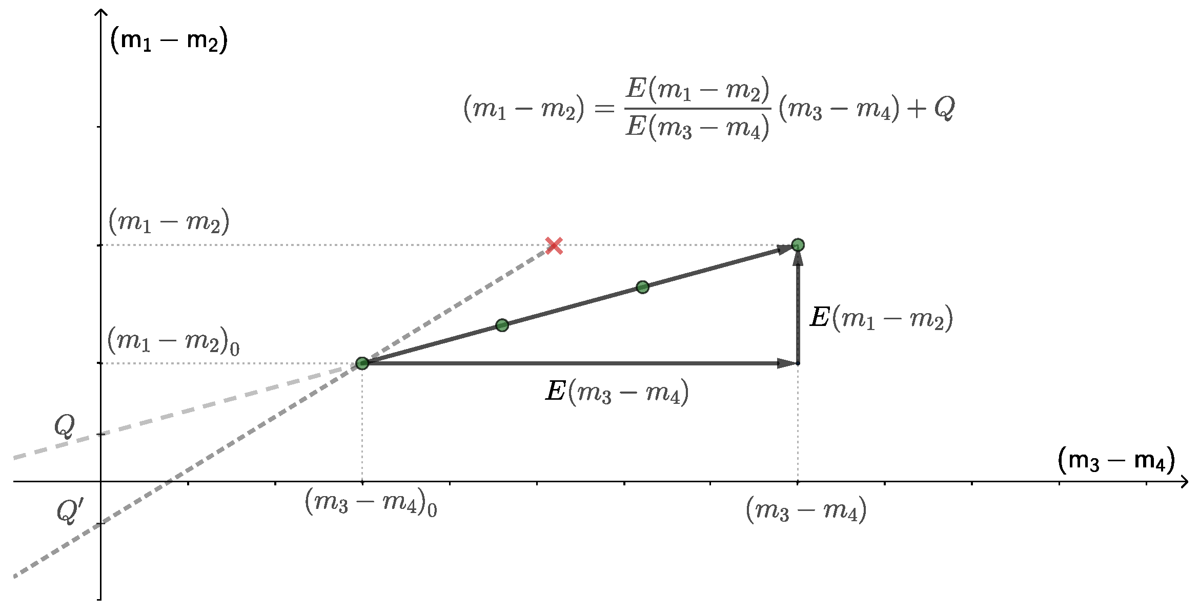
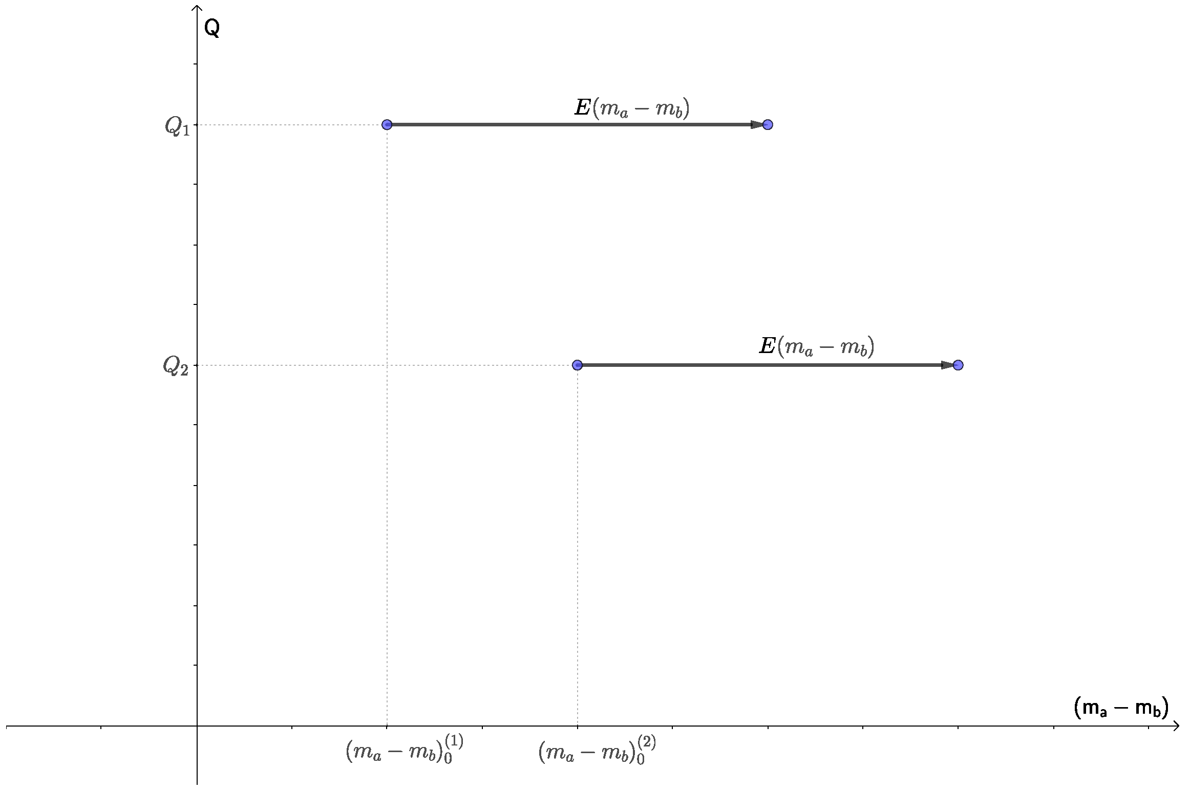
2. Reddening-Free Q Parameter

In the ( U B ) vs. ( B V ) color–color diagram, Johnson and Morgan [25] noted that the lines connecting reddened and unreddened stars of the same spectral type had very nearly the same slope. Thus, they defined the quantity:
Q U B V = ( U B ) E ( U B ) E ( B V ) ( B V )
that turned out to be an interstellar reddening-free parameter and could be used to determine the spectral types and reddening of stars between B1 and B9, inclusive (as explained by Johnson and Morgan [25]).
The definition of the reddening-free Q parameter can be extended to any other photometric system:
Q m 1 m 2 m 3 m 4 = ( m 1 m 2 ) E ( m 1 m 2 ) E ( m 3 m 4 ) ( m 3 m 4 )
considering either four different magnitudes ( m 1 , m 2 , m 3 , and m 4 ) corresponding to different photometric filters or three different magnitudes (adopting m 2 = m 3 ).
The knowledge of the slope, E ( m 1 m 2 ) / E ( m 3 m 4 ) , in the ( m 1 m 2 ) vs. ( m 3 m 4 ) CCD enables elimination of the effect of interstellar reddening and derives the intrinsic color indices of stars. Thus, Q represents the ordinate to the origin of the line connecting the reddened and unreddened positions of each star; see green circles in Figure 1.
On the other hand, the interstellar absorption at a given magnitude, i.e., A m 2 for the m 2 magnitude, as well as the ratio E ( m 1 m 2 ) / E ( m 3 m 4 ) , both depend on the interstellar extinction law1. However, dust extinction has different properties in different regions of the sky, on both small and large scales. Therefore, variations in the interstellar medium (ISM) law would affect not only the color-excess ratios but also the Q parameters [36,37]. This change is represented by:
Δ Q = Q Q = E ( m 1 m 2 ) E ( m 3 m 4 ) anomalous E ( m 1 m 2 ) E ( m 3 m 4 ) normal ( m 3 m 4 )
as shown in Figure 1. Thus, the changes of Q due to different E ( m 1 m 2 ) / E ( m 3 m 4 ) ratios may help to detect the peculiarity of the extinction law towards particular sky regions.
It is interesting to note that in a QCD, stars with the same spectral type, but different “normal” reddening, lie on a straight line parallel to the x-axis, as shown in Figure 2. By using an appropriate set of photometric filters, e.g., the automated two-dimensional classification from multicolor photometry in the Vilnius system [38,39,40,41,42], it would be possible to make a stellar classification with a set of reddening-free Q parameters.
To calculate the standard error ( σ Q ), we should consider that the Q parameter depends on the accuracy of the magnitudes and the color-excess ratio. Thus,
σ Q 2 = σ m 1 2 + σ m 2 2 + E ( m 1 m 2 ) E ( m 3 m 4 ) 2 σ m 3 2 + σ m 4 2 + ( m 3 m 4 ) 2 σ E 2
where E = E ( m 1 m 2 ) / E ( m 3 m 4 ) . Then, considering that the accuracy of all magnitudes is the same, σ m , and σ E = 0 , it results in:
σ Q 2 = 2 σ m 2 1 + E ( m 1 m 2 ) E ( m 3 m 4 ) 2 .

3. Study of Gaia and 2MASS Reddening-Free Q Parameters

We chose to work with Gaia EDR3 [35] and 2MASS [32,33] catalogs because the corresponding missions surveyed the entire sky. Furthermore, B-type stars and nearby stars have unsaturated magnitudes. In this way, we had, in the visual and NIR regions, respectively, the G B p (blue) and G R p (red) passbands of the Gaia system and the 2MASS J, H, and K s photometric bands. We denote, for simplicity, the Gaia B p and R p bands. We did not use the Gaia G-band because, in such a high bandwidth, the extinction coefficient varies strongly with temperature and the extinction itself but less with surface gravity and metallicity [43,44].

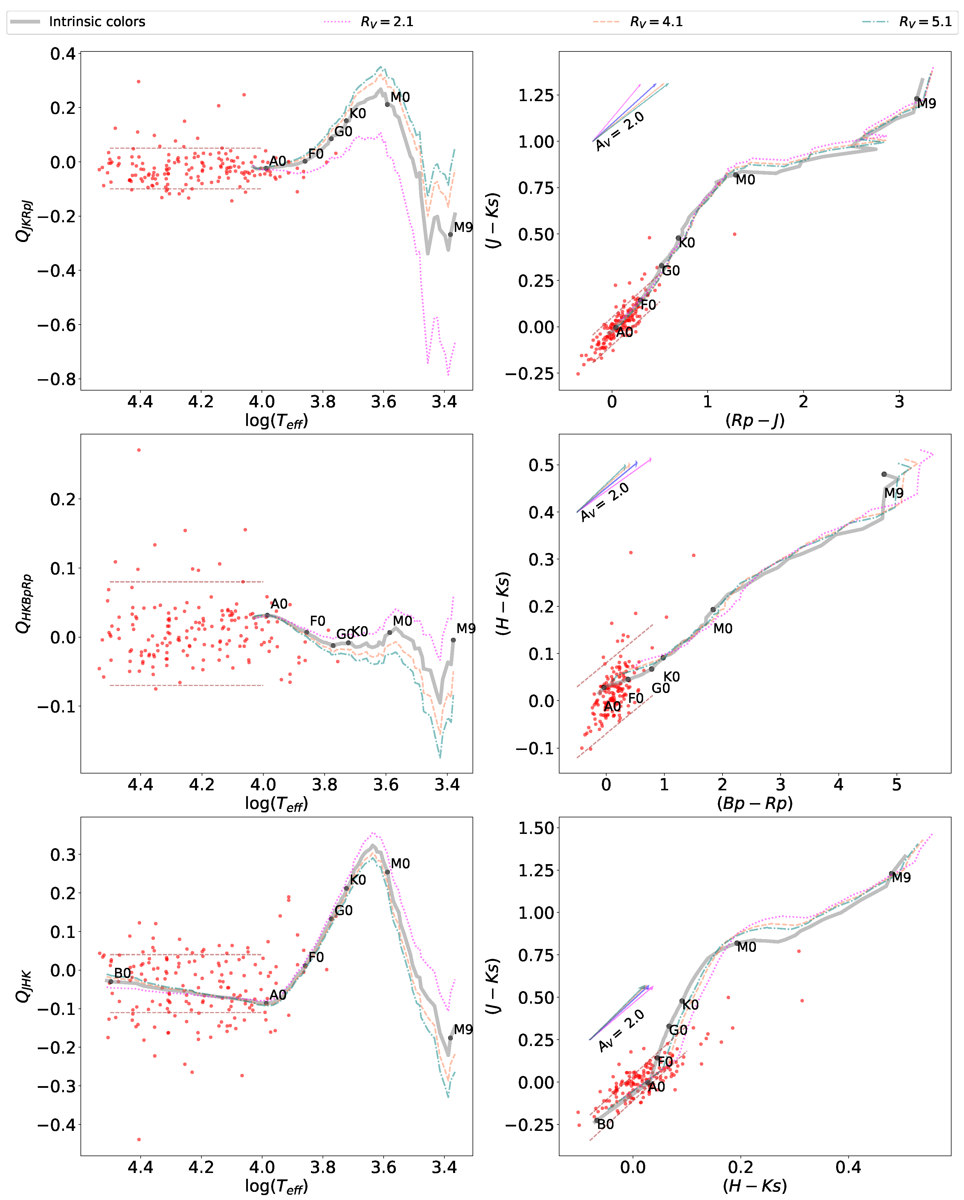
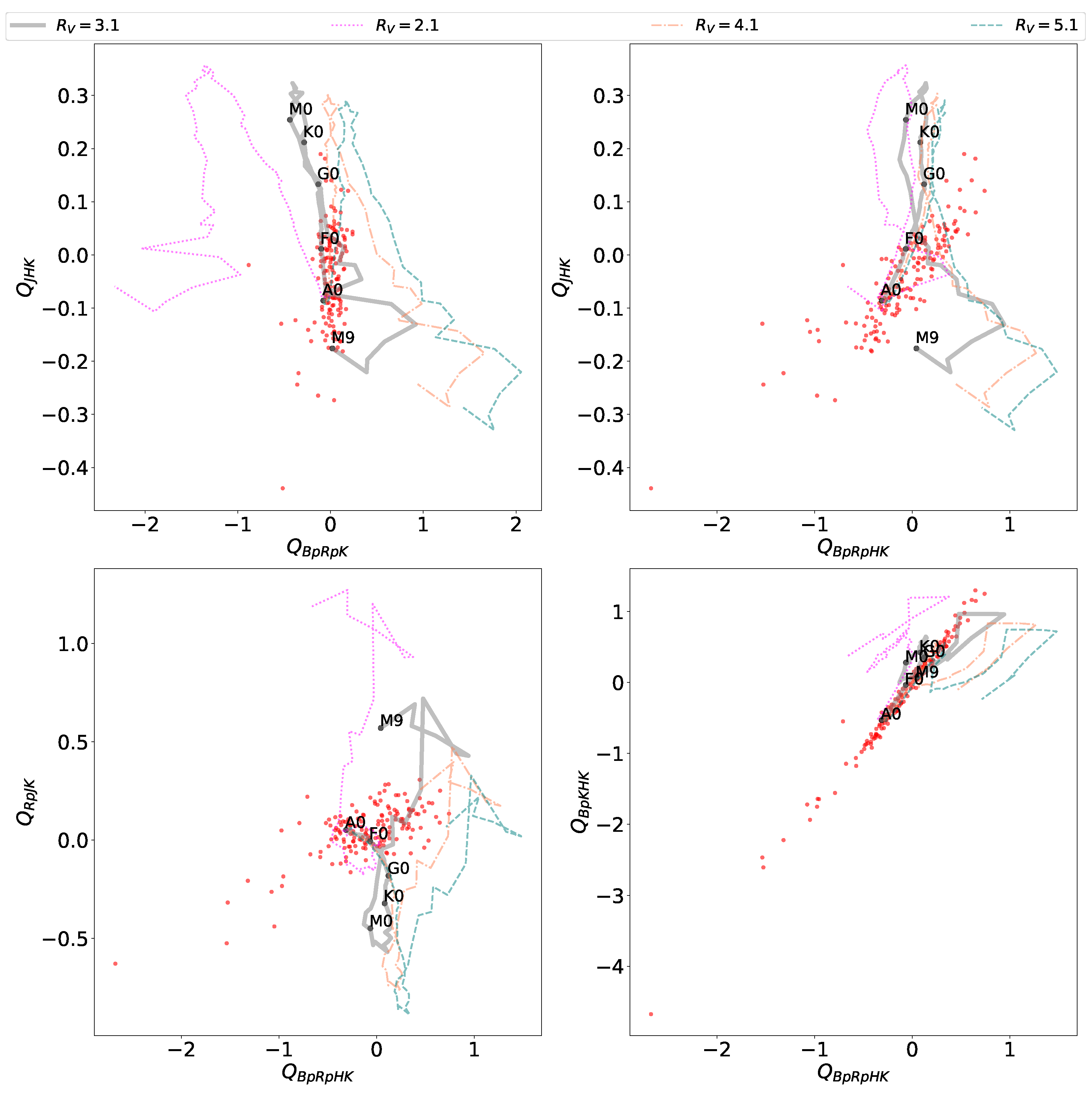
3.1. The Q Parameters and Color-Color Diagrams for Normal B-Type Stars

Since there is no previous study of Q parameters that combine the Gaia and 2MASS photometry, we needed, first, to analyze the position of the B-type stars without emission lines (from now on normal B-type stars) in the different diagrams, Q vs. effective temperature ( T eff ), and their corresponding color–color relations.
The sample of “normal” B-type stars was selected from Zorec et al. [45], Zorec et al. [46], Aidelman et al. [47], Aidelman et al. [48], Aidelman et al. [49] and Cochetti et al. [50]. Our sample did not consider stars classified as Be (that at least once presented the H α line in emission) or Bn (with hydrogen lines deformed by high rotation). This was a homogeneous sample with confident stellar parameters obtained with the spectrophotometric BCD classification system [46,51,52]. The BCD system has a relevant advantage; the photospheric Balmer discontinuity, D , is not affected by interstellar extinction or circumstellar effects (extinction or emission). The reason for this is that the D value is a linear combination of the Q U B V parameter [53].
The cross-matches between the B-type star sample and the Gaia EDR3 and 2MASS catalogs were done using topcat2 (Tool for OPerations on Catalogs And Tables [54,55]). The search radius was set at 0.2 arcsec to avoid duplicated sources. We also selected stars with accurate photometry. This meant they satisfied the following criteria: (a) the magnitude G < 16 mag, (b) mean errors in B p and R p little than 0.01 mag for the Gaia EDR3, and (c) J H K s photometry with quality flags (“Qfl” or “ph_qual”) equal “AAA” for the 2MASS. In this way, we guaranteed that the σ m i contributions at σ Q (in Equation (4)) were as small as possible.
To calculate the reddening-free Q values (Equation (2)) we used the combination of all color indices: ( B p R p ) , ( B p J ) , ( B p H ) , ( B p K s ) , ( R p J ) , ( R p H ) , ( R p K s ) , ( J H ) , ( J K s ) , and ( H K s ) , which led to a total of C ( 10 , 2 ) = 10 ! 2 ! ( 10 2 ) ! = 45 Q parameters. The color-excess ratios were obtained from the relative absorption coefficients, r m a = A m a / A V , for each of the selected five bands, which were estimated using the “extinction” code Fast Interstellar Dust Extinction Laws in Python3 [56]. With this tool, we estimated the r m a values for different wavelengths and different extinction laws for each of the three available models [57,58,59], which also permitted the use of different values for R V . These values are given in Table 2. This code also calculated the extinction for Fitzpatrick and Massa [60]’s model but only for R V = 3.1 . Therefore, this last model was not adopted in this work. It is important to stress that the dependence of B p and R p relative absorption coefficients with the T eff are still unknown. However, as the filters were narrower than the one of the G band, we would expect a lower effect.
In order to estimate typical Q errors for normal B-type stars, we calculated Δ Q and σ Q (Equations (3) and (4), respectively). On the one hand, we estimated | Δ Q | where the Q values were calculated using Fitzpatrick’s model for R V = 2.1 , 4.1 , and 5.1 while the Q values corresponded to R V = 3.1 . On the other hand, we calculated σ Q for each reddening law (see Table 2) using R V = 3.1 and σ E = 0 . Both | Δ Q | and σ Q values were calculated for the 45 combinations of color-excess ratios corresponding to our entire sample of normal B-type stars. These values are shown in Figure 3. The results showed that the mean values were: | Δ Q | 0.05 and σ Q 0.15 . Therefore, any star would show anomalous reddening if its | Q | value was larger than 3 | Δ Q | 0.15 of the expected one for its spectral type. By analogy, we could define a Q range of 3 σ Q 0.45 that would contain all the normal B-type stars. This criterion could be used to identify peculiar stars since they would be located outside the defined Q range.
Figure 4 shows some examples of the behavior of the parameter Q with T eff and their respective color–color indices. These diagrams were selected considering the color indices frequently used in the literature. To study this behavior, we plotted our B-type star sample, together with the main sequence (MS) taken from the Modern Mean Dwarf Stellar Color and Effective Temperature Sequence4 (much of the content of this table, but not all, was incorporated into the Table 5 of [61]). The Q values for both the B star sample (red points) and the MS (solid gray line) were calculated using the model created by Fitzpatrick [59] with R V = 3.1 . To show the effect of anomalous and normal reddening on color–color diagrams, the MS was reddened considering A V = 1 mag, adopting the model done by Fitzpatrick [59] for the different R V coefficients listed in Table 2, while in the Q- T eff diagrams the Q values for MS were calculated also using the Fitzpatrick’s model with R V = 2.1 , 4.1 , and 5.1 (solid and dashed lines, see the caption to Figure 4). Then, considering that σ Q = 0.15 (as set out above), we could define the following limits in the Q- T eff diagrams and CCDs (shown in brown dashed lines):
0.10 Q J K R p J 0.05
0.07 Q H K B p R p 0.08
0.11 Q J H K 0.04
that encloses almost all the B-type stars of the sample (around 86 % , 93 % , and 64 % of a total of 163 stars for each of the limits defined above).

3.2. The Q–Color and QQ Diagrams for Normal B-Type Stars

Generally, the effective temperature of the B-type stars is a priori an unknown quantity and is often derived from spectroscopic data. Therefore, an alternative way to describe the behavior of the Q parameters with T eff , or the spectral types, is to use the color indices. Thus, the ( B p R p ) color index is useful, for example, to classify stars according to their T eff . Jordi et al. [43] remarked that ( B p R p ) plays the same role as ( V I C ) , thus the relationship between ( B p R p ) and T eff could be almost equivalent to the well-known relation of T eff = f ( V I C ) . On the other hand, Mucciarelli et al. [62] also found that ( B p K s ) 0 and ( G K s ) 0 were the best choice to derive precise and accurate T eff values among late-type stars.
Then, to explore the behavior of Q parameters with the color indices, we present some QCD in Figure 5. The Q parameters for the sample of B-type stars and the MS were constructed as explained in Section 3.1. In these plots, the MS was also reddened. These diagrams allowed early-type stars (red cloud of points) to be separated from late types on the MS. In particular, in the Q B p J R p K vs. ( J K s ) and Q B p R p H K vs. ( B p R p ) diagrams (left panels), the B-type stars were located in a well-delimited region. This group was located at
0.11 < Q B p J R p K < 0.20 and 0.20 < ( J K s ) < 0.14
0.60 < Q B p R p H K < 0.50 and 0.30 < ( B p R p ) < 0.40
where the upper limits for the color indices correspond to an F0 V star. Another relevant characteristic of the diagrams of Figure 4 and Figure 5 is that the differences between the MS and anomalous reddening ones seemed to be very small, at least for the selected B-type star group.
Our sample of B-type stars in the Q B p K J H vs. ( B p K s ) diagram (top-right panel of Figure 5) was located in the range 0.17 < Q B p K J H < 1.0 , where the lower limit corresponded to the position of an F0 V-type star. This region could be compared with that defined by Poggio et al. [63] in the ( J H ) vs. ( G DR 2 K s ) . These authors made a preliminary selection of OB candidates that satisfied both ( J H ) < 0.14 ( G DR 2 K s ) + 0.02 and ( J K s ) < 0.23 ( G DR 2 K s ) . The first condition could be expressed in terms of Q as Q J H G DR 2 K = ( J H ) 0.14 ( G DR 2 K s ) < 0.02 . Then, by multiplying both sides by ( 0.14 ) 1 , we obtained Q G DR 2 K J H = ( G DR 2 K s ) 0.07 ( J H ) > 0.14 which was similar to the region defined for Q B p K J H .
As was already mentioned in Section 2, the reddening vector in the QCD has a horizontal direction (Figure 2), for this reason, the reddened B-type stars were overplotted to A and F-type MS stars. This effect was more evident in the Q J H K vs. ( H K s ) diagram (bottom-right panel of Figure 5).
Finally, Figure 6 shows other examples of QQDs. Here, we find that in the Q J H K vs. Q B p R p K (top-left panel) and Q R p J K vs. Q B p R p H K (bottom-left panel) diagrams, the loci of the B-type stars were restricted to a small region around the coordinate point ( 0 , 0 ) :
0.18 < Q J H K < 0.01 and 0.12 < Q B p R p K < 0.18
0.05 < Q R p J K < 0.24 and 0.6 < Q B p R p H K < 0.7
These relations could be used as possible criteria for selecting B-type stars. In particular, the first diagram is very sensitive to the ISM reddening law, and it could also be helpful for detecting stars with anomalous reddening.
On the other hand, the combination of parameters Q J H K vs. Q B p R p H K and Q B p K H K vs. Q B p R p H K (right panels) were not convenient at all, since they mixed late- and early-type stars. Notwithstanding, it drew attention to the fact that the B-type stars were located in a very narrow line that was almost perpendicular to the reddening direction.

4. B-Type Stars with Emission Lines

In the previous section, using several Gaia and 2MASS color–color, Q–color, and QQ diagrams, we delimited regions where normal B-type stars locate. In this section, we analyzed the location in the color–color, Q–color, and QQ diagrams of different kinds of emission-line B-type stars with respect to the normal ones. Our goal was to be able to find criteria that would allow us to separate among the diverse groups of stars with emission lines.
To analyze the position of the emission-line B-type stars in the different diagrams, we constructed our sample using stars classified by Lamers et al. [7], Kraus [12], Miroshnichenko [14], Cidale et al. [20], Oksala et al. [22], Zorec et al. [45], Zorec et al. [46], Aidelman et al. [47], Aidelman et al. [48], Aidelman et al. [49], Cochetti et al. [50], Clark et al. [64] and Guzmán-Díaz et al. [65]. In this way, in addition to the 163 normal B-type stars already studied, our sample was composed of 84 classical Be stars (CBe), 204 HAeBe and HAeB[e] stars, 33 LBVs, and 23 B[e]SGs. We searched for Gaia and 2MASS photometric data, and, finally, we obtained a sample of 156 emission-line B-type stars. It was striking that only 34 HAeBe stars, among the 204 selected stars, had photometric data in the Gaia EDR3 and 2MASS catalogs.

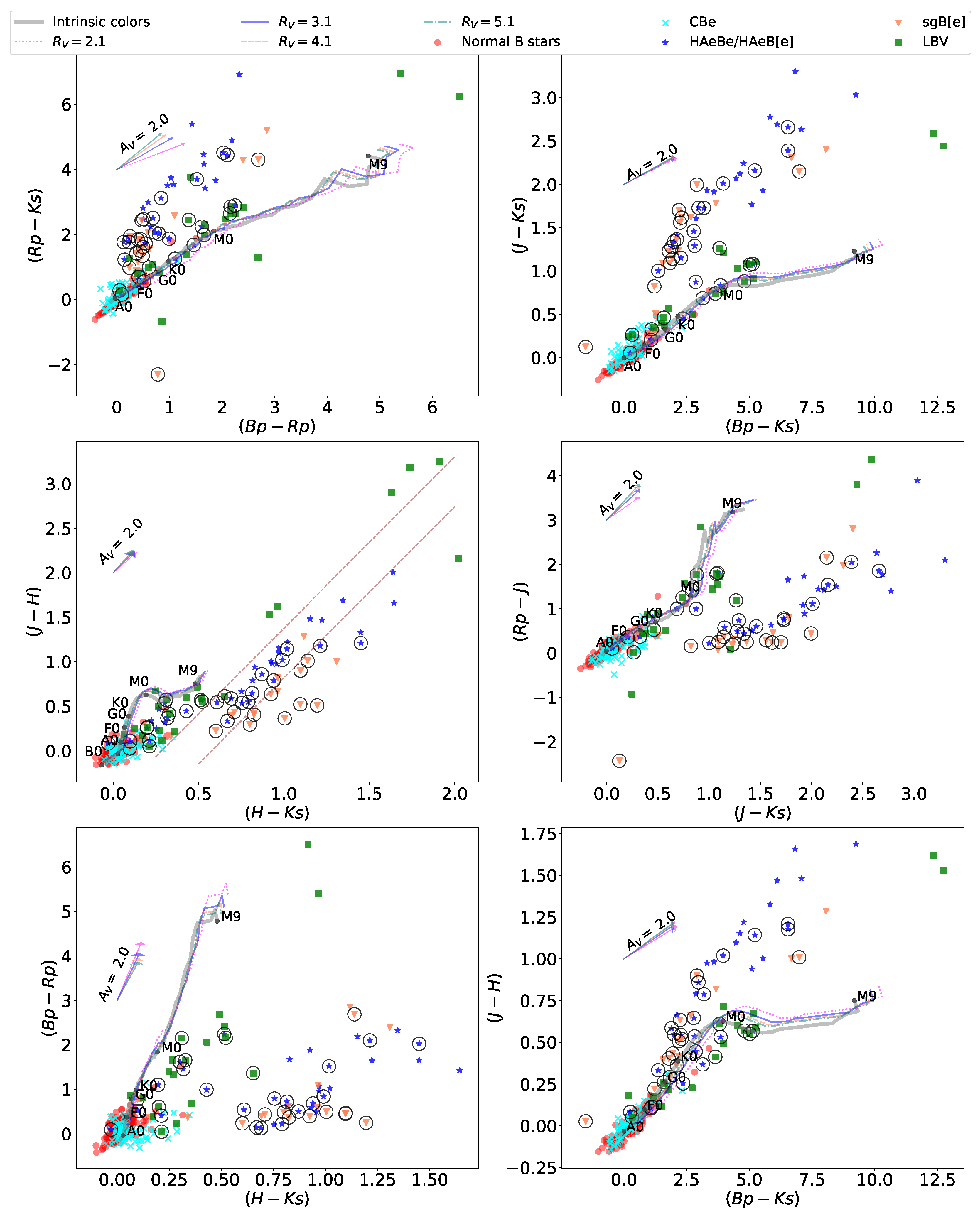
4.1. Color–Color Diagrams for Emission-Line B-Type Stars
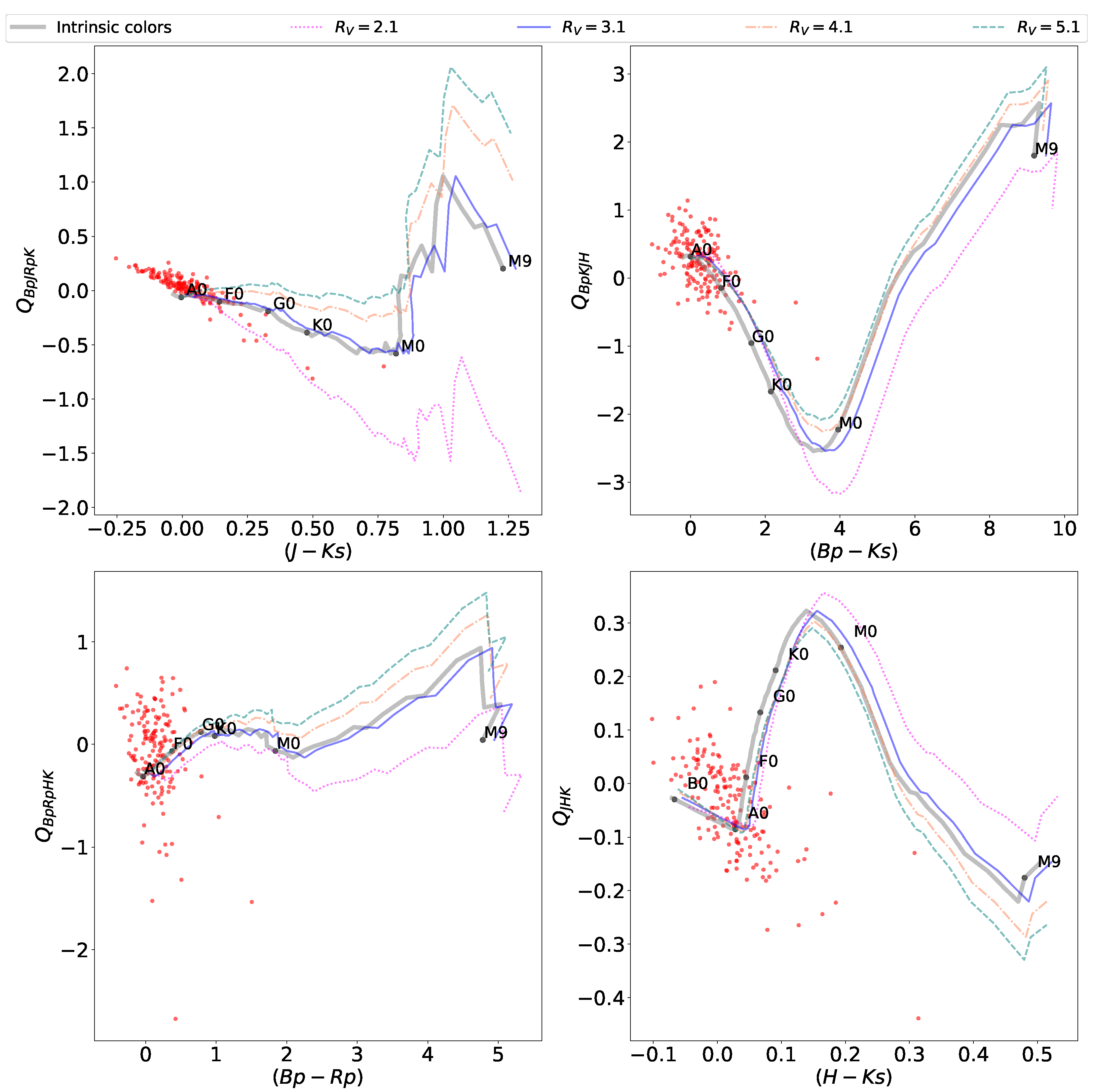
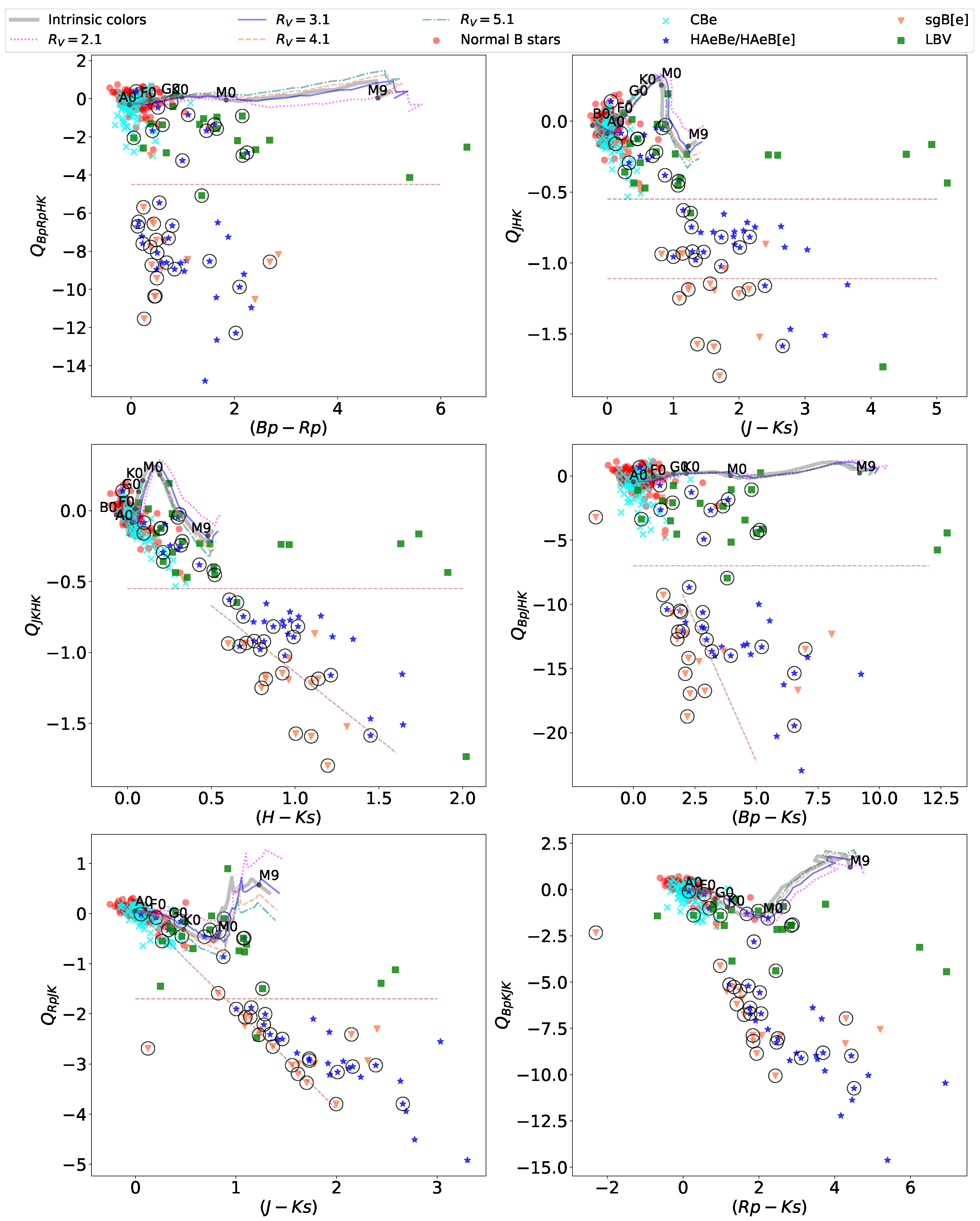
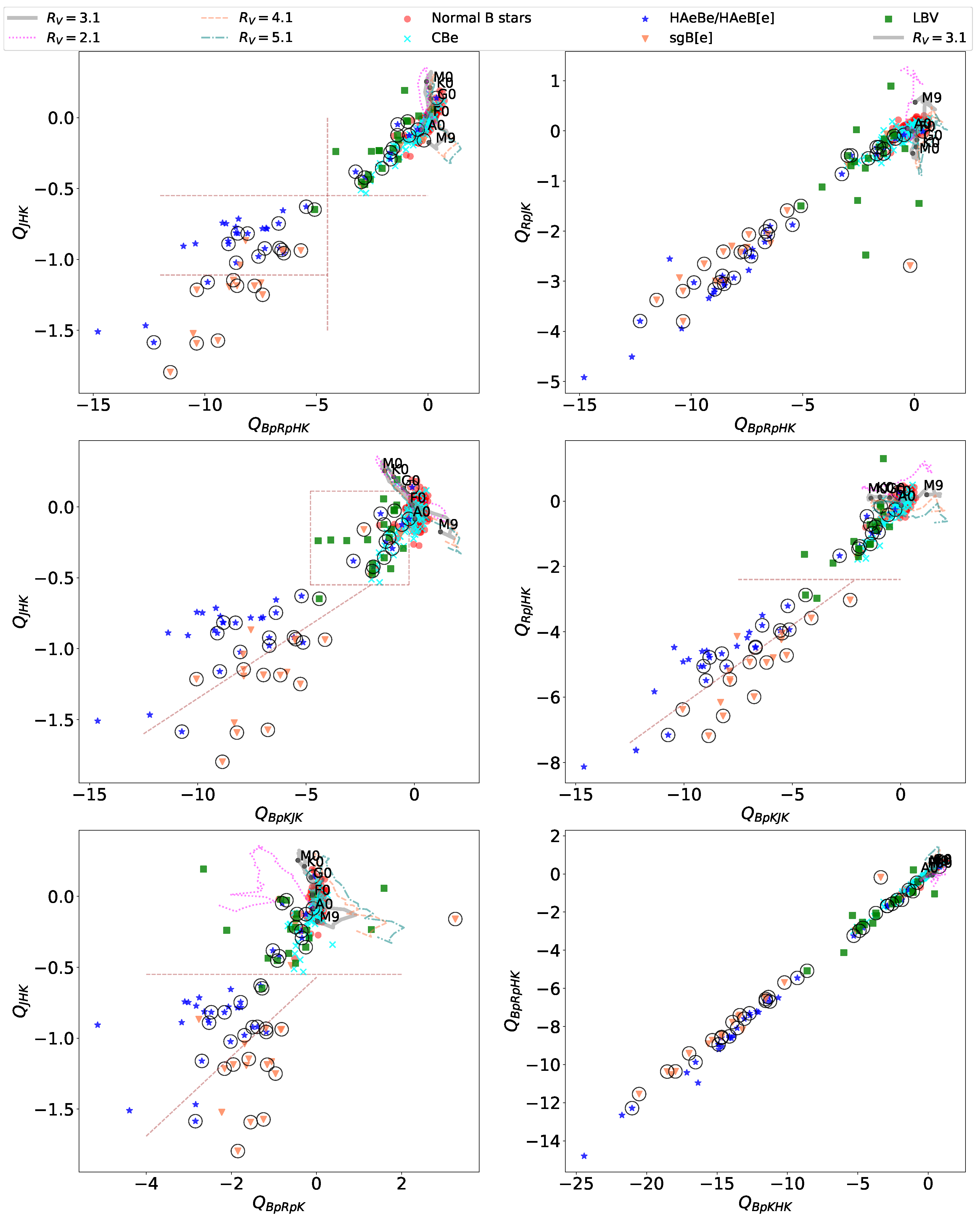
The Gaia and 2MASS color–color diagrams are shown in Figure 7. Again, the solid gray line is the main sequence. The reddening vector ( A v = 2 mag) is indicated in the upper left. The cloud of red and cyan points are, respectively, the normal B and CBe stars. Blue symbols are for HAeBes (and a few HAeB[e]s), orange triangles for B[e]SGs, and green squares for LBVs. Symbols surrounded by black open circles correspond to stars with accurate photometry. These stars satisfied the stated criteria (a), (b), and (c) in Section 3.1. We distinguished two groups of CBe stars in all the plots. The first group behaved as normal B-type stars do. These stars seemed to have small or no infrared excess. The second group encompassed stars with a large color excess, sharing similar photometric characteristics to some LBV stars. These CBe stars presented interstellar reddening and intrinsic color excesses (because the reddening vector points toward a slightly different direction). The large color excess observed in the last group of stars is discussed in Section 5. Particularly interesting are the ( R p K s ) vs. ( B p R p ) and ( J K s ) vs. ( B p K s ) diagrams (top-left and top-right panels in Figure 7, respectively). These are very useful for searching for CBe stars with large infrared excesses because the normal B stars distribute along a narrow and well-defined band.
The best studied NIR color–color diagram in the literature is the ( J H ) vs. ( H K s ) (see Figure 7, middle-left panel). Even when the stars are affected by reddening, this NIR two-color diagram permits separate LBVs from B[e]SG stars [22,23]. However, there is still significant contamination between LBVs and HAeBe stars. This diagram also allows distinguishing, although some mix is observed; the HAeBe stars from both the CBe stars [66] and the B[e]SGs [23]. For illustrative purposes, two straight brown dashed lines ( ( J H ) = 1.93 ( H K s ) 1.11 and ( J H ) = 1.93 ( H K s ) 0.55 ) were plotted to indicate the regions mostly occupied by each group of stars: LBVs, HAeBes and B[e]SGs. Similarly, a ( J H ) vs. ( B p K s ) diagram (Figure 7, bottom-right panel) shows some mixture between young and evolved emission-line stars.
A relevant result was the behavior of the two-color diagram ( B p R p ) vs. ( H K s ) (Figure 7, bottom-left panel), which separated groups of stars (but without recognizing their evolutionary stages) in regions or bands of different color excesses. This behavior was not caused by the reddening vector, which pointed almost perpendicularly to the horizontal shift shown for the different groups of stars. Moreover, this color–color diagram also separated the LBVs from the MS late-type stars. Similarly, the ( R p J ) vs. ( J K s ) diagram discriminated, but to lesser degree, LBVs from the other groups. Although, it seemed to gather groups of stars with different circumstellar reddening (Figure 7, middle-right panel).

4.2. Q–Color and QQ Diagrams for Emission-Line B-Type Stars

As shown in Section 4.1, it was very difficult to delimit regions for HAeBe and B[e]SG stars using two-color diagrams. Particularly, in all these diagrams, these two types of stars were, to more or less degree, mixed. The same happened with the population of HAeBe and LBV stars. Part of this degeneracy could be solved using the Q-color and Q-Q diagrams.
Figure 8 presents several examples of QCD. The top-left panel, Q B p R p H K vs. ( B p R p ) located the LBVs over the line cut Q B p R p H K = 4.5 (brown dashed line). Particularly, the Q J H K vs. ( J K s ) diagram (top-right panel) separated the different groups according to the amount of IR emission. The greater the amount of hot dust, the higher the ( H K s ) color index, which implied a more negative value for Q J H K s = ( J H ) E ( J H ) E ( H K s ) ( H K s ) . In addition, the dashed brown lines at Q J H K = 1.11 and Q J H K = 0.55 represent, respectively, the straight lines plotted on the ( J H ) vs. ( H K s ) diagram. According to this, there were three groups of HAeBe stars, one of them located between the main sequence and the line cut Q J H K = 0.55 . It shared its properties with the LBV group of stars. A second group was located within a region with 1.11 < Q J H K < 0.55 , while the last group had properties similar to the B[e]SGs.
The middle-left panel, Q J K H K vs. ( H K s ) , better separated HAeBes from B[e]SGs. There, the HAeBe stars were more reddened than the B[e]SGs. It is also interesting to note that in both Q J H K vs. ( J K s ) and Q J K H K vs. ( H K s ) diagrams, it was possible to distinguish a group of five strongly reddened LBV stars as they were shifted horizontally to the right.
The most interesting diagram was Q B p J H K vs. ( B p K s ) (middle-right panel), which enabled identification of LBV, B[e]SG, and HAeBe stars from each other. Almost all LBVs had Q B p J H K > 7 . The B[e]SG stars were also well-separated from HAeBe by the straight brown dashed line ( Q B p J H K = 4.33 ( B p K s ) 0.57 ) drawn in the figure. However, in a Q R p J K vs. ( J K s ) diagram (bottom-left panel), both CBe and B[e]SG stars seemed to lie on the same straight line ( Q R p J K = 1.99 ( J K s ) + 0.08 ). Instead, the LBVs had values of Q R p J K > 1.7 . The Q B p K J K vs. ( R p K s ) diagram showed similar behavior.
Figure 9 illustrates several examples of QQD. LBVs and B[e]SGs which are clearly apart from each other. In most of these diagrams, the HAeBe stars are also separate from the B[e]SGs. For instance, on a Q J H K vs. Q B p R p H K diagram (top-left panel), most of the LBVs lie on the right of the vertical line at Q B p R p H K = 4.5 and above the horizontal at Q J H K = 0.55 , thereby complementing information given in Figure 8 (top panels). In a diagram Q J H K vs. Q B p K J K (middle-left panel), the LBVs are inside a box delimited by 4.8 < Q B p K J K < 0.25 , and 0.55 < Q J H K < 0.11 . In addition, it is also possible to separate HAeBes from B[e]SGs through the line Q J H K = 0.1 Q B p K J K 0.35 . Finally, the Q J H K vs. Q B p R p K diagram (bottom-left panel) shows similar behavior.
Concerning the panels on the right side, they show a greater mix between the group of stars than the ones on the left side, e.g., in the Q R p J H K vs. Q B p K J K diagram (middle-right panel), the LBVs have values of Q R p J H K > 2.4 , and the HAeBes and B[e]SGs can be separated with the line Q R p J H K = 0.48 Q B p K J K 1.4 .

5. Discussion

Traditionally, the positions of the stars in different photometric diagrams, or even in the HR diagram, have been adopted as selection criteria to classify stars according to their intrinsic properties, memberships in clusters or associations, variability types, etc. In this work, we focused on studying various color–color diagrams, taking advantage of the Gaia and 2MASS photometric surveys as powerful analysis tools to select and classify B-type stars with and without emission lines. Notably, one would expect that the NIR radiation excess emitted from gaseous and dust CEs of early-type stars would show different properties according to their chemical composition (gas-to-dust ratio), the absorption and heating mechanisms of particles, dust temperature, and the size of dust grains. As each diagram has its own limitations, mainly because the colors are affected by ISM, it was important to adopt multiple criteria. For this purpose, we also analyzed different reddening-free Q parameters, since the method presents high confidence. For instance, Mohr-Smith et al. [67] found that the extension of the Q method to the Sloan filter system had a confidence of 97 % . The study was based on follow-up spectroscopy of a sample of OB stars selected in a previous study using the Q method [68].
In general, from the two-color diagrams of Figure 7, the HAeBe stars were very difficult to separate from B[e]SGs or LBVs. The best option was the ( J H ) vs. ( H K s ) diagram that enabled distinguishing HAeBe from B[e]SGs [23], and LVBs from B[e]SGs [22], delimiting particular regions through straight lines (middle-left panel). However, there was still a substantial mixture between the HAeBe stars and the LBVs group (according to [23]). This preliminary classification could be complemented by the information derived from a ( B p R p ) vs. ( H K s ) diagram that permitted, in addition, the identification of hot-HAeBe and B[e]SG stars with strong intrinsic IR emissions and no reddening interstellar excess. These stars were located within a region defined by 0 ( B p R p ) 1 and 0.5 ( H K s ) 1.25 . All this information could also be retrieved in the Q J H K vs. Q B p R p H K diagram, where the straight lines, plotted on the J H K s two-color diagram, were transformed into horizontal lines at Q J H K = 0.55 and Q J H K = 1.11 . The box in the ( B p R p ) vs. ( H K s ) two-color diagram resulted in the range 12.4 Q B p R p H K 3.96 . Furthermore, in this QQD the three groups of stars, that is the HAeBes, LBVs, and B[e]SGs, were well separated from each other. According to Oksala et al. [22], the B[e]SGs were surrounded by larger amounts of hot dust than the LBVs, whereas the LBVs hosted huge amounts of cool dust at far distances.
We also recognized three kinds of HAeBe stars that presented different amounts of NIR radiation excess. In all CCDs, QCDs, and QQDs, we observed a group of HAeBes located in the same region as LBVs and some CBe stars. Figure 9 (top-left panel) shows that this group of stars had Q J H K > 0.55 . The other two groups had 1.11 < Q J H K < 0.55 , and Q J H K < 1.11 , respectively. The latter corresponded to HAeBe stars with significant IR excess. Our result agreed with that found by Chen et al. [19] in a ( J H ) vs. ( H K s ) diagram. These authors noted that the majority of HAeBe stars were located in the region of 0 < ( H K s ) < 2 and 0.2 < ( J H ) < 2.0 , which means 4.08 < Q J H K < 2 . Only a small group of sources presented less or no infrared excess showing a similar distribution as the majority of the CBe stars ( 0.2 < ( H K s ) < 0.2 and 0.2 < ( J H ) < 0.2 ), which implied that 0.59 < Q J H K < 0.59 . Finally, they found sources that had very large infrared excesses with ( H K ) > 1.5 . Sources with less excess IR radiation probably originated from free ionized gas emissions. Instead, those sources with large excesses of IR radiation were likely indicative of the influence of a bright nebulosity related to low temperatures or mainly thermal emissions from the surrounding dust [4].
A somewhat similar result was achieved for the CBe stars. Our sample of CBe stars encompassed bright Be field stars and Galactic cluster members. Among them, we recognized two types of CBe stars. One group, with small near-IR excess, resembled the normal B-type stars. The second group consisted of a few CBe stars (and a small group of stars classified as normal B-type stars) with a moderate IR excess, sharing properties with the LBVs. The latter could be better identified in the QCDs of Figure 8, particularly, in the Q B p R p H K vs. ( B p R p ) (top-left panel) and Q B p J H K vs. ( B p K s ) (middle-right panel) diagrams. Zhang et al. [66] explained that a small radiation excess could be accounted for by hot circumstellar plasma, but a larger IR excess would require thermal emission from circumstellar dust. Lee and Chen [69] proposed that the dust grains were produced by condensation in the expanding stellar atmosphere, and, therefore, the dust particles should be very small in size to reprocess starlight efficiently. In contrast, the HAeBe stars showed a very large infrared excess which arose from relatively large grains as part of surplus star-forming materials. However, Rivinius et al. [5] asserted that dust had never been found in the envelopes of Be stars and that it was precisely the presence of dust that made it possible to distinguish a CBe from a HAeBe. As a consequence, stars with large color excesses are likely misclassified and would not be CBe.

6. Conclusions

This work discussed the properties of different color–color diagrams and equivalent Johnson’s reddening-free Q parameters built using a combination of the Gaia and 2MASS photometry. Although the Q values were free from the ISM reddening effect, they still showed a dependence on the reddening law in the sky region. Nevertheless, using appropriate combinations of color indices, it was possible to minimize this effect among the O, B, and A stars. Furthermore, by analyzing the different diagrams, we were able to establish criteria to identify stars of spectral type B (Equations (6), (9) and (11)), as well as to identify early-type stars with emission lines of different nature. Main selection criteria are summarize in Table 3.
In addition to the well-known ( J H ) vs. ( H K s ) color–color diagram, which is an excellent dust tracer of circumstellar envelopes, we also found that the ( B p R p ) vs. ( H K s ) diagram could be used to identify emission-line B-type stars corrected by interstellar reddening, but with strong intrinsic IR emission. Particularly interesting were the ( R p K s ) vs. ( B p R p ) and ( J K s ) vs. ( B p K s ) diagrams, as they might be helpful to search for CBe stars with large infrared excesses, because the normal B-type stars distribute along a narrow and well-defined band.
The main advantage of the QCDs over the color–color ones was that the B-type stars did not mix with the M-type stars, as shown, particularly in the Q B p R p H K vs. ( B p R p ) , and Q B p J H K vs. ( B p K s ) diagrams. Moreover, early-type stars that have anomalous reddening, due to the presence of circumstellar envelopes, can be easily recognized. This is because the effect of interstellar extinction causes stars of the same spectral types to shift to the right of the diagram. At the same time, the presence of the circumstellar envelope makes the Q value more negative (when using an IR color index). We suggest using different selection criteria, such as those that arise from the Q J K H K vs. ( H K s ) and Q B p J H K vs. ( B p K s ) diagrams, to search for, and classify, B-type stars with emission lines. These diagrams also allow the LBV stars to be well-recognized from HAeBes and B[e]SGs. In addition, the region of the HAeBe stars can be separated from that of the B[e]SG stars by a straight line. However, there was still significant contamination between HAeBes and LBVs, that it would be desirable to get rid of when making source selections.
As was already stressed, QQDs are free from interstellar extinction, although they are sensitive to anomalous reddening. However, the presence of a circumstellar envelope produces a shift of the Q-values in a direction almost perpendicular to the effect of the anomalous reddening. Then, the QQDs are powerful tools to identify stars with intrinsic IR emission.
Using the Q parameters allowed us to recognize two classes of CBe stars. One group resembled the normal B-type stars with small near-IR excess, and the other group had a few objects showing moderate to large IR excess. This second group might show dusty envelopes formed as a result of the evolution and would not be CBe stars. We also detected three kinds of HAeBe stars. The first group had small IR radiation excess. Stars in this group shared properties with CBe stars and LBVs. A second group showed a moderate contribution from dust, and a third group showed a significant IR excess comparable with the properties of B[e]SGs. All these groups need further study to understand their dust grain properties and formation processes.
Thus, based on the location of the stars in different CCDs, QCDs, and QQDs, we were able to state various selection criteria that allowed separating, as much as possible, the diverse groups of B-type stars with a moderate and large IR excess (e.g., CBes, HAeBes, LBVs, and B[e]SGs). Both the diagrams and stated criteria can be very useful tools for automated designs of machine learning and optimal search algorithms.

Author Contributions

Conceptualization, Y.A. and L.S.C.; methodology, Y.A.; formal analysis, Y.A.; investigation, Y.A.; writing—original draft preparation, Y.A. and L.S.C.; writing—review and editing, L.S.C.; visualization, Y.A.; supervision, L.S.C.; funding acquisition, Y.A. and L.S.C. All authors have read and agreed to the published version of the manuscript.

Funding

This research was funded by CONICET (PIP 1337) and the Universidad Nacional de La Plata (Programa de Incentivos 11/G160), Argentina. In addition, this project has received funding from the European Union’s Framework Programme for Research and Innovation Horizon 2020 (2014-2020) under the Marie Skłodowska-Curie Grant Agreement No. 823734.

Data Availability Statement

Not applicable.

Acknowledgments

This publication made use of data products from the Two Micron All Sky Survey, which is a joint project of the University of Massachusetts and the Infrared Processing and Analysis Center/California Institute of Technology, funded by the National Aeronautics and Space Administration and the National Science Foundation. This work presented results from the European Space Agency (ESA) space mission Gaia. Gaia data are being processed by the Gaia Data Processing and Analysis Consortium (DPAC). Funding for the DPAC is provided by national institutions, in particular, the institutions participating in the Gaia MultiLateral Agreement (MLA). The Gaia mission website is https://www.cosmos.esa.int/gaia (the last accessed date was 1 February 2023). The Gaia archive website is https://archives.esac.esa.int/gaia (the last accessed date was 1 February 2023).

Conflicts of Interest

The authors declare no conflict of interest.

Abbreviations

The following abbreviations are used in this manuscript:
CECircumstellar envelope
IRinfrared
HAeBeHerbig Ae/Be star
PMSPre-main sequence star
CBeClassical Be star
BSGB supergiant star
LBVLuminous Blue Variable star
B[e]SGB[e] supergiant star
unclB[e]unclassified B[e] star
NIRnear infrared
CCDColor-color diagram
YSOYoung Stellar Object
GaiaGlobal Astrometric Interferometer for Astrophysics mission
2MASSTwo Micron All Sky Survey
QQDQ-Q diagrams
EDR3Early Data Release 3
QCDQ-color index diagram
ISMInterstellar medium
T eff Effective temperature
TopcatTool for OPerations on Catalogues And Tables
MSMain sequence

Notes

1
The color-excess ratio is E ( m 1 m 2 ) E ( m 3 m 4 ) = A m 1 A m 2 A m 3 A m 4 = R m 1 R m 2 R m 3 R m 4 = r m 1 r m 2 r m 3 r m 4 where R m a and r m a are the relative absorption coefficients referring to the color excess E ( B V ) , R m a = A m a / E ( B V ) , and to the extinction A V , r m a = A m a / A V , respectively.
2
http://www.starlink.ac.uk/topcat/. The last accessed date is 2 January 2023.
3
https://extinction.readthedocs.io/en/latest/. The last accessed date was 2 January 2023.
4
Version 2019.3.22, in http://www.pas.rochester.edu/emamajek/EEM_dwarf_UBVIJHK_colors_Teff.txt. The last accessed date was 2 January 2023.

References

  1. Porter, J.M.; Rivinius, T. Classical Be Stars. Publ. Astron. Soc. Pac. 2003, 115, 1153–1170. [Google Scholar] [CrossRef]
  2. Allen, D.A. Near infra-red magnitudes of 248 early-type emission-line stars and related objects. Mon. Not. R. Astron. Soc. 1973, 161, 145–166. [Google Scholar] [CrossRef] [Green Version]
  3. Herbig, G.H. The Spectra of Be- and Ae-Type Stars Associated with Nebulosity. Astrophys. J. Suppl. Ser. 1960, 4, 337. [Google Scholar] [CrossRef]
  4. Hillenbrand, L.A.; Strom, S.E.; Vrba, F.J.; Keene, J. Herbig Ae/Be Stars: Intermediate-Mass Stars Surrounded by Massive Circumstellar Accretion Disks. Astrophys. J. 1992, 397, 613. [Google Scholar] [CrossRef]
  5. Rivinius, T.; Carciofi, A.C.; Martayan, C. Classical Be stars. Rapidly rotating B stars with viscous Keplerian decretion disks. Astron. Astrophys. Rev. 2013, 21, 69. [Google Scholar] [CrossRef] [Green Version]
  6. Chita, S.M.; Langer, N.; van Marle, A.J.; García-Segura, G.; Heger, A. Multiple ring nebulae around blue supergiants. Astron. Astrophys. 2008, 488, L37–L41. [Google Scholar] [CrossRef] [Green Version]
  7. Lamers, H.J.G.L.M.; Zickgraf, F.J.; de Winter, D.; Houziaux, L.; Zorec, J. An improved classification of B[e]-type stars. Astron. Astrophys. 1998, 340, 117–128. [Google Scholar]
  8. Humphreys, R.M.; Davidson, K. The Luminous Blue Variables: Astrophysical Geysers. Publ. Astron. Soc. Pac. 1994, 106, 1025. [Google Scholar] [CrossRef]
  9. Mehner, A.; Baade, D.; Groh, J.H.; Rivinius, T.; Hambsch, F.J.; Bartlett, E.S.; Asmus, D.; Agliozzo, C.; Szeifert, T.; Stahl, O. Spectroscopic and photometric oscillatory envelope variability during the S Doradus outburst of the luminous blue variable R71. Astron. Astrophys. 2017, 608, A124. [Google Scholar] [CrossRef] [Green Version]
  10. Campagnolo, J.C.N.; Borges Fernandes, M.; Drake, N.A.; Kraus, M.; Guerrero, C.A.; Pereira, C.B. Detection of new eruptions in the Magellanic Clouds luminous blue variables R 40 and R 110. Astron. Astrophys. 2018, 613, A33. [Google Scholar] [CrossRef] [Green Version]
  11. Weis, K.; Bomans, D.J. Luminous Blue Variables. Galaxies 2020, 8, 20. [Google Scholar] [CrossRef]
  12. Kraus, M. A Census of B[e] Supergiants. Galaxies 2019, 7, 83. [Google Scholar] [CrossRef] [Green Version]
  13. Zickgraf, F.J.; Schulte-Ladbeck, R.E. Polarization characteristics of galactic Be stars. Astron. Astrophys. 1989, 214, 274–284. [Google Scholar]
  14. Miroshnichenko, A.S. Toward Understanding the B[e] Phenomenon. I. Definition of the Galactic FS CMa Stars. Astrophys. J. 2007, 667, 497–504. [Google Scholar] [CrossRef] [Green Version]
  15. Kwok, S. Proto-planetary nebulae. Annu. Rev. Astron. Astrophys. 1993, 31, 63–92. [Google Scholar] [CrossRef]
  16. Klement, R.; Carciofi, A.C.; Rivinius, T.; Matthews, L.D.; Vieira, R.G.; Ignace, R.; Bjorkman, J.E.; Mota, B.C.; Faes, D.M.; Bratcher, A.D.; et al. Revealing the structure of the outer disks of Be stars. Astron. Astrophys. 2017, 601, A74. [Google Scholar] [CrossRef] [Green Version]
  17. Oudmaijer, R.D. The B[e] Phenomenon in Pre-Main-Sequence Herbig Ae/Be Stars. In Proceedings of the The B[e] Phenomenon: Forty Years of Studies, Prague, Czech Republic, 27 June–1 July 2016; Miroshnichenko, A., Miroshnichenko, A., Zharikov, S., Korčáková, D., Wolf, M., Eds.; Astronomical Society of the Pacific Conference Series. Astronomical Society of the Pacific: California, CA, USA, 2017; Volume 508, p. 175. [Google Scholar]
  18. Sheikina, T.A.; Miroshnichenko, A.S.; Corporon, P. B-type Emission-line Stars with Warm Circumstellar Dust. In Proceedings of the IAU Colloq. 175: The Be Phenomenon in Early-Type Stars, Alicante, Spain, 28 June–2 July 1999; Smith, M.A., Henrichs, H.F., Fabregat, J., Eds.; Astronomical Society of the Pacific Conference Series. Astronomical Society of the Pacific: California, CA, USA, 2000; Volume 214, p. 494. [Google Scholar]
  19. Chen, P.S.; Shan, H.G.; Zhang, P. A new photometric study of Herbig Ae/Be stars in the infrared. New Astron. 2016, 44, 1–11. [Google Scholar] [CrossRef]
  20. Cidale, L.; Zorec, J.; Tringaniello, L. BCD spectrophotometry of stars with the B[e] phenomenon. I. Fundamental parameters. Astron. Astrophys. 2001, 368, 160–174. [Google Scholar] [CrossRef]
  21. Comerón, F.; Pasquali, A.; Rodighiero, G.; Stanishev, V.; De Filippis, E.; López Martí, B.; Gálvez Ortiz, M.C.; Stankov, A.; Gredel, R. On the massive star contents of Cygnus OB2. Astron. Astrophys. 2002, 389, 874–888. [Google Scholar] [CrossRef] [Green Version]
  22. Oksala, M.E.; Kraus, M.; Cidale, L.S.; Muratore, M.F.; Borges Fernandes, M. Probing the ejecta of evolved massive stars in transition. A VLT/SINFONI K-band survey. Astron. Astrophys. 2013, 558, A17. [Google Scholar] [CrossRef] [Green Version]
  23. Cochetti, Y.R.; Kraus, M.; Arias, M.L.; Cidale, L.S.; Eenmäe, T.; Liimets, T.; Torres, A.F.; Djupvik, A.A. Near-infrared Characterization of Four Massive Stars in Transition Phases. Astron. J. 2020, 160, 166. [Google Scholar] [CrossRef]
  24. Negueruela, I.; Schurch, M.P.E. A search for counterparts to massive X-ray binaries using photometric catalogues. Astron. Astrophys. 2007, 461, 631–639. [Google Scholar] [CrossRef]
  25. Johnson, H.L.; Morgan, W.W. Fundamental stellar photometry for standards of spectral type on the Revised System of the Yerkes Spectral Atlas. Astrophys. J. 1953, 117, 313. [Google Scholar] [CrossRef]
  26. Comerón, F.; Pasquali, A. The ionizing star of the North America and Pelican nebulae. Astron. Astrophys. 2005, 430, 541–548. [Google Scholar] [CrossRef] [Green Version]
  27. Bessell, M.S.; Brett, J.M. JHKLM Photometry: Standard Systems, Passbands, and Intrinsic Colors. Publ. Astron. Soc. Pac. 1988, 100, 1134. [Google Scholar] [CrossRef]
  28. Garcia, M.; Herrero, A.; Castro, N.; Corral, L.; Rosenberg, A. The young stellar population of IC 1613. II. Physical properties of OB associations. Astron. Astrophys. 2010, 523, A23. [Google Scholar] [CrossRef]
  29. Aparicio Villegas, T.; Alfaro, E.J.; Cabrera-Caño, J.; Moles, M.; Benítez, N.; Perea, J.; del Olmo, A.; Fernández-Soto, A.; Cristóbal-Hornillos, D.; Aguerri, J.A.L.; et al. Stellar physics with the ALHAMBRA photometric system. J. Phys. Conf. Ser. 2011, 328, 012004. [Google Scholar] [CrossRef]
  30. Gaia Collaboration; Prusti, T.; de Bruijne, J.H.J.; Brown, A.G.A.; Vallenari, A.; Babusiaux, C.; Bailer-Jones, C.A.L.; Bastian, U.; Biermann, M.; Evans, D.W.; et al. The Gaia mission. Astron. Astrophys. 2016, 595, A1. [Google Scholar] [CrossRef] [Green Version]
  31. Gaia Collaboration; Brown, A.G.A.; Vallenari, A.; Prusti, T.; de Bruijne, J.H.J.; Mignard, F.; Drimmel, R.; Babusiaux, C.; Bailer-Jones, C.A.L.; Bastian, U.; et al. Gaia Data Release 1. Summary of the astrometric, photometric, and survey properties. Astron. Astrophys. 2016, 595, A2. [Google Scholar] [CrossRef] [Green Version]
  32. Cutri, R.M.; Skrutskie, M.F.; van Dyk, S.; Beichman, C.A.; Carpenter, J.M.; Chester, T.; Cambresy, L.; Evans, T.; Fowler, J.; Gizis, J.; et al. 2MASS All Sky Catalog of Point Sources. 2003. Available online: https://vizier.cds.unistra.fr/viz-bin/VizieR?-source=II/246 (accessed on 2 January 2023).
  33. Skrutskie, M.F.; Cutri, R.M.; Stiening, R.; Weinberg, M.D.; Schneider, S.; Carpenter, J.M.; Beichman, C.; Capps, R.; Chester, T.; Elias, J.; et al. The Two Micron All Sky Survey (2MASS). Astron. J. 2006, 131, 1163–1183. [Google Scholar] [CrossRef]
  34. Straizys, V.; Lazauskaite, R.; Liubertas, R.; Azusienis, A. Star Classification Possibilities with Broad-Band Photometric Systems. I. The Sloan System. Balt. Astron. 1998, 7, 605–623. [Google Scholar] [CrossRef]
  35. Gaia Collaboration; Brown, A.G.A.; Vallenari, A.; Prusti, T.; de Bruijne, J.H.J.; Babusiaux, C.; Biermann, M.; Creevey, O.L.; Evans, D.W.; Eyer, L.; et al. Gaia Early Data Release 3. Summary of the contents and survey properties. Astron. Astrophys. 2021, 649, A1. [Google Scholar] [CrossRef]
  36. Johnson, H.L.; Morgan, W.W. Some Evidence for a Regional Variation in the Law of Interstellar Reddening. Astrophys. J. 1955, 122, 142. [Google Scholar] [CrossRef]
  37. Straižys, V. Multicolor Stellar Photometry; Pachart Pub. House: Tucson, AZ, USA, 1992. [Google Scholar]
  38. Bartkevicius, A.; Zdanavicius, K. Calculation of reddening-free parameters Q of the Vilnius photometric system by the iteration method. Vilnius Astron. Obs. Biul. 1975, 41, 30. [Google Scholar]
  39. Pucinskas, A. Photographic photometry of stars in the region of open cluster IC 4996 in the Vilnius photometric system. Vilnius Astron. Obs. Biul. 1982, 59, 3. [Google Scholar]
  40. Jasevicius, V. Photometric quantification of stars in the Vilnius system using the method of independent Q parameters. Vilnius Astron. Obs. Biul. 1986, 74, 40. [Google Scholar]
  41. Smriglio, F.; Boyle, R.P.; Straizys, V.; Janulis, R.; Nandy, K.; MacGillivray, H.T.; McLachlan, A.; Coluzzi, R.; Segato, C. Automated two-dimensional classification from multicolour photometry in the Vilnius system. Astron. Astrophys. 1986, 66, 181–190. [Google Scholar]
  42. Smriglio, F.; Dasgupta, A.K.; Nandy, K.; Boyle, R.P. A comparison of automated spectral classification using Vilnius photometry with MK classification. Astron. Astrophys. 1990, 228, 399–402. [Google Scholar]
  43. Jordi, C.; Gebran, M.; Carrasco, J.M.; de Bruijne, J.; Voss, H.; Fabricius, C.; Knude, J.; Vallenari, A.; Kohley, R.; Mora, A. Gaia broad band photometry. Astron. Astrophys. 2010, 523, A48. [Google Scholar] [CrossRef] [Green Version]
  44. Danielski, C.; Babusiaux, C.; Ruiz-Dern, L.; Sartoretti, P.; Arenou, F. The empirical Gaia G-band extinction coefficient. Astron. Astrophys. 2018, 614, A19. [Google Scholar] [CrossRef] [Green Version]
  45. Zorec, J.; Frémat, Y.; Cidale, L. On the evolutionary status of Be stars. I. Field Be stars near the Sun. Astron. Astrophys. 2005, 441, 235–248. [Google Scholar] [CrossRef] [Green Version]
  46. Zorec, J.; Cidale, L.; Arias, M.L.; Frémat, Y.; Muratore, M.F.; Torres, A.F.; Martayan, C. Fundamental parameters of B supergiants from the BCD system. I. Calibration of the (λ_1, D) parameters into Teff. Astron. Astrophys. 2009, 501, 297–320. [Google Scholar] [CrossRef] [Green Version]
  47. Aidelman, Y.; Cidale, L.S.; Zorec, J.; Arias, M.L. Open clusters. I. Fundamental parameters of B stars in NGC 3766 and NGC 4755. Astron. Astrophys. 2012, 544, A64. [Google Scholar] [CrossRef] [Green Version]
  48. Aidelman, Y.; Cidale, L.S.; Zorec, J.; Panei, J.A., II. Fundamental parameters of B stars in Collinder 223, Hogg 16, NGC 2645, NGC 3114, and NGC 6025. Astron. Astrophys. 2015, 577, A45. [Google Scholar] [CrossRef] [Green Version]
  49. Aidelman, Y.; Cidale, L.S.; Zorec, J.; Panei, J.A. Open clusters. III. Fundamental parameters of B stars in NGC 6087, NGC 6250, NGC 6383, and NGC 6530 B-type stars with circumstellar envelopes. Astron. Astrophys. 2018, 610, A30. [Google Scholar] [CrossRef] [Green Version]
  50. Cochetti, Y.R.; Zorec, J.; Cidale, L.S.; Arias, M.L.; Aidelman, Y.; Torres, A.F.; Frémat, Y.; Granada, A. Be and Bn stars: Balmer discontinuity and stellar-class relationship. Astron. Astrophys. 2020, 634, A18. [Google Scholar] [CrossRef]
  51. Barbier, D.; Chalonge, D. Étude du rayonnement continu de quelques étoiles entre 3 100 et 4 600 Å (4e Partie-discussion générale). Ann. D’Astrophys. 1941, 4, 30. [Google Scholar]
  52. Chalonge, D.; Divan, L. Recherches sur les spectres continus stellaires. V. Etude du spectre continu de 150 etoiles entre 3150 et 4600 A. Ann. D’Astrophys. 1952, 15, 201. [Google Scholar]
  53. Moujtahid, A.; Zorec, J.; Hubert, A.M.; Garcia, A.; Burki, G. Long-term visual spectrophotometric behaviour of Be stars. Astron. Astrophys. 1998, 129, 289–311. [Google Scholar] [CrossRef]
  54. Taylor, M.B. TOPCAT & STIL: Starlink Table/VOTable Processing Software. In Proceedings of the Astronomical Data Analysis Software and Systems XIV, San Francisco, CA, USA, 30 November 2005; Shopbell, P., Britton, M., Ebert, R., Eds.; Astronomical Society of the Pacific Conference Series. Astronomical Society of the Pacific: California, CA, USA, 2005; Volume 347, p. 29. [Google Scholar]
  55. Gabriel, C.; Arviset, C.; Ponz, D.; Enrique, S. Astronomical Society of the Pacific Conference Series. STILTS—A Package for Command-Line Processing of Tabular Data. In Proceedings of the Astronomical Data Analysis Software and Systems XV, San Francisco, CA, USA, 1 July 2006; Astronomical Society of the Pacific: California, CA, USA, 2006; Volume 351, p. 666. [Google Scholar]
  56. Barbary, K. Extinction v0.3.0; Zenodo: Les Ulis, France, 2016. [Google Scholar] [CrossRef]
  57. Cardelli, J.A.; Clayton, G.C.; Mathis, J.S. The Relationship between Infrared, Optical, and Ultraviolet Extinction. Astrophys. J. 1989, 345, 245. [Google Scholar] [CrossRef]
  58. O’Donnell, J.E. R v-dependent Optical and Near-Ultraviolet Extinction. Astrophys. J. 1994, 422, 158. [Google Scholar] [CrossRef]
  59. Fitzpatrick, E.L. Correcting for the Effects of Interstellar Extinction. Publ. Astron. Soc. Pac. 1999, 111, 63–75. [Google Scholar] [CrossRef] [Green Version]
  60. Fitzpatrick, E.L.; Massa, D. An Analysis of the Shapes of Interstellar Extinction Curves. V. The IR-through-UV Curve Morphology. Astrophys. J. 2007, 663, 320–341. [Google Scholar] [CrossRef] [Green Version]
  61. Pecaut, M.J.; Mamajek, E.E. Intrinsic Colors, Temperatures, and Bolometric Corrections of Pre-main-sequence Stars. Astrophys. J. Suppl. Ser. 2013, 208, 9. [Google Scholar] [CrossRef]
  62. Mucciarelli, A.; Bellazzini, M.; Massari, D. Exploiting the Gaia EDR3 photometry to derive stellar temperatures. Astron. Astrophys. 2021, 653, A90. [Google Scholar] [CrossRef]
  63. Poggio, E.; Drimmel, R.; Lattanzi, M.G.; Smart, R.L.; Spagna, A.; Andrae, R.; Bailer-Jones, C.A.L.; Fouesneau, M.; Antoja, T.; Babusiaux, C.; et al. The Galactic warp revealed by Gaia DR2 kinematics. Mon. Not. R. Astron. Soc. Lett. 2018, 481, L21–L25. [Google Scholar] [CrossRef]
  64. Clark, J.S.; Larionov, V.M.; Arkharov, A. On the population of galactic Luminous Blue Variables. Astron. Astrophys. 2005, 435, 239–246. [Google Scholar] [CrossRef] [Green Version]
  65. Guzmán-Díaz, J.; Mendigutía, I.; Montesinos, B.; Oudmaijer, R.D.; Vioque, M.; Rodrigo, C.; Solano, E.; Meeus, G.; Marcos-Arenal, P. Homogeneous study of Herbig Ae/Be stars from spectral energy distributions and Gaia EDR3. Astron. Astrophys. 2021, 650, A182. [Google Scholar] [CrossRef]
  66. Zhang, P.; Chen, P.S.; Yang, H.T. 2MASS observations of Be stars. New Astron. 2005, 10, 325–352. [Google Scholar] [CrossRef]
  67. Mohr-Smith, M.; Drew, J.E.; Napiwotzki, R.; Simón-Díaz, S.; Wright, N.J.; Barentsen, G.; Eislöffel, J.; Farnhill, H.J.; Greimel, R.; Monguió, M.; et al. The deep OB star population in Carina from the VST Photometric Hα Survey (VPHAS+). Mon. Not. R. Astron. Soc. Lett. 2017, 465, 1807–1830. [Google Scholar] [CrossRef] [Green Version]
  68. Mohr-Smith, M.; Drew, J.E.; Barentsen, G.; Wright, N.J.; Napiwotzki, R.; Corradi, R.L.M.; Eislöffel, J.; Groot, P.; Kalari, V.; Parker, Q.A.; et al. New OB star candidates in the Carina Arm around Westerlund 2 from VPHAS+. Mon. Not. R. Astron. Soc. Lett. 2015, 450, 3855–3873. [Google Scholar] [CrossRef] [Green Version]
  69. Lee, C.D.; Chen, W.P. Dust formation of Be stars with large infrared excess. In Proceedings of the Active OB Stars: Structure, Evolution, Mass Loss, and Critical Limits, Paris, France, 12–23 July 2010; Neiner, C., Wade, G., Meynet, G., Peters, G., Eds.; Cambridge University Press: Cambridge, UK, 2011; Volume 272, pp. 366–371. [Google Scholar] [CrossRef]
Figure 1. The reddening-free Q parameter definition. Stars with the same spectral types but different color excesses (green circle symbols) have the same Q. If the star has an anomalous color excess (red cross symbol), the Q parameter changes to Q (see details in the text).
Galaxies 11 00031 g001
Figure 2. Free-reddening Q parameter vs. color-index diagram (QCD). Stars with the same spectral type but different ”normal” reddening lie on a straight line parallel to the x-axis.
Galaxies 11 00031 g002
Figure 3. Frequency histogram of error distributions for different reddening laws. The σ Q (left panel) and | Δ Q | (right panel) values were calculated for our entire sample of “normal” B-type stars using the 45 reddening-free Q parameters. To calculate σ Q we used R V = 3.1 for the different reddening laws, while to calculate | Δ Q | we used R V = 2.1 , 4.1 , and 5.1 . See details in the text.
Galaxies 11 00031 g003
Figure 4. Behavior of Q J K R p J , Q H K B p R p and Q J H K parameters with T eff (left panels) and their corresponding color–color diagrams (right panels). The red points represent the loci of the “normal” B-type star of the sample [45,46,47,48,49,50]. The main sequence band (solid gray line, [61]) was reddened considering A V = 1 mag adopting the model done by Fitzpatrick [59] for different R V coefficients: R V = 2.1 (pink dotted line), R V = 3.1 (solid blue line), R V = 4.1 (orange dashed line), R V = 5.1 (green dashed line). The effect of the reddening vector, i.e., A V = 2 mag, for different ISM laws, is indicated in the top-left part of the plots. The brown dashed lines enclosed the cloud of points within σ Q < 0.15 .
Galaxies 11 00031 g004
Figure 5. Examples of the behavior of the Q parameter with the color indices. The red points represent the loci of the “normal” B-type star of the sample [45,46,47,48,49,50]. The main sequence band (solid gray line) was reddened considering A V = 1 mag for different R V coefficients: R V = 2.1 (pink dotted line), R V = 3.1 (solid blue line), R V = 4.1 (orange dashed line), and R V = 5.1 (green dashed line). See the text for details.
Galaxies 11 00031 g005
Figure 6. Examples of selected Q-Q diagrams using different R V absorption coefficients. The red points represent the loci of the “normal” B-type stars of the sample [45,46,47,48,49,50]. The main sequence band was calculated using different R V coefficients: R V = 2.1 (pink dotted line), R V = 3.1 (gray solid line), R V = 4.1 (orange dashed line), and R V = 5.1 (green dashed line). See the text for details.
Galaxies 11 00031 g006
Figure 7. Selected Gaia and 2MASS color–color diagrams for B-type stars with emission lines. The main sequence was taken from Pecaut and Mamajek [61]. It was reddened using the extinction law calculated by Fitzpatrick [59], applying A V = 1 mag and different R V values. Symbols represent the normal B-type stars (in red), the CBe stars (in cyan), the HAeBes/HAeB[e]s (in blue), the LBVs (in green), and the B[e]SGs (in orange). Black open circles point to stars with accurate photometry (see Section 3.1). The reddening vector A V = 2 mag is indicated in the upper-left side of the plots.
Galaxies 11 00031 g007
Figure 8. Q-color diagrams of emission-line B-type stars. The main sequence was reddened applying A V = 1 mag and different R V values (see Section 3 for details). Symbols represent the normal B-type stars (in red), the CBe stars (in cyan), the HAeBes/HAeB[e]s (in blue), the LBVs (in green), and the B[e]SGs (in orange). Black open circles point to stars that have accurate photometry (see Section 3.1). The brown dashed lines delimit regions of stars that share similar properties.
Galaxies 11 00031 g008
Figure 9. Example of QQ diagrams for B stars with emission lines. The main sequence was reddened applying A V = 1 mag and different R V values (see Section 3 for details). Symbols represent the normal B-type stars (in red), the CBe stars (in cyan), the HAeBes/HAeB[e]s (in blue), the LBVs (in green), and the B[e]SGs (in orange). Black open circles point to stars that have accurate photometry (see Section 3.1). The brown dashed lines delimit regions of stars that share similar properties.
Galaxies 11 00031 g009
Table 1. Summary of emission-line B-type stars analyzed in this work.
Emission-Line B-Type StarEvolutionary Stage
HAeB[e]/HAeBePre-main sequence object with or without the B[e] phenomenon
CBeNon-supergiant B-type star
LBVPost-main sequence massive object
B[e]SGB-supergiant star with the B[e] phenomenon
Table 2. Values of relative absorption coefficients for the Gaia EDR3 and 2MASS filters.
Filter λ Central r m a = A m a / A V
[Å] R V = 2.1 R V = 3.1 R V = 4.1 R V = 5.1
Cardelli et al. [57]
Bp5110 1.128 1.091 1.073 1.061
Rp7770 0.550 0.631 0.673 0.698
J12,350 0.230 0.288 0.317 0.335
H16,620 0.143 0.178 0.197 0.208
Ks21,590 0.094 0.117 0.129 0.136
O’Donnell [58]
Bp5110 1.153 1.105 1.080 1.066
Rp7770 0.573 0.643 0.678 0.700
J12,350 0.230 0.288 0.317 0.335
H16,620 0.143 0.178 0.197 0.208
Ks21,590 0.094 0.117 0.129 0.136
Fitzpatrick [59]
Bp5110 1.130 1.087 1.065 1.052
Rp7770 0.503 0.581 0.621 0.645
J12,350 0.263 0.262 0.262 0.261
H16,620 0.170 0.163 0.160 0.158
Ks21,590 0.115 0.112 0.111 0.110
Table 3. Summary of classification criteria for normal B-type stars, LBVs, and B[e]SGs.
Normal B-Type Stars
Q T eff D 0.1 Q J K R p J 0.05
0.07 Q H K B p R p 0.08
0.11 Q J H K 0.04
QCD 0.11 < Q B p J R p K < 0.20 0.20 < ( J K s ) < 0.14
0.60 < Q B p R p H K < 0.50 0.30 < ( B p R p ) < 0.40
QQD 1.8 < Q J H K < 0.01 0.12 < Q B p R p K < 0.18
0.6 < Q B p R p H K < 0.7 0.05 < Q R p J K < 0.24
LBVs
QCD Q B p R p H K > 4.5
Q J H K > 0.55
Q B p J H K > 7
Q R p J K > 1.7
QQD 4.8 < Q B p K J K < 0.25 0.55 < Q J H K < 0.11
Q R p J H K > 2.4
B[e]SGs
QCD Q J H K < 1.11
Q B p J H K < 4.33 ( B p K s ) 0.57
QQD Q J H K < 0.1 Q B p K J K 0.35
Q R p J H K < 0.48 Q B p K J K 1.4
Disclaimer/Publisher’s Note: The statements, opinions and data contained in all publications are solely those of the individual author(s) and contributor(s) and not of MDPI and/or the editor(s). MDPI and/or the editor(s) disclaim responsibility for any injury to people or property resulting from any ideas, methods, instructions or products referred to in the content.

