
Robustness Fine-Tuning Deep Learning Model for Cancers Diagnosis Based on Histopathology Image Analysis


Abstract
:1. Introduction
- The ResNet101 model is fine-tuned to diagnose multi-type cancer lesions with high performance.
- Transfer learning is used to train a benchmark cancer lesions dataset containing more than 25,000 histopathology images.
- Five different metrics are used to evaluate the performance of the proposed model. Moreover, they are used to compare the performance of the proposed model with other state-of-the-art models and systems. The experimental results show that the proposed approach achieved promising results for diagnosing different cancer types.
2. Related Work
3. Materials and Methods
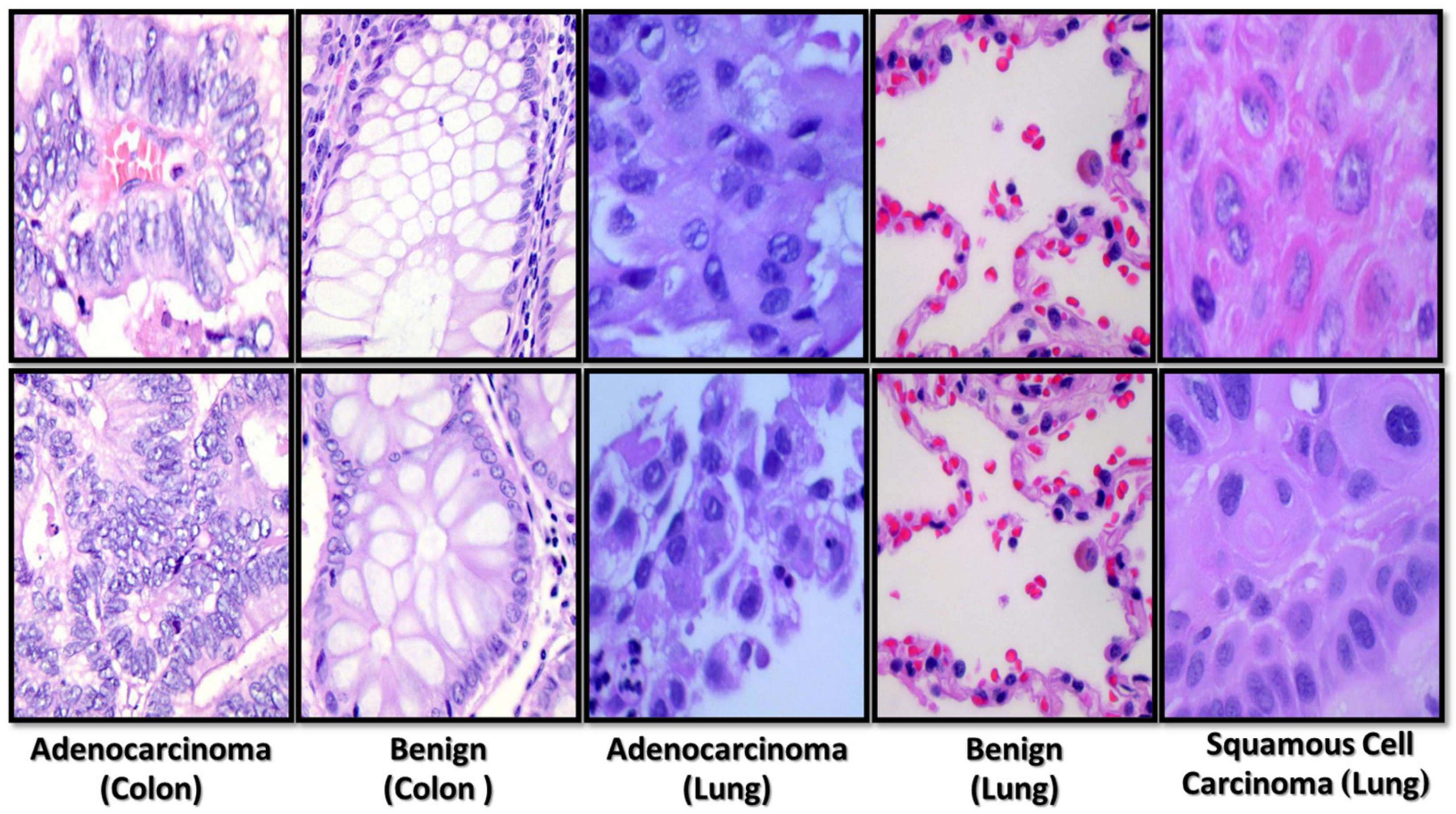
3.1. Dataset
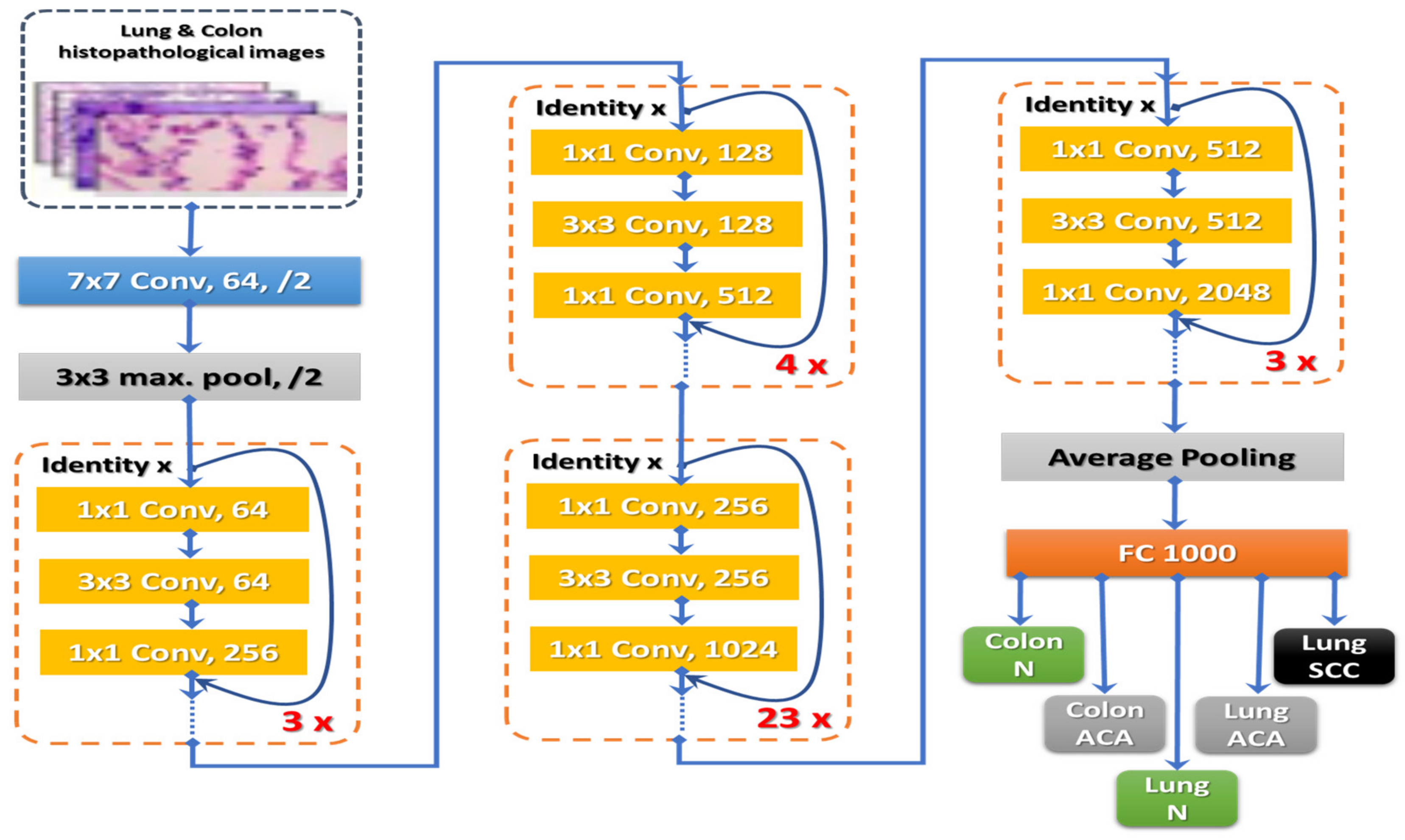
3.2. Model Architecture and Training
3.2.1. Prior Processing
3.2.2. Training Procedure
3.2.3. Optimization of the Network
Batch Normalization and Hyper-Parameter Tuning
Activation Function
Optimization
4. Model Implementation and Evaluation
4.1. Hardware and Software Specifications
4.2. Model Implementation
4.3. Performance Evaluation
4.4. Experimental Results
4.4.1. Analysis of ResNet101 Model
4.4.2. Comparison with Other Four Powerful Deep Learning Models
4.4.3. Comparison of the Proposed Model and the State-of-Art Methods
4.4.4. Discussion
5. Conclusions
Author Contributions
Funding
Institutional Review Board Statement
Informed Consent Statement
Data Availability Statement
Acknowledgments
Conflicts of Interest
References
- Cancer Country Profile. 2020. Available online: https://gco.iarc.fr/today/online-analysis-pie?v=2020&mode=cancer&mode_population=continents&population=900&populations=900&key=total&sex=0&cancer=39&type=1&statistic=5&prevalence=0&population_group=0&ages_group%5B%5D=0&ages_group%5B%5D=17&nb_items=7&group_cancer=1&include_nmsc=1&include_nmsc_other=1&half_pie=0&donut=0 (accessed on 17 November 2022).
- Cancer Facts & Figures 2022. Available online: https://www.cancer.org/research/cancer-facts-statistics/all-cancer-facts-figures/cancer-facts-figures-2022.html (accessed on 17 November 2022).
- Cancer. Available online: https://www.who.int/news-room/fact-sheets/detail/cancer (accessed on 30 August 2022).
- Cancer—Symptoms and Causes—Mayo Clinic. Available online: https://www.mayoclinic.org/diseases-conditions/cancer/symptoms-causes/syc-20370588 (accessed on 30 August 2022).
- Daye, D.; Tabari, A.; Kim, H.; Chang, K.; Kamran, S.C.; Hong, T.S.; Kalpathy-Cramer, J.; Gee, M.S. Quantitative tumor heterogeneity MRI profiling improves machine learning-based prognostication in patients with metastatic colon cancer. Eur. Radiol. 2021, 31, 5759–5767. [Google Scholar] [CrossRef] [PubMed]
- Bębas, E.; Borowska, M.; Derlatka, M.; Oczeretko, E.; Hładuński, M.; Szumowski, P.; Mojsak, M. Machine-learning-based classification of the histological subtype of non-small-cell lung cancer using MRI texture analysis. Biomed. Signal Process. Control 2021, 66, 102446. [Google Scholar] [CrossRef]
- Comes, M.C.; Fanizzi, A.; Bove, S.; Didonna, V.; Diotaiuti, S.; La Forgia, D.; Latorre, A.; Martinelli, E.; Mencattini, A.; Nardone, A.; et al. Early prediction of neoadjuvant chemotherapy response by exploiting a transfer learning approach on breast DCE-MRIs. Sci. Rep. 2021, 11, 14123. [Google Scholar] [CrossRef]
- Comes, M.C.; La Forgia, D.; Didonna, V.; Fanizzi, A.; Giotta, F.; Latorre, A.; Martinelli, E.; Mencattini, A.; Paradiso, A.V.; Tamborra, P.; et al. Early Prediction of Breast Cancer Recurrence for Patients Treated with Neoadjuvant Chemotherapy: A Transfer Learning Approach on DCE-MRIs. Cancers 2021, 13, 2298. [Google Scholar] [CrossRef] [PubMed]
- Ali, M.; Ali, R. Multi-Input Dual-Stream Capsule Network for Improved Lung and Colon Cancer Classification. Diagnostics 2021, 11, 1485. [Google Scholar] [CrossRef] [PubMed]
- Shen, D.; Wu, G.; Suk, H.I. Deep learning in medical image analysis. Annu. Rev. Biomed. Eng. 2017, 19, 221–248. [Google Scholar] [CrossRef]
- Cai, L.; Gao, J.; Zhao, D. A review of the application of deep learning in medical image classification and segmentation. Ann. Transl. Med. 2020, 8, 713. [Google Scholar] [CrossRef]
- Haskins, G.; Kruger, U.; Yan, P. Deep learning in medical image registration: A survey. Mach. Vis. Appl. 2020, 31, 1–18. [Google Scholar]
- Wang, S.; Yang, D.M.; Rong, R.; Zhan, X.; Fujimoto, J.; Liu, H.; Minna, J.; Wistuba, I.I.; Xie, Y.; Xiao, G. Artificial intelligence in lung cancer pathology image analysis. Cancers 2019, 11, 1673. [Google Scholar] [CrossRef]
- Houssami, N.; Kirkpatrick-Jones, G.; Noguchi, N.; Lee, C.I. Artificial Intelligence (AI) for the early detection of breast cancer: A scoping review to assess AI’s potential in breast screening practice. Expert Rev. Med. Devices 2019, 16, 351–362. [Google Scholar] [CrossRef]
- Rakhlin, A.; Shvets, A.; Iglovikov, V.; Kalinin, A.A. Deep convolutional neural networks for breast cancer histology image analysis. In International Conference Image Analysis and Recognition; Springer: Berlin/Heidelberg, Germany, 2018; pp. 737–744. [Google Scholar]
- Lorencin, I.; Anđelić, N.; Španjol, J.; Car, Z. Using multi-layer perceptron with Laplacian edge detector for bladder cancer diagnosis. Artif. Intell. Med. 2020, 102, 101746. [Google Scholar] [CrossRef] [PubMed]
- Lorencin, I.; Anđelić, N.; Šegota, S.B.; Musulin, J.; Štifanić, D.; Mrzljak, V.; Španjol, J.; Car, Z. Edge detector-based hybrid artificial neural network models for urinary bladder cancer diagnosis. In Enabling AI Applications in Data Science; Springer: Berlin/Heidelberg, Germany, 2021; pp. 225–245. [Google Scholar]
- Jinnai, S.; Yamazaki, N.; Hirano, Y.; Sugawara, Y.; Ohe, Y.; Hamamoto, R. The development of a skin cancer classification system for pigmented skin lesions using deep learning. Biomolecules 2020, 10, 1123. [Google Scholar] [CrossRef] [PubMed]
- Aida, S.; Okugawa, J.; Fujisaka, S.; Kasai, T.; Kameda, H.; Sugiyama, T. Deep Learning of Cancer Stem Cell Morphology Using Conditional Generative Adversarial Networks. Biomolecules 2020, 10, 931. [Google Scholar] [CrossRef] [PubMed]
- Yoon, H.J.; Kim, S.; Kim, J.H.; Keum, J.S.; Oh, S.I.; Jo, J.; Chun, J.; Youn, Y.H.; Park, H.; Kwon, I.G.; et al. A lesion-based convolutional neural network improves endoscopic detection and depth prediction of early gastric cancer. J. Clin. Med. 2019, 8, 1310. [Google Scholar] [CrossRef] [PubMed]
- Musulin, J.; Štifanić, D.; Zulijani, A.; Ćabov, T.; Dekanić, A.; Car, Z. An enhanced histopathology analysis: An AI-Based System for Multiclass Grading of Oral Squamous Cell Carcinoma and Segmenting of Epithelial and Stromal Tissue. Cancers 2021, 13, 1784. [Google Scholar] [CrossRef] [PubMed]
- Pereira, T.; Freitas, C.; Costa, J.L.; Morgado, J.; Silva, F.; Negrão, E.; de Lima, B.F.; da Silva, M.C.; Madureira, A.J.; Ramos, I.; et al. Comprehensive Perspective for Lung Cancer Characterisation Based on AI Solutions Using CT Images. J. Clin. Med. 2021, 10, 118. [Google Scholar] [CrossRef] [PubMed]
- Hägele, M.; Seegerer, P.; Lapuschkin, S.; Bockmayr, M.; Samek, W.; Klauschen, F.; Müller, K.R.; Binder, A. Resolving challenges in deep learning-based analyses of histopathological images using explanation methods. Sci. Rep. 2020, 10, 1–12. [Google Scholar] [CrossRef]
- van der Laak, J.; Litjens, G.; Ciompi, F. Deep learning in histopathology: The path to the clinic. Nat. Med. 2021, 27, 775–784. [Google Scholar] [CrossRef]
- Sakr, A.S.; Soliman, N.F.; Al-Gaashani, M.S.; Pławiak, P.; Ateya, A.A.; Hammad, M. An Efficient Deep Learning Approach for Colon Cancer Detection. Appl. Sci. 2022, 12, 8450. [Google Scholar] [CrossRef]
- Nishio, M.; Nishio, M.; Jimbo, N.; Nakane, K. Homology-Based Image Processing for Automatic Classification of Histopathological Images of Lung Tissue. Cancers 2021, 13, 1192. [Google Scholar] [CrossRef]
- Masud, M.; Sikder, N.; Nahid, A.A.; Bairagi, A.K.; AlZain, M.A. A machine learning approach to diagnosing lung and colon cancer using a deep learning-based classification framework. Sensors 2021, 21, 748. [Google Scholar] [CrossRef] [PubMed]
- Pacal, I.; Karaboga, D.; Basturk, A.; Akay, B.; Nalbantoglu, U. A comprehensive review of deep learning in colon cancer. Comput. Biol. Med. 2020, 126, 104003. [Google Scholar] [CrossRef] [PubMed]
- Debelee, T.G.; Kebede, S.R.; Schwenker, F.; Shewarega, Z.M. Deep learning in selected cancers’ image analysis—A survey. J. Imaging 2020, 6, 121. [Google Scholar] [CrossRef] [PubMed]
- Abbas, M.A.; Bukhari, S.U.K.; Syed, A.; Shah, S.S.H. The Histopathological Diagnosis of Adenocarcinoma & Squamous Cells Carcinoma of Lungs by Artificial intelligence: A comparative study of convolutional neural networks. medRxiv 2020. [Google Scholar] [CrossRef]
- Roy Medhi, B.B. Lung Cancer Classification from Histologic Images Using Capsule Networks. Ph.D. Thesis, National College of Ireland, Dublin, Ireland, 2020. [Google Scholar]
- Bukhari, S.U.K.; Asmara, S.; Bokhari, S.K.A.; Hussain, S.S.; Armaghan, S.U.; Shah, S.S.H. The Histological Diagnosis of Colonic Adenocarcinoma by Applying Partial Self Supervised Learning. medRxiv 2020. [Google Scholar] [CrossRef]
- Suresh, S.; Mohan, S. ROI-based feature learning for efficient true positive prediction using convolutional neural network for lung cancer diagnosis. Neural Comput. Appl. 2020, 32, 15989–16009. [Google Scholar] [CrossRef]
- Masud, M.; Muhammad, G.; Hossain, M.S.; Alhumyani, H.; Alshamrani, S.; Cheikhrouhou, O.; Ibrahim, S. Light Deep Model for Pulmonary Nodule Detection from CT Scan Images for Mobile Devices. Wirel. Commun. Mob. Comput. 2020, 2020, 8893494. [Google Scholar] [CrossRef]
- Shakeel, P.M.; Burhanuddin, M.A.; Desa, M.I. Automatic lung cancer detection from CT image using improved deep neural network and ensemble classifier. Neural Comput. Appl. 2020, 34, 9579–9592. [Google Scholar] [CrossRef]
- Mangal, S.; Chaurasia, A.; Khajanchi, A. Convolution Neural Networks for diagnosing colon and lung cancer histopathological images. arXiv 2020, arXiv:2009.03878. [Google Scholar]
- Borkowski, A.A.; Bui, M.M.; Thomas, L.B.; Wilson, C.P.; DeLand, L.A.; Mastorides, S.M. Lung and Colon Cancer Histopathological Image Dataset (LC25000). arXiv 2019, arXiv:1912.12142. [Google Scholar]
- Brinker, T.J.; Hekler, A.; Enk, A.H.; von Kalle, C. Enhanced classifier training to improve precision of a convolutional neural network to identify images of skin lesions. PLoS ONE 2019, 14, e0218713. [Google Scholar] [CrossRef] [PubMed]
- Hanif, M.S.; Bilal, M. Competitive residual neural network for image classification. ICT Express 2020, 6, 28–37. [Google Scholar] [CrossRef]
- He, K.; Zhang, X.; Ren, S.; Sun, J. Deep Residual Learning for Image Recognition. In Proceedings of the 2016 IEEE Conference on Computer Vision and Pattern Recognition (CVPR), Las Vegas, NV, USA, 27–30 June 2016. [Google Scholar]
- Theckedath, D.; Sedamkar, R.R. Detecting Affect States Using VGG16, ResNet50 and SE-ResNet50 Networks. SN Comput. Sci. 2020, 1, 79. [Google Scholar] [CrossRef]
- Zouggar, S.T.; Adla, A. Optimization Techniques for Machine Learning. In Algorithms for Intelligent Systems; Springer: Singapore, 2019; pp. 31–50. [Google Scholar] [CrossRef]
- Bottou, L.; Curtis, F.E.; Nocedal, J. Optimization Methods for Large-Scale Machine Learning. SIAM Rev. 2018, 60, 223–311. [Google Scholar] [CrossRef]
- Dogo, E.M.; Afolabi, O.J.; Nwulu, N.I.; Twala, B.; Aigbavboa, C.O. A Comparative Analysis of Gradient Descent-Based Optimization Algorithms on Convolutional Neural Networks. In Proceedings of the 2018 International Conference on Computational Techniques, Electronics and Mechanical Systems (CTEMS), Belgaum, India, 21–22 December 2018. [Google Scholar]
- Sun, S.; Cao, Z.; Zhu, H.; Zhao, J. A Survey of Optimization Methods From a Machine Learning Perspective. IEEE Trans. Cybern. 2020, 50, 3668–3681. [Google Scholar] [CrossRef]
- Yaseen, M.U.; Anjum, A.; Rana, O.; Antonopoulos, N. Deep Learning Hyper-Parameter Optimization for Video Analytics in Clouds. IEEE Trans. Syst. Man Cybern. Syst. 2019, 49, 253–264. [Google Scholar] [CrossRef]
- Mahbod, A.; Schaefer, G.; Wang, C.; Ecker, R.; Ellinge, I. Skin Lesion Classification Using Hybrid Deep Neural Networks. In Proceedings of the ICASSP 2019—2019 IEEE International Conference on Acoustics, Speech, and Signal Processing (ICASSP), Brighton, UK, 12–17 May 2019. [Google Scholar]
- Yin, Z.; Wan, B.; Yuan, F.; Xia, X.; Shi, J. A Deep Normalization and Convolutional Neural Network for Image Smoke Detection. IEEE Access 2017, 5, 18429–18438. [Google Scholar] [CrossRef]
- Pham, T.-C.; Doucet, A.; Luong, C.-M.; Tran, C.-T.; Hoang, V.-D. Improving Skin-Disease Classification Based on Customized Loss Function Combined With Balanced Mini-Batch Logic and Real-Time Image Augmentation. IEEE Access 2020, 8, 150725–150737. [Google Scholar] [CrossRef]
- Fu, Z.; Li, S.; Li, X.; Dan, B.; Wang, X. Influence of Batch Normalization on Convolutional Neural Networks in HRRP Target Recognition. In Proceedings of the 2019 International Applied Computational Electromagnetics Society Symposium—China (ACES), Nanjing, China, 8–11 August 2019. [Google Scholar]
- Goceri, E. Analysis of Deep Networks with Residual Blocks and Different Activation Functions: Classification of Skin Diseases. In Proceedings of the 2019 Ninth International Conference on Image Processing Theory, Tools and Applications (IPTA), Istanbul, Turkey, 6–9 November 2019. [Google Scholar]
- Altaf, F.; Islam, S.M.S.; Akhtar, N.; Janjua, N.K. Going Deep in Medical Image Analysis: Concepts, Methods, Challenges, and Future Directions. IEEE Access 2019, 7, 99540–99572. [Google Scholar] [CrossRef]
- Kirana, K.C.; Wibawanto, S.; Hidayah, N.; Cahyono, G.P.; Asfani, K. Improved Neural Network using Integral-RELU based Prevention Activation for Face Detection. In Proceedings of the 2019 International Conference on Electrical, Electronics and Information Engineering (ICEEIE), Denpasar, Indonesia, 3–4 October 2019. [Google Scholar]
- Yamashita, R.; Nishio, M.; Do, R.K.G.; Togashi, K. Convolutional neural networks: An overview and application in radiology. Insights Into Imaging 2018, 9, 611–629. [Google Scholar] [CrossRef]
- Adegun, A.A.; Viriri, S. Deep Learning-Based System for Automatic Melanoma Detection. IEEE Access 2020, 8, 7160–7172. [Google Scholar] [CrossRef]
- Vipin, V.; Nath, M.K.; Sreejith, V.; Giji, N.F.; Ramesh, A.; Meera, M. Detection of Melanoma using Deep Learning Techniques. In Proceedings of the 2020 International Conference on Computation, Automation and Knowledge Management (ICCAKM), Idukki, India, 16–18 June 2021. [Google Scholar]
- Koshy, R.; Mahmood, A. Optimizing Deep CNN Architectures for Face Liveness Detection. Entropy 2019, 21, 423. [Google Scholar] [CrossRef] [PubMed]


| Study | Methodology | Obtained Results | Dataset | Limitation |
|---|---|---|---|---|
| Sakr et al. [25] | CNN with four convolution block | Accuracy = 99.5% | LC25000 | Only colon cancer |
| Masud et al. [27] | Multi-channel CNN | Accuracy = 96.33% | LC25000 | Custom architecture |
| Mangal et al. [36] | Multi-channel CNN | Accuracy = 97.89% | LC25000 | |
| Abbas et al. [30] | VGG-19, Alex Net, ResNet: ResNet-18, ResNet-34, ResNet-50, and ResNet-101 | F-1 scores = 0.973, 0.997, 0.986, 0.992, 0.999, and 0.999, respectively | LC25000 | Only lung cancer |
| Roy Medhi [31] | Capsule network | Accuracy = 99% | LC25000 | Only lung cancer |
| Bukhari et al. [32] | ResNet-18, ResNet-30, and ResNet50 | ResNet-50 accuracy = 93.91% ResNet-30 accuracy = 93.04% ResNet-18 accuracy = 93.04% | LC25000 | Only colon cancer |
| Hyper-Parameters | Value | The Best Value |
|---|---|---|
| Number of epochs | 14 | 14 |
| Batch size | 40/80 | 80 |
| Activation function | Swish/ReLU | ReLU |
| Optimizer | Adam/AdaMax/SGD | AdaMax |
| Initial learning rate | 0.001 | 0.001 |
| Dropout | 0.5 | 0.5 |
| Patience | 10 | 10 |
| Loss function | Categorical cross-entropy | Categorical cross-entropy |
| Batch | Parameters | Precision (%) | Recall (%) | F-Score (%) | Specificity (%) | Accuracy (%) | Cohen Kappa (%) | Test_Time/Step |
|---|---|---|---|---|---|---|---|---|
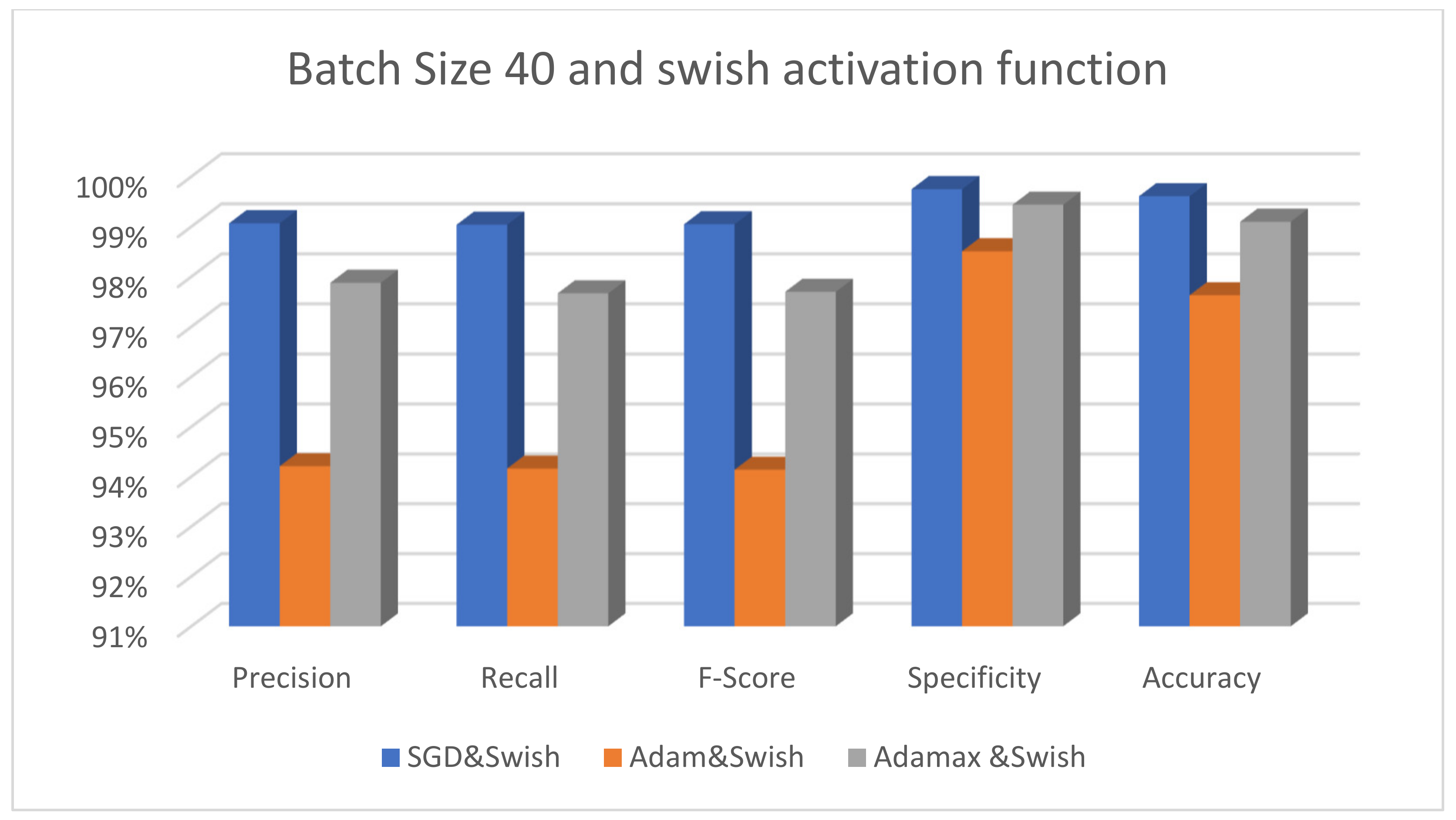
| Batch size 40 | SGD&Swish | 99.07 | 99.04 | 99.05 | 99.75 | 99.61 | 98.39 | 5 s 215 ms |
| Adam&Swish | 94.21 | 94.16 | 94.14 | 98.51 | 97.63 | 91.99 | 7 s 213 ms | |
| Adamax&Swish | 97.88 | 97.67 | 97.70 | 99.44 | 99.10 | 96.40 | 7 s 213 ms | |
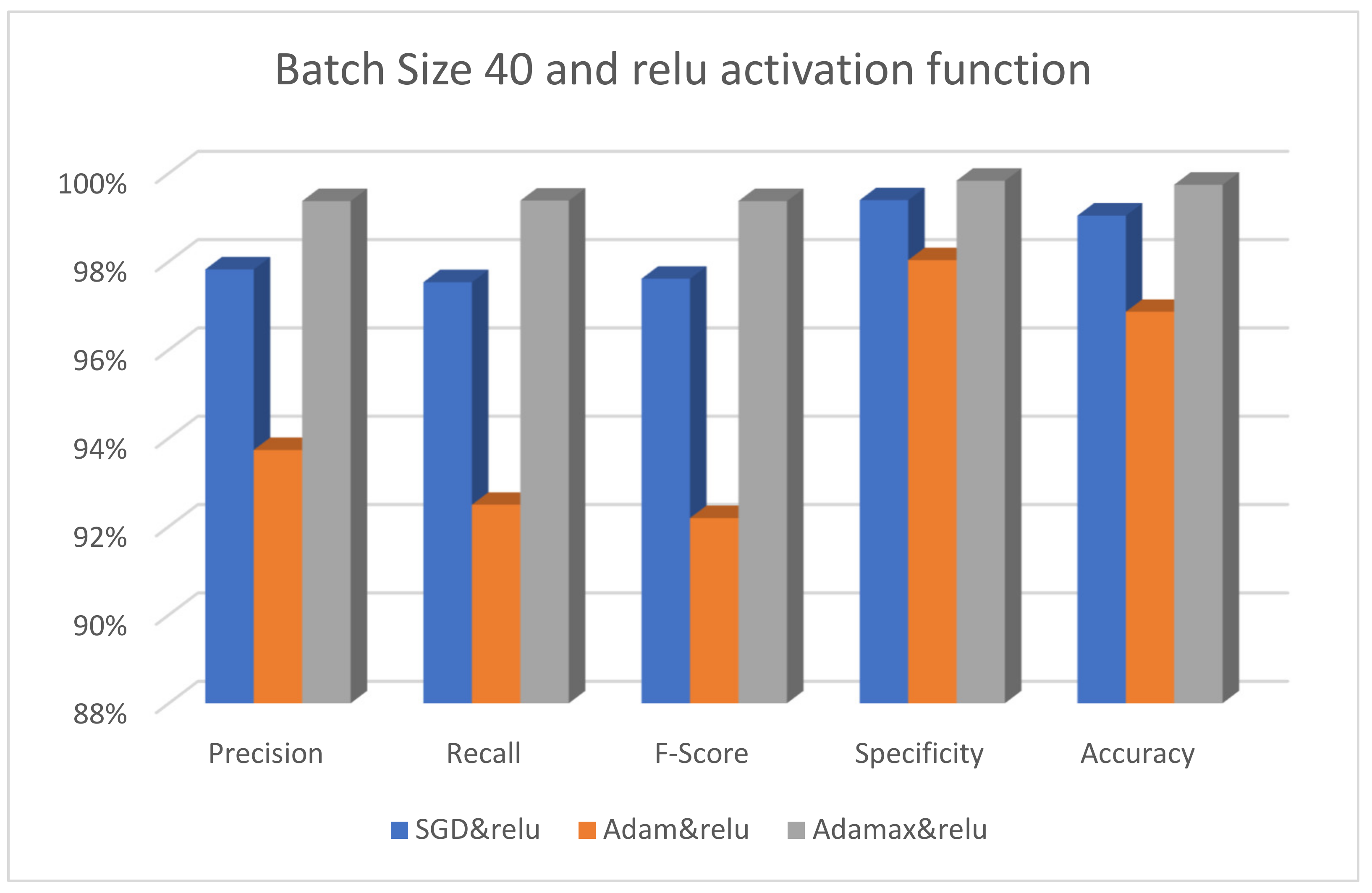
| SGD&ReLU | 97.82 | 97.53 | 97.61 | 99.39 | 99.04 | 96.00 | 8 s 239 ms | |
| Adam&ReLU | 93.73 | 92.49 | 92.19 | 98.03 | 96.86 | 89.24 | 8 s 244 ms | |
| Adamax&ReLU | 99.37 | 99.38 | 99.37 | 99.83 | 99.74 | 100.00 | 7 s 227 ms | |
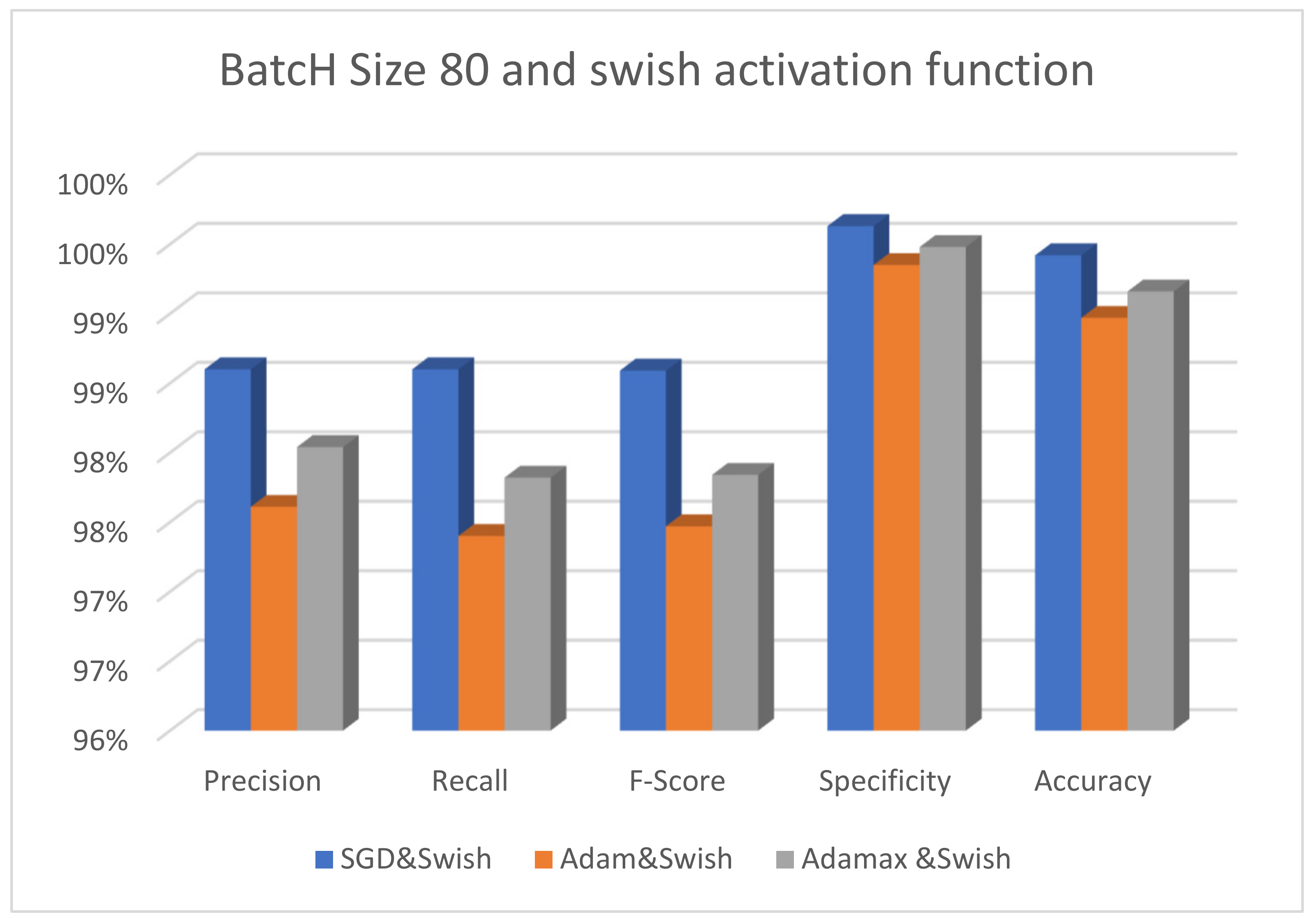
| Batch size 80 | SGD&Swish | 98.60 | 98.60 | 98.59 | 99.63 | 99.42 | 97.60 | 5 s 198 ms |
| Adam&Swish | 97.61 | 97.40 | 97.47 | 99.35 | 98.97 | 97.20 | 7 s 232 ms | |
| Adamax&Swish | 98.04 | 97.82 | 97.84 | 99.48 | 99.16 | 97.20 | 7 s 219 ms | |
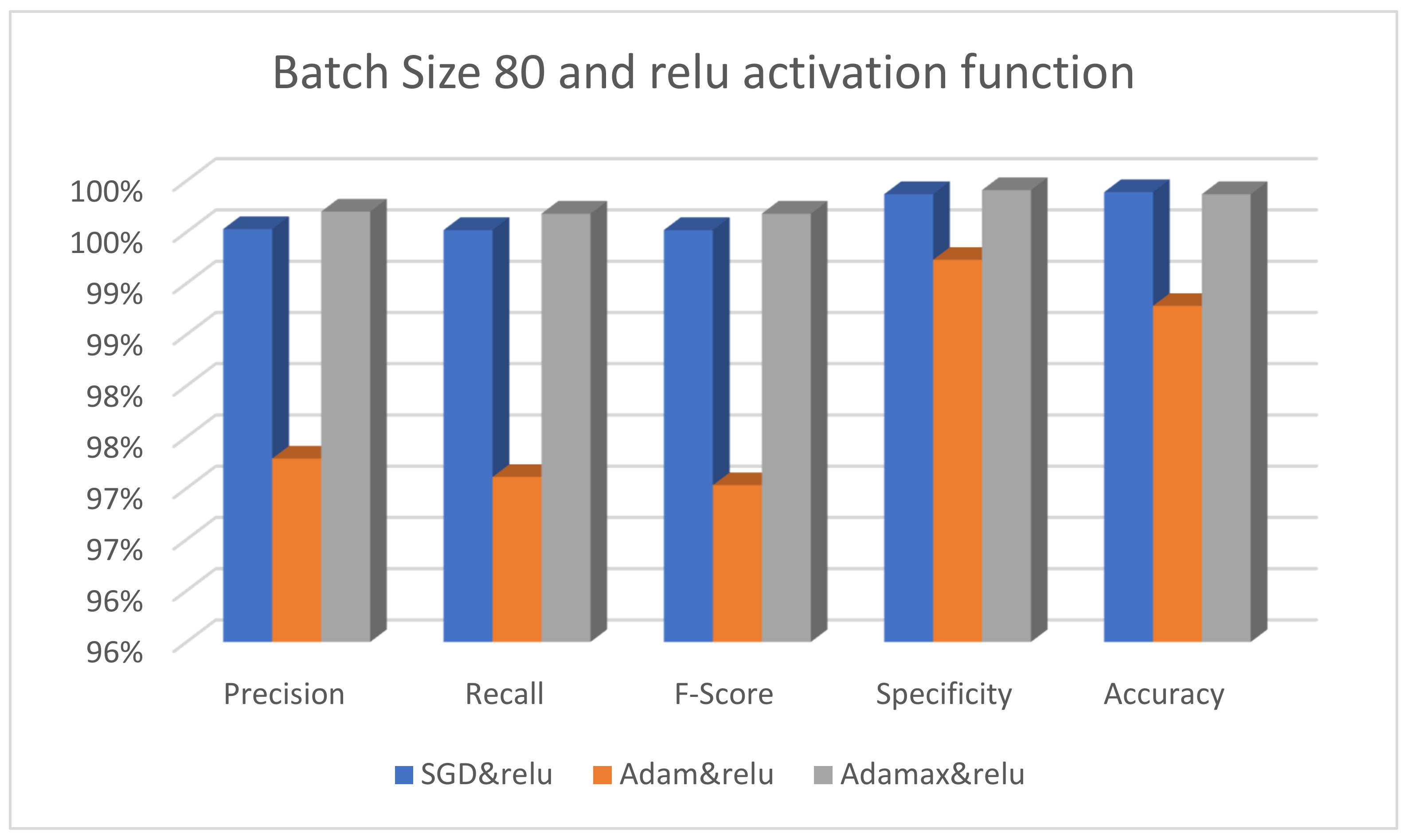
| SGD&ReLU | 99.53 | 99.52 | 99.52 | 99.87 | 99.89 | 99.60 | 7 s 224 ms | |
| Adam&ReLU | 97.29 | 97.11 | 97.03 | 99.23 | 98.78 | 98.00 | 7 s 217 ms | |
| Adamax&ReLU | 99.70 | 99.68 | 99.68 | 99.91 | 99.87 | 99.60 | 6 s 232 ms |
| Precision (%) | Recall (%) | F1-Score (%) | Specificity (%) | Accuracy (%) | |
|---|---|---|---|---|---|
| MobileNet | 99.52 | 99.52 | 99.52 | 99.88 | 99.81 |
| Xception | 99.61 | 99.20 | 99.60 | 99.60 | 99.84 |
| VGG16 | 94.22 | 94.08 | 94.06 | 98.52 | 97.63 |
| InceptionV3 | 99.60 | 99.60 | 99.60 | 99.90 | 99.84 |
| Resnet101 | 99.84 | 99.85 | 99.84 | 99.96 | 99.94 |
| Reference | Methodology | Performance |
|---|---|---|
| Bukhari et al. [30] | ResNet-18, ResNet-30, and ResNet-50 | ResNet-50 accuracy = 93.91% ResNet-30 accuracy = 93.04% ResNet-18 accuracy = 93.04% |
| Roy Medhi [29] | Capsule network | Accuracy = 99% |
| Abbas et al. [28] | VGG-19, Alex Net, ResNet: ResNet-18, ResNet-34, ResNet-50, and ResNet-101 | F-1 scores = 0.973, 0.997, 0.986, 0.992, 0.999, and 0.999, respectively |
| Sakr et al. [36] | CNN with four convolution block | Accuracy = 99.5% |
| Masud et al. [25] | Multi-channel CNN | Accuracy = 96.33% |
| Mangal et al. [34] | Multi-channel CNN | Accuracy = 97.89% |
| The proposed model | Fine-tuned ResNet101 | Precision (99.84%), recall (99.85%), F-Score (99.84%), specificity (99.96%), and accuracy (99.94) |
Disclaimer/Publisher’s Note: The statements, opinions and data contained in all publications are solely those of the individual author(s) and contributor(s) and not of MDPI and/or the editor(s). MDPI and/or the editor(s) disclaim responsibility for any injury to people or property resulting from any ideas, methods, instructions or products referred to in the content. |
© 2023 by the authors. Licensee MDPI, Basel, Switzerland. This article is an open access article distributed under the terms and conditions of the Creative Commons Attribution (CC BY) license (https://creativecommons.org/licenses/by/4.0/).
Share and Cite
El-Ghany, S.A.; Azad, M.; Elmogy, M. Robustness Fine-Tuning Deep Learning Model for Cancers Diagnosis Based on Histopathology Image Analysis. Diagnostics 2023, 13, 699. https://doi.org/10.3390/diagnostics13040699
El-Ghany SA, Azad M, Elmogy M. Robustness Fine-Tuning Deep Learning Model for Cancers Diagnosis Based on Histopathology Image Analysis. Diagnostics. 2023; 13(4):699. https://doi.org/10.3390/diagnostics13040699
Chicago/Turabian StyleEl-Ghany, Sameh Abd, Mohammad Azad, and Mohammed Elmogy. 2023. "Robustness Fine-Tuning Deep Learning Model for Cancers Diagnosis Based on Histopathology Image Analysis" Diagnostics 13, no. 4: 699. https://doi.org/10.3390/diagnostics13040699