
NanoChest-Net: A Simple Convolutional Network for Radiological Studies Classification

 ,
,  , ,
, ,
Abstract
:1. Introduction
2. Materials and Methods
2.1. Datasets
2.1.1. Tuberculosis Dataset
2.1.2. Pneumonia Children Dataset
2.1.3. COVID-19 Dataset
2.1.4. RSNA Pneumonia Challenge Dataset
2.1.5. BCDR Dataset
2.2. CNN Models from the State of the Art
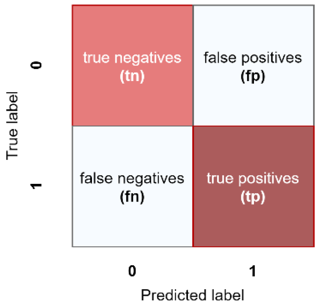
2.3. Metrics
3. Proposal
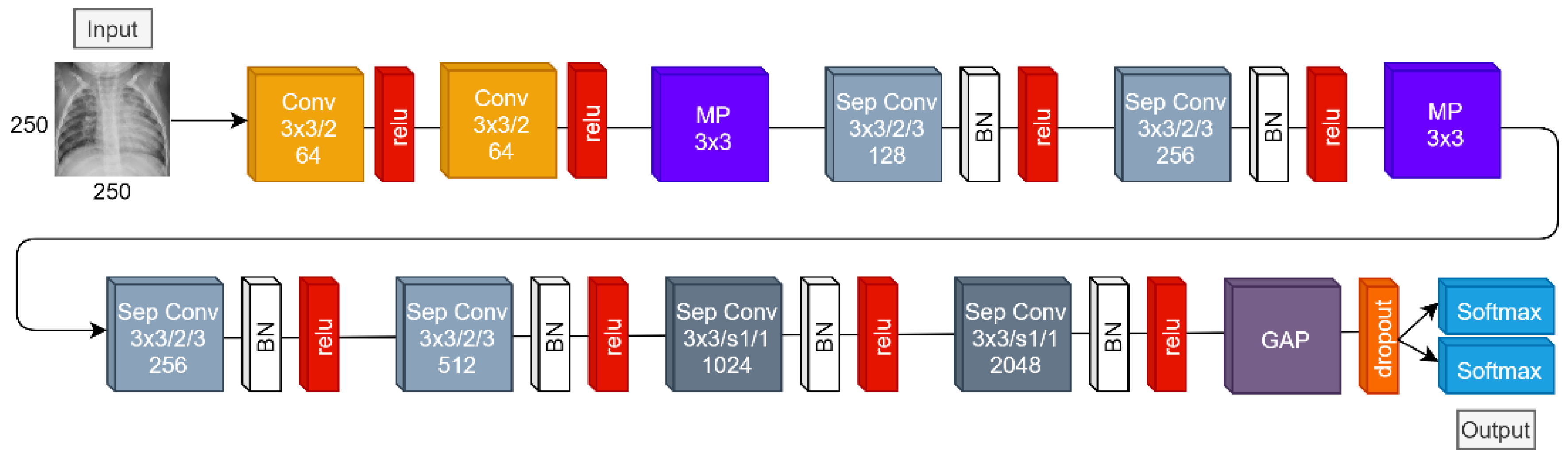
3.1. DL Model
3.2. Datasets Splitting and Validation Method
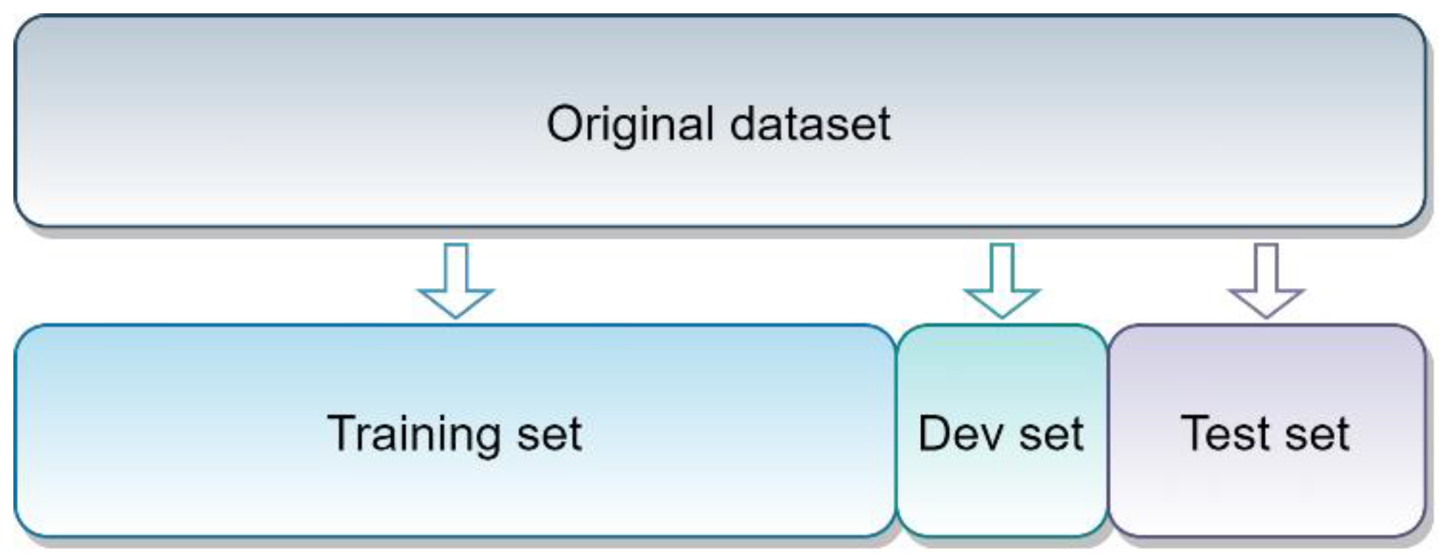
3.2.1. Splitting and Final Datasets
3.2.2. Validation Method
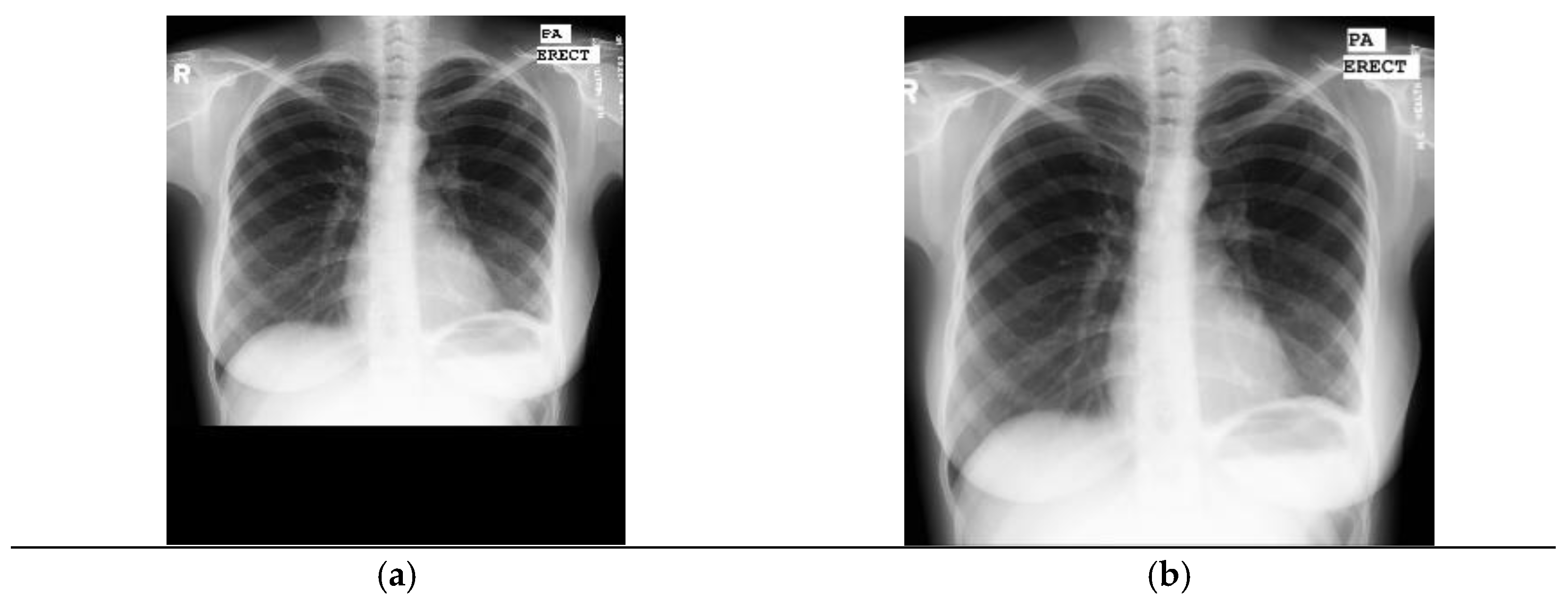
3.3. Preprocessing and Data Augmentation
Tuberculosis Montgomery County Dataset
3.4. Hyperparameter Tuning
4. Results
4.1. Experimental Framework
4.2. Test Sets Results
4.3. Training Time Results
4.4. Size of the Models
4.5. Statistical Analysis
5. Discussion
6. Conclusions
Author Contributions
Funding
Institutional Review Board Statement
Informed Consent Statement
Data Availability Statement
Acknowledgments
Conflicts of Interest
References
- World Health Organization. Coronavirus Disease (COVID-19) Pandemic. 2020. Available online: https://www.who.int/emergencies/diseases/novel-coronavirus-2019 (accessed on 24 April 2021).
- World Health Organization. Pneumonia. 2019. Available online: https://www.who.int/news-room/fact-sheets/detail/pneumonia (accessed on 12 March 2021).
- World Health Organization. Tuberculosis. 2020. Available online: https://www.who.int/westernpacific/health-topics/tuberculosis (accessed on 12 March 2021).
- World Cancer Research Fund. Breast Cancer Statistics. 2018. Available online: https://www.wcrf.org/dietandcancer/cancer-trends/breast-cancer-statistics (accessed on 12 March 2021).
- Suetens, P. Fundamentals of Medical Imaging, 2nd ed.; Cambridge University Press: New York, NY, USA, 2009. [Google Scholar]
- Sutton, D. Textbook of Radiology and Imaging, 7th ed.; Chirchill Livingstone: London, UK, 2003. [Google Scholar]
- Goodman, L.R. Felson’s Principles of Chest Roentgenology: A Programmed Text, 3rd ed.; Saunders: Philadelphia, PA, USA, 2007. [Google Scholar]
- Fauci, K.; Longo, H.; Loscalzo, J. Harrison’s Principles of Internal Medicine, 19th ed.; McGraw-Hill Education: New York, NY, USA, 2015. [Google Scholar]
- Doi, K. Computer-Aided Diagnosis in Medical Imaging: Historical Review, Current Status and Future Poten-tial. Computerized medical imaging and graphics. Off. J. Comput. Med. Imaging Soc. 2007, 31, 198–211. [Google Scholar] [CrossRef] [Green Version]
- Livieris, I.E.; Kanavos, A.; Tampakas, V.; Pintelas, P. An Ensemble SSL Algorithm for Efficient Chest X-Ray Image Classification. J. Imaging 2018, 4, 95. [Google Scholar] [CrossRef] [Green Version]
- Minaee, S.; Wang, Y.; Lui, Y.W. Prediction of Longterm Outcome of Neuropsychological Tests of MTBI Patients Using Imaging Features. In Proceedings of the 2013 IEEE Signal Processing in Medicine and Biology Symposium (SPMB), Brooklyn, NY, USA, 7 December 2013. [Google Scholar]
- Chan, H.; Hadjiiski, L.M.; Samala, R.K. Computer-aided diagnosis in the era of deep learning. Med. Phys. 2020, 47, e218–e227. [Google Scholar] [CrossRef] [PubMed]
- Pathan, S.; Kumar, P.; Pai, R.M.; Bhandary, S.V. Automated segmentation and classifcation of retinal features for glaucoma diagnosis. Biomed. Signal Process. Control 2021, 63, 102244. [Google Scholar] [CrossRef]
- Oulefki, A.; Agaian, S.; Trongtirakul, T.; Laouar, A.K. Automatic COVID-19 lung infected region segmentation and measurement using CT-scans images. Pattern Recognit. 2021, 114, 107747. [Google Scholar] [CrossRef] [PubMed]
- Qiu, Y.; Liu, Y.; Li, S.; Xu, J. MiniSeg: An Extremely Minimum Network for Efficient COVID-19 Segmentation. arXiv 2021, arXiv:2004.09750. [Google Scholar]
- Gautam, A.; Raman, B. Towards effective classification of brain hemorrhagic and ischemic stroke using CNN. Biomed. Signal Process. Control 2021, 63, 102178. [Google Scholar] [CrossRef]
- Mbarki, W.; Bouchouicha, M.; Frizzi, S.; Tshibasu, F.; Ben Farhat, L.; Sayadi, M. Lumbar spine discs classification based on deep convolutional neural networks using axial view MRI. Interdiscip. Neurosurg. 2020, 22, 100837. [Google Scholar] [CrossRef]
- Martínez-Más, J.; Bueno-Crespo, A.; Martínez-España, R.; Remezal-Solano, M.; Ortiz-González, A.; Ortiz-Reina, S.; Martínez-Cendán, J.P. Classifying Papanicolaou cervical smears through a cell merger approach by deep learning technique. Expert Syst. Appl. 2020, 160, 113707. [Google Scholar] [CrossRef]
- Zhou, H.; Wang, K.; Tian, J. Online Transfer Learning for Differential Diagnosis of Benign and Malignant Thyroid Nodules with Ultrasound Images. IEEE Trans. Biomed. Eng. 2020, 67, 2773–2780. [Google Scholar] [CrossRef]
- Rajan, D.; Thiagarajan, J.J.; Karargyris, A.; Kashyap, S. Self-Training with Improved Regularization for Few-Shot Chest X-Ray Classification. arXiv 2020, arXiv:2005.02231. [Google Scholar]
- Sharma, S.; Ghose, S.; Datta, S.; Malathy, C.; Gayathri, M.; Prabhakaran, M. CORONA-19 NET: Transfer Learning Approach for Automatic Classification of Coronavirus Infections in Chest Radiographs. In Advances in Intelligent Systems and Computing; Springer International Publishing: New York, NY, USA, 2021; Volume 1200 AISC, pp. 526–534. [Google Scholar]
- Zebin, T.; Rezvy, S. COVID-19 detection and disease progression visualization: Deep learning on chest X-rays for classification and coarse localization. Appl. Intell. 2021, 51, 1010–1021. [Google Scholar] [CrossRef]
- Yu, Z.; Li, X.; Sun, H.; Wang, J.; Zhao, T.; Chen, H.; Ma, Y.; Zhu, S.; Xie, Z. Rapid identification of COVID-19 severity in CT scans through classification of deep features. Biomed. Eng. Online 2020, 19, 1–13. [Google Scholar] [CrossRef] [PubMed]
- Luján-García, J.E.; Moreno-Ibarra, M.A.; Villuendas-Rey, Y.; Yáñez-Márquez, C. Fast COVID-19 and Pneumonia Classification Using Chest X-ray Images. Mathematics 2020, 8, 1423. [Google Scholar] [CrossRef]
- Yazdani, S.; Minaee, S.; Kafieh, R.; Saeedizadeh, N.; Sonka, M. COVID CT-Net: Predicting Covid-19 from Chest CT Images Using Attentional Convolutional Network. arXiv 2020, arXiv:2009.05096. [Google Scholar]
- Gupta, A.; Anjum; Gupta, S.; Katarya, R. InstaCovNet-19: A deep learning classification model for the detection of COVID-19 patients using Chest X-ray. Appl. Soft Comput. 2020, 99, 106859. [Google Scholar] [CrossRef]
- Zhang, J.; Xie, Y.; Liao, Z.; Pang, G.; Verjans, J.; Li, W.; Sun, Z.; He, J.; Li, Y.; Shen, C.; et al. Viral Pneumonia Screening on Chest X-Ray Images Using Confidence-Aware Anomaly Detection. arXiv 2020, arXiv:2003.12338. [Google Scholar]
- Rahman, T.; Chowdhury, M.E.H.; Khandakar, A.; Islam, K.R.; Mahbub, Z.B.; Kadir, M.A.; Kashem, S. Transfer Learning with Deep Convolutional Neural Network (CNN) for Pneumonia Detection Using Chest X-ray. Appl. Sci. 2020, 10, 3233. [Google Scholar] [CrossRef]
- Luján-García, J.E.; Yáñez-Márquez, C.; Villuendas-Rey, Y.; Camacho-Nieto, O. A Transfer Learning Method for Pneumonia Classification and Visualization. Appl. Sci. 2020, 10, 2908. [Google Scholar] [CrossRef] [Green Version]
- Rajpurkar, P.; O’Connell, C.; Schechter, A.; Asnani, N.; Li, J.; Kiani, A.; Ball, R.L.; Mendelson, M.; Maartens, G.; Van Hoving, D.J.; et al. CheXaid: Deep learning assistance for physician diagnosis of tuberculosis using chest x-rays in patients with HIV. npj Digit. Med. 2020, 3, 1–8. [Google Scholar] [CrossRef]
- Pasa, F.; Golkov, V.; Pfeiffer, F.; Cremers, D. Efficient Deep Network Architectures for Fast Chest X-Ray Tuberculosis Screening and Visualization. Sci. Rep. 2019, 9, 1–9. [Google Scholar] [CrossRef] [PubMed] [Green Version]
- Khatibi, T.; Shahsavari, A.; Farahani, A. Proposing a novel multi-instance learning model for tuberculosis recognition from chest X-ray images based on CNNs, complex networks and stacked ensemble. Phys. Eng. Sci. Med. 2021, 44, 291–311. [Google Scholar] [CrossRef]
- Shen, L.; Margolies, L.R.; Rothstein, J.H.; Fluder, E.; McBride, R.; Sieh, W. Deep Learning to Improve Breast Cancer Detection on Screening Mammography. Sci. Rep. 2019, 9, 1–12. [Google Scholar] [CrossRef] [PubMed]
- Agarwal, R.; Diaz, O.; Lladó, X.; Yap, M.H.; Martí, R. Automatic mass detection in mammograms using deep convolutional neural networks. J. Med. Imaging 2019, 6, 31409. [Google Scholar] [CrossRef]
- Wu, N.; Phang, J.; Park, J.; Shen, Y.; Huang, Z.; Zorin, M.; Jastrzebski, S.; Fevry, T.; Katsnelson, J.; Kim, E.; et al. Deep Neural Networks Improve Radiologists’ Performance in Breast Cancer Screening. IEEE Trans. Med. Imaging 2020, 39, 1184–1194. [Google Scholar] [CrossRef] [Green Version]
- Jaeger, S.; Candemir, S.; Antani, S.; Wáng, Y.-X.J.; Lu, P.-X.; Thoma, G. Two public chest X-ray datasets for computer-aided screening of pulmonary diseases. Quant. Imaging Med. Surg. 2014, 4, 475–477. [Google Scholar]
- Kermany, D.; Zhang, K.; Goldbaum, M. Labeled Optical Coherence Tomography (OCT) and Chest X-Ray Images for Classification. Mendeley Data 2018. [Google Scholar] [CrossRef]
- Cohen, J.P.; Morrison, P.; Dao, L. COVID-19 Image Data Collection. arXiv 2020, arXiv:2003.11597. [Google Scholar]
- Moura, D.C.; Guevara López, M.A. An Evaluation of Image Descriptors Combined with Clinical Data for Breast Cancer Diagnosis. Int. J. Comput. Assist. Radiol. Surg. 2013, 8, 561–574. [Google Scholar] [CrossRef]
- LeCun, Y.; Bengio, Y.; Hinton, G. Deep learning. Nature 2015, 521, 436–444. [Google Scholar] [CrossRef]
- Kamil, M.Y. A deep learning framework to detect Covid-19 disease via chest X-ray and CT scan images. Int. J. Electr. Comput. Eng. IJECE 2021, 11, 844–850. [Google Scholar] [CrossRef]
- Chouhan, V.; Singh, S.K.; Khamparia, A.; Gupta, D.; Tiwari, P.; Moreira, C.; Damaševičius, R.; De Albuquerque, V.H.C. A Novel Transfer Learning Based Approach for Pneumonia Detection in Chest X-ray Images. Appl. Sci. 2020, 10, 559. [Google Scholar] [CrossRef] [Green Version]
- Liang, G.; Zheng, L. A transfer learning method with deep residual network for pediatric pneumonia diagnosis. Comput. Methods Progr. Biomed. 2020, 187, 104964. [Google Scholar] [CrossRef] [PubMed]
- He, K.; Zhang, X.; Ren, S.; Sun, J. Deep Residual Learning for Image Recognition. In Proceedings of the 2016 IEEE Conference on Computer Vision and Pattern Recognition (CVPR), Las Vegas, NV, USA, 27–30 June 2016; pp. 770–778. [Google Scholar]
- Chollet, F. Xception: Deep Learning with Depthwise Separable Convolutions. In Proceedings of the IEEE Conference on Computer Vision and Pattern Recognition (CVPR), Honolulu, HI, USA, 21–26 July 2017; pp. 125–1258. [Google Scholar]
- Huang, G.; Liu, Z.; van der Maaten, L.; Weinberger, K.Q. Densely Connected Convolutional Networks. In Proceedings of the IEEE Conference on Computer Vision and Pattern Recognition, Honolulu, HI, USA, 21–26 July 2017; pp. 4700–4708. [Google Scholar]
- Sokolova, M.; Lapalme, G. A systematic analysis of performance measures for classification tasks. Inf. Process. Manag. 2009, 45, 427–437. [Google Scholar] [CrossRef]
- Simonyan, K.; Zisserman, A. Very Deep Convolutional Networks for Large-Scale Image Recognition. In Proceedings of the International Conference on Learning Representations, Banff, AL, Canada, 14–16 April 2014. [Google Scholar]
- Kingma, D.P.; Ba, J. Adam: A method for stochastic optimization. In Proceedings of the International Conference Learn, Representations, San Diego, CA, USA, 5–8 May 2015. [Google Scholar]
- Sutskever, I.; Martens, J.; Dahl, G.; Hinton, G. On the Importance of Initialization and Momentum in Deep Learning. In Proceedings of the 30th International Conference on International Conference on Machine Learning, Atlanta, GA, USA, 16 June 2013; Volume 28, pp. III-1139–III-1147. [Google Scholar]
- Pedregosa, F.; Michel, V.; Grisel, O.; Blondel, M.; Prettenhofer, P.; Weiss, R.; Vanderplas, J.; Cournapeau, D.; Pedregosa, F.; Varoquaux, G.; et al. Scikit-Learn: Machine Learning in Python. J. Mach. Learn. Res. 2011, 12, 2825–2830. [Google Scholar]
- Bradski, G. The Open CV Library. Dr. Dobb’s J. Softw. Tools 2000, 120, 122–125. [Google Scholar]
- Friedman, M. The Use of Ranks to Avoid the Assumption of Normality Implicit in the Analysis of Variance. J. Am. Stat. Assoc. 1937, 32, 675. [Google Scholar] [CrossRef]
- Holm, S. A Simple Sequentially Rejective Multiple Test Procedure. Scand. J. Stat. 1979, 6, 65–70. [Google Scholar]


| Layer Type | Specifications |
|---|---|
| Input | Size = (250, 250, 3) |
| Convolution | Number of filters = 64 kernel size = (3, 3) dilatation rate = 2 padding = valid |
| Relu | Nonlinearity relu |
| Convolution | Number of filters = 64 kernel size = (3, 3) dilatation rate = 2 padding = valid |
| Relu | Nonlinearity relu |
| Max Pooling | Pool size = (3, 3) |
| Separable Convolution | Number of filters = 128 kernel size = (3, 3) dilatation rate = 2 depth multiplier = 3 padding = valid |
| Batch Normalization | Normalization |
| Relu | Nonlinearity relu |
| Separable Convolution | Number of filters = 256 kernel size = (3, 3) dilatation rate = 2 depth multiplier = 3 padding = valid |
| Batch Normalization | Normalization |
| Relu | Nonlinearity relu |
| Max Pooling | Pool size = (3, 3) |
| Separable Convolution | Number of filters = 256 kernel size = (3, 3) dilatation rate = 2 depth multiplier = 3 padding = valid |
| Batch Normalization | Normalization |
| Relu | Nonlinearity relu |
| Separable Convolution | Number of filters = 512 kernel size = (3, 3) dilatation rate = 2 depth multiplier = 3 padding = valid |
| Batch Normalization | Normalization |
| Relu | Nonlinearity relu |
| Separable Convolution | Number of filters = 1024 kernel size = (3, 3) padding = same |
| Batch Normalization | Normalization |
| Relu | Nonlinearity relu |
| Separable Convolution | Number of filters = 2048 kernel size = (3, 3) padding = same |
| Batch Normalization | Normalization |
| Relu | Nonlinearity relu |
| Global Average Pooling | Global Pooling |
| Dropout | Keeping rate = 0.25 |
| Logistic-Output | Units = 2 activation = Softmax |
| Dataset | Classes | Images per Class | Official Test Set |
|---|---|---|---|
| Montgomery County | {NORMAL, TUBERCULOSIS} | 80, 58 | - |
| Shenzhen | {NORMAL, TUBERCULOSIS} | 326, 336 | - |
| Pneumonia children | {NORMAL, PNEUMONIA} | 1349, 3883 | 234, 390 [37] |
| COVID-NORMAL | {COVID, NORMAL} | 478, 478 | - |
| COVID-PNEUMONIA | {COVID, PNEUMONIA} | 478, 478 | - |
| BCDR-D01 | {BENIGN, MALIGN} | 80, 57 | - |
| BCDR-D02 | {BENIGN, MALIGN} | 359, 48 | - |
| Dataset | Partition | Class 1 | Class 2 |
|---|---|---|---|
| Montgomery County | Training set | 56 | 40 |
| Dev set | 8 | 5 | |
| Test set | 16 | 13 | |
| Shenzhen | Training set | 228 | 235 |
| Dev set | 32 | 33 | |
| Test set | 66 | 68 | |
| Pneumonia children | Training set | 1214 | 3494 |
| Dev set | 135 | 389 | |
| Test set | 234 | 390 | |
| COVID-NORMAL | Training set | 334 | 334 |
| Dev set | 47 | 47 | |
| Test set | 97 | 97 | |
| COVID-PNEUMONIA | Training set | 334 | 334 |
| Dev set | 47 | 47 | |
| Test set | 97 | 97 | |
| BCDR-D01 | Training set | 56 | 40 |
| Dev set | 8 | 6 | |
| Test set | 16 | 11 | |
| BCDR-D02 | Training set | 251 | 34 |
| Dev set | 36 | 5 | |
| Test set | 72 | 9 |
| Model | Input Size |
|---|---|
| ResNet50 | 224 × 224 × 3 |
| Xception | 299 × 299 × 3 |
| DenseNet121 | 224 × 224 × 3 |
| NanoChest-net | 250 × 250 × 3 |
| Dataset | Optimizer | Accuracy | Precision | Sensitivity | Specificity | F1 | AUC |
|---|---|---|---|---|---|---|---|
| Montgomery County | SGD | 0.552 | 0.000 | 0.000 | 1.000 | 0.000 | 0.587 |
| RMSProp | 0.862 | 0.765 | 1.000 | 0.750 | 0.867 | 0.981 | |
| Adam | 0.931 | 0.867 | 1.000 | 0.875 | 0.929 | 0.928 | |
| Shenzhen | SGD | 0.739 | 0.739 | 0.750 | 0.727 | 0.745 | 0.861 |
| RMSProp | 0.881 | 0.906 | 0.853 | 0.909 | 0.879 | 0.932 | |
| Adam | 0.828 | 0.792 | 0.897 | 0.758 | 0.841 | 0.928 | |
| Pneumonia children | SGD | 0.894 | 0.860 | 0.992 | 0.731 | 0.921 | 0.984 |
| RMSProp | 0.920 | 0.886 | 1.000 | 0.786 | 0.940 | 0.994 | |
| Adam | 0.931 | 0.904 | 0.995 | 0.825 | 0.947 | 0.992 | |
| COVID-NORMAL | SGD | 0.732 | 0.696 | 0.825 | 0.639 | 0.755 | 0.844 |
| RMSProp | 0.871 | 0.860 | 0.887 | 0.856 | 0.873 | 0.930 | |
| Adam | 0.933 | 0.912 | 0.959 | 0.907 | 0.935 | 0.970 | |
| COVID-PNEUMONIA | SGD | 0.694 | 0.679 | 0.735 | 0.653 | 0.706 | 0.787 |
| RMSProp | 0.786 | 0.780 | 0.796 | 0.776 | 0.788 | 0.881 | |
| Adam | 0.816 | 0.860 | 0.755 | 0.878 | 0.804 | 0.919 | |
| BCDR-D01 | SGD | 0.483 | 0.250 | 0.182 | 0.667 | 0.211 | 0.379 |
| RMSProp | 0.724 | 0.636 | 0.636 | 0.778 | 0.636 | 0.768 | |
| Adam | 0.621 | 0.500 | 0.818 | 0.500 | 0.621 | 0.702 | |
| BCDR-D02 | SGD | 0.639 | 0.161 | 0.556 | 0.649 | 0.250 | 0.679 |
| RMSProp | 0.614 | 0.189 | 0.778 | 0.595 | 0.304 | 0.707 | |
| Adam | 0.687 | 0.185 | 0.556 | 0.703 | 0.278 | 0.664 |
| Dataset | Learning Rate | Accuracy | Precision | Sensitivity | Specificity | F1 | AUC |
|---|---|---|---|---|---|---|---|
| Montgomery County | 0.001 | 0.793 | 0.684 | 1.000 | 0.625 | 0.813 | 1.000 |
| 0.0005 | 0.931 | 0.867 | 1.000 | 0.875 | 0.929 | 0.928 | |
| Shenzhen | 0.001 | 0.858 | 0.866 | 0.853 | 0.864 | 0.859 | 0.937 |
| 0.0005 | 0.828 | 0.792 | 0.897 | 0.758 | 0.841 | 0.928 | |
| Pneumonia children | 0.001 | 0.931 | 0.906 | 0.992 | 0.829 | 0.947 | 0.992 |
| 0.0005 | 0.931 | 0.904 | 0.995 | 0.825 | 0.947 | 0.992 | |
| COVID-NORMAL | 0.001 | 0.861 | 0.830 | 0.907 | 0.814 | 0.867 | 0.927 |
| 0.0005 | 0.933 | 0.912 | 0.959 | 0.907 | 0.935 | 0.970 | |
| COVID-PNEUMONIA | 0.001 | 0.847 | 0.886 | 0.796 | 0.898 | 0.839 | 0.869 |
| 0.0005 | 0.816 | 0.860 | 0.755 | 0.878 | 0.804 | 0.919 | |
| BCDR-D01 | 0.001 | 0.690 | 0.583 | 0.636 | 0.722 | 0.609 | 0.657 |
| 0.0005 | 0.621 | 0.500 | 0.818 | 0.500 | 0.621 | 0.702 | |
| BCDR-D02 | 0.001 | 0.458 | 0.109 | 0.556 | 0.446 | 0.182 | 0.545 |
| 0.0005 | 0.687 | 0.185 | 0.556 | 0.703 | 0.278 | 0.664 |
| Dataset | Learning Rate | Epochs | Batch Size |
|---|---|---|---|
| Montgomery County | 0.0005 | 200 | 4 |
| Shenzhen | 0.0005 | 200 | 8 |
| Pneumonia children | 0.0005 | 100 | 16 |
| COVID-NORMAL | 0.0005 | 200 | 16 |
| COVID-PNEUMONIA | 0.0005 | 200 | 16 |
| BCDR-D01 | 0.0005 | 200 | 4 |
| BCDR-D02 | 0.0005 | 200 | 8 |
| Dataset | Model | Accuracy | Precision | Sensitivity | Specificity | F1 | AUC |
|---|---|---|---|---|---|---|---|
| Montgomery County | ResNet50 | 0.862 | 1.000 | 0.692 | 1.000 | 0.818 | 0.885 |
| Xception | 0.690 | 0.611 | 0.846 | 0.563 | 0.710 | 0.851 | |
| DenseNet121 | 0.793 | 0.818 | 0.692 | 0.875 | 0.750 | 0.755 | |
| NanoChest-net | 0.931 | 0.867 | 1.000 | 0.875 | 0.929 | 0.928 | |
| Shenzhen | ResNet50 | 0.813 | 0.864 | 0.750 | 0.879 | 0.803 | 0.871 |
| Xception | 0.851 | 0.800 | 0.941 | 0.758 | 0.865 | 0.937 | |
| DenseNet121 | 0.776 | 0.788 | 0.765 | 0.788 | 0.776 | 0.883 | |
| NanoChest-net | 0.828 | 0.792 | 0.897 | 0.758 | 0.841 | 0.928 | |
| Pneumonia children | ResNet50 | 0.921 | 0.892 | 0.995 | 0.799 | 0.941 | 0.990 |
| Xception | 0.917 | 0.886 | 0.995 | 0.786 | 0.937 | 0.992 | |
| DenseNet121 | 0.921 | 0.894 | 0.992 | 0.803 | 0.940 | 0.989 | |
| NanoChest-net | 0.931 | 0.904 | 0.995 | 0.825 | 0.947 | 0.992 | |
| COVID-NORMAL | ResNet50 | 0.845 | 0.802 | 0.918 | 0.773 | 0.856 | 0.953 |
| Xception | 0.887 | 0.871 | 0.907 | 0.866 | 0.889 | 0.960 | |
| DenseNet121 | 0.866 | 0.890 | 0.835 | 0.897 | 0.862 | 0.924 | |
| NanoChest-net | 0.933 | 0.912 | 0.959 | 0.907 | 0.935 | 0.970 | |
| COVID-PNEUMONIA | ResNet50 | 0.796 | 0.796 | 0.796 | 0.796 | 0.796 | 0.843 |
| Xception | 0.837 | 0.824 | 0.857 | 0.816 | 0.840 | 0.872 | |
| DenseNet121 | 0.776 | 0.755 | 0.816 | 0.735 | 0.784 | 0.857 | |
| NanoChest-net | 0.816 | 0.860 | 0.755 | 0.878 | 0.804 | 0.919 | |
| BCDR-D01 | ResNet50 | 0.586 | 0.474 | 0.818 | 0.444 | 0.600 | 0.662 |
| Xception | 0.655 | 0.571 | 0.364 | 0.833 | 0.444 | 0.732 | |
| DenseNet121 | 0.759 | 0.667 | 0.727 | 0.778 | 0.696 | 0.854 | |
| NanoChest-net | 0.621 | 0.500 | 0.818 | 0.500 | 0.621 | 0.702 | |
| BCDR-D02 | ResNet50 | 0.590 | 0.143 | 0.556 | 0.595 | 0.227 | 0.659 |
| Xception | 0.627 | 0.156 | 0.556 | 0.635 | 0.244 | 0.565 | |
| DenseNet121 | 0.735 | 0.190 | 0.444 | 0.770 | 0.267 | 0.673 | |
| NanoChest-net | 0.687 | 0.185 | 0.556 | 0.703 | 0.278 | 0.664 |
| Dataset | Model | Total Training Time (s) | Epoch Avg Time (s) | Time per Example (s) | Convergence Time (s) |
|---|---|---|---|---|---|
| Montgomery County | ResNet50 | 251.8598 | 1.2593 | 0.0131 | 166.2275 |
| Xception | 490.9686 | 2.4548 | 0.0256 | 198.8423 | |
| DenseNet121 | 268.7426 | 1.3437 | 0.0140 | 143.7773 | |
| NanoChest-net | 227.5804 | 1.1379 | 0.0119 | 216.2014 | |
| Shenzhen | ResNet50 | 955.6777 | 4.7784 | 0.0105 | 793.2125 |
| Xception | 2112.3239 | 10.5616 | 0.0232 | 1193.4630 | |
| DenseNet121 | 997.1672 | 4.9858 | 0.0109 | 623.2295 | |
| NanoChest-net | 1071.1402 | 5.3557 | 0.0117 | 599.8385 | |
| Pneumonia children | ResNet50 | 4649.3123 | 46.4931 | 0.0099 | 4416.8467 |
| Xception | 9404.9841 | 94.0498 | 0.0200 | 7241.8378 | |
| DenseNet121 | 4898.9102 | 48.9891 | 0.0104 | 4115.0845 | |
| NanoChest-net | 5474.7824 | 54.7478 | 0.0116 | 3941.8433 | |
| COVID-NORMAL | ResNet50 | 1317.2370 | 6.5862 | 0.0100 | 1172.3409 |
| Xception | 2691.6571 | 13.4583 | 0.0205 | 753.6640 | |
| DenseNet121 | 1384.6404 | 6.9232 | 0.0106 | 851.5538 | |
| NanoChest-net | 1518.7023 | 7.5935 | 0.0116 | 1260.5229 | |
| COVID-PNEUMONIA | ResNet50 | 1387.4420 | 6.9372 | 0.0106 | 1200.1374 |
| Xception | 2796.1585 | 13.9808 | 0.0213 | 503.3085 | |
| DenseNet121 | 1423.2266 | 7.1161 | 0.0108 | 1095.8845 | |
| NanoChest-net | 1581.9784 | 7.9099 | 0.0121 | 450.8638 | |
| BCDR-D01 | ResNet50 | 245.4158 | 1.2271 | 0.0133 | 158.2932 |
| Xception | 472.3512 | 2.3618 | 0.0257 | 340.0929 | |
| DenseNet121 | 271.2206 | 1.3561 | 0.0147 | 269.8645 | |
| NanoChest-net | 225.8349 | 1.1292 | 0.0123 | 195.3472 | |
| BCDR-D02 | ResNet50 | 574.5628 | 2.8728 | 0.0103 | 255.6805 |
| Xception | 1239.4353 | 6.1972 | 0.0221 | 1171.2663 | |
| DenseNet121 | 594.5677 | 2.9728 | 0.0106 | 335.9307 | |
| NanoChest-net | 630.9567 | 3.1548 | 0.0113 | 498.4558 |
| Model | Total Parameters | Size (MB) |
|---|---|---|
| ResNet50 | 23,591,810 | 270 |
| Xception | 20,865,578 | 239 |
| DenseNet121 | 7,039,554 | 81.8 |
| NanoChest-net | 3,393,986 | 38.9 |
| Model | Accuracy | Precision | Sensitivity | Specificity | F1-Score | AUC |
|---|---|---|---|---|---|---|
| Friedman Test | ||||||
| 0.183672 | 0.418818 | 0.170754 | 0.440227 | 0.085801 | 0.087436 | |
| Ranking | ||||||
| NanoChest-net | 1.71 | 1.8571 | 1.9286 | 2 | 1.4286 | 1.6429 |
| Xception | 2.42 | 2.8571 | 2.1429 | 2.9286 | 2.7143 | 2.2143 |
| DenseNet121 | 2.64 | 2.4286 | 3.3571 | 2.2143 | 2.8571 | 2.8571 |
| ResNet50 | 3.21 | 2.8571 | 2.5714 | 2.8571 | 3 | 3.2857 |
| i | Algorithm | Unadjusted p |
|---|---|---|
| 1 | Xception | 0.000084 |
| 2 | NanoChest-net | 0.09769 |
| 3 | DenseNet121 | 0.147299 |
Publisher’s Note: MDPI stays neutral with regard to jurisdictional claims in published maps and institutional affiliations. |
© 2021 by the authors. Licensee MDPI, Basel, Switzerland. This article is an open access article distributed under the terms and conditions of the Creative Commons Attribution (CC BY) license (https://creativecommons.org/licenses/by/4.0/).
Share and Cite
Luján-García, J.E.; Villuendas-Rey, Y.; López-Yáñez, I.; Camacho-Nieto, O.; Yáñez-Márquez, C. NanoChest-Net: A Simple Convolutional Network for Radiological Studies Classification. Diagnostics 2021, 11, 775. https://doi.org/10.3390/diagnostics11050775
Luján-García JE, Villuendas-Rey Y, López-Yáñez I, Camacho-Nieto O, Yáñez-Márquez C. NanoChest-Net: A Simple Convolutional Network for Radiological Studies Classification. Diagnostics. 2021; 11(5):775. https://doi.org/10.3390/diagnostics11050775
Chicago/Turabian StyleLuján-García, Juan Eduardo, Yenny Villuendas-Rey, Itzamá López-Yáñez, Oscar Camacho-Nieto, and Cornelio Yáñez-Márquez. 2021. "NanoChest-Net: A Simple Convolutional Network for Radiological Studies Classification" Diagnostics 11, no. 5: 775. https://doi.org/10.3390/diagnostics11050775