
A Simple Soft Computing Structure for Modeling and Control


1
Doctoral School of Applied Informatics and Applied Mathematics, Óbuda University, Bécsi út 96/B, H-1034 Budapest, Hungary
2
John von Neumann Faculty of Informatics, Óbuda University, Bécsi út 96/B, H-1034 Budapest, Hungary
3
Antal Bejczy Center of Intelligent Robotics, Óbuda University, Bécsi út 96/B, H-1034 Budapest, Hungary
*
Author to whom correspondence should be addressed.
†
These authors contributed equally to this work.
Machines 2021, 9(8), 168; https://doi.org/10.3390/machines9080168
Submission received: 17 July 2021
/
Revised: 9 August 2021
/
Accepted: 12 August 2021
/
Published: 14 August 2021
(This article belongs to the Special Issue Modeling, Sensor Fusion and Control Techniques in Applied Robotics)
Abstract
:Using the interpolation/extrapolation skills of the core function of an iterative adaptive controller, a structurally simple single essential layer neural network-based topological structure is suggested with fast and explicit single-step teaching and data-retrieving abilities. Its operation does not assume massive parallelism, therefore it easily can be simulated by simple sequential program codes not needing sophisticated data synchronization mechanisms. It seems to be advantageous in approximate model-based common, robust, or adaptive controllers that can compensate for the effects of minor modeling imprecisions. In this structure a neuron can be in either a firing or a passive (i.e., producing zero output) state. In firing state its activation function realizes an abstract rotation that maps the desired kinematic data into the space of the necessary control forces. The activation function allows the use of a simple and fast incremental model modification for slowly varying dynamic models. Its operation is exemplified by numerical simulations for a van der Pol oscillator in free motion, and within a Computed Torque type control. To reveal the possibility for efficient model correction, a robust Variable Structure/Sliding Mode Controller is applied, too. The novel structure can be obtained by approximate experimental observations as e.g., the fuzzy models.
1. Introduction
From ancient times [1,2] through Huygens’ centrifugal governors of windmills, and used in Watt’s steam engines in the 19th century [3], control technology has meant the use of particular mechanical constructions built in machines. It was Maxwell who, in the 1860s, realized that in a wider sense, control issues are rather mathematical than “construction” problems [4].
In the field of essentially nonlinear phenomena as e.g., classical mechanical systems and chemical reactions, the fundamental, mathematically rigorous control design methods were based on Lyapunov’s pioneering PhD thesis in 1892 [5] that became available for the western world in English in the 1960s [6]. Lyapunov elaborated an ingenious method for proving the stability of the solutions of nonlinear sets of ordinary differential equations so that the solutions themselves could remain unknown: neither closed-form analytical solutions existed for them, nor implementable numerical methods were available in the lack of powerful computers in Lyapunov’s life. In control technological applications, the essence of Lyapunov’s method is the Lyapunov function that corresponds to a particular metrics used in the space consisting of the tracking error, its time-integral, and time derivative. For the calculation of this metrics normally a non-orthogonal system of coordinates can be used, the metric tensor’s matrix of which depends on the feedback parameters, too. Sometimes the non-increasing, sometimes the strictly monotonic decreasing nature of this metrics can be proved, leading to various stability definitions. If precise and reliable dynamic models are available, the control law contains only the feedback parameters, but the Lyapunov function’s “fragments” do not appear in it. The Lyapunov function in this case is used only for checking or guaranteeing stability.
From a practical point of view, both the “heuristic” and the “rigorous” approaches must cope with the problem of the lack of reliable and precise system models. Furthermore, normally limited possibilities are available for making direct measurements, indirect observations, or at least approximate estimation of the actual state variables of the dynamic system under control. In Analytical Classical Mechanics by Lagrange [7] normally rigid body machine components are assumed in conservative dynamic coupling, so that dealing with dissipative phenomena ab ovo means a problem. The most sophisticated approaches such as, e.g., the “LuGre” model [8] introduce novel dynamically coupled subsystems. In the identification of far simpler friction model parameters only limited possibilities are available [9]. Even the friction-free approaches used for the identification of the dynamic parameters of a PUMA 560 robot resulted in very imprecise results in the last decade of the past century [10,11]. In model-based control used for treating patients suffering from type I diabetes mellitus multiple compartment models are in use though normally only a single-state variable, the subcutaneous glucose concentration, can be measured by sensors [12,13,14,15,16]. Another practical example is modeling turbojet engines. Observation of the real physical state of the system needs sophisticated indirect experiments as measuring the near magnetic field [17], application of thermal imaging-based diagnostics [18] while for control purposes much simpler models can be applied in “situational control” (e.g., [19,20,21]).
The above examples are quite convincing and substantiate the statement that normally only very approximate system models are available, and model-based controllers need further completion by either robust or adaptive approaches for the compensation of the effects of modeling imprecisions. Based on analytical system models, the “Robust Variable Structure/Sliding Mode Controllers” apply a special kinematic tracking design that “somehow” drives a so-called “error metrics” (from a mathematical point of view this quantity does not have the attributes of metrics) during finite time to zero, and following that, this quantity “somehow” must be kept near zero. Mathematically the tracking error’s damping is the consequence of the zero-error metrics while a not very precise dynamic model is needed for driving the error metrics to, and keeping it in the vicinity of zero (e.g., [22,23,24]). The adaptive approaches try to refine the available model using the Lyapunov function technique either for parameter-tuning or for fast signal adaptation.
In 2009 a fixed-point iteration-based adaptive approach was suggested that in the first step transforms the control problem into finding the fixed-point of a contractive map, then it therefore finds the fixed point via an iteration that during one digital control step only one step of the adaptive iteration can be realized [25]. Its mathematical basis is Banach’s Fixed-Point Theorem [26], which is far simpler than the Lyapunov function-based technique and has many theoretical mathematical applications, too. The successful combination of this adaptive method with the classic parameter tuning-based approaches was reported in [27,28], and its relationship with the Lyapunov function was clarified in [29].
It is evident that either robust or adaptive refinement of controllers that use some “soft computing-based model” instead of an analytically formulated one is desirable in the practice, too. The mathematical foundation of such controllers goes back to the use of “universal approximators”, the research of which was initiated by Weierstraß who proved in 1885 that over compact intervals polynomials serve as universal approximators of continuous functions [30]. In 1948 his work was extended to other approximator functions than polynomials by Stone [31,32]. With regard to the approximation of multiple variable continuous functions by the use of single variable ones, as a constructive rebuttal of Hilbert’s 13th conjecture [33] Kolmogorov developed a proof in 1957 [34] that later was simplified and made more elegant by Specher and Lorenzt in the 1960s [35,36]. In 1927 Volterra elaborated special series for function approximation for use in mathematical proofs and solution of integro-differential equations [37].
As technical realizations of these mathematical tools, later various neural network structures appeared as the multilayer perceptron [38] and the convolutional neural network [39]. For modeling dynamical systems, recurrent networks such as Hopfield’s network [40] and Elman’s network [41] appeared.
For providing mathematically rigorous tools for dealing with imprecisions of non-statistical origin, Zadeh developed the theory of fuzzy sets [42]. The fuzzy sets later were found to be universal approximators, too [43,44], while at the same time they also offered the possibility for linguistic interpretation. These technical tools can be recognized as “empty structures” that can be filled in with particular contents in dynamic modeling, since the dynamic models can be formulated as nonlinear maps that express certain physical quantities as the function of other ones. For this purpose, either “supervised learning” can be done, as in the case of the multilayer perceptrons, or “unsupervised learning” is possible, too, as in the case of Kohonen’s self-organizing map [45].
Though theoretically the above structures promise “general solutions”, in practice they suffer from the “curse of dimensionality” that means that for achieving “arbitrarily precise models” huge structures must be constructed so that the teaching and the operating regime of these tools assume massive parallelism and the application of sophisticated data synchronization methods. For instance, the error backpropagation-based teaching of the multilayer perceptron that was borrowed from biological observations later was identified as the application of the classic Gradient Descent method. In this approach, practically the parameters of each neuron in the network must be tuned. Though technically this process can be simplified using particular activation functions, essentially it remains very laborious. The use of evolutionary training methods such as Genetic Algorithms (e.g., [46]), Simulated Annealing (e.g., [47,48]), Particle Swarm Optimization [49] or the Simplex Algorithm [50] that despite its simplicity, remained the subject of sophisticated convergence investigations (i.e., [51,52,53]), can efficiently tackle such problems. The size of the necessary structures to some extent can be reduced by using the “generalization ability” of these networks. Adaptive maintenance of the slowly varying models remains a significant issue. For instance, in the classifiers used in time series analysis this phenomenon is referred to as “concept drift” that can be detected by sophisticated observations [54,55,56].
For systematic reduction of the structure sizes, the polytopic and “Tensor Product Models” [57,58] can be mentioned in which the input data can be collected over a very dense grid. Its density later can be reduced under controlled conditions using the generalization of Golub’s “Singular Value Decomposition (SVD)” method from 1965 [59] under the name “Higher Order Singular Value Decomposition (HOSVD)” in 2000 that was elaborated by Lathauwer et al. [60]. The model transformation for not very complicated dynamic systems can be run on common laptops, and the resulting approach allows the convenient use of Linear Matrix Inequalities-based classic controller design. However, adaptive updating of slowly time-varying models remains an issue because the modified model should be transformed into the polytopic form, and its reduction should be repeated. Regarding the use of polytopic models, the “Switching Controllers” (e.g., [61,62]) create a local Linear Time-Invariant (LTI) model approximation and use Lyapunov’s technique to fit control parameters that are valid within the cell. As the state variable meanders between the cells the feedback parameters are switched on accordingly. This method has the inconvenient consequence that though the error, its time-derivative and time-integral may vary continuously at the cell borders. The Lyapunov function suffers jumps because in each cell a different metric tensor is used for obtaining its “scalar metrics”. Therefore, though within the cells the Lyapunov function has strictly monotonic decrease due to the control design, it can be abruptly increased at the cell boundaries. In this manner, further design problems are generated if the designers wish to guarantee that the tracking is becoming more and more precise even though the state variable meanders between the cells. In other approaches, the system behavior inside a polytopic region can be described using a linear combination of redundant basis vectors that correspond to the system model in the vertices of a larger polytop (like the barycentric coordinates). For this purpose, convex hulls must be generated around the vertices, and in this description no jumps occur between the boundaries of small cells (e.g., [16,63]).
The aim of the present paper is the introduction of a novel soft computing modeling structure that to some extent is akin to neural networks and polytopic models. The suggested structure obtains its “generalization property” from using a very particular “activation function” that can be interpreted as a rotation in a higher-dimensional Euclidean space. Its parameters can be directly computed without the need for massive parallelism in the teaching phase, it works without considerable parallelism and data synchronization techniques in the application phase, and allows adaptive modifications in the case of slowly time-varying models, too. This model can be built up based on observations and it can be useful in adaptive or robust controllers that can efficiently compensate the effects of minor modeling imprecisions. The paper is structured as follows: in Section 2 the model structure, the activation function and the teaching method is expounded. In Section 3 the teaching process is exemplified by considering the free motion of the van der Pol oscillator that has an unstable equilibrium point and a stable limit cycle that corresponds to nonlinear cyclic oscillation. In Section 4 the controlled motion of this oscillator is presented via numerical simulations using the novel, simple neural model. Both the simple CTC method and its refined version obtained by the application of the VS/SM controller are considered. Finally, in Section 5 the concluding remarks and the further works are outlined.
2. The Model Structure, the Activation Function and the Teaching Process
To introduce the model structure and activation function, consider the classical mechanical model of fully actuated robots that satisfies the equation of motion referred to as Euler–Lagrange equations in the “Computed Torque Control (CTC)” [10,64] with the form
in which is a symmetric positive definite inertia matrix that depends on the generalized coordinate of the robot, q, while the additional term describes the gravitational and Coriolis terms that contains quadratic contribution in , and Q denotes the array of the generalized force components that physically correspond to force or torque, and can be used for controlling the motion of the system. In the case of the CTC control the dynamic model expressed by (1) is directly used without being inserted into the mathematical framework of Model Predictive Control (MPC) to reduce the computational capacity needs for the fast motion of the robot arm. Consequently, during the free motion of the arm in which , the mapping or function describes the model. For control purposes the control forces must be computed in the given state of the system described by the variables q and , and by a kinematically determined desired 2nd time-derivative of q, i.e., the function describes the appropriate dynamic model.
Though for numerical simulations various classical mechanical systems could have been chosen, the one-degree-of-freedom ones normally are too simple, while the higher-degree-of-freedom models are too complicated for providing a lucid and simple picture for exemplifying the suggested method. Fortunately, there are various low-degree-of-freedom nonlinear systems the models of which are quite similar to that given in (1), and at the same time, can produce more complex behavior than the mechanical systems. For instance, the various nerve models such as Lapicque’s neuron model from 1907 [65], the Hodgkin–Huxley neuron model from 1952 [66], chemical oscillations observed by Zhabotinsky in 1964 [67] and modeled by Field, Koros and Noyes in 1972 [68], further “abstracted” by Prigogine as the “Brusselator Model” [69,70], electrical circuits as the Chua–Matsumoto circuit from about 1984 [71], the Lorenz system from 1963 [72], the Duffing oscillator [73], etc. can be mentioned. As a simple example, the equation of motion of the van der Pol oscillator is considered that originally was an excited electric circuit containing a triode [74]. It had an unstable equilibrium point and generated a limit cycle as nonlinear oscillation discovered in 1927. Since its equation of motion structure is very similar to (1), in the sequel it is referred to as a “mechanical system” with the dimensions and in (2)
in which the parameters were set as follows: kg inertia, N·m linear spring stiffness, N·s·m, and N·s·m viscous damping coefficient. The unstable equilibrium corresponds to the data , , and result . The term for works as excitation that drives the system into the oscillating limit cycle if . If it behaves as damping that also drives the system into the limit cycle from the higher coordinate values. In the case of the free motion the function corresponds to a mapping, while in the case of the controlled motion the model means a mapping.
In a special version of the fixed-point iteration-based adaptive control in [75] a transformation was needed that mapped the vector into vector so that normally . Additionally, besides the exact transformation certain “interpolation” possibility was necessary for the control. This task was very simply solved by so augmenting the vector a into vector and vector b into vector that the augmented vectors had the common Frobenius norm . In this case, vector B was rotated into vector A using two orthogonal unit vectors of which the first one was . The second unit vector was computed from the part of B that was orthogonal to A. It was computed as
The skew-symmetric matrix has the properties as and since , , and . As a consequence of these relations, the property holds, and the orthogonal matrix
corresponds to rotation with angle that leaves the orthogonal subspace of vectors A and B invariant (the Rodrigues formula [76]). The necessary angle of rotation can be computed from the scalar product of the vectors as , and the interpolation possibility was offered by making the rotation with an angle . Such a rotation evidently can be done if the common norm of A and B, i.e., R, is great enough. When B is exactly rotated into A its physically interpreted projection, vector b is mapped to vector a. Depending on the angle the transformed of vector b only approaches vector a.
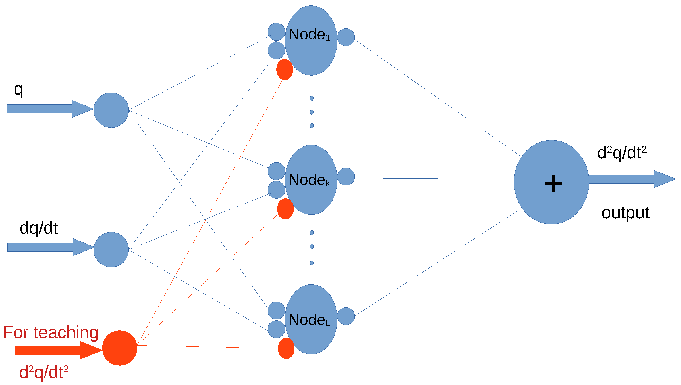
The above detailed abstract rotations were used as “activation functions” in the suggested new neural structure outlined in Figure 1 to describe the motion of the free van der Pol oscillator.
Similar to the feedforward neural networks, this new structure consists of an “input layer” that receives the input signals that in the case of the “learning phase” consists of the signals . The essential computation happens in the second layer that may contain many “nodes” receiving their input from the “input layer”, while the last, the third layer“ consist of a single element that simply summarizes the outputs obtained from the second layer. Like in the case of the polytopic models, a finite grid can be created for the input variable pairs . Each grid element can be characterized by its “range of competence” described by the disjoint intervals and . The neurons learn according to the following algorithm:
- Each neuron investigates if the input belongs to its range of competence. If then the given neuron (number i) is competent to make operation. In this case, in the learning phase, it
- associates the appropriate input value with the given grid element;
- augments the vector into , into in which and are the “dummy components” that guarantee the common norm ;
- calculates the unit vectors , and the angle of abstract rotation, , and finally
- if the place of the appropriate node is still empty, simply stores the computed data in the hyper-matrix as , , and where the subscripts and now denote the number of the given cell/node.
- If the node already is filled in, it either does nothing (simple skips the operation), or applies “incremental learning”.
“Incremental learning” means that instead of replacing the old node content with the new one, their weighted combination is calculated and will replace the old value. In the case of a scalar quantity x means that “the new value to be stored” () is calculated by the use of the previously stored “old value” () and the “new observed value” () with an “aggregation factor” as . This updating rule can be applied for the angle of the abstract rotation . The idea can be extended for the aggregation of unit vectors in the following approximate manner: the linear combination of not exactly parallel unit vectors must be a unit vector, i.e., the equations as follows must be valid:
in which
as
with two possible solutions as
of which the reasonable one is
Since as a scalar product of two unit vectors , , and since , the practical solution in (10) always can be chosen. For identical unit vectors and the same rule applied for the scalars, i.e., using the weighting factors and is obtained. Furthermore, if then for an arbitrary possible S, i.e., the old vector remains invariant (no aggregation is happening). Similarly, if then for an arbitrary possible S is yielded, i.e., simply the old vector will be replaced by the new one.
The above rule can be applied for the aggregation of the unit vectors and . Since it cannot be expected that the new aggregated unit vectors remain exactly orthogonal to each other, the matrix in (4) will not remain exactly an orthogonal one. However, since for not very different unit vectors , the new unit vectors and remain almost orthogonal to each other, consequently (4) can be considered to be a quickly calculable approximation of an orthogonal matrix.
Evidently this model in the “operation phase” can be used as follows:
- 1.
- For a given pair each neuron determines whether the input belongs to the box associated with its “competence of operation”: if not, the output value will be zero, otherwise it completes the following calculations:
- 2.
- the neuron retrieves the parameters of the activation function as , , and ,
- 3.
- computes the orthogonal matrix O in (4);
- 4.
- augments the vector into , where d is the physically not interpreted “dummy component”;
- 5.
- computes the rotated vector , and uses its first component as obtained from this special model, and
- 6.
- optionally it can refresh the cell content via “incremental learning”.
The aim of the “incremental learning method” consists of refining the model. Each neuron belongs to a “range” determined by the grid cells, while the input values may be concentrated in different parts of the cells. In this case, some refinement of the model can be achieved. In Section 3 the above method is exemplified when the system learns the model of the van der Pol oscillator in free motion.
3. Teaching Example: The Free Motion of the van der Pol Oscillator
The appropriate simulations were made in Julia Language Version 1.5.1 (2020-08-25) that is a kind of compilation of the most efficient simulation languages that legally can be used free of charge [77]. Its running speed is comparable with that of the codes made in language C or some Assembler language; however, it appears as a conveniently applicable high-level programming language such as, e.g., MATLAB. The here-presented results were obtained by the program “VDP_free_motion.jl”. (It is available at the link given in Section entitled “Supplementary Materials”.) This code is a simple text file edited by the use of Atom 1.57.0 x64 that allows the use of very special characters in the variable names. The initial state of the free motion was m, m·s, the discrete time resolution of the simple Euler integration was s. The resolution of the grid was determined as follows: the cell size for q was m and the interval m was covered by the model; for m·s was chosen for covering the interval m·s. In the teaching process the already filled in cell remained invariant, which theoretically corresponds to the aggregation weight , in (10).
4. Controlled Motion of the van der Pol Oscillator Using the Novel Neural Model
To critically reveal the possible consequences of the modeling imprecisions the CTC scheme was selected since in the possession of an exact dynamic model it can asymptotically drive any initial error to zero. However, when the model in use is only an approximate one, the trajectory tracking is degraded though the PID-type feedback terms can keep the errors at bay. Therefore, this paradigm can critically reveal the consequences of modeling errors. It is detailed in the following.
4.1. The Computed Torque Control and the Robust VS/SM Schemata
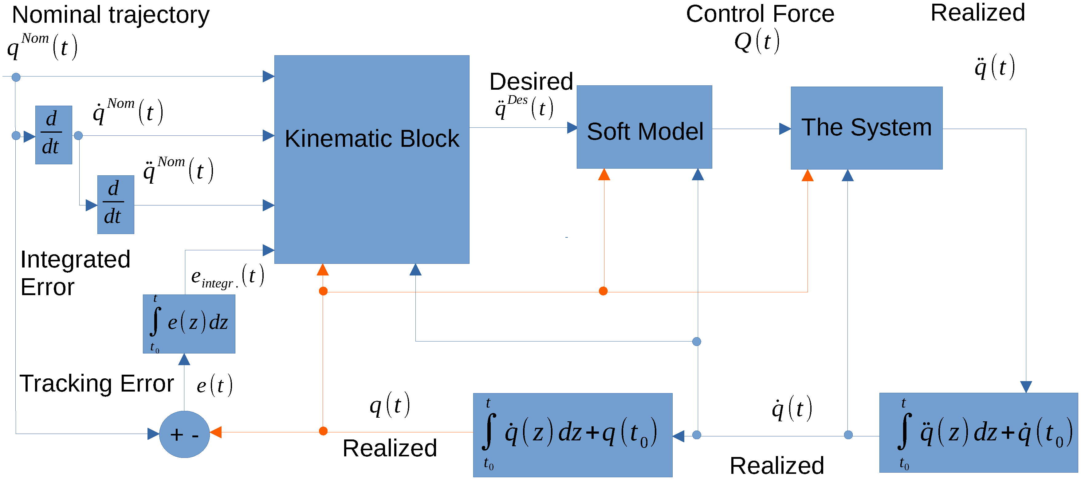
These control schemata are depicted in Figure 3, which easily can be followed when writing a simple sequential program code using Euler integration. The only difference between these schemata consists of the contents of the box “Kinematic Block”.
In the case of the CTC control the “Kinematic Block” in Figure 3 can be defined using an exponential parameter that is used for the calculation of the “desired” 2nd time-derivative in
Evidently (11) has the general solution of an LTI system that can be expressed by the linear combination of three basis functions as
in which the , and constants determine the initial conditions for the error quantities. Trivially, the operator maps to zero the function weighted by in (12). Similarly, the operator maps to zero the functions weighted by and , and finally, the operator maps to zero the functions weighted by , , and . Since each “basis function” converges to 0 as , the general solution also converges to zero if (11) is precisely realized. For this purpose, the exact system model is needed in Figure 3. If the system model is imprecise, no asymptotic convergence to zero can be expected.
In the case of the robust VS/SM controller, by maintaining the definition given in (11) for , , and , instead of (11), the desired 2nd time-derivative is computed as follows:
with the “damping”
leading to
Equation (14) has the following interpretation: for , i.e., the great S values with constant rate approach the value 0 that therefore approximately can be reached during finite time, and following that, S will be kept in the vicinity of 0 with the precision depending on the constant positive parameter w. This rate, and the precision by which S is subsequently kept near 0, also depends on the positive constant parameter K. According to (13) means that
of which it follows that after a few times time the quantity will become zero. In other words, will exponentially converge to 0. Evidently, (16) can be rearranged as follows:
that is a linear, time-invariant inhomogeneous differential equation in which the inhomogeneous driving term will vanish, and after that, the tracking error will exponentially converge to 0. The robustness of this construction simply consists of the fact that no precise realization of (14) is necessary. It is just enough to “somehow” make S quickly achieve 0, and following that, to “somehow” keep it near zero. For achieving this goal, no very precise system model is needed, and it can be expected that the deficiencies of the “soft model” can be compensated by choosing appropriate K and w parameters.
Since normally the control force Q with sharp jumps cannot be exactly tracked by real drives, and Figure 2 anticipates that small jumps can be expected when the firing neuron is changed, a signal smoothing technique that widely used in technical sciences for noise reduction (e.g., a second-order variant is used in [78]) was applied as follows. Let denote the rough signal obtained from the neural model that can contain jumps, and let denote its “smoothed” version applied in the control. Using a positive constant the smoothed signal must satisfy the differential equation
It is evident that for constant the stationary solution of (18) is . If is great enough can well track slowly varying signals while the abrupt jumps in are “filtered out” in this manner. In the following, the results of simulation investigations are presented for the CTC control.
4.2. Simulation Investigations
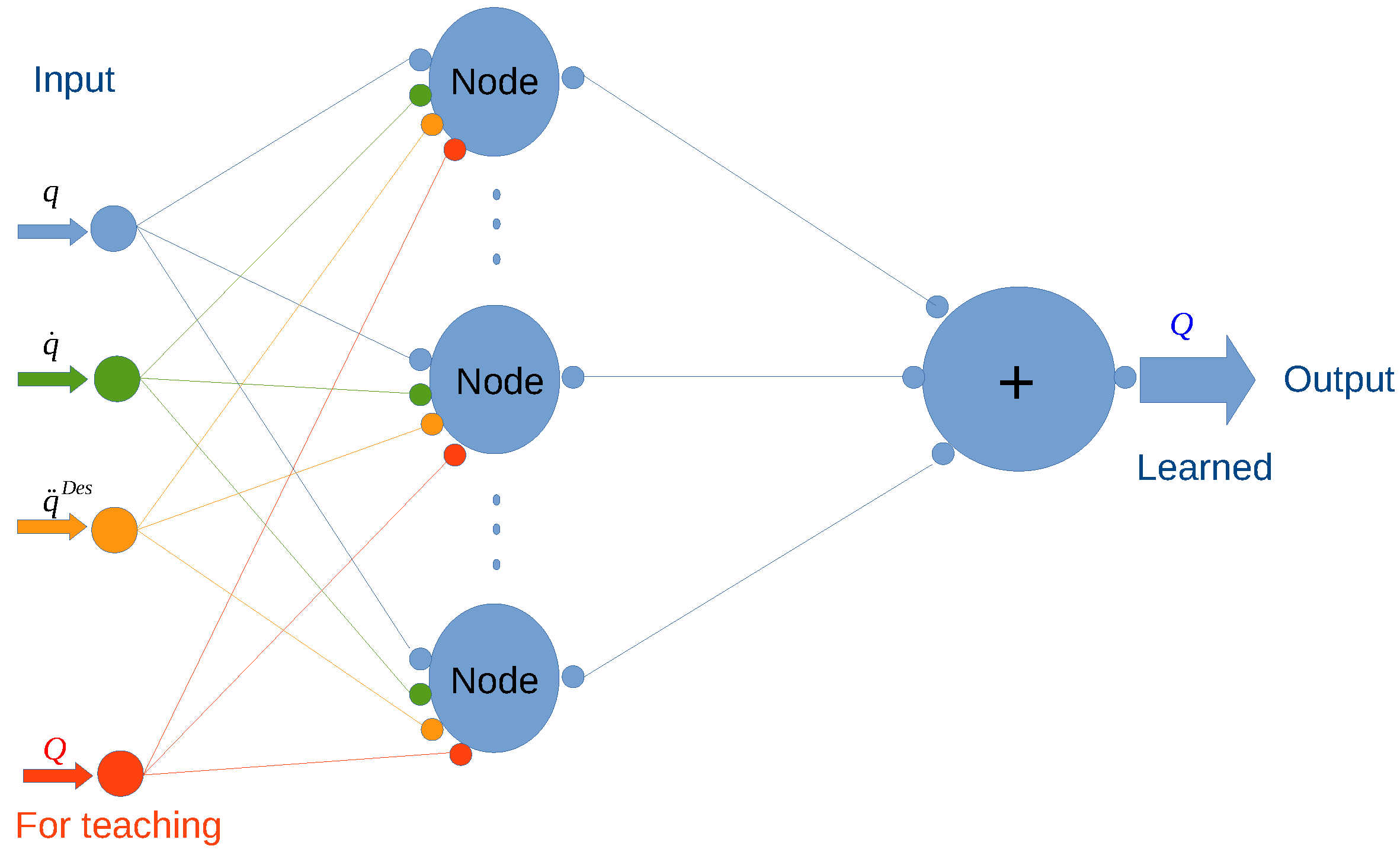
In this approach, the arrays were transformed into the vectors , therefore the augmented vectors had 4 components. The neuron structure is outlined in Figure 4.
Its teaching and operation is in strict analogy with that of the structure given in Figure 1, therefore these details will not be repeated here. For simulation purposes the Julia language program “VDP_machines_learning.jl” exemplified the CTC control, and the program “VDP_machines_learning_VSSM.jl” represented the VS/SM control. (The codes are available at the link given in Section entitled “Supplementary Materials”.) Both programs used the parameters s discrete time resolution in the Euler integration, s, s, the norm of the augmented vectors was , for the aggregation of the unit vectors was chosen. In the VS/SM controller the further parameters in (14) were m·s, and m·s.
The resolution of the grid was determined as follows: the cell size for q was m and the interval m was covered by the model; for m·s was chosen for covering the interval m·s; for m·s was chosen for covering the interval m·s. The teaching section consisted of filling in the values at the box centers with the data computed from the analytical model. Later, these values were slightly modified due to the aggregation that happened during the controlled motion.
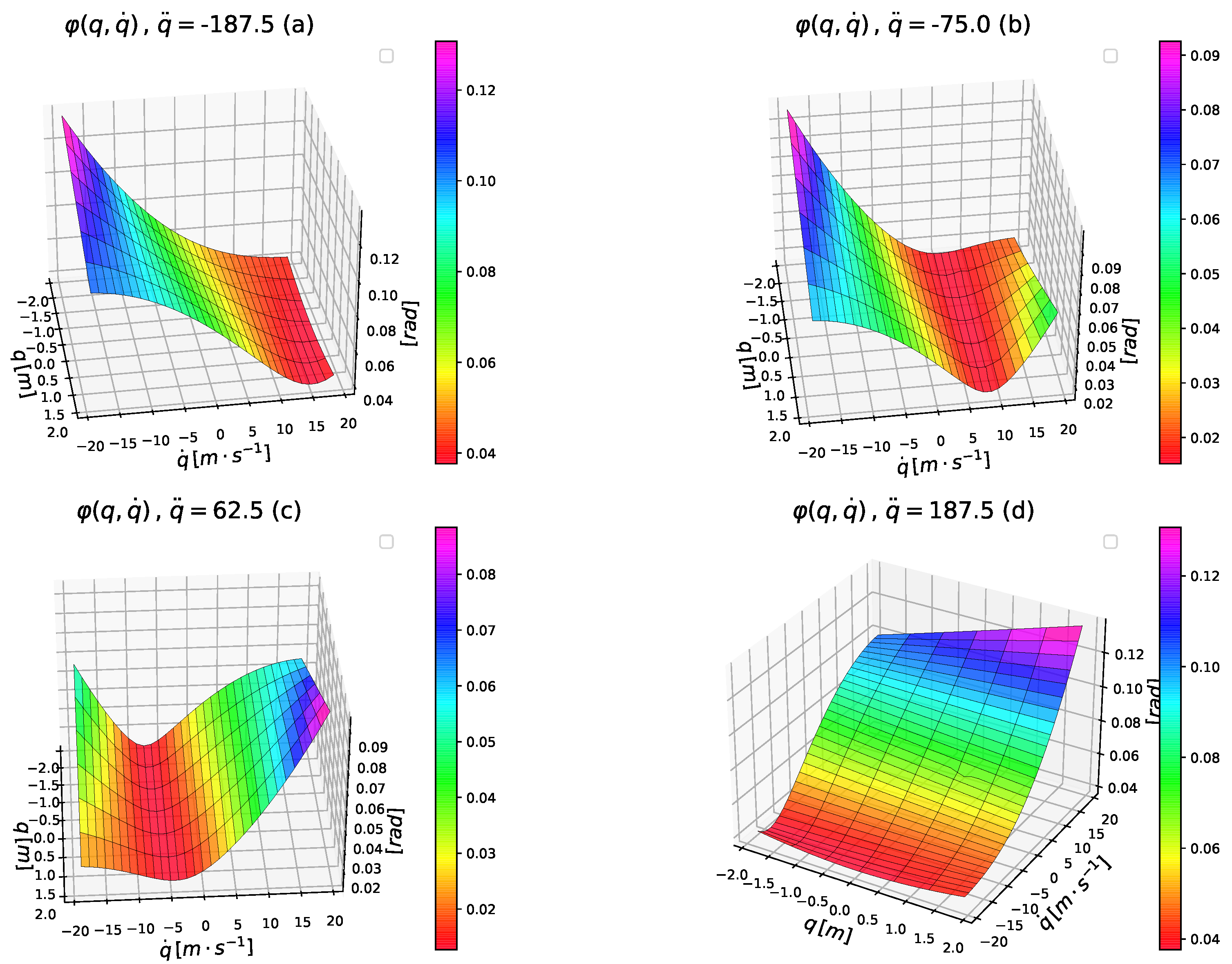
In the first set, the nominal trajectory was chosen to be a harmonic oscillation with the amplitude m and circular frequency s that is in the vicinity of the limit cycle of the oscillator’s motion (the data of which the grid limits were selected). Therefore, the best results were expected for this nominal trajectory. In Figure 5 the control surfaces expressed by the angle of the abstract rotations are described, just to illustrate certain internal details.
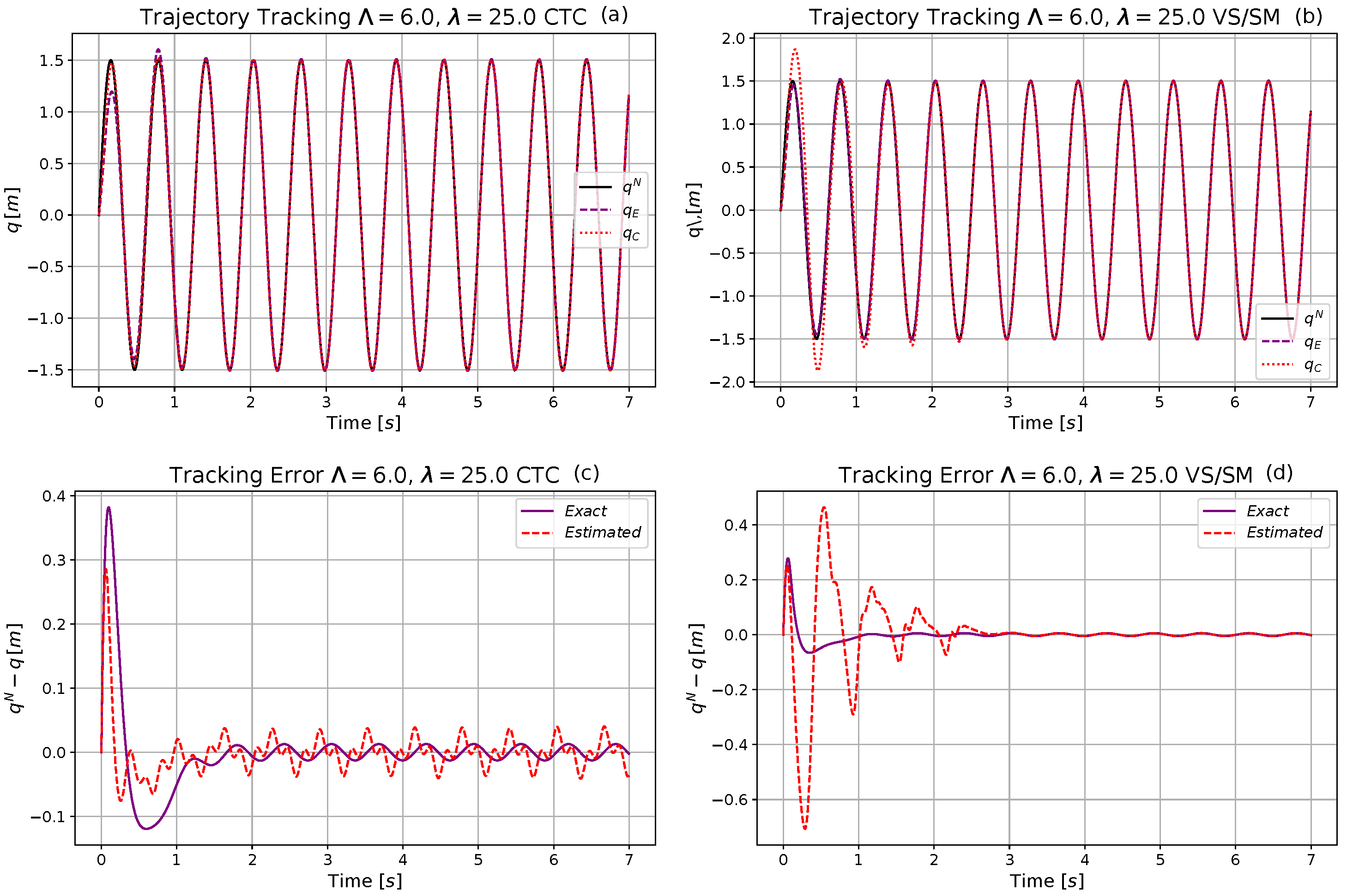
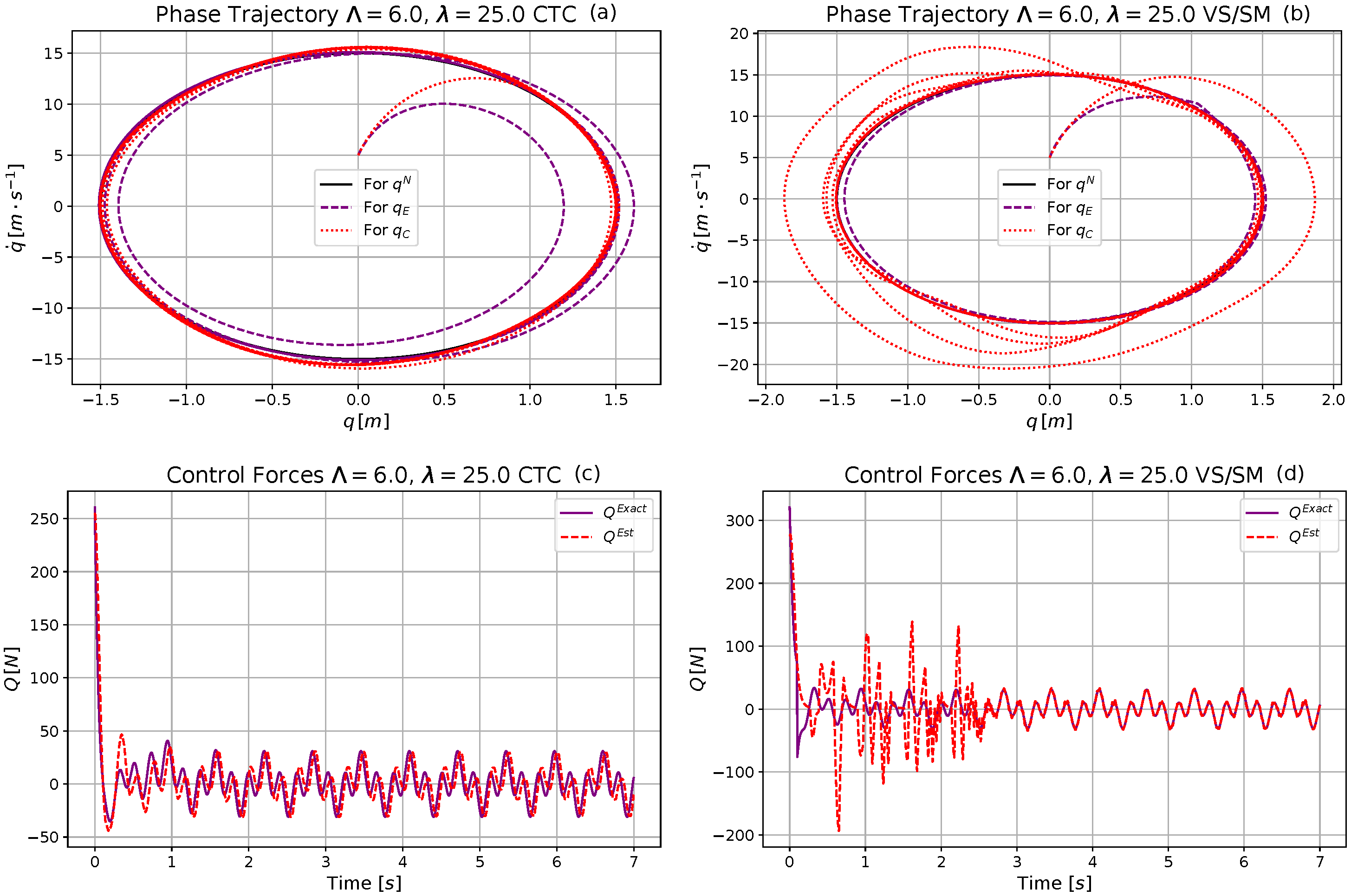
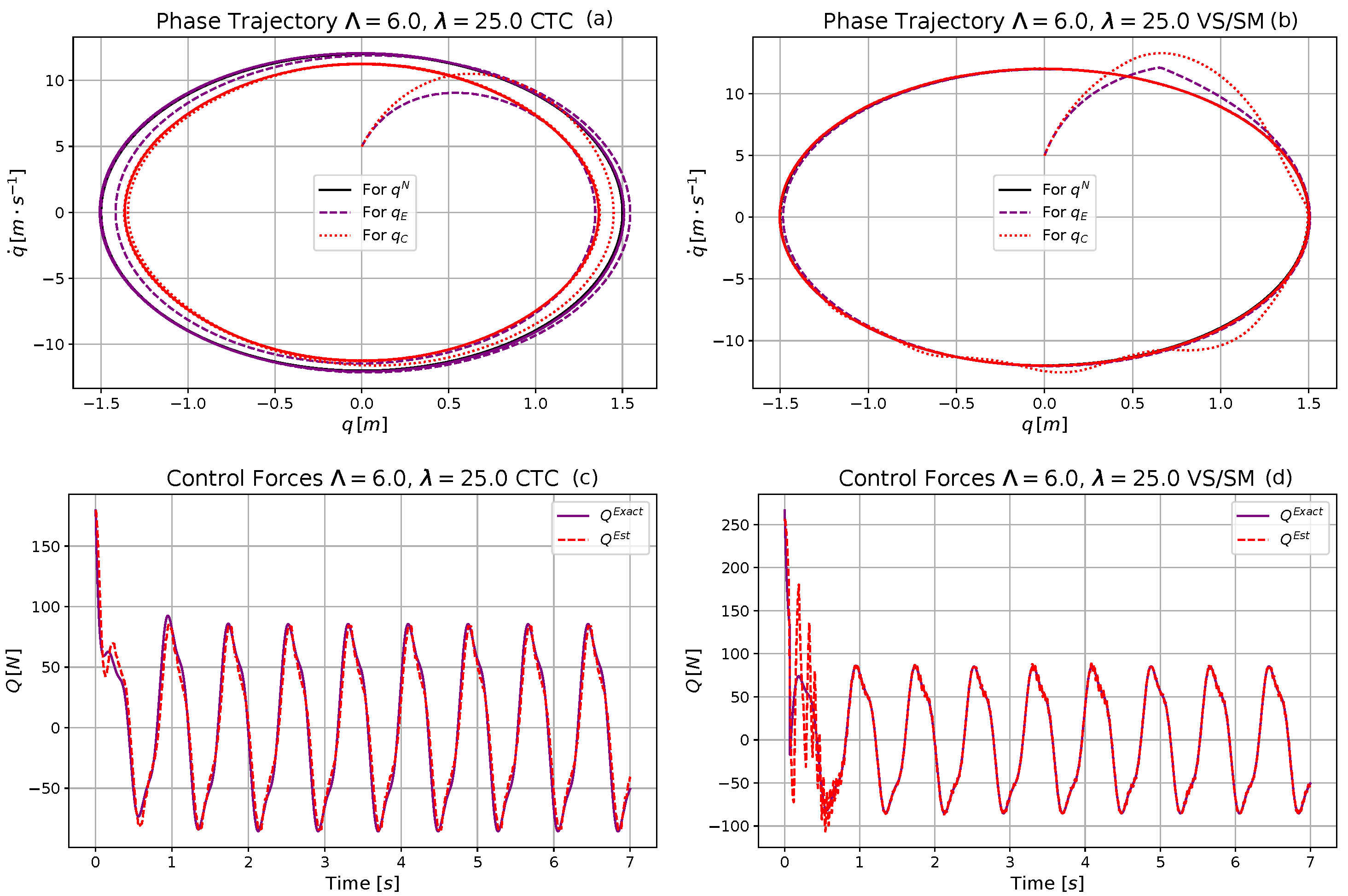
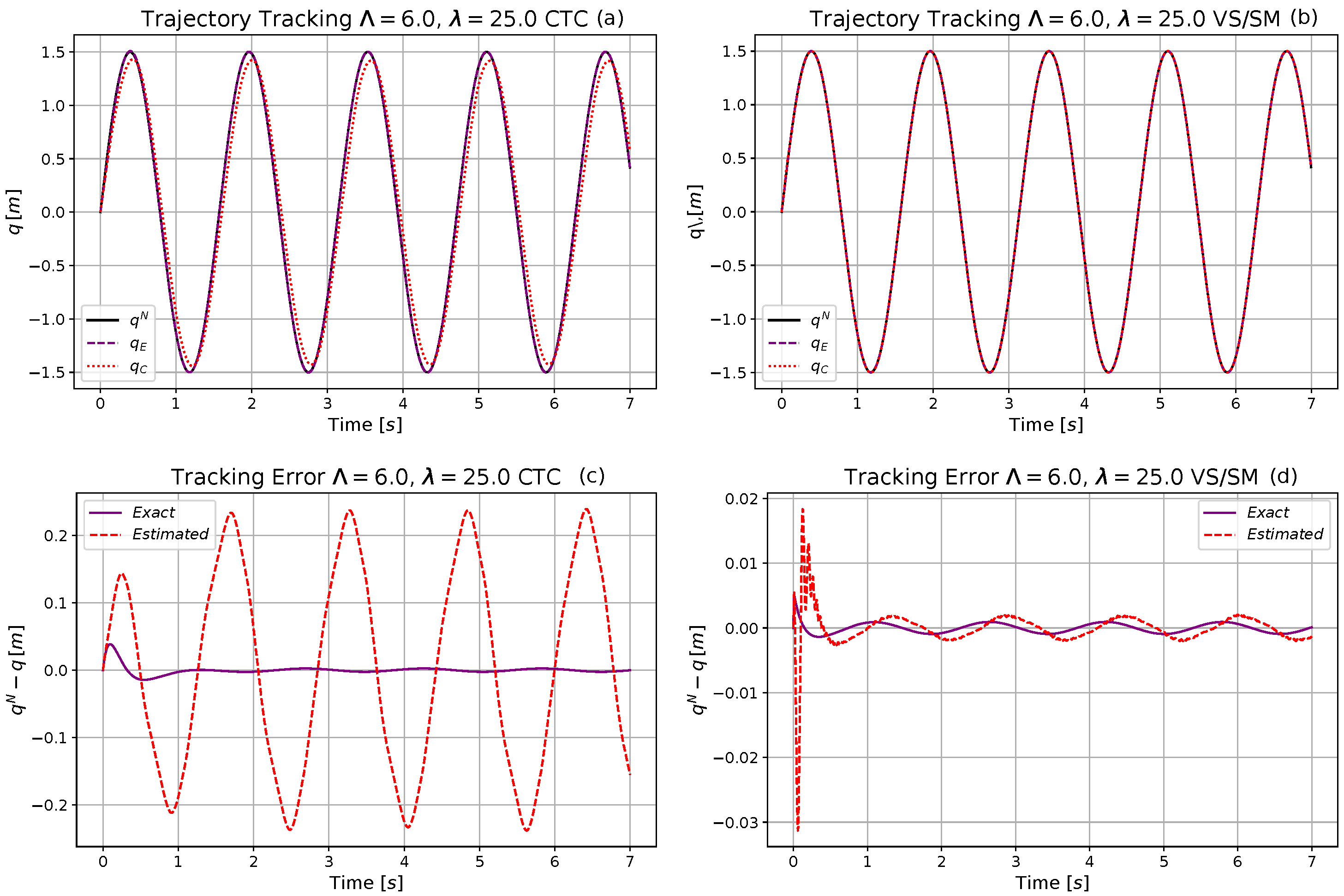
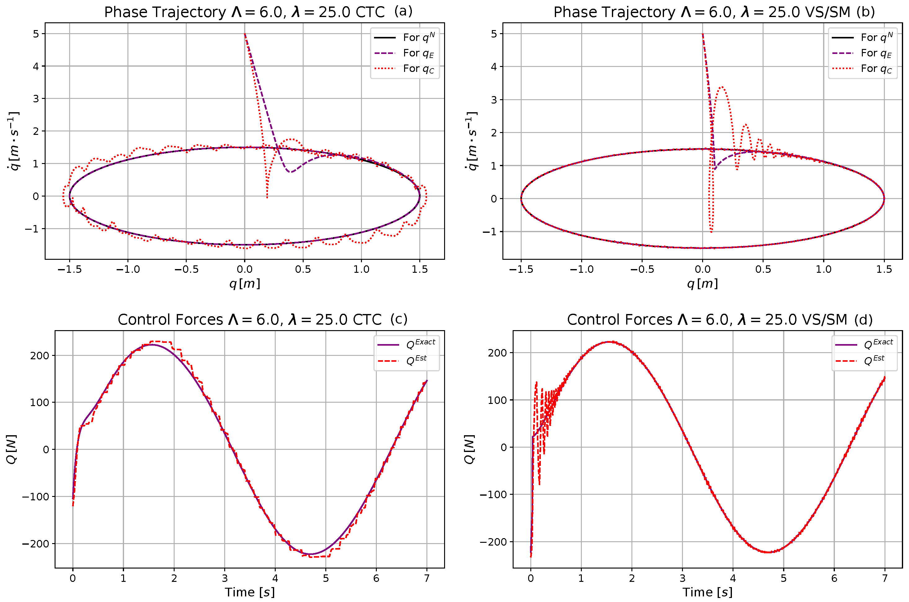
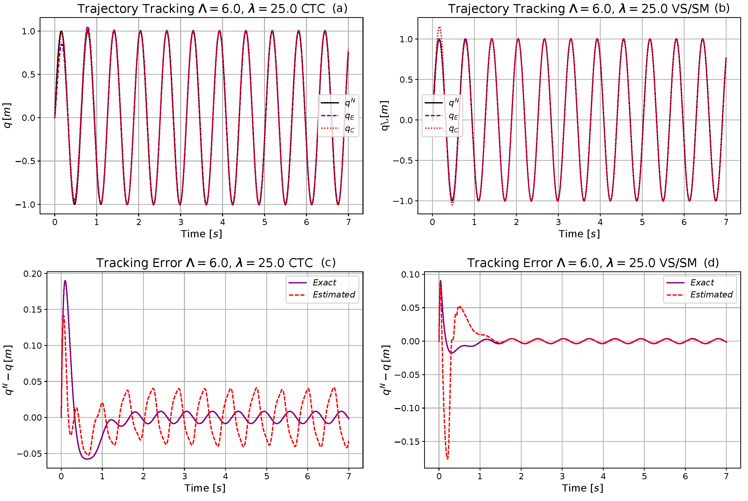
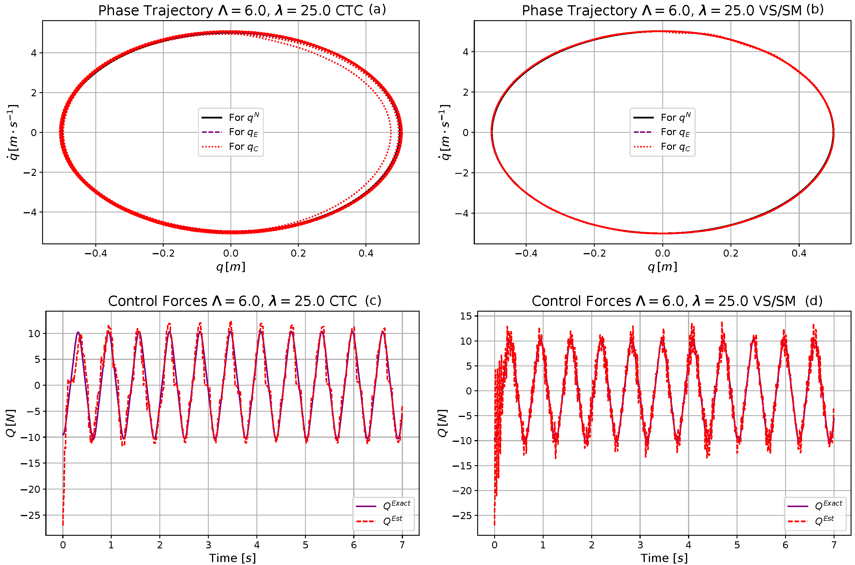
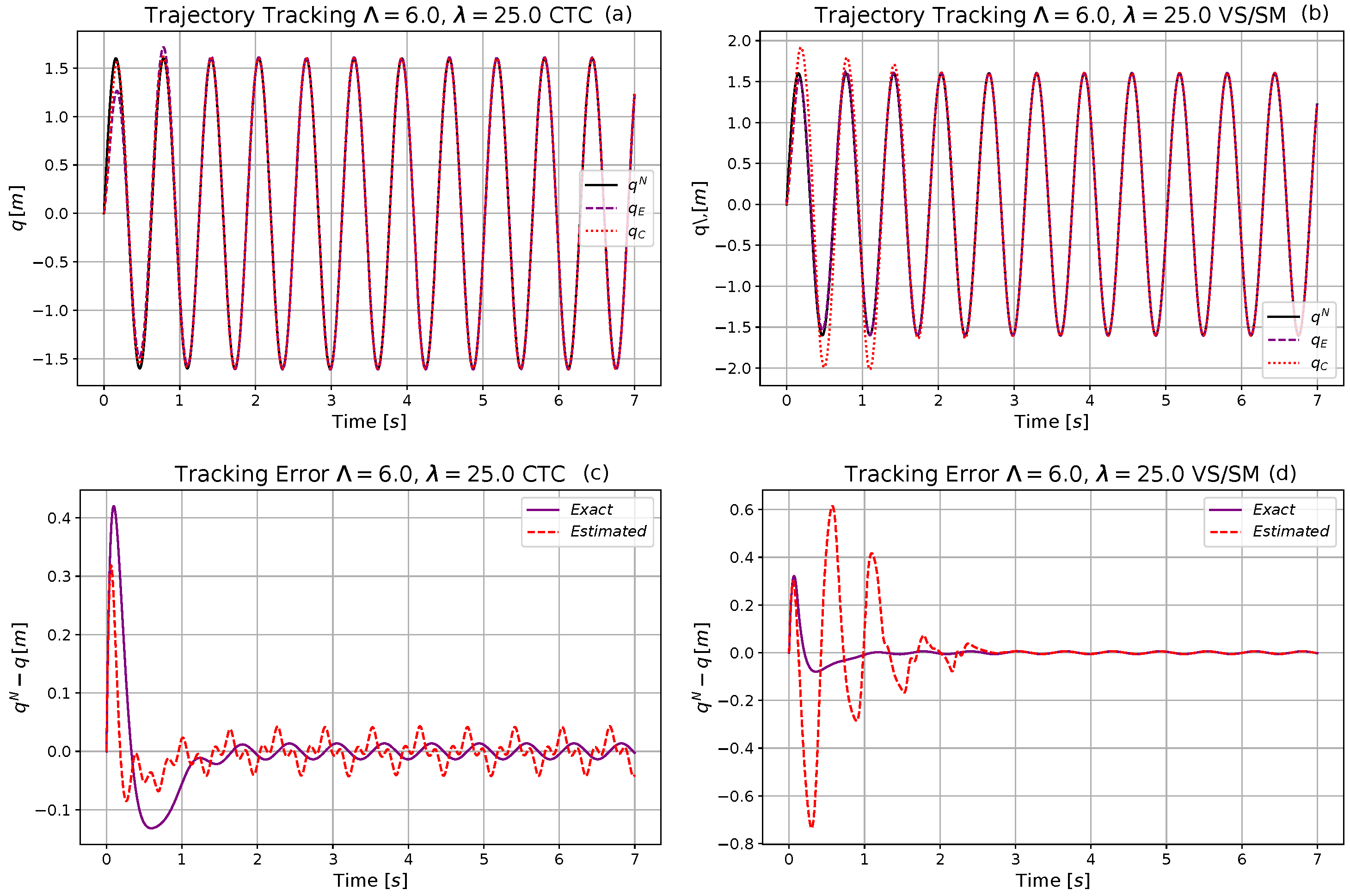
The trajectory tracking properties are given in Figure 6 and the phase trajectories and the control forces are described in Figure 7. It can be seen that the CTC controller works with small error, and using the kinematic prescription applied in the VS/SM control even this small error can be almost perfectly compensated. Following an initial transient phase, the trajectories and the forces applied by the VS/SM control practically become identical with the results using the exact dynamic model.
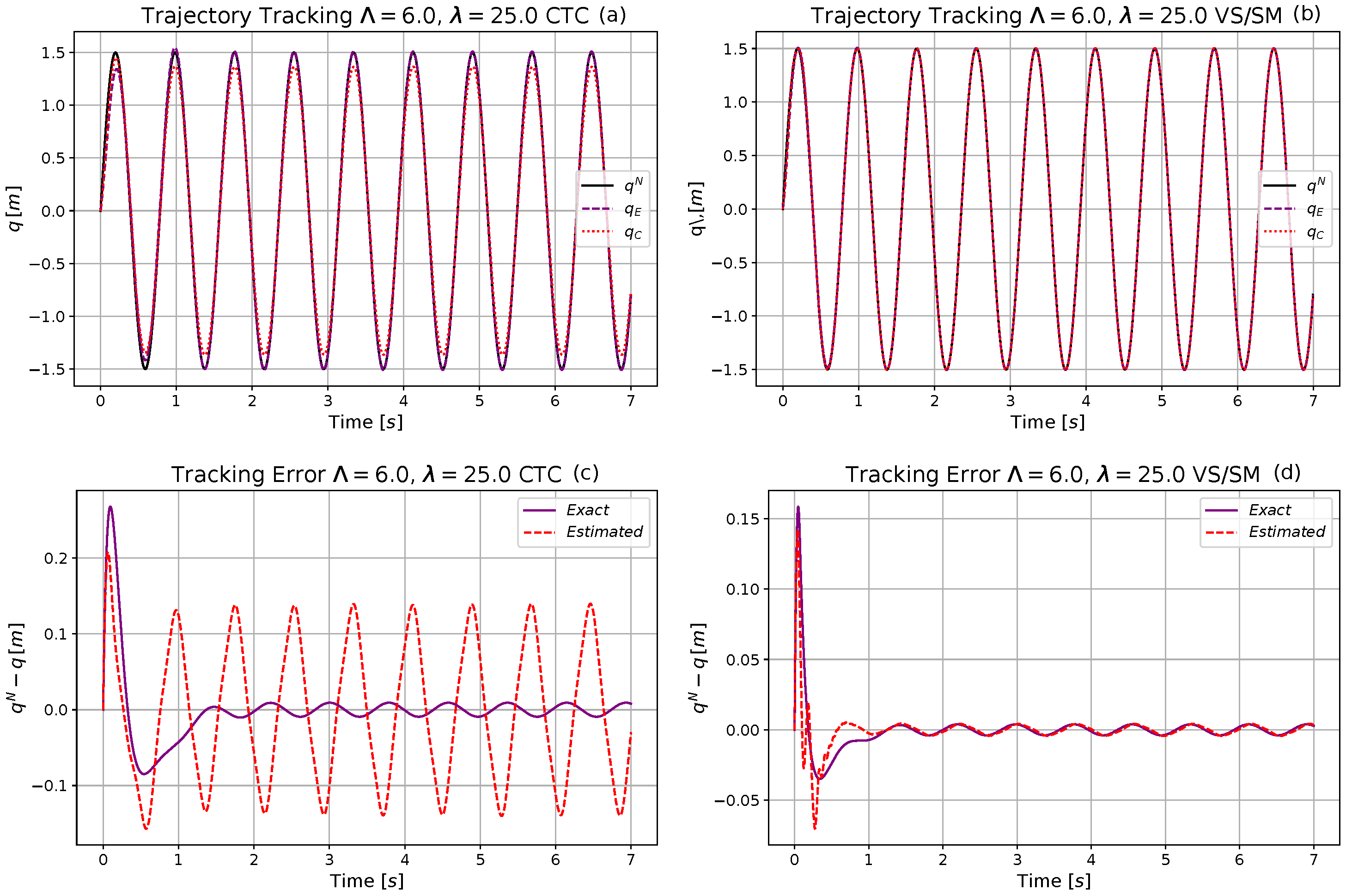
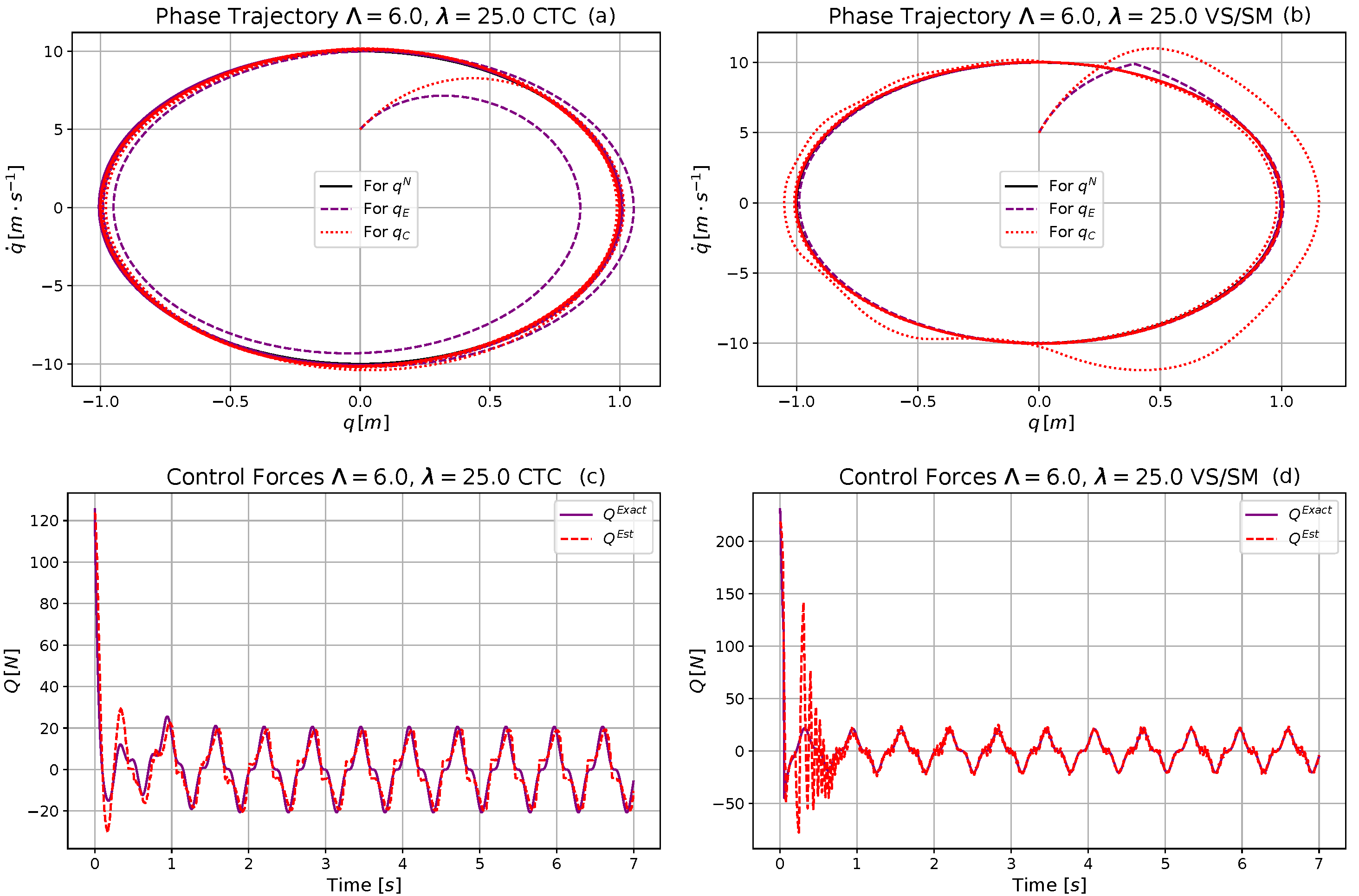
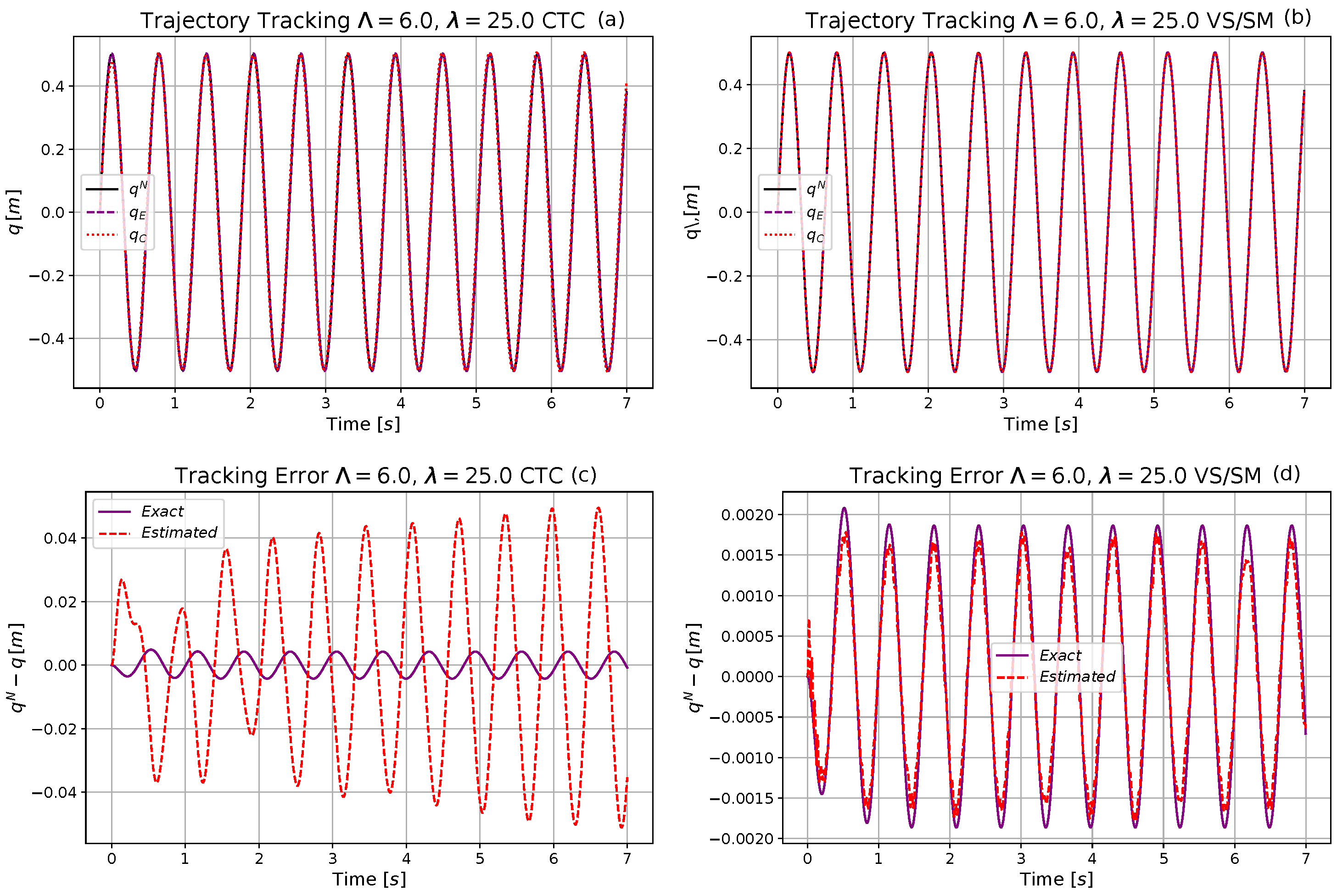
In the next step, the frequency of the nominal motion decreased to s while the amplitude remained invariant. In this case, the nominal motion to be tracked discovered other regions of the phase space. According to Figure 8 and Figure 9 it can be stated that the VS/SM controller again well corrected the small errors of the CTC controller.
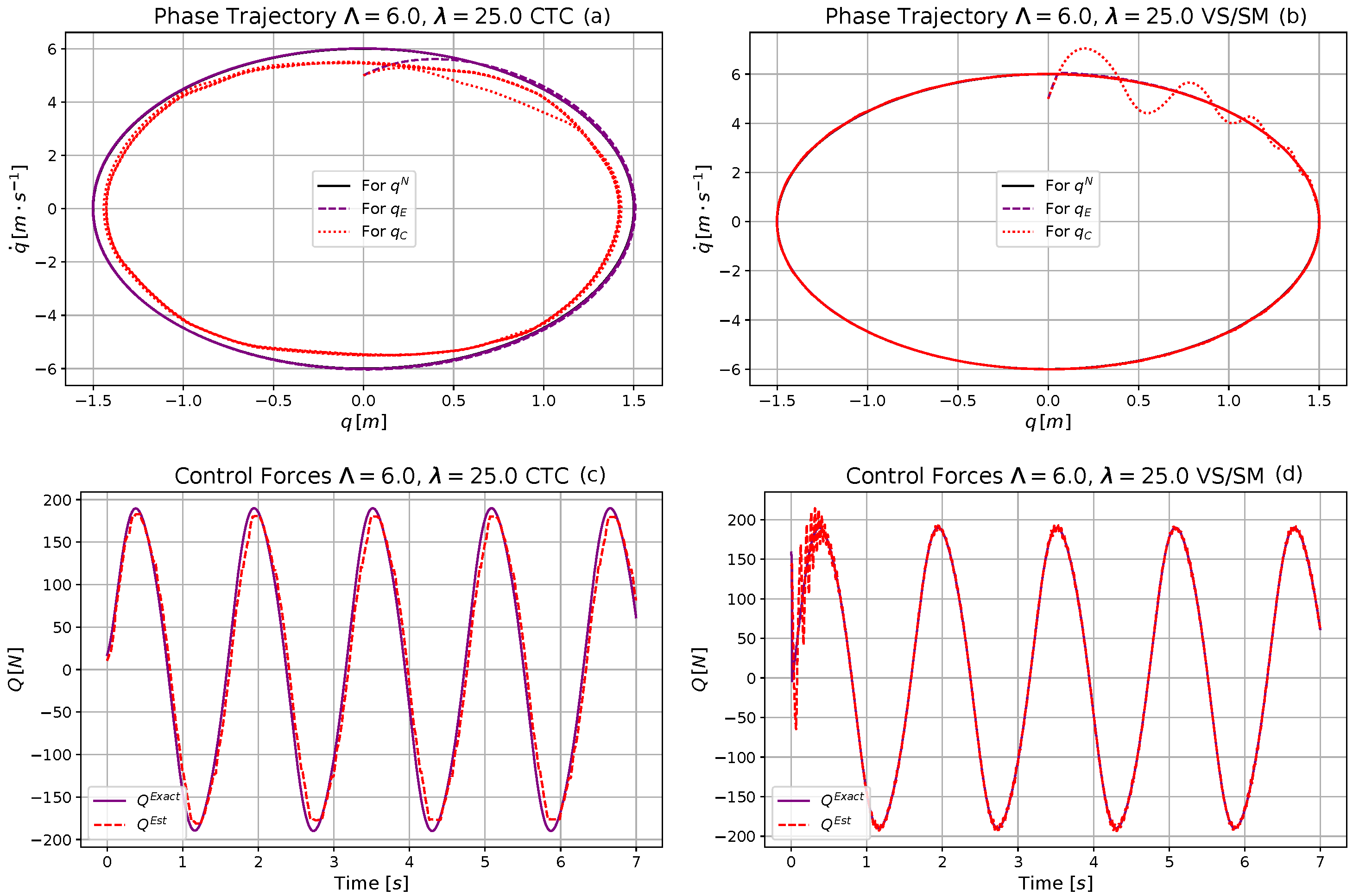
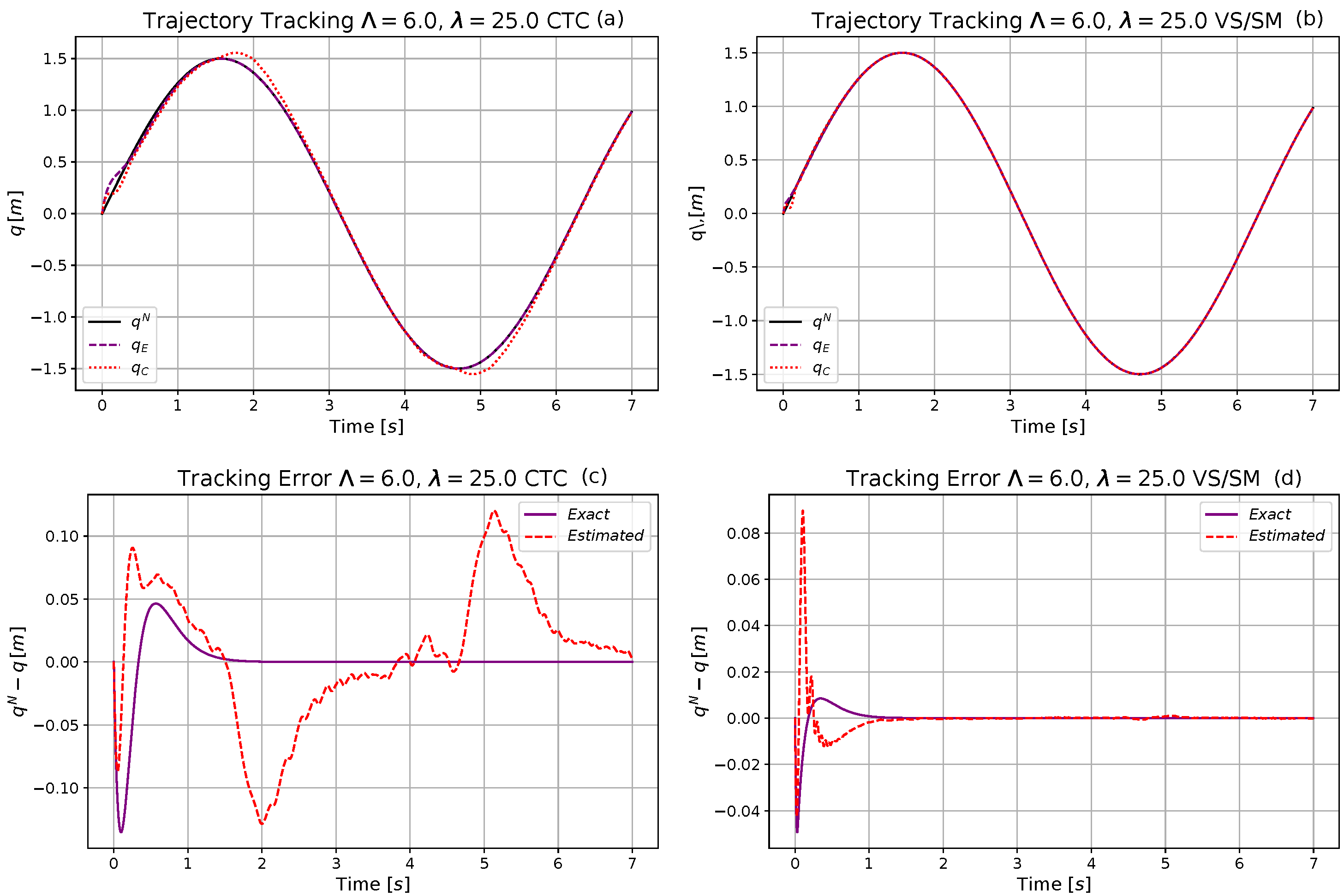
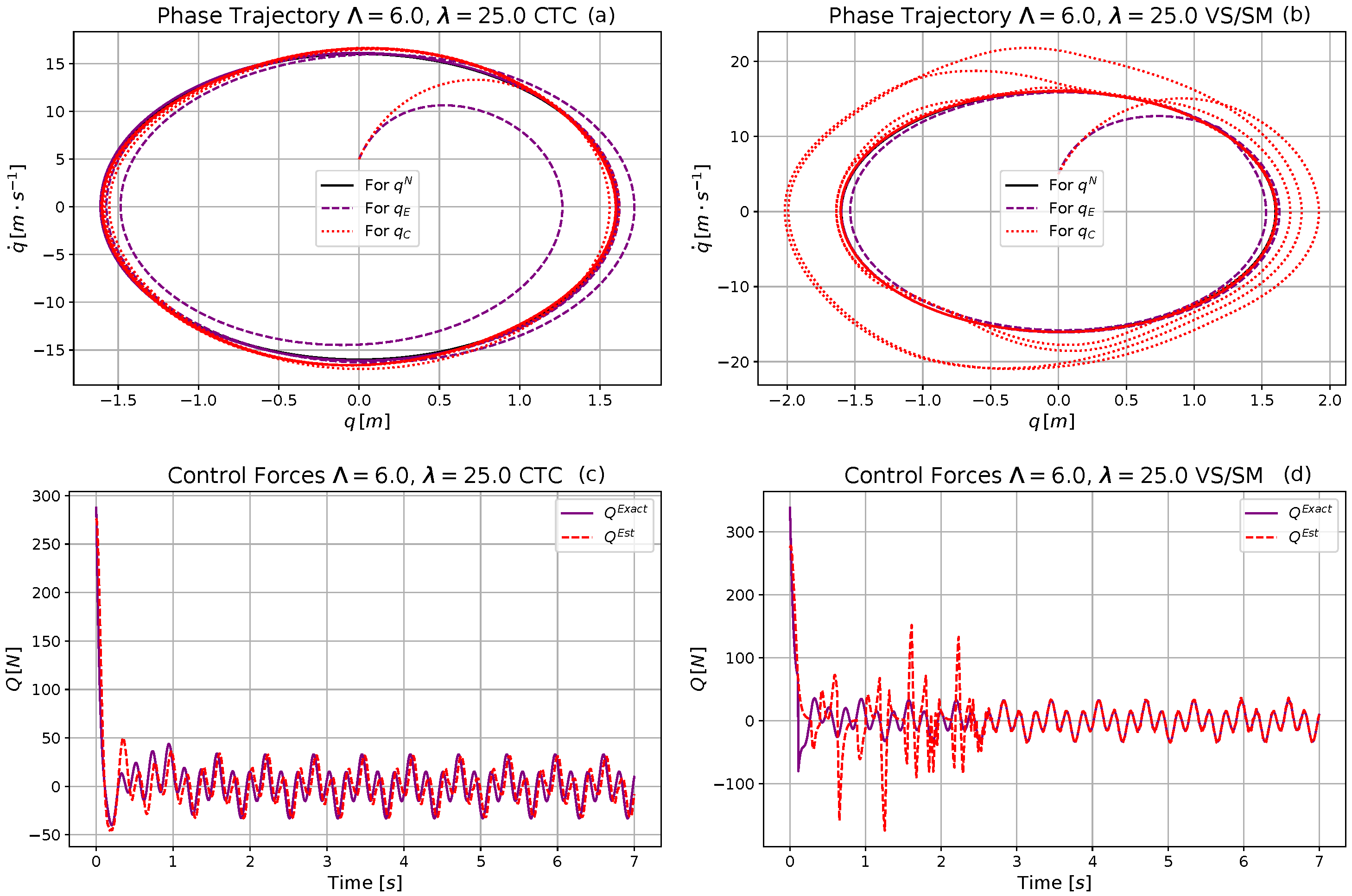
When the frequency of the nominal trajectory was further decreased to s in the phase trajectory, typical “deformations” appeared indicating that for this slow motion the resolution of the grid was found “rough”. However, the VS/SM control again well compensated the effects of the modeling errors (Figure 10 and Figure 11).
In the next series, the circular frequency of the nominal motion was reset to s but the amplitude was reduced to m to discover other regions of the map. Figure 14 and Figure 15 again reveal acceptable results.
For fast motion with small amplitude m and s can be selected, the results are given in Figure 16 and Figure 17 that show the same satisfactory effects.
The “generalizing” or “extrapolating” property of this structure can be checked by considering motions the appropriate data of which were not originally stored in the initial teaching process. Parameters m and s correspond to such a case. At this amplitude in the VS/SM control the m·s values frequently occur, for which the soft model does not contain appropriate cells. Consequently, it produces a longer fluctuating session before approaching the results of the controller that uses the “exact” model (Figure 18 and Figure 19). The CTC controller still works with small error. It can be stated that at this amplitude for s the “applicability limit” of this “soft model” has been found. (For the values m and s the VS/SM controller cannot capture the exact case and produces much worse results than the CTC controller.)
5. Conclusions
From a mathematical point of view, the soft computing-based modeling tools such as various neural networks, fuzzy system models and neurofuzzy systems are technical implementations of universal approximators that were elaborated for describing continuous functions. They generally can be used for describing various approximate dynamical system models for the precise construction of which no satisfactory physical basis is available. Such a “soft model” is coded in the form of algebraic combination of certain particular functions and the stored parameters of these functions. The practical use of the model means that depending on the model’s actual input, these functions must make real-time computation, and for obtaining the model’s output sophisticated data synchronization methods must be applied. Depending on the model structure teaching and using these models normally mean more or less massive parallelism based on distributed computing units. The whole family of these models suffers from the “curse of dimensionality” that practically means that for achieving “arbitrarily precise system models” huge structures must be used and tuned. Though since the pioneering work by Weierstraß in 1872 [79] (when he first constructed a nowhere differentiable continuous function) it can be known that the theoretical root of this problem is the “crazy nature” of the whole class of continuous functions, dimensionality is a serious issue even if smooth functions are assumed in the models. In the present paper, a novel neural network structure was suggested that has certain interesting and practical features as follows:
- Its activation function’s operation has simple geometric interpretation: it executes abstract rotations in higher-dimensional Euclidean spaces;
- The parameters of this function are encoded in two orthogonal unit vectors and in the angle of the abstract rotation that is executed by this function;
- The “extrapolation ability” of this function originates from the fact that with this rotation operator an array has to be transformed that conveys information on the “absolute value” of the modeled state;
- As with the polytopic models, the system model is so coded that each cell in a grid has its own activation function with its parameters;
- In contrast to the multilayer perceptrons or recurrent neural networks, no complicated “connecting wire structure” must be realized in its implementation;
- In contrast to the teaching phase of a multilayer perceptron, in which the error backpropagation requires the modification of the parameters of each function and the weight parameters in a massively parallel process, in this system only one neuron is active in a given time instant that is responsible for the necessary rotation. The other cells only must determine whether they must make any computation;
- In a similar manner, in the operating phase, when the model is in use, only one neuron executes the necessary transformation in a given time; the other ones only must check their competence. In contrast to that, the fuzzy inference systems must make massive distributed operations by executing the necessary “AND” and “OR” operations, fuzzification of the input and defuzzification of the output. Additionally, in the case of a multilayer perceptron, each neuron has to essentially take part in the computation of the final result that can be obtained by collecting the output of each neuron of a given layer, and forwarding their output to the neurons of the next layer;
- Due to the fact that the parameters of the functions are interpreted as orthogonal unit vectors, incremental adaptive improvement or “further teaching” of this model during its operation is possible by the use of a simple approximate “aggregation technique” that was elaborated for unit vectors.
In this paper, the above properties were exemplified in the case of a CTC controller that relatively is vulnerable to modeling errors. To compensate the effects of modeling imprecisions, the simple robust VS/SM was also applied in the control. The controlled system was the strongly nonlinear van der Pol oscillator that is a popular benchmark paradigm in control technology.
It is worth noting that, especially in control technology, modeling precision is not the “only”, and not necessarily the “most important” feature of a model. Possible small size, reduced complexity, and easy usability are important issues, too. Furthermore, robust as well as adaptive techniques can be applied for the compensation of the effects of various modeling imprecisions. In the present paper, a robust approach has been chosen for this purpose.
In future work, the noise-sensitivity of the method and time-delay problems must be investigated regarding this modeling method, in combination with the Fixed-Point Iteration-based adaptive approach that applies similar abstract rotations in Euclidean spaces to that of the “activation functions” of the suggested method.
Supplementary Materials
The following are available online at https://drive.google.com/drive/folders/1zuj9ncGtpbzBMWdq4HhR4o7KPJZ0mQo8?usp=sharing: “VDP_free_motion.jl”: Julia language code for exemplifying the learning process for free motion; “VDP_machines_learning.jl”: Julia language code exemplifying the controlled motion using CTC controller; “VDP_machines_learning_ VSSM.jl”: Julia language code exemplifying the controlled motion using VS/SM controller.
Author Contributions
Conceptualization, H.R.; Formal analysis, J.K.T.; Methodology, H.R.; Software, H.R.; Validation, J.K.T.; Writing—original draft, J.K.T. Both authors have read and agreed to the published version of the manuscript.
Funding
This research received no external funding.
Institutional Review Board Statement
Not applicable.
Informed Consent Statement
Not applicable.
Conflicts of Interest
The authors declare no conflict of interest.
References
- Yan, H. Reconstruction Designs of Lost Ancient Chinese Machinery; Springer: Dordrecht, The Netherlands, 2007. [Google Scholar]
- Rossi, C.; Russo, F. Automata (Towards Automation and Robots), Ancient Engineers’ Inventions; Springer: Dordrecht, The Netherlands, 2017; pp. 353–380. [Google Scholar]
- Hills, R. Power from the Wind; Cambridge University Press: Cambridge, UK, 1996. [Google Scholar]
- Maxwell, J. On Governors. Proc. R. Soc. 1868, 16, 270–283. [Google Scholar]
- Lyapunov, A. A General Task about the Stability of Motion. Ph.D. Thesis, University of Kazan, Tatarstan, Russia, 1892. (In Russian). [Google Scholar]
- Lyapunov, A. Stability of Motion; Academic Press: New York, NY, USA; London, UK, 1966. [Google Scholar]
- Lagrange, J.; Binet, J.; Garnier, J. Mécanique Analytique (Analytical Mechanics); Binet, J.P.M., Garnier, J.G., Eds.; Ve Courcier: Paris, France, 1811. [Google Scholar]
- Canudas de Wit, C.; Olsson, H.; Åström, K.; Linschinsky, P. Dynamic friction models and control design. In Proceedings of the 1993 American Control Conference, San Francisco, CA, USA, 2–4 June 1993; Volume 40, pp. 1920–1926. [Google Scholar]
- Márton, L.; Lantos, B. Identification and Model-based Compensation of Striebeck Friction. Acta Polytech. Hung. 2006, 3, 45–58. [Google Scholar]
- Armstrong, B.; Khatib, O.; Burdick, J. The Explicit Dynamic Model and Internal Parameters of the PUMA 560 Arm. In Proceedings of the 1986 IEEE International Conference on Robotics and Automation, San Francisco, CA, USA, 7–10 April 1986; pp. 510–518. [Google Scholar]
- Corke, P.; Armstrong-Helouvry, B. A Search for Consensus Among Model Parameters Reported for the PUMA 560 Robot. In Proceedings of the 1994 IEEE International Conference on Robotics and Automation, San Diego, CA, USA, 8–13 May 1994; pp. 1608–1613. [Google Scholar]
- Bergman, R.; Ider, Y.; Bowden, C.; Cobelli, C. Quantitative estimation of insulin sensitivity. Am. J. Physiol. Endocrinol. Metab. 1979, 236, E667–E677. [Google Scholar] [CrossRef] [PubMed]
- Sörensen, J. A Physiologic Model of Glucose Metabolism in Man and Its use to Design and Assess Improved Insulin Therapies for Diabetes. Ph.D. Thesis, Massachusetts Institute of Technology, Cambridge, MA, USA, 1985. [Google Scholar]
- Man, C.D.; Rizza, R.; Cobelli, C. Meal simulation model of glucose-insulin system. IEEE Trans. Biomed. Eng. 2007, 54, 1740–1749. [Google Scholar] [PubMed]
- Man, C.D.; Micheletto, F.; Lv, D.; Breton, M.; Kovatchev, B.; Cobelli, C. The UVA/PADOVA Type 1 Diabetes Simulator: New Features. J. Diabetes Sci. Technol. 2014, 8, 26–34. [Google Scholar] [CrossRef] [PubMed] [Green Version]
- Eigner, G.; Tar, J.; Rudas, I.; Kovács, L. LPV-based quality interpretations on modeling and control of diabetes. Acta Polytech. Hung. 2016, 13, 171–190. [Google Scholar]
- Andoga, R.; Főző, L. Near Magnetic Field of a Small Turbojet Engine. Acta Phys. Pol. 2017, 131, 1117–1119. [Google Scholar] [CrossRef]
- Andoga, R.; Főző, L.; Schrötter, M.; Češkovič, M.; Szabo, S.; Bréda, R.; Schreiner, M. Intelligent Thermal Imaging-Based Diagnostics of Turbojet Engines. Appl. Sci. 2019, 9, 2253. [Google Scholar] [CrossRef] [Green Version]
- Andoga, R.; Főző, L.; Judičák, J.; Bréda, R.; Szabo, S.; Rozenberg, R.; Džunda, M. Intelligent Situational Control of Small Turbojet Engines. Int. J. Aerosp. Eng. 2018, 2018, 1–16. [Google Scholar] [CrossRef]
- Andoga, R.; Főző, L.; Kovács, R.; Beneda, K.; Moravec, T.; Schreiner, M. Robust Control of Small Turbojet Engines. Machines 2019, 7, 3. [Google Scholar] [CrossRef] [Green Version]
- Főző, L.; Andoga, R.; Kovács, L.; Schreiner, M.; Beneda, K.; Savka, J.; Soušek, R. Virtual Design of Advanced Control Algorithms for Small Turbojet Engines. Acta Polytech. Hung. 2019, 16, 101–117. [Google Scholar] [CrossRef]
- Emelyanov, S.; Korovin, S.; Levantovsky, L. Higher Order Sliding Regimes in the Binary Control Systems. Sov. Phys. 1986, 31, 291–293. [Google Scholar]
- Levant, A. Arbitrary-order Sliding Modes with Finite Time Convergence. In Proceedings of the the 6th IEEE Mediterranean Conference on Control and Systems, Alghero, Sardinia, Italy, 9–11 June 1998. [Google Scholar]
- Utkin, V. Sliding Modes in Optimization and Control Problems; Springer: New York, NY, USA, 1992. [Google Scholar]
- Tar, J.; Bitó, J.; Nádai, L.; Tenreiro Machado, J. Robust Fixed Point Transformations in Adaptive Control Using Local Basin of Attraction. Acta Polytech. Hung. 2009, 6, 21–37. [Google Scholar]
- Banach, S. Sur les opérations dans les ensembles abstraits et leur application aux équations intégrales (About the Operations in the Abstract Sets and Their Application to Integral Equations). Fund. Math. 1922, 3, 133–181. [Google Scholar] [CrossRef]
- Tar, J.; Rudas, I.; Dineva, A.; Várkonyi-Kóczy, A. Stabilization of a Modified Slotine-Li Adaptive Robot Controller by Robust Fixed Point Transformations. In Proceedings of the Recent Advances in Intelligent Control, Modelling and Simulation, Cambridge, MA, USA, 29–31 January 2014; pp. 35–40. [Google Scholar]
- Dineva, A.; Várkonyi-Kóczy, A.; Tar, J. Combination of RFPT-based Adaptive Control and Classical Model Identification. In Proceedings of the 2014 IEEE 12th International Symposium on Applied Machine Intelligence and Informatics (SAMI), Herl’any, Slovakia, 23–25 January 2014; pp. 35–40. [Google Scholar]
- Csanádi, B.; Galambos, P.; Tar, J.; Györök, G.; Serester, A. Revisiting Lyapunov’s Technique in the Fixed Point Transformation-based Adaptive Control. In Proceedings of the 2018 IEEE 22nd International Conference on Intelligent Engineering Systems (INES), Las Palmas de Gran Canaria, Spain, 21–23 June 2018; pp. 329–334. [Google Scholar] [CrossRef]
- Weierstraß, K. Über die analytische Darstellbarkeit sogenannter willkürlicher Functionen einer reellen Veränderlichen (About the analytical representability of so-called arbitrary functions of a real variable). Sitzungsberichte Akad. Berl. (Inaug. Lect. Acad. Berl.) 1885, 2, 789–805. [Google Scholar]
- Stone, M. A generalized Weierstrass approximation theorem. Math. Mag. 1948, 21, 237–254. [Google Scholar] [CrossRef]
- Wang, L.X.; Mendel, J. Fuzzy Basis Functions, Universal Approximation and Orthogonal Least Squares Learning. IEEE Trans. Neural Netw. 1992, 3, 807–814. [Google Scholar] [CrossRef] [Green Version]
- Hilbert, D. Mathematical Problems. Bull. Am. Math. Soc. 1902, 8, 437–479. [Google Scholar] [CrossRef] [Green Version]
- Kolmogorov, A. On the representation of continuous functions of many variables by superposition of continuous functions of one variable and addition (in Russian). Dokl. Akad. Nauk. SSSR 1957, 114, 953–956. [Google Scholar]
- Sprecher, D. On the Structure of Continuous Functions of Several Variables. Trans. Am. Math. Soc. 1965, 115, 340–355. [Google Scholar] [CrossRef]
- Lorentz, G. Approximation of Functions; Holt, Reinhard and Winston: New York, NY, USA, 1965. [Google Scholar]
- Volterra, V. Theory of Functionals and of Integrals and Integro-Differential Equations (Reprinted Translation of the Original Work in Spanish Issued in Madrid in 1927); Dover Publications: New York, NY, USA, 1959. [Google Scholar]
- Kůrková, V. Kolmogorov’s Theorem and Multilayer Neural Networks. Neural Netw. 1992, 5, 501–506. [Google Scholar] [CrossRef]
- Miyanawala, T.P.; Jaiman, R.K. An Efficient Deep Learning Technique for the Navier-Stokes Equations: Application to Unsteady Wake Flow Dynamics. arXiv 2018, arXiv:1710.09099v3. [Google Scholar]
- Hopfield, J. Neural networks and physical systems with emergent collective computational abilities. Proc. Natl. Acad. Sci. USA 1982, 79, 2554–2558. [Google Scholar] [CrossRef] [Green Version]
- Elman, J. Finding Structure in Time. Cogn. Sci. 1990, 14, 179–211. [Google Scholar] [CrossRef]
- Zadeh, L. Fuzzy Sets. Inf. Control 1965, 8, 338–353. [Google Scholar] [CrossRef] [Green Version]
- Kosko, B. Fuzzy Systems as Universal Approximators. In Proceedings of the IEEE International Conference on Fuzzy Systems, San Diego, CA, USA, 8–12 March 1992; pp. 1153–1162. [Google Scholar]
- Castro, J. Fuzzy Logic Controllers are Universal Approximators. IEEE Trans. SMC 1995, 25, 629–635. [Google Scholar] [CrossRef]
- Kohonen, T. Self-Organized Formation of Topologically Correct Feature Maps. Biol. Cybern. 1982, 43, 59–69. [Google Scholar] [CrossRef]
- Sekaj, I.; Veselý, V. Robust Output Feedback Controller Design: Genetic Algorithm Approach. IMA J. Math. Control Inf. 2005, 22, 257–265. [Google Scholar] [CrossRef]
- Kirkpatrick, S.; Gelatt, C.D.; Vecchi, M.P. Optimization by simulated annealing. Science 1983, 220, 671–680. [Google Scholar] [CrossRef] [PubMed]
- Kinnenbrock, W. Accelerating the Standard Backpropagation Method Using a Genetic Approach. Neurocomputing 1994, 6, 583–588. [Google Scholar] [CrossRef]
- Kennedy, J.; Eberhart, R. Particle swarm optimization. In Proceedings of the ICNN’95—International Conference on Neural Networks, Perth, Australia, 27 November–1 December 1995; Volume 4, pp. 1942–1948. [Google Scholar]
- Dantzig, G. Origins of the Simplex Method (TECHNICAL REPORT SOL 87-5); Systems Optimization Laboratory, Department of Operations Research, Stanford University: Stanford, CA, USA, 1987. [Google Scholar]
- Nelder, J.; Mead, R. A simplex method for function minimization. Comput. J. 1965, 7, 308–313. [Google Scholar] [CrossRef]
- Lagarias, J.; Reeds, J.; Wright, M.; Wright, P. Convergence properties of the Nelder-Mead simplex method in low dimensions. SIAM J. Optim. 1998, 9, 112–147. [Google Scholar] [CrossRef] [Green Version]
- Galántai, A. A convergence analysis of the Nelder-Mead simplex method. Acta Polytech. Hung. 2021, 18, 93–105. [Google Scholar] [CrossRef]
- Potter, M.; Jong, K. A cooperative coevolutionary approach to function optimization. In Proceedings of the International Conference on Evolutionary Computati on the Third Conference on Parallel Problem Solving from Nature—PPSN III, Jerusalem, Israel, 9–14 October 1994. [Google Scholar]
- Nishida, K.; Yamauchi, K. Detecting concept drift using statistical testing. In Proceedings of the 10th International Conference, (DS’07), Sendai, Japan, 1–4 October 2007; Volume 4755, pp. 264–269. [Google Scholar]
- Barros, R.; Santos, S. A large-scale comparison of concept drift detectors. Inf. Sci. 2018, 451–452, 348–370. [Google Scholar] [CrossRef]
- Baranyi, P.; Szeidl, L.; Várlaki, P.; Yam, Y. Definition of the HOSVD-based canonical form of polytopic dynamic models. In Proceedings of the 3rd International Conference on Mechatronics (ICM 2006), Budapest, Hungary, 3–5 July 2006; pp. 660–665. [Google Scholar]
- Baranyi, P.; Szeidl, L.; Várlaki, P.; Yam, Y. Numerical reconstruction of the HOSVD-based canonical form of polytopic dynamic models. In Proceedings of the 10th International Conference on Intelligent Engineering Systems, London, UK, 26–28 June 2006; pp. 196–201. [Google Scholar]
- Golub, G.; Kahan, W. Calculating the singular values and pseudoinverse of a matrix. SIAM J. Numer. Anal. 1965, 2, 205–224. [Google Scholar]
- Lathauwer, L.; Moor, B.; Vandewalle, J. A multilinear singular value decomposition. SIAM J. Matrix Anal. Appl. 2000, 21, 1253–1278. [Google Scholar] [CrossRef] [Green Version]
- Colaneri, P. Analysis and Control of Linear Switched Systems (Lecture Notes); Politecnico di Milano: Milan, Italy, 2009. [Google Scholar]
- Horváth, Z.; Edelmayer, A. Robust Model-Based Detection of Faults in the Air Path of Diesel Engines. Acta Univ. Sapientiae Electr. Mech. Eng. 2015, 7, 5–22. [Google Scholar]
- Eigner, G. Novel LPV-based Control Approach for Nonlinear Physiological Systems. Acta Polytech. Hung. 2017, 14, 45–61. [Google Scholar]
- Siciliano, B.; Khatib, O. Springer Handbook of Robotics; Springer: Cham, Switzerland, 2016. [Google Scholar]
- Lapicque, L. Recherches quantitatives sur l’excitation électrique des nerfs traitée comme une polarisation (Quantitative Research on the Electric Excitation of Nerves by Polarisation). J. Physiol. Pathol. 1907, 9, 620–635. [Google Scholar]
- Hodgkin, A.; Huxley, A. A quantitative description of membrane current and its application to conduction and excitation in nerve. J. Physiol. 1952, 117, 500–544. [Google Scholar] [CrossRef]
- Zhabotinsky, A. Periodic processes of malonic acid oxidation in a liquid phase. Biophysika 1964, 9, 306–311. [Google Scholar]
- Field, R.; Koros, E.; Noyes, R. Oscillations in Chemical Systems. II. Thorough Analysis of Temporal Oscillation in the Bromate-Cerium-Malonic Acid System. J. Am. Chem. Soc. 1972, 94, 8649–8664. [Google Scholar] [CrossRef]
- Tyson, J. The Belousov-Zhabotinskii Reaction—Lecture Notes in Biomathematics 10; Springer: Berlin/Heidelberg, Germany, 1976. [Google Scholar]
- Kondepudi, D.; Prigogine, I. Modern Thermodynamics; John Wiley & Sons: Chichester, UK, 1998. [Google Scholar]
- Matsumoto, T. A Chaotic Attractor from Chua’s Circuit. IEEE Trans. Circuits Syst. 1984, CAS-31, 1055–1058. [Google Scholar] [CrossRef]
- Lorenz, E. Deterministic nonperiodic flow. J. Atmos. Sci. 1963, 20, 130–141. [Google Scholar] [CrossRef] [Green Version]
- Mickens, R. Mathematical and numerical study of the Duffing-harmonic oscillator. J. Sound Vib. 2001, 244, 563–567. [Google Scholar] [CrossRef]
- van der Pol, B. Forced oscillations in a circuit with non-linear resistance (reception with reactive triode). Lond. Edinb. Dublin Philos. Mag. J. Sci. 1927, 7, 65–80. [Google Scholar] [CrossRef]
- Csanádi, B.; Galambos, P.; Tar, J.; Györök, G.; Serester, A. A Novel, Abstract Rotation-based Fixed Point Transformation in Adaptive Control. In Proceedings of the 2018 IEEE International Conference on Systems, Man, and Cybernetics (SMC2018), Miyazaki, Japan, 7–10 October 2018; pp. 2577–2582. [Google Scholar]
- Rodrigues, O. Des lois géometriques qui regissent les déplacements d’ un systéme solide dans l’ espace, et de la variation des coordonnées provenant de ces déplacement considérées indépendent des causes qui peuvent les produire (Geometric laws which govern the displacements of a solid system in space: And the variation of the coordinates coming from these displacements considered independently of the causes which can produce them). J. Math. Pures Appl. 1840, 5, 380–440. [Google Scholar]
- Bezanson, J.; Edelman, A.; Karpinski, S.; Shah, V. Julia. Available online: https://julialang.org (accessed on 5 May 2019).
- Lantos, B.; Bodó, Z. High Level Kinematic and Low Level Nonlinear Dynamic Control of Unmanned Ground Vehicles. Acta Polytech. Hung. 2019, 16, 97–117. [Google Scholar]
- Weierstraß, K. Über continuirliche Functionen eines reellen Arguments, die für keinen Werth des letzeren einen bestimmten Differentialquotienten besitzen, (On single variable continuous functions that nowhere are differentiable). In Königlich Preussichen Akademie der Wissenschaften, Mathematische Werke von Karl Weierstrass; Mayer & Mueller: Berlin, Germany, 1895; Volume 2, pp. 71–74. [Google Scholar]
Figure 1.
The structure of the nodes for an mapping used for checking the mapping abilities in the case of the function of the free motion of the van der Pol oscillator.
Figure 1.
The structure of the nodes for an mapping used for checking the mapping abilities in the case of the function of the free motion of the van der Pol oscillator.

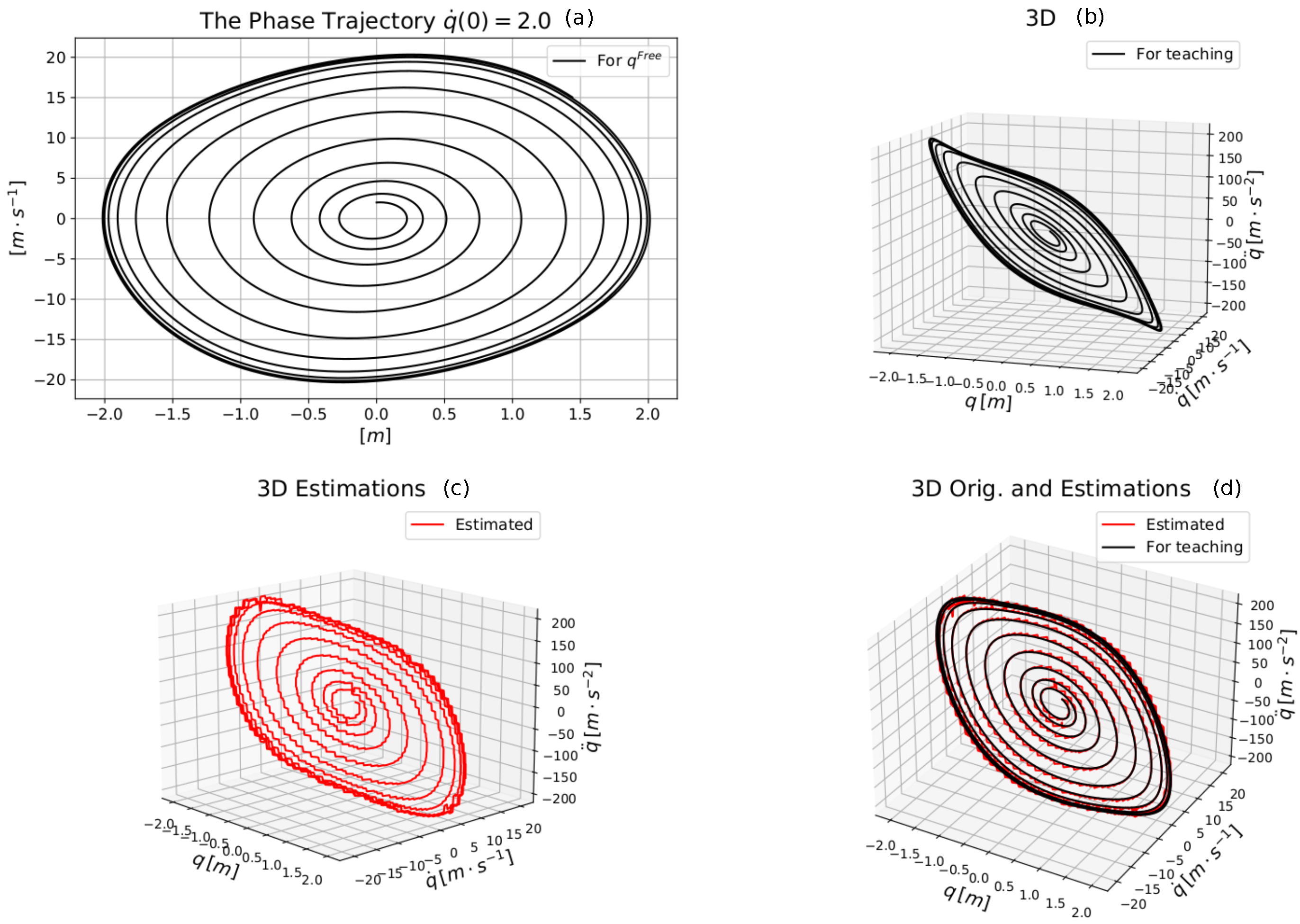
Figure 2.
Learning the free motion of the van der Pol oscillator: (a) The phase trajectory. (b) The values provided by the exact dynamic model. (c) The learned values retrieved from the neural model. (d) Comparison of the exact and the learned values.
Figure 2.
Learning the free motion of the van der Pol oscillator: (a) The phase trajectory. (b) The values provided by the exact dynamic model. (c) The learned values retrieved from the neural model. (d) Comparison of the exact and the learned values.

Figure 3.
The CTC and the robust VS/SM control schemata (the difference between these schemata consists of the contents of the box “Kinematic Block”).
Figure 3.
The CTC and the robust VS/SM control schemata (the difference between these schemata consists of the contents of the box “Kinematic Block”).

Figure 4.
The structure of the nodes for an mapping used for control purposes, i.e., for the approximation of the function .
Figure 4.
The structure of the nodes for an mapping used for control purposes, i.e., for the approximation of the function .

Figure 5.
Various projections of the stored control surfaces expressed by the angle of abstract rotations in the case of the CTC control.
Figure 5.
Various projections of the stored control surfaces expressed by the angle of abstract rotations in the case of the CTC control.

Figure 6.
Simulation results for trajectory tracking for amplitude m and circular frequency s: (a) Trajectory tracking of the CTC controller. (b) Trajectory tracking of the VS/SM controller. (c) Trajectory tracking error of the CTC controller. (d) Trajectory tracking error of the VS/SM controller.
Figure 6.
Simulation results for trajectory tracking for amplitude m and circular frequency s: (a) Trajectory tracking of the CTC controller. (b) Trajectory tracking of the VS/SM controller. (c) Trajectory tracking error of the CTC controller. (d) Trajectory tracking error of the VS/SM controller.

Figure 7.
Simulation results for amplitude m and circular frequency s: (a) Phase trajectory tracking of the CTC controller. (b) Phase trajectory tracking of the VS/SM controller. (c) Control force of the CTC controller. (d) Control force of the VS/SM controller.
Figure 7.
Simulation results for amplitude m and circular frequency s: (a) Phase trajectory tracking of the CTC controller. (b) Phase trajectory tracking of the VS/SM controller. (c) Control force of the CTC controller. (d) Control force of the VS/SM controller.

Figure 8.
Simulation results for trajectory tracking for amplitude m and circular frequency s: (a) Trajectory tracking of the CTC controller. (b) Trajectory tracking of the VS/SM controller. (c) Trajectory tracking error of the CTC controller. (d) Trajectory tracking error of the VS/SM controller.
Figure 8.
Simulation results for trajectory tracking for amplitude m and circular frequency s: (a) Trajectory tracking of the CTC controller. (b) Trajectory tracking of the VS/SM controller. (c) Trajectory tracking error of the CTC controller. (d) Trajectory tracking error of the VS/SM controller.

Figure 9.
Simulation results for amplitude m and circular frequency s: (a) Phase trajectory tracking of the CTC controller. (b) Phase trajectory tracking of the VS/SM controller. (c) Control force of the CTC controller. (d) Control force of the VS/SM controller.
Figure 9.
Simulation results for amplitude m and circular frequency s: (a) Phase trajectory tracking of the CTC controller. (b) Phase trajectory tracking of the VS/SM controller. (c) Control force of the CTC controller. (d) Control force of the VS/SM controller.

Figure 10.
Simulation results for trajectory tracking for amplitude m and circular frequency s: (a) Trajectory tracking of the CTC controller. (b) Trajectory tracking of the VS/SM controller. (c) Trajectory tracking error of the CTC controller. (d) Trajectory tracking error of the VS/SM controller.
Figure 10.
Simulation results for trajectory tracking for amplitude m and circular frequency s: (a) Trajectory tracking of the CTC controller. (b) Trajectory tracking of the VS/SM controller. (c) Trajectory tracking error of the CTC controller. (d) Trajectory tracking error of the VS/SM controller.

Figure 11.
Simulation results for amplitude m and circular frequency s: (a) Phase trajectory tracking of the CTC controller. (b) Phase trajectory tracking of the VS/SM controller. (c) Control force of the CTC controller. (d) Control force of the VS/SM controller.
Figure 11.
Simulation results for amplitude m and circular frequency s: (a) Phase trajectory tracking of the CTC controller. (b) Phase trajectory tracking of the VS/SM controller. (c) Control force of the CTC controller. (d) Control force of the VS/SM controller.

Figure 12.
Simulation results for trajectory tracking for amplitude m and circular frequency s: (a) Trajectory tracking of the CTC controller. (b) Trajectory tracking of the VS/SM controller. (c) Trajectory tracking error of the CTC controller. (d) Trajectory tracking error of the VS/SM controller.
Figure 12.
Simulation results for trajectory tracking for amplitude m and circular frequency s: (a) Trajectory tracking of the CTC controller. (b) Trajectory tracking of the VS/SM controller. (c) Trajectory tracking error of the CTC controller. (d) Trajectory tracking error of the VS/SM controller.

Figure 13.
Simulation results for amplitude m and circular frequency s: (a) Phase trajectory tracking of the CTC controller. (b) Phase trajectory tracking of the VS/SM controller. (c) Control force of the CTC controller. (d) Control force of the VS/SM controller.
Figure 13.
Simulation results for amplitude m and circular frequency s: (a) Phase trajectory tracking of the CTC controller. (b) Phase trajectory tracking of the VS/SM controller. (c) Control force of the CTC controller. (d) Control force of the VS/SM controller.

Figure 14.
Simulation results for trajectory tracking for amplitude m and circular frequency s: (a) Trajectory tracking of the CTC controller. (b) Trajectory tracking of the VS/SM controller. (c) Trajectory tracking error of the CTC controller. (d) Trajectory tracking error of the VS/SM controller.
Figure 14.
Simulation results for trajectory tracking for amplitude m and circular frequency s: (a) Trajectory tracking of the CTC controller. (b) Trajectory tracking of the VS/SM controller. (c) Trajectory tracking error of the CTC controller. (d) Trajectory tracking error of the VS/SM controller.

Figure 15.
Simulation results for amplitude m and circular frequency s: (a) Phase trajectory tracking of the CTC controller. (b) Phase trajectory tracking of the VS/SM controller. (c) Control force of the CTC controller. (d) Control force of the VS/SM controller.
Figure 15.
Simulation results for amplitude m and circular frequency s: (a) Phase trajectory tracking of the CTC controller. (b) Phase trajectory tracking of the VS/SM controller. (c) Control force of the CTC controller. (d) Control force of the VS/SM controller.

Figure 16.
Simulation results for trajectory tracking for amplitude m and circular frequency s: (a) Trajectory tracking of the CTC controller. (b) Trajectory tracking of the VS/SM controller. (c) Trajectory tracking error of the CTC controller. (d) Trajectory tracking error of the VS/SM controller.
Figure 16.
Simulation results for trajectory tracking for amplitude m and circular frequency s: (a) Trajectory tracking of the CTC controller. (b) Trajectory tracking of the VS/SM controller. (c) Trajectory tracking error of the CTC controller. (d) Trajectory tracking error of the VS/SM controller.

Figure 17.
Simulation results for amplitude m and circular frequency s: (a) Phase trajectory tracking of the CTC controller. (b) Phase trajectory tracking of the VS/SM controller. (c) Control force of the CTC controller. (d) Control force of the VS/SM controller.
Figure 17.
Simulation results for amplitude m and circular frequency s: (a) Phase trajectory tracking of the CTC controller. (b) Phase trajectory tracking of the VS/SM controller. (c) Control force of the CTC controller. (d) Control force of the VS/SM controller.

Figure 18.
Simulation results for trajectory tracking for amplitude m and circular frequency s: (a) Trajectory tracking of the CTC controller. (b) Trajectory tracking of the VS/SM controller. (c) Trajectory tracking error of the CTC controller. (d) Trajectory tracking error of the VS/SM controller.
Figure 18.
Simulation results for trajectory tracking for amplitude m and circular frequency s: (a) Trajectory tracking of the CTC controller. (b) Trajectory tracking of the VS/SM controller. (c) Trajectory tracking error of the CTC controller. (d) Trajectory tracking error of the VS/SM controller.

Figure 19.
Simulation results for amplitude m and circular frequency s: (a) Phase trajectory tracking of the CTC controller. (b) Phase trajectory tracking of the VS/SM controller. (c) Control force of the CTC controller. (d) Control force of the VS/SM controller.
Figure 19.
Simulation results for amplitude m and circular frequency s: (a) Phase trajectory tracking of the CTC controller. (b) Phase trajectory tracking of the VS/SM controller. (c) Control force of the CTC controller. (d) Control force of the VS/SM controller.

Publisher’s Note: MDPI stays neutral with regard to jurisdictional claims in published maps and institutional affiliations. |
© 2021 by the authors. Licensee MDPI, Basel, Switzerland. This article is an open access article distributed under the terms and conditions of the Creative Commons Attribution (CC BY) license (https://creativecommons.org/licenses/by/4.0/).
Share and Cite
MDPI and ACS Style
Redjimi, H.; Tar, J.K. A Simple Soft Computing Structure for Modeling and Control. Machines 2021, 9, 168. https://doi.org/10.3390/machines9080168
AMA Style
Redjimi H, Tar JK. A Simple Soft Computing Structure for Modeling and Control. Machines. 2021; 9(8):168. https://doi.org/10.3390/machines9080168
Chicago/Turabian StyleRedjimi, Hemza, and József Kázmér Tar. 2021. "A Simple Soft Computing Structure for Modeling and Control" Machines 9, no. 8: 168. https://doi.org/10.3390/machines9080168
Note that from the first issue of 2016, this journal uses article numbers instead of page numbers. See further details here.