
Adaptive Data-Driven Control for Linear Time Varying Systems


Department of Control and Computer Engineering, Politecnico di Torino, 10129 Turin, Italy
Machines 2021, 9(8), 167; https://doi.org/10.3390/machines9080167
Submission received: 14 July 2021
/
Revised: 7 August 2021
/
Accepted: 10 August 2021
/
Published: 13 August 2021
(This article belongs to the Special Issue Design and Control of Advanced Mechatronics Systems)
Abstract
:In this paper, we propose an adaptive data-driven control approach for linear time varying systems, affected by bounded measurement noise. The plant to be controlled is assumed to be unknown, and no information in regard to its time varying behaviour is exploited. First, using set-membership identification techniques, we formulate the controller design problem through a model-matching scheme, i.e., designing a controller such that the closed-loop behaviour matches that of a given reference model. The problem is then reformulated as to derive a controller that corresponds to the minimum variation bounding its parameters. Finally, a convex relaxation approach is proposed to solve the formulated controller design problem by means of linear programming. The effectiveness of the proposed scheme is demonstrated by means of two simulation examples.
1. Introduction
In the context of controlling linear time varying (LTV) systems, one of the most common approaches is adaptive control. This is due to the nature of these type of controllers, as they are capable of adjusting their parameters to cope of with the variations in the system to be controlled. Adaptive control techniques for LTV systems are not new and this problem has received great research efforts. A model reference adaptive control (MRAC) scheme is proposed in [1,2], while in [3,4], indirect adaptive schemes are considered for the case of slowly varying systems. In [5], an indirect adaptive pole placement is proposed for LTV systems with unmodeled dynamics and bounded disturbance. A linear periodic controller is presented in [6], where instead of estimating the plant and controller parameters, the ideal control signal is directly computed. In [7], an adaptive output feedback based controller is addressed, having a fixed structure that depends on the relative degree of the plant.
All of the aforementioned approaches rely on the presence of a model for the plant, or at least some sort of description for its dynamics and structure. In many control applications, deriving a mathematical representation for the plant to be controlled may not be an easy task, as the dynamics of the system may be too complex and may require extensive efforts in order to find a suitable model. For this reason, in recent years, designing feedback controllers from input-output data, collected experimentally from the plant, has gained increasing interest from the control community. This approach is referred to as data-driven control (DDC).
In the literature we can find several contributions addressing the design of data-driven controllers, e.g., iterative feedback tuning (IFT) [8], virtual reference feedback tuning (VRFT) [9,10], correlation based tuning (CbT) [11], unfalsified control [12], and a parametrized data-dependent linear matrix inequalities (LMIs) approach [13]. The interested reader can find further details on DDC methods in the survey paper [14] and the book [15]. More recently, a method to compute the inverse of the ideal controller from data collected from the plant is proposed in [16] through a prediction error approach. The controller structure consists of two parts, fixed and identifiable, which allows the possibility of different controller designs, which can be either model-based or direct data-driven. In [17], we can find a neural-network (NN) model-free VRFT-based adaptive actor-critic (AAC) scheme. The VRFT approach is used to compute an initial stabilizing NN feedback controller, which is then used to initialize the AAC learning controller tracking the output of a reference model. Starting from the work presented in [18,19], a data-driven model-reference approach is presented in [20] using frequency domain data with the aim of avoiding unmodelled dynamics. In [21], a DDC approach for tuning a PID controller through iterative feedback tuning for a rotational microscope stage system is presented. A robust data-driven model predictive control is proposed in [22] for LTI systems. A novel non-iterative DDC scheme for LTI systems is introduced in [23]. The problem is formulated in terms of set-membership (SM) error-in-variables (EIV) identification in the presence of bounded noise. The approach is extended to the case of non-minimum phase (NMP) plants in [24], where the authors propose an algorithm which guarantees internal stability of the closed-loop system.
In this paper, we propose an adaptive DDC scheme for controlling LTV systems when the output of the closed-loop system is affected by bounded noise. To the author’s best knowledge, this is the first attempt to address such problem. The controller parameters are estimated in real-time, using measurements collected from the plant at time instant t, and the parameters computed at the previous time instant. Through set-membership identification techniques, a model-matching scheme is presented, where the controller is designed such that the behaviour of the closed-loop system matches that of a given a reference model. Since the plant is assumed to be completely unknown, and as a result we can not have any information about the structure of the controller and how its parameters vary, we first provide a formulation for bounding these variations. Following that we use recent results presented in [25] to compute the parameters of the controller by solving a suitable linear program at each time step.
The paper is organized as follows. Section 2 is devoted to the problem formulation. In Section 3, we address the adaptive DDC design procedure for LTV systems through set-membership identification techniques. The problem for computing a single point controller is presented in Section 4 by characterizing the variation bounds on the controller parameters. A convex relaxation approach is proposed in Section 5, allowing us to compute the controller parameters by solving a suitable linear program at each time step. The effectiveness of the proposed scheme is shown in Section 6 by means of two simulation examples. Concluding remarks and planned future works end the paper.
2. Problem Formulation
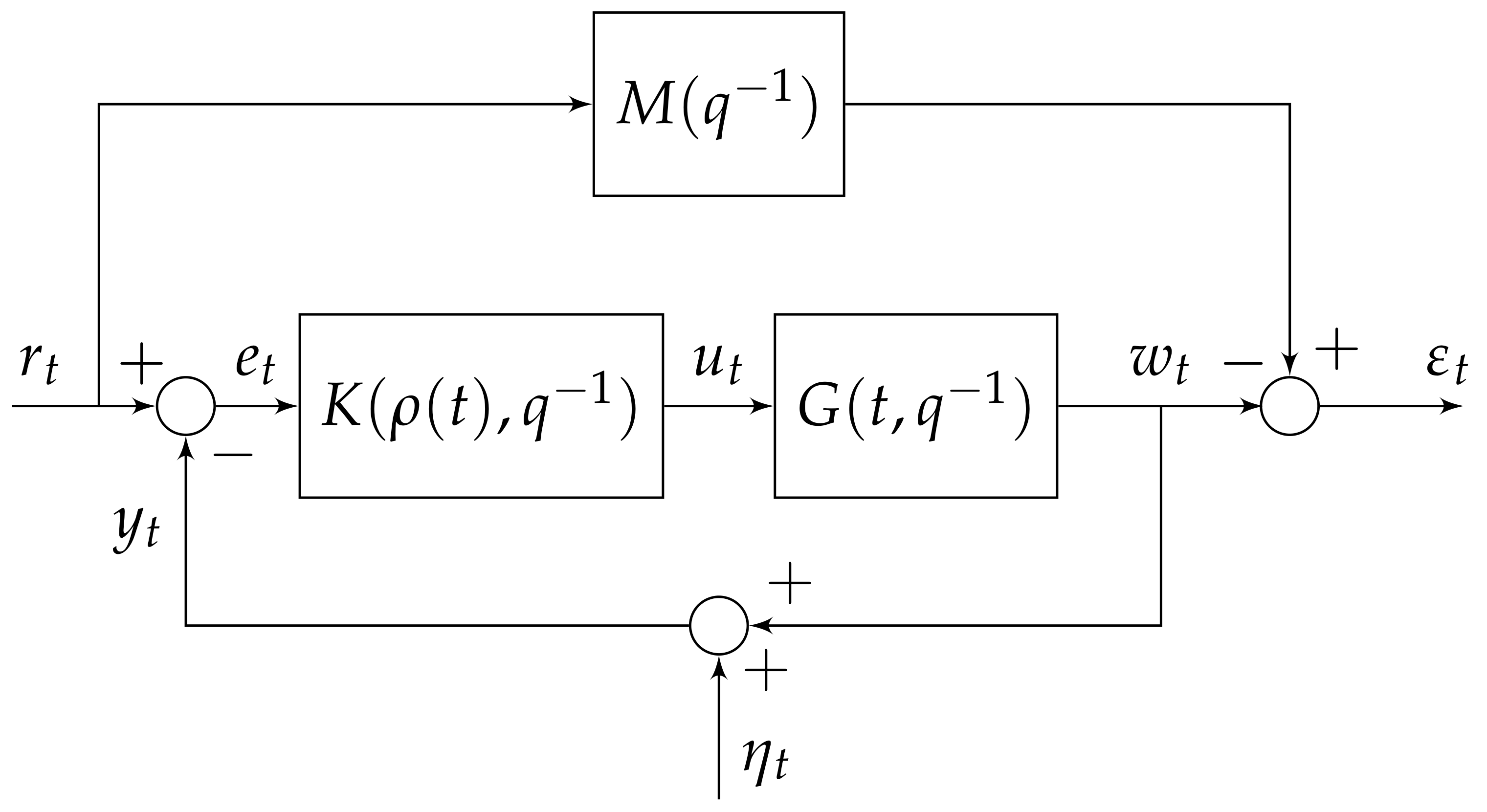
Let us consider the discrete-time single-input single-output (SISO) feedback control scheme depicted in Figure 1, where denotes the backward shift operator (i.e., ), and is the transfer function of a given linear time invariant (LTI) reference model that describes the desired closed-loop behaviour of the feedback control system to be designed.
The plant to be controlled is described by a SISO LTV system defined by the following linear difference equation
where is the plant input (controller output) and is the noise free output signal, while and are time-varying polynomials described by
where . The parameters and vary according to
and
where and are unknown parameter variations between two consecutive generic time instants and t.
Let be the noise-corrupted measurement of ,
Measurement uncertainty is known to range within given bound , more precisely
Let us now introduce the following two assumptions.
Assumption 1.
The transfer function is assumed to be stable and minimum phase .
Assumption 2.
The transfer function is assumed to be minimal .
Assumption 2 is equivalent to say that the system is completely controllable and observable.
The controller is a SISO LTV system described by the following equations
where is the difference between the reference signal and the noise-corrupted output , i.e.,
and time-varying polynomials and are represented as
where we assume that .
As same as the plant, the parameters of the controller and are assumed to vary according to
and
where and are the controller’s parameter variations between two successive time instants and t. The parameter variation vector is defined as follows,
where . We assume that is unknown, but bounded. More specifically, we assume that belongs to the the following time-varying set:
where , , due to the structure of the addressed problem, are unknown variation bounds. This point will be addressed in the next section.
The aim of this work is to estimate, at each time instant t, the parameter vector , characterizing the controller , defined as
without explicitly taking into account any information about the plant, neither its structure or how the parameters vary, i.e., Equations (1)–(5). This is due to the fact that we are considering a model-free setting for the plant, as we can not rely on having such information, and we only use the input-output data from the plant to design .
At this point, the data-driven control problem for LTV systems, considered in this paper, can be stated as follows.
Problem 1
(Adaptive Data-Driven Controller Design). The problem addressed in this paper is to design a time-varying controller such that the the closed loop transfer function , at each time step t, given by
matches, as close as possible, that of the assigned reference model , under the assumption that the plant transfer function is unknown. In other words, we want to find a controller that makes the output matching error signal , defined as:
as close as possible to zero.
Please note, in order to simplify notation, we drop the backward shift operator from all equations presented in the remainder of this paper.
3. Adaptive DDC for LTV Systems in the Set-Membership Framework
In this section, we address the formulation of the adaptive data-driven control design problem, as described in Problem 1.
First let us introduce the time-varying feasible controller set (FCS), which is inspired by the feasible parameter set (FPS) for LTV systems proposed in [26] and the FCS definition for LTI controllers presented in [23]. The time-varying FCS, for the case of LTV systems, is defined as follows.
Definition 1.
[Time-Varying Feasible Controller Set]
At a generic time t, the feasible controller set (FCS) is defined as the set of all controllers belonging to a given model class such that for each controller in this set there exists at least one noise sequence and parameter variations , , such that the difference between the reference model output and that of the closed-loop system
From Definition 1, the time-varying FCS can be described as:
As it can be clearly seen from the set , the controller class is parametrized by , hence we can replace the time-varying set with the time-varying feasible controller parameter set which is defined as follows.
Definition 2.
[Time-Varying Feasible Controller Parameter Set]
The feasible controller parameter set (FCPS), at a generic time t, is defined as the set of all the controller parameters such that .
On the basis of Definition 2, we now state the following result.
Result 1.
Structure of the Feasible Controller Parameter Set
At a generic time instant t, the feasible controller parameter set (FCPS) for the time-varying controller , is defined as
where,
and are the parameters of an initial controller that stabilizes the plant.
Proof.
Starting from the time-varying FCS, as in Definition 1, the output matching error signal Equation (18) can be written as:
The closed-loop system’s output , which is the unknown plant’s output, is equal to:
or equivalently,
The term () can be written as,
where is the sensitivity function.
Based on the approach presented in [27], we introduce the following approximation,
where is the ideal controller and follows the same definition as in [23].
Finally, dividing both sides of Equation (30) by and multiplying by leads to:
which can be equivalently rewritten as,
where,
□
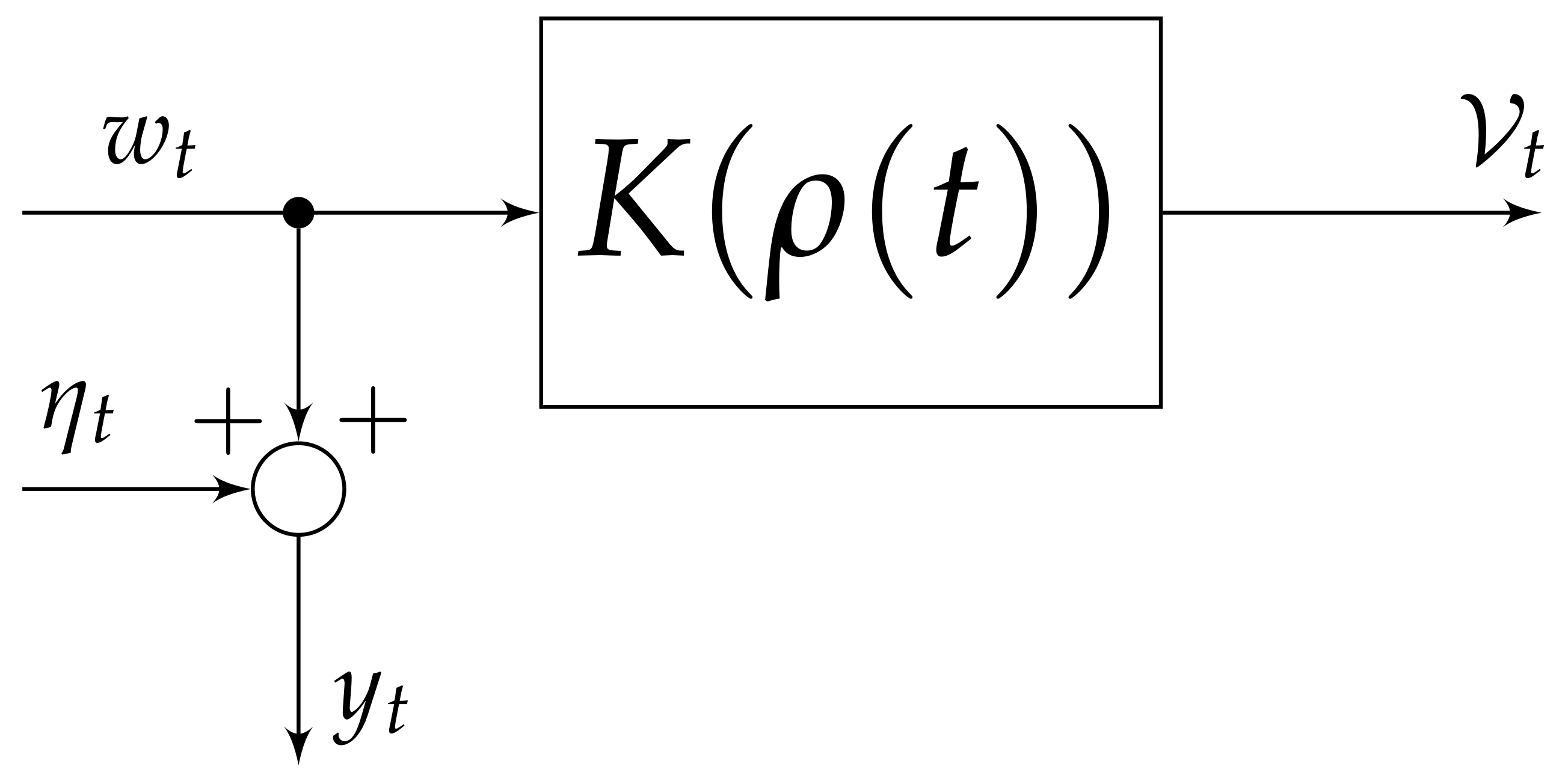
A block diagram description of Equation (32), characterizing the FCPS in (21), is given in Figure 2. This figure shows that by collecting from the closed-loop system, shown in Figure 1, the noise corrupted output measurements and the control input , we can design the adaptive controller by solving a suitable optimization problem as will be described in the next section.
As given from Definition 2, the FCPS contains all the parameters such that . In practice, however, we need to pick just a single point from the FCPS to design the controller to be implemented in the feedback control scheme as in Figure 1. As it can be clearly seen from the set in (21), the FCPS is characterized by the unknown variation bounds , . Therefore, in order to design we need to compute these variation bounds. In the next section we will address the problem of finding a single point controller, at each time instant t, in the FCPS that corresponds to the minimum value bounding the variation on all parameters .
4. Parameter Variation Bounds Computation
In this section, we propose an algorithm for computing the minimum variation value that bounds all parameters .
First, let us introduce the following time-dependant parameters variation vector
where characterizes the time-varying set in (15). In order to compute the minimum parameter variation vector we need to solve the following multi-objective optimization problem
Multi-objective optimization (MOO) problems are those that involve more than one objective function to be optimized simultaneously. Several approaches tackling MOO problems are present in the literature (see, e.g., [28,29,30,31]). All of these techniques do not return the exact solution for each objective function, but rather a trade-off between all of them by approximating a set of Pareto optimal solutions. In the problem addressed in this section, we want to know the variation bound for each of the controller parameters, but the solution of the multi-objective optimization problem (35) will return the best candidates that minimize all objective functions together, which may not necessarily be the true value for the variation bounds. On the other hand, another crucial point worth highlighting, is the fact that the computation complexity of solving MOO can not be applied in the adaptive scheme considered in this paper.
In the following formulation, we will consider the case of computing a single variation bound, denoted as hereinafter, that represents the minimum variation bounding all . In other words, we want to find a single point controller that corresponds to the minimum variation bound . We can generically formulate the problem mathematically as:
where,
The following result shows that (36) can be written as a constrained polynomial optimization problem.
Result 2.
Computation of
The controller parameters , corresponding to the minimum variation bound , can be computed solving the following optimization problem:
where .
Problem (38) is a nonconvex polynomial optimization problem due to the presence of bilinear terms in the equation , i.e., the controller parameters are multiplied by samples of the unknown measurement noise. The global optimal solution of problem (38) can be approximated by means of semidefinite programming relaxation techniques, see, e.g., [32,33,34]. However these methods require huge computational efforts and memory resources, and hence can not be applied in the considered adaptive control scheme. In the next section, we propose a convex relaxation approach which allows us to rewrite optimization problem (38) as a linear problem starting from the results recently presented in [25].
5. A Convex Relaxation Approach
In this section, we propose a convex relaxation approach, which allows us to rewrite the nonconvex optimization problem (38) as an equivalent linear problem. The main idea is based on the work recently proposed in [25], where we rely on the concept of McCormick envelopes [35] to relax the original problem to an equivalent convex one.
Let us first rewrite Equation (32) as follows
Now to eliminate the bilinear terms in (39), we introduce the following variables,
allowing us to write (39) as
Now direct application of the approach presented in [25] allows us to state the following result in order to bound .
Result 3.
Upper and lower bounds on
Based on the concept of McCormick envelopes, , , satisfies the following set of inequalities
Bounds and are given by
where are the estimates at time .
As it can be clearly observed from Result 3, by substituting (46) and (47) into inequalities (42)–(45), we once again encounter bilinear terms due to the multiplication of the unknown variation bounds with the noise samples, i.e., . In the next result, we show that (42)–(45) can be written as equivalent linear inequalities.
Since the proof for all four inequalities in Result 4 is the same, for simplicity we will only prove that inequality (48) is equivalent to (42).
Proof.
Since , , are unknown but bounded according to (7), Equation (52) can be rewritten equivalently as:
where is a known value (estimate at time ), and upper bound on the variation is greater than or equal to zero, i.e., , .
□
Remark 1.
For LTV systems, in most cases it is safe to assume that all variation bounds are strictly greater than zero, i.e., . However, there can be some cases where this statement is not true, e.g., a PI controller, hence assuming that assures the possibility of having a more general setting. Furthermore, one other case where this setting is useful is when the plant to be controlled is an LTI one, which implies by definition that variations on the controller parameters, after a transient state, are equal to zero.
At this point we are in a position to state the main result of the paper.
Result 5.
Computation ofby means of Linear Programming (LP)
The controller parameters can be computed by solving the following linear program:
where the decision variables are the unknown parameters , and the variables , .
6. Simulation Examples
The effectiveness of the proposed approach is shown by means of a two simulation examples. Computations are performed on an Intel Core i7-10510U @ 1.80 GHz computer with 16 GB RAM, using the IBM ILOG CPLEX optimizer under Matlab R2018b.
6.1. Example 1
In this first example we demonstrate the parameter tracking properties of the proposed adaptive control design scheme by considering an example where the structure of the ideal controller, referred to as hereinafter, is known.
Let us consider the following second order LTV system,
where the coefficients characterizing vary according to,
The assigned reference model, describing the desired closed-loop behaviour, has the following transfer function
and the model-based ideal controller , computed algebraically through the model-matching Equation (18) (where ) is given by,
The sampling time is equal to 0.005 s.
The reference signal is a random sequence uniformly distributed between . The plant output is corrupted by a random additive noise , uniformly distributed in the range . The error bound is chosen such that the Signal to Noise Ratio on the output , defined as:
is equal to 33 dB.
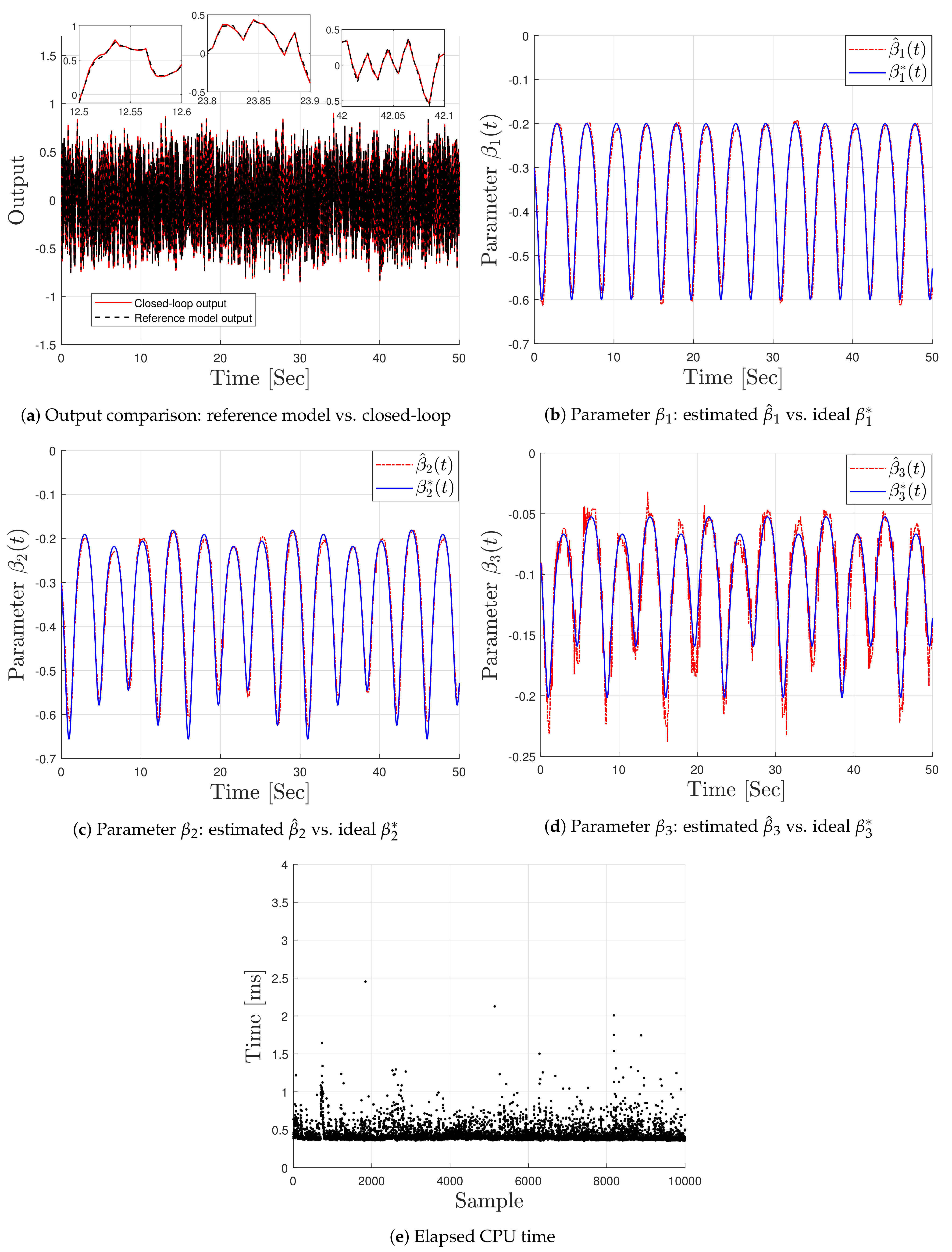
Figure 3a shows the tracking performance of the closed-loop system, compared to that of the reference model. Figure 3b–d show the computed controller parameters alongside the ideal coefficients that are calculated algebraically according to Equation (57). As it can be seen from these figures, parameters and have a time varying profile that is not entirely linear. Nevertheless, the parameters computed, solving optimization problem (54), are still able to track the variations in the system, and provide overall good performance. In Figure 3e we can see the average CPU time to compute the controller at each time step, which is less than 1 ms in most instances.
Remark 2.
The aim behind this example is to showcase how the controller computed by solving optimization problem (54) compares to the ideal model-based controller . For this reason the structure for has been chosen as a proper transfer function as shown in (57). However, in general the transfer function of the ideal controller could be highly complex, and in some cases not implementable, i.e., non proper, as it will depend on the choice of the reference model M, and the model structure of the plant to be controlled. Since the aim of the DDC approach presented in this work is to compute without explicitly having any knowledge about the plant, the next example we will consider the case where we assume not to know the structure of .
6.2. Example 2
The plant to be controlled, which is assumed to be unknown, is a third order LTV system described by the following transfer function,
where,
and is a fixed parameter, while the reference model has the following transfer function
The sampling time is set equal to 0.01 s.
For this example we consider a square wave reference with an amplitude equal to one and frequency 0.2 rad/s. The true plant output is corrupted by random additive noise, uniformly distributed between . The error bound is chosen such that the Signal to Noise Ratio on the output, calculated according to Equation (58), is equal to dB.
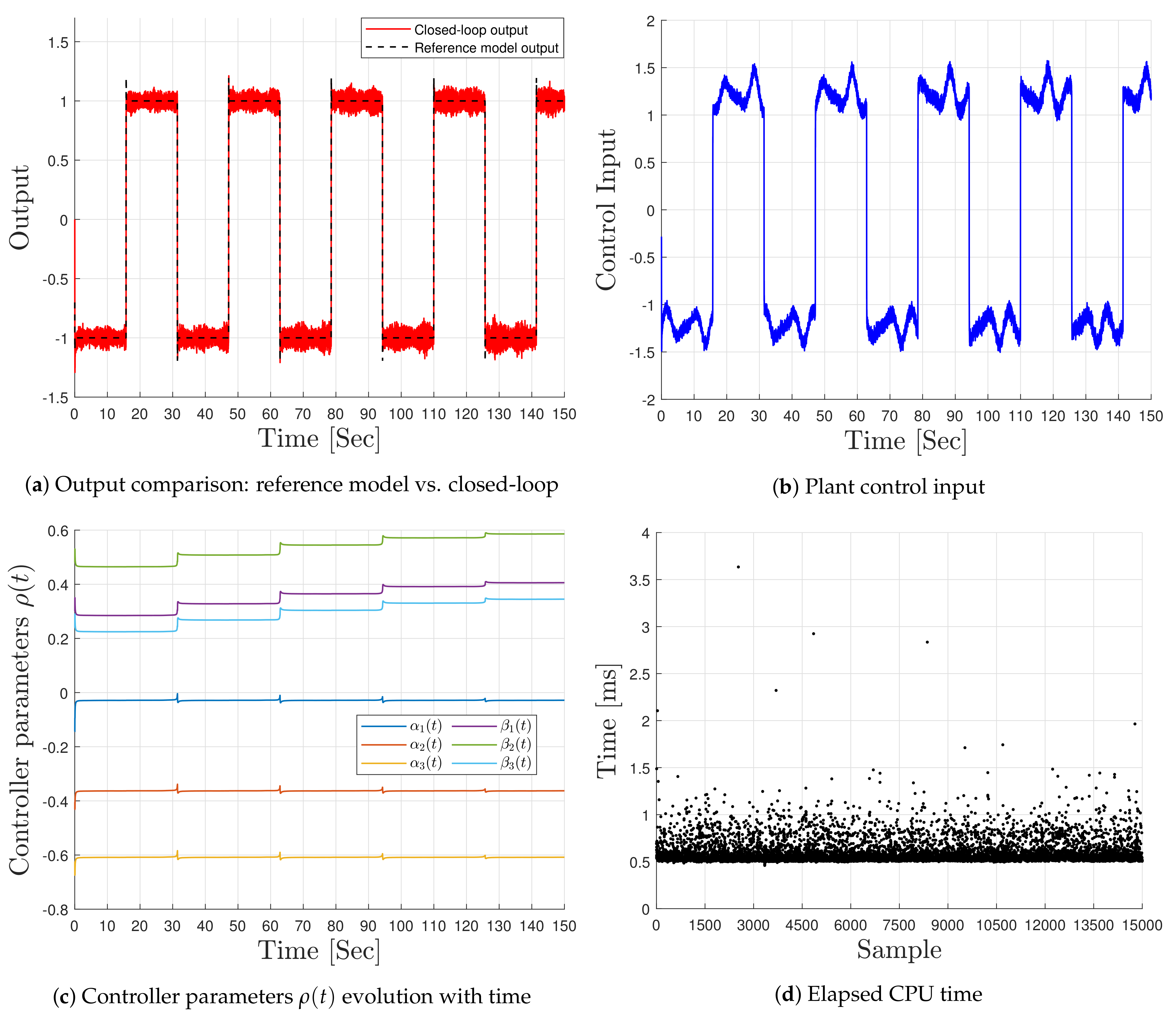
In Figure 4a, we can see a comparison between the output of assigned reference model and the performance of the designed feedback control system. The controller structure is selected as:
which is the one that provides the best trade-off in terms of performance while maintaining low complexity. It is worth mentioning that higher order controllers do not provide much improvement in performance, and in some cases lead to unwanted behaviours. In Figure 4b we can see the control input and how it is adjusting to cope up with the variations in the plant. The adaptive controller parameters are reported in Figure 4c. The average elapsed CPU time to compute the controller parameters, at each sampling instant is less than 1.5 ms as can be seen in Figure 4d. This strongly motivates the validity of this approach, as it is able to track the desired reference while maintaining very low computation time.
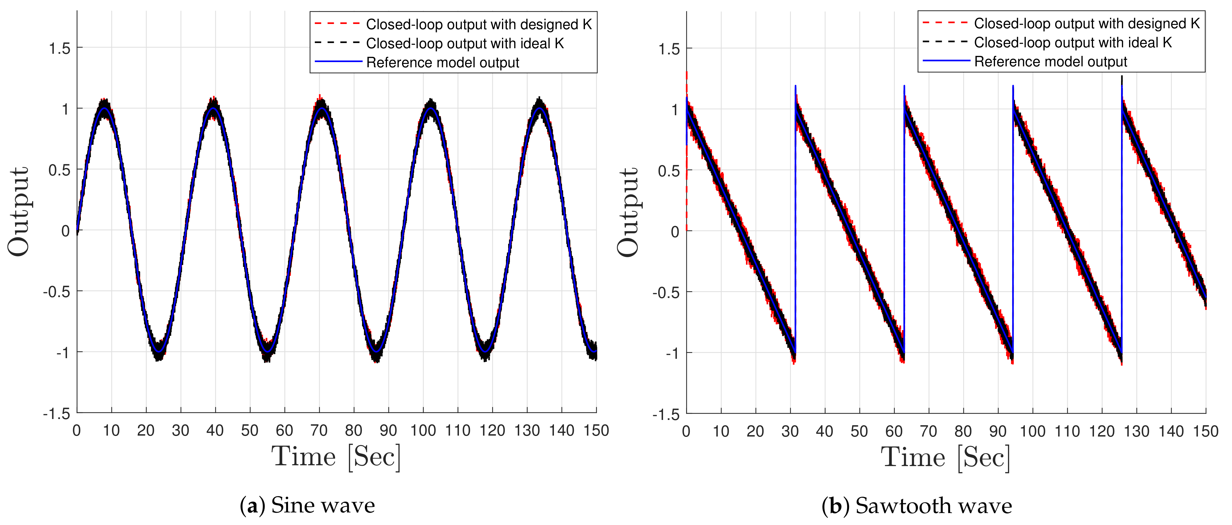
In order to further analyse the performance of the designed feedback control system, we compare it against the output of the loop which includes the ideal controller given through the model-matching equation,
In Figure 5, we compare the outputs of the closed-loop system with the ideal controller , calculated algebraically, and the system with . We use two reference signals for performing the comparison; sine and sawtooth waves having the same amplitude and frequency as the square wave mentioned above. From the figure, it can be noticed that the overall performance of both control loops is quite similar, except for a relatively small additional error appearing in the loop with .
7. Conclusions and Future Works
An adaptive data-driven control approach for linear time varying systems is presented. First, through a model-matching scheme, we formulate the the controller design problem as a suitable polynomial optimization problem in the set-membership identification framework. Characterizing the variation on the controller parameters, we then propose a reformulation to compute a single point controller that corresponds to the minimum upper bound on the parameters variation. A convex relaxation approach, based on McCormick envelopes, is proposed to solve the controller design problem by means of linear programming. Effectiveness of the proposed approach is shown by means of two simulation examples.
The work presented in this paper sets the basic foundations for the problem of designing adaptive controllers for LTV systems using set-membership identification techniques. In future works, activities will be devoted towards the following:
- Deriving conditions that assure stability of the designed feedback control system, allowing us to consider the problem of controlling unstable, as well as non-minimum phase, systems.
- Extension of the results to the control of nonlinear systems.
- Extending the approach presented in this paper to the control of multivariable LTV systems.
Funding
This research received no external funding.
Institutional Review Board Statement
Not applicable.
Informed Consent Statement
Not applicable.
Data Availability Statement
Not applicable.
Conflicts of Interest
The author declares no conflict of interest.
Abbreviations
The following abbreviations are used in this manuscript:
| DDC | Data-driven control |
| LTV | Linear time varying |
| LTI | Linear time invariant |
| SISO | Single-input single-output |
| FCS | Feasible controller set |
| FCPS | Feasible controller parameter set |
| FPS | Feasible parameter set |
| MOO | Multi-objective optimization |
| LB | Lower bound |
| UB | Upper bound |
| LP | Linear programming |
References
- Tsakalis, K.; Ioannou, P. Adaptive control of linear time-varying plants. Automatica 1987, 23, 459–468. [Google Scholar] [CrossRef]
- Meyn, S.; Brown, L. Model reference adaptive control of time varying and stochastic systems. IEEE Trans. Autom. Control 1993, 38, 1738–1753. [Google Scholar] [CrossRef]
- Koh, K.; Kamen, E. Robust Indirect Adaptive Control of Linear Time-Varying Systems. In Proceedings of the 1988 American Control Conference, Atlanta, GA, USA, 15–17 June 1988; pp. 777–778. [Google Scholar]
- Kreisselmeier, G. Adaptive control of a class of slowly time-varying plants. Syst. Control Lett. 1986, 8, 97–103. [Google Scholar] [CrossRef]
- Li, Y.; Chen, H.F. Robust adaptive pole placement for linear time-varying systems. IEEE Trans. Autom. Control 1996, 41, 714–719. [Google Scholar]
- Miller, D. A new approach to model reference adaptive control. IEEE Trans. Autom. Control 2003, 48, 743–757. [Google Scholar] [CrossRef]
- Bobtsov, A.A.; Nagovitsina, A.G. Adaptive output control of linear time-varying systems. In Proceedings of the 9th IFAC Workshop on Adaptation and Learning in Control and Signal Processing, Saint Petersburg, Russia, 29–31 August 2007; Volume 40, pp. 334–341. [Google Scholar]
- Hjalmarsson, H.; Gevers, M.; Gunnarsson, S.; Lequin, O. Iterative feedback tuning: Theory and applications. IEEE Control Syst. Mag. 1998, 18, 26–41. [Google Scholar]
- Campi, M.; Lecchini, A.; Savaresi, S. Virtual reference feedback tuning: A direct method for the design of feedback controllers. Automatica 2002, 38, 1337–1346. [Google Scholar] [CrossRef] [Green Version]
- Campi, M.; Lecchini, A.; Savaresi, S. An Application of the Virtual Reference Feedback Tuning Method to a Benchmark Problem. Eur. J. Control 2003, 9, 66–76. [Google Scholar] [CrossRef]
- Karimi, A.; van Heusden, K.; Bonvin, D. Non-iterative data-driven controller tuning using the correlation approach. In Proceedings of the 2007 European Control Conference (ECC), Kos, Greece, 2–5 July 2007; pp. 5189–5195. [Google Scholar]
- Safonov, M.G.; Tsao, T.C. The unfalsified control concept: A direct path from experiment to controller. In Feedback Control, Nonlinear Systems, and Complexity; Francis, B.A., Tannenbaum, A.R., Eds.; Springer: Berlin/Heidelberg, Germany, 1995; pp. 196–214. [Google Scholar]
- De Persis, C.; Tesi, P. Formulas for Data-Driven Control: Stabilization, Optimality, and Robustness. IEEE Trans. Autom. Control 2020, 65, 909–924. [Google Scholar] [CrossRef] [Green Version]
- Hou, Z.S.; Wang, Z. From model-based control to data-driven control: Survey, classification and perspective. Inf. Sci. 2013, 235, 3–35. [Google Scholar] [CrossRef]
- Bazanella, A.; Campestrini, L.; Eckhard, D. Data-driven Controller Design: The H2 Approach; Springer Science & Business Media: Berlin, Germany, 2012. [Google Scholar]
- Campestrini, L.; Eckhard, D.; Sanfelice Bazanella, A.; Gevers, M. Data-driven model reference control design by prediction error identification. J. Frankl. Inst. 2017, 354, 2628–2647. [Google Scholar] [CrossRef]
- Radac, M.B.; Precup, R.E. Data-Driven Model-Free Tracking Reinforcement Learning Control with VRFT-based Adaptive Actor-Critic. Appl. Sci. 2019, 9, 1807. [Google Scholar] [CrossRef] [Green Version]
- Karimi, A.; Kammer, C. A data-driven approach to robust control of multivariable systems by convex optimization. Automatica 2017, 85, 227–233. [Google Scholar] [CrossRef] [Green Version]
- Nicoletti, A.; Martino, M.; Karimi, A. A data-driven approach to power converter control via convex optimization. In Proceedings of the 2017 IEEE Conference on Control Technology and Applications (CCTA), Maui, HI, USA, 27–30 August 2017; pp. 1466–1471. [Google Scholar]
- Nicoletti, A.; Martino, M.; Karimi, A. A data-driven approach to model-reference control with applications to particle accelerator power converters. Control Eng. Pract. 2019, 83, 11–20. [Google Scholar] [CrossRef]
- Makarem, S.; Delibas, B.; Koc, B. Data-Driven Tuning of PID Controlled Piezoelectric Ultrasonic Motor. Actuators 2021, 10, 148. [Google Scholar] [CrossRef]
- Berberich, J.; Köhler, J.; Müller, M.A.; Allgöwer, F. Data-Driven Model Predictive Control With Stability and Robustness Guarantees. IEEE Trans. Autom. Control 2021, 66, 1702–1717. [Google Scholar] [CrossRef]
- Cerone, V.; Regruto, D.; Abuabiah, M. Direct data-driven control design through set-membership errors-in-variables identification techniques. In Proceedings of the 2017 American Control Conference (ACC), Seattle, WA, USA, 24–26 May 2017; pp. 388–393. [Google Scholar]
- Cerone, V.; Regruto, D.; Abuabiah, M. A set-membership approach to direct data-driven control design for SISO non-minimum phase plants. In Proceedings of the 2017 IEEE 56th Annual Conference on Decision and Control (CDC), Melbourne, VIC, Australia, 12–15 December 2017; pp. 1284–1290. [Google Scholar]
- Fosson, S.M.; Regruto, D.; Abdalla, T.; Salam, A. A convex optimization approach to online set-membership EIV identification of LTV systems. arXiv 2021, arXiv:2107.01714. [Google Scholar]
- Cerone, V.; Fosson, S.M.; Regruto, D.; Abdalla, T. A recursive approach for set-membership EIV identification of LTV systems with bounded variation. In Proceedings of the 2020 59th IEEE Conference on Decision and Control (CDC), Jeju, Korea, 14–18 December 2020; pp. 3951–3956. [Google Scholar]
- van Heusden, K.; Karimi, A.; Bonvin, D. Data-driven model reference control with asymptotically guaranteed stability. Int. J. Adapt. Control Signal Process. 2011, 25, 331–351. [Google Scholar] [CrossRef] [Green Version]
- Miettinen, K. Nonlinear Multiobjective Optimization; International Series in Operations Research & Management Science; Springer US: Berlin, Germany, 2012. [Google Scholar]
- Wierzbicki, A.P. A mathematical basis for satisficing decision making. Math. Model. 1982, 3, 391–405. [Google Scholar] [CrossRef] [Green Version]
- Branke, J.; Branke, J.; Deb, K.; Miettinen, K.; Slowiński, R. Multiobjective Optimization: Interactive and Evolutionary Approaches; Genetic Algorithms and Evolutionary Computation; Springer: Berlin, Germany, 2008. [Google Scholar]
- Coello, C.; Lamont, G.; van Veldhuizen, D. Evolutionary Algorithms for Solving Multi-Objective Problems; Genetic and Evolutionary Computation; Springer US: Berlin, Germany, 2007. [Google Scholar]
- Lasserre, J.B. Global Optimization with Polynomials and the Problem of Moments. SIAM J. Optim. 2001, 11, 796–817. [Google Scholar] [CrossRef]
- Chesi, G.; Garulli, A.; Tesi, A.; Vicino, A. Solving quadratic distance problems: An LMI-based approach. IEEE Trans. Autom. Control 2003, 48, 200–212. [Google Scholar] [CrossRef]
- Parrilo, P. Semidefinite Programming Relaxations for Semialgebraic Problems. Math. Program. Ser. B 2003, 96, 293–320. [Google Scholar] [CrossRef]
- McCormick, G.P. Computability of global solutions to factorable nonconvex programs: Part I—Convex underestimating problems. Math. Program. 1976, 10, 147–175. [Google Scholar] [CrossRef]
Figure 1.
Adaptive data-driven control closed-loop model-matching scheme.

Figure 2.
Adaptive data-driven control: design scheme.

Figure 3.
Example 1: Performance of the designed closed-loop feedback control system.

Figure 4.
Example 2: Performance of the designed closed-loop feedback control system.

Figure 5.
Example 2: Comparison between the closed-loop outputs: ideal controller K* vs. designed controller K(ρ(t)).
Figure 5.
Example 2: Comparison between the closed-loop outputs: ideal controller K* vs. designed controller K(ρ(t)).

Publisher’s Note: MDPI stays neutral with regard to jurisdictional claims in published maps and institutional affiliations. |
© 2021 by the author. Licensee MDPI, Basel, Switzerland. This article is an open access article distributed under the terms and conditions of the Creative Commons Attribution (CC BY) license (https://creativecommons.org/licenses/by/4.0/).
Share and Cite
MDPI and ACS Style
Abdalla, T. Adaptive Data-Driven Control for Linear Time Varying Systems. Machines 2021, 9, 167. https://doi.org/10.3390/machines9080167
AMA Style
Abdalla T. Adaptive Data-Driven Control for Linear Time Varying Systems. Machines. 2021; 9(8):167. https://doi.org/10.3390/machines9080167
Chicago/Turabian StyleAbdalla, Talal. 2021. "Adaptive Data-Driven Control for Linear Time Varying Systems" Machines 9, no. 8: 167. https://doi.org/10.3390/machines9080167
Note that from the first issue of 2016, this journal uses article numbers instead of page numbers. See further details here.