1. Introduction
In mechatronic applications the choice of motor and transmission must take into account two main issues concerning the motor, its thermal problem and its torque peak problem, to be considered in parallel. As for the latter, during the working cycle, the drive system must often exert considerable torque peaks to balance high resistant and inertia loads acting in small time ranges. These torque peaks must be allowed by the dynamic operating range of the drive system.
The interposition of the transmission between motor and load makes the problem more complex and interesting for many reasons. First, the transmission ratio reduces the motor speed and amplifies the motor torque on load side. Second, the direct and inverse transmission efficiencies, denoted by and , respectively, modify the required motor torque. Third, sometimes the transmission inertia on motor side and on load side significantly increase the inertia torque. Fourth, the transmission speed limit on motor side and the torque limit on load side impose two constraints that must be respected.
The complexity of the problem requires the simultaneous choice of drive system and transmission according to different methods described in the technical literature.
Some papers regard the drive train optimization for industrial robots, for which a concurrent design approach is required in order to take into consideration the reciprocal effect of the different drive trains. Both the thermal problem and the torque peak problem of the motor are taken into account. The optimization requires a complete model of the robot and an adequate model of transmission and drive system. The optimal motor-reducer couple is found by minimizing a single or multi-objective criterion. A multi-objective optimization permits a good compromise among different requirements regarding both the general characteristics of the machine (cost, weight etc.) and its performances, as shown in the following works. Roos et al. [
1] compared the drive system-transmission couples able to perform the reference task by means of suitable diagrams for the minimization of the different objective functions. Petterson et al. [
2] considered a model of the motor in which all the parameters are continuous functions of the design variables (length and radius of the motor), while the transmission parameters depend on a discrete number of its size. The optimization results are the motors and transmissions that minimize the global cost while respect the performance requirements. Zhou et al. [
3] studied the optimization of the drive trains of a light-weight robot. Motors and transmissions, taken from a limited catalog, are simultaneously optimized for the different axes. Ge et al. [
4] carried out the optimal choice of motors and transmissions among available components by means of dynamic optimization, with an objective function made up of working efficiency and natural frequency. Padilla-Garcia et al. [
5] introduced an electro-mechanical model of the motors that allows the designer to obtain the dynamics of the robot. The transmissions are assigned. A genetic algorithm allows the choice of off the shelf servomotors and the tuning of the control gains, with an objective function that minimizes tracking error, global weight of the motors and energy consumption.
More recent papers concern mobile robots and/or robots with compliant actuators with particular reference to the energy efficiency. For non-linear dynamics, Nasiri et al. [
6], proposed to adapt non-linear compliances in order to minimize a cyclic energy consumption. For robots interacting with men, Verstraten et al. [
7] analyzed the effect of series elastic actuators and parallel elastic actuators for an often-relevant minimization of the power peak and the energy consumption. Haddadin et al. [
8] compared motors with elastic joints with motors with rigid joints, both reaching the same maximum speed, in order to find the mass decrease of the first solution. For robot applications, Saerens et al. [
9] studied scaling laws for different transmission types in view of a multi-variable optimization, and found the influence of diameter, length, transmission ratio and number of stages on the maximum continuous output torque and the generalized inertia on load side. Saerens et al. [
10] conducted a similar study for different types of springs for compliant actuators in view of their energy storage capacity. In all these works, the efficiency of the transmission is considered in an approximate way.
Some papers concern the selection of drive system and transmission when the motor must be modelized with an internal viscous torque due to the iron losses. Particular attention is paid to the energy efficiency. In particular, Rezazadeh et al. [
11] proposed a method for the choice of the motor-transmission couple based on the minimization of the total energy for a given reference task and on the minimization of the bandwidth as a second objective function. For a mobile robot, Verstraten et al. [
12] proposed a model of motor and transmission in order to evaluate the mechanical and electrical energy losses, and provided a series of recommendations in this regard. Verstraten et al. [
13] compared different models for the prediction of the energy consumption of a DC motor-transmission couple, and underlined the relevance of the power flow direction in this regard. Bartlett et al. [
14] proposed a method for the optimal choice of the transmission ratio in terms of rms motor torque and rms electrical power, taking into account the saturation and the thermal limits of the drive system.
In a more classical approach, a single axis is taken into account, and there is a distinction between two phases. A first feasibility phase allows the designer to find all the admissible drive system-transmission pairs with respect to a specified reference task; it should be followed by an optimization phase, which allows the designer to find, among those admissible, the drive system-transmission couple that minimizes additional criteria. Normally, these papers stop at the first phase. The present paper adopts this approach.
Some papers [
15,
16,
17,
18] take into account the complete set of the motor characteristics, whereas they only consider the main parameter of the speed reducer, i.e., the transmission ratio
τ. Sometimes, these papers only deal with the motor thermal problem, other times only with the torque peak problem and other times with both of them. Nevertheless, all the systems must be further checked, taking into consideration the complete set of the transmission characteristics: hence, only after this second step, the admissibility of the drive system-transmission couple can be ensured.
Other papers [
19,
20,
21,
22,
23,
24,
25] take into account the reducer efficiency from the outset.
The method introduced by Van de Straete [
16] is extended by Giberti et al. [
19,
20]. They considered the motor thermal problem and both the direct and inverse transmission efficiency. However, on the one hand, these parameters are constant, and on the other hand, during the reference task, the power flow through the speed reducer is unidirectional, either direct or inverse. With this approach, some admissible drive system-transmission couples can be improperly excluded.
Generally, in mechatronic applications, the power flow through the reducer changes its direction, generating an alternation of the direct and inverse transmission efficiency; just think of the inertia forces of the load. In general, this condition increases the set of the admissible motor–transmission couples. Cusimano [
21,
22] introduced the alternation of the mechanical power flow through the transmission. He studied the choice of the motor-transmission couple with reference to a rectangular dynamic operating range.
The case of a non-rectangular dynamic operating range of the drive system is dealt with by Cusimano [
23,
24]. The first work shows how the choice method proposed in [
16,
19] can be applied to this case, whereas paper [
24] presents a new and more complete approach.
With reference to the motor thermal problem, Cusimano et al. [
25] proposed a method in which each candidate transmission is singularly taken into consideration. The first step is to check if it is able to move the load according to its speed and torque limits, i.e., if it is admissible. Then, for each admissible transmission, the second step is to find all the drive systems that can be coupled with it in order to execute the reference task from the point of view of the thermal problem of the motor. Thus, it is possible to find all the motors that can be coupled with a given transmission without the need of a further check. The motors taken into account present a nearly horizontal limit curve of their continuous duty operating range S1.
The present work deals with the problem of the torque peak of the motor, and its rationale is to consider the candidate transmissions one by one; hence, all their parameters are known from the outset. Following a path similar to that traced in [
25], not only all the drive system parameters but also all the transmission parameters are taken into account from the beginning: therefore, all the candidate drive systems that can be coupled with each candidate transmission are definitively determined, without the need of a further check. To this aim, a completely automated procedure is used. Furthermore, the work presents the guidelines to draw new diagrams that allow the designer to compare the admissible drive system-transmission pairs. Initially the authors consider motors with a nearly horizontal limit curve of their continuous duty operating range and a horizontal limit curve of their dynamic operating range. Afterwards, they also consider motors with a different shape of these operating ranges.
In particular, in this paper,
Section 2 explains the load specifications and indicates the inequalities due to the constraints regarding both transmission and motor.
Section 3 considers a given speed reducer and checks if it must be excluded according to the corresponding inequalities; otherwise, it introduces an automated procedure to find the admissible drive system-transmission couples when the dynamic operating range can be considered rectangular. For each admissible speed reducer,
Section 4 introduces new diagrams in order to find and compare the drive systems that are able to exert the required torque peaks of the motor. In
Section 5, an industrial case study is analyzed.
Section 6 solves the torque peak problem for drive systems that show a non-rectangular dynamic operating range: for many of them, the procedure is similar to that applied when the dynamic operating range is rectangular; for the remaining ones, a more complex method is explained.
Section 7 shows how the proposed procedure can be applied to motors with an internal viscous torque.
Section 8 discusses the conclusions.
2. Specifications
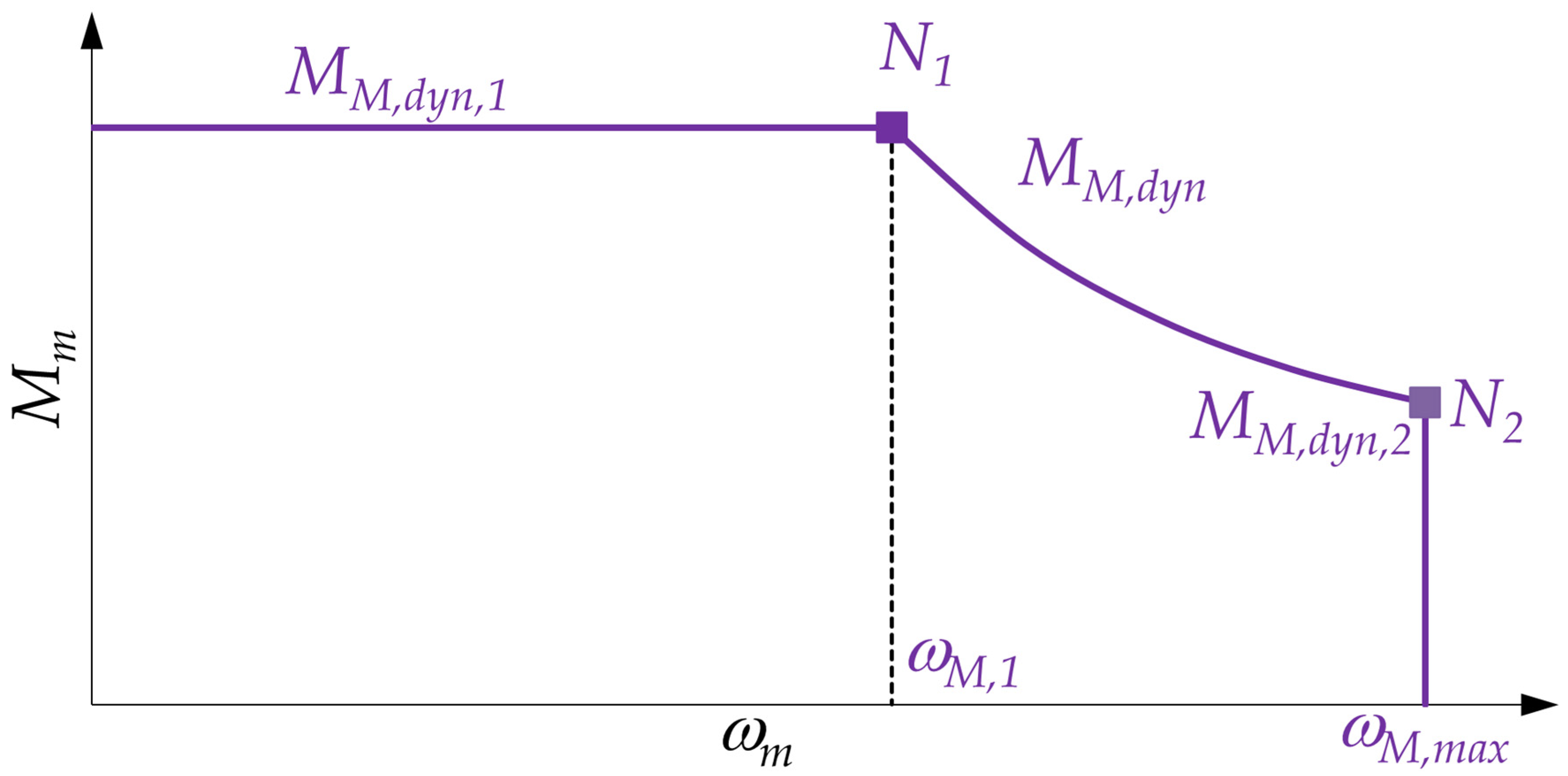
Figure 1 shows the first quadrant of the dynamic operating range of a permanent magnet brushless motor.
Denoting the motor torque by Mm and its speed by ωm, in the ωm-Mm plane, the dynamic operating range is limited by the motor maximum speed ωM,max and by a variable torque , due to the electronic drive feeding the motor. As far as speed ωM,1, at which the voltage saturates, is constant. Beyond ωM,1, there is a descending profile of At a given speed ωm, if the required motor torque Mm should be higher than the electronic drive would not allow the motor to exert it, so that the machine would not work properly: this is the torque peak problem.
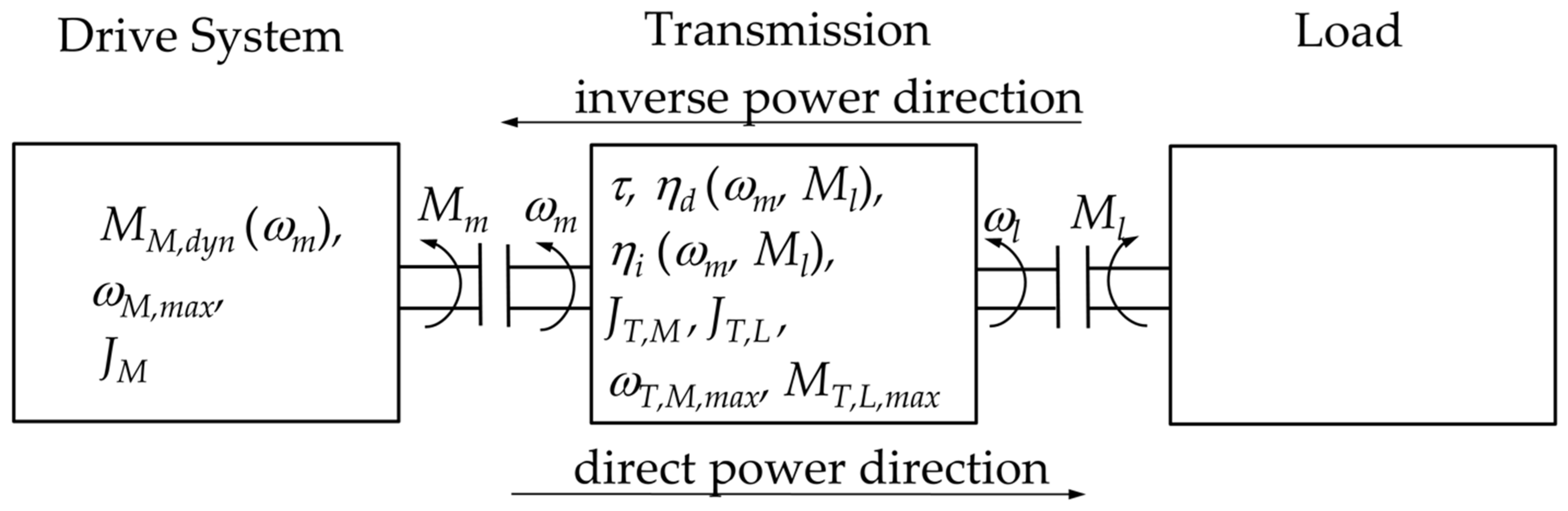
Figure 2 shows the scheme of a machine. For the choice of motor and transmission suitable to move a joint only the corresponding degree of freedom of the machine is taken into consideration, whereas the effects of other degrees of freedom are included in the load torque
Ml exerted on the joint. This torque includes both inertia and resistant loads.
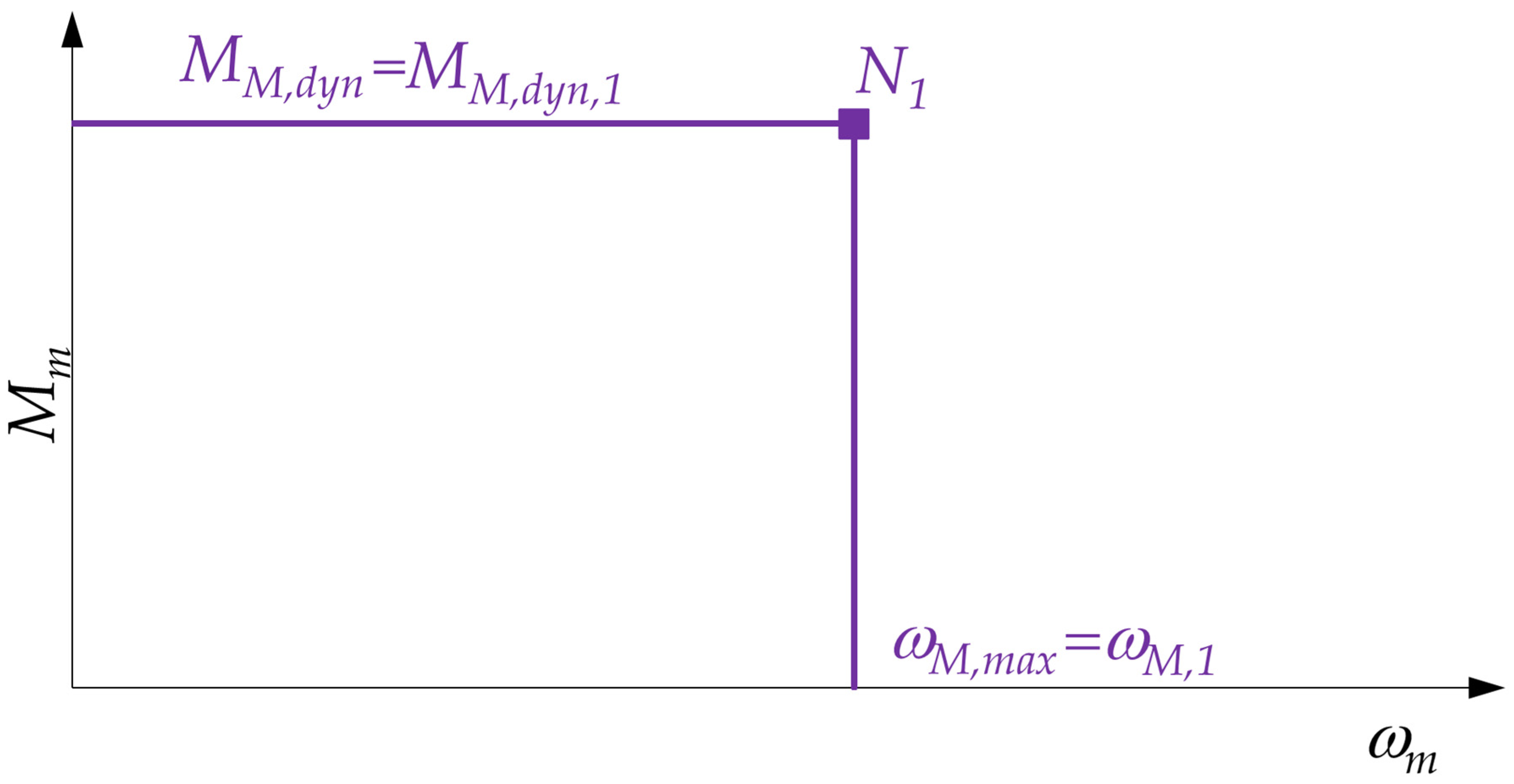
In this paper, the drive system operating ranges are assumed to be symmetrical in the four quadrants. A simple dynamic operating range of the brushless motor is initially used, with a constant torque denoted by
MM,dyn (
Figure 3). This is a common assumption because the motor speed often does not exceed
ωM,1. However, later, for the drive systems in which the limit torque of the dynamic operating range does depend on the motor speed,
Section 6 will explain how to solve the issue for many of them, by means of a procedure similar to that applied when
is constant and also explains how to fix the problem for the remaining drive systems, by means of a more complex method.
The specification of the load reference task allows the designer to know the joint angular speed and acceleration as functions of time, together with the load torque . In general, a numerical simulation, in which the motor and transmission sought are not included, provides these quantities.
3. The Method of Starting from a Given Transmission
Although the authors also appreciate other approaches, they observe that starting from a given transmission allows the designer to take into account all its functional and constraint parameters from the outset, which avoids any further check. In addition, assuming that the motor perfectly performs the reference task, it is possible to directly discard the gearboxes that do not allow it to be done. In general, with this approach, it is not possible to represent the parameters of the gearboxes as continuous functions of their design variables in order to proceed with an optimization.
Incidentally, it is easy to introduce among the various real transmissions a fictitious one that corresponds to the direct coupling between motor and load. It is also simple to consider an equivalent transmission that is made up of two real transmissions in series.
Once a transmission is taken into consideration, many ways of proceeding open to the designer. For the sake of simplicity, in this section this paper continues as in [
25] and finds the motors (with a rectangular dynamic operating range and in which the iron losses are negligible) that can be coupled with the given transmission, taken from a catalog, in order to perform the reference task from the point of view of the torque peak of the motor.
3.1. Admissible Transmissions
A candidate transmission is now taken into consideration, and therefore, all its parameters are known. As already explained in [
25], the first step is to find the transmission torque on load side and then to check if its torque and speed limits allow the reducer to move the load during the reference task, i.e., if it is admissible.
Denoting by
the moment of inertia of the transmission on load side, the transmission torque
on load side is a known function of time given by
The maximum value
of the transmission speed on load side is
or is a specification higher than the value given by Equation (2).
Obviously, the transmission speed on motor side, that is the motor speed
, is given by
The maximum absolute value
of
is given by
while the maximum absolute value
of the motor speed
is given by
Therefore, in order to be admissible, the speed reducer must meet the following set of inequalities:
If the given transmission is not admissible, it is discarded and a new speed reducer must be taken into account; otherwise, each of the candidate drive systems must be examined in order to check if it can be coupled with the given transmission to execute the reference task (from the point of view of the torque peak of the motor).
3.2. Admissible Drive System—Transmission Couples
Therefore, for an admissible transmission, a candidate drive system is now taken into consideration; it is characterized by its moment of inertia JM, maximum speed ωM,max and limit torque MM,dyn of its dynamic operating range. The torque peak of the motor must now be found. To this aim, it is necessary to introduce the following considerations involving the transmission parameters.
As explained in [
21,
22], the power flow through the transmission is direct if
and in this case, the direct efficiency
must be used, whereas the power flow is inverse if
and then, the inverse efficiency
must be considered.
Both efficiencies,
and
, can depend on the motor speed, and therefore also on the load speed, and on the load torque:
The effect of the transmission efficiencies is that, for the determination of the motor torque, instead of
, a different torque
must be considered on the load side of the transmission. If inequality (7) is met, it is given by
and in this case, it is amplified with respect to
; else, if inequality (8) is met, it is given by
and it is reduced with respect to
. For a given transmission
is a known function of time.
Denoting by
the moment of inertia of the transmission on motor side, the equilibrium equation of the system is expressed by
As in [
25], it is now convenient to define the torque
that also includes the known effect of the transmission inertia on motor side:
Moreover, is a known function of time.
At last, the motor torque is equal to
It is noteworthy that , and are known because they only depend on the specifications and the given transmission. Consequently, on the right-hand side only JM changes with the considered drive system.
The torque peak
Mm,max of the motor can now be found. In fact, the absolute value of the motor torque is given by
and
Mm,max is equal to
Therefore, a drive system can be coupled with the given transmission if it meets the following set of inequalities:
Since
JM and
MM,dyn are known for the motor into consideration, the calculation of its torque peak and the comparison with
MM,dyn are simple, and thus, the first inequality is easily checked. The second inequality is immediately checked too.
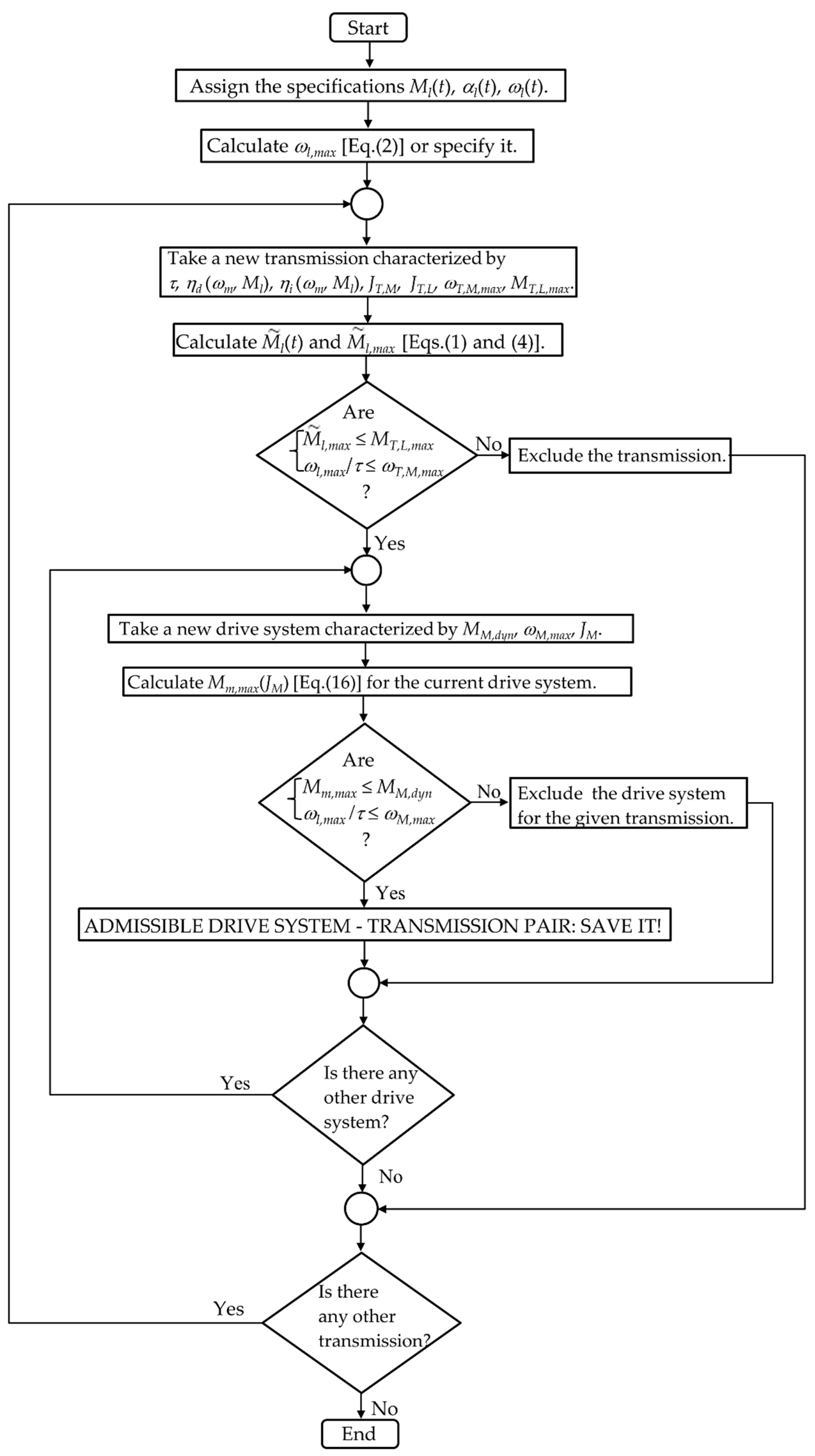
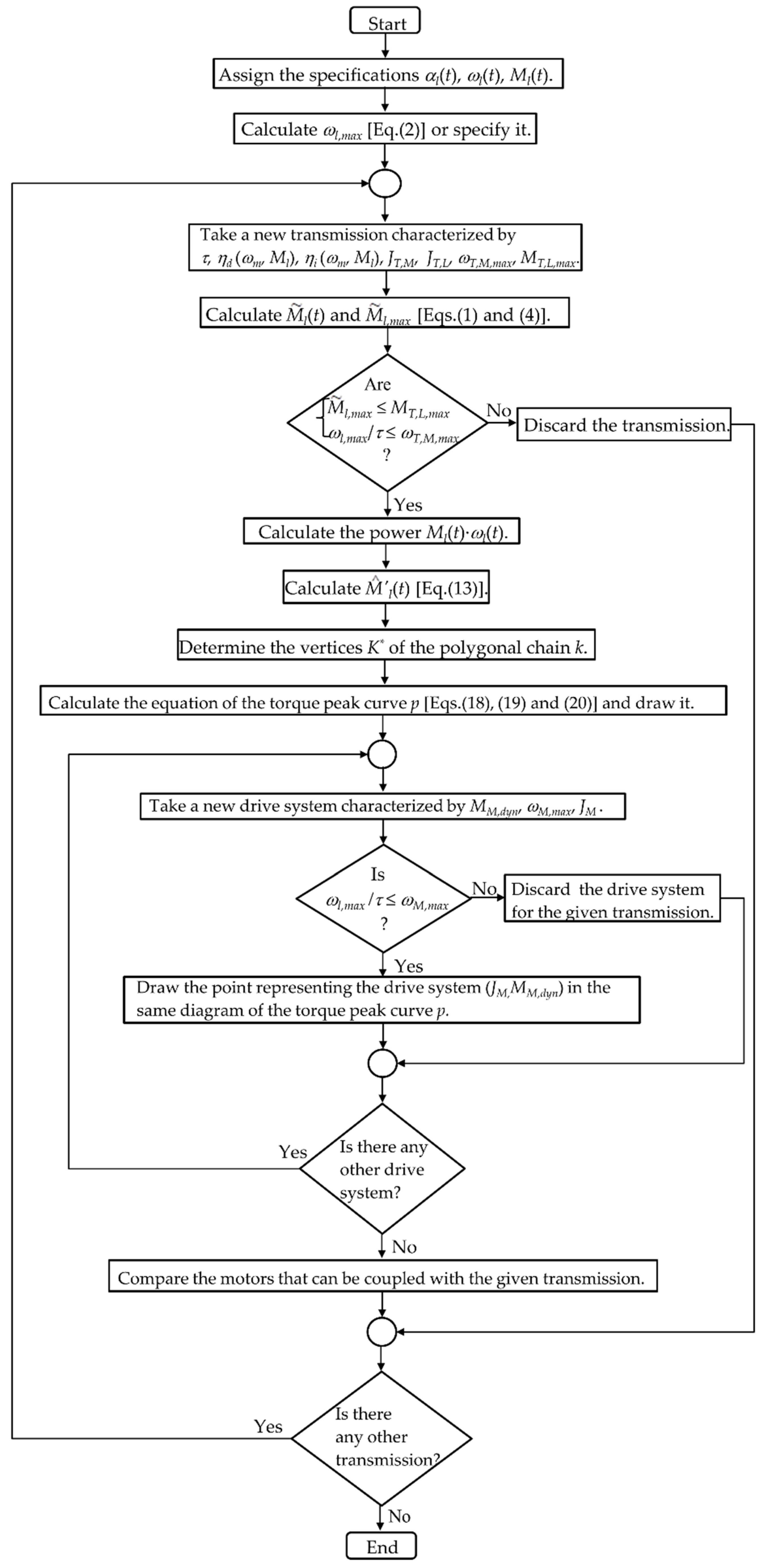
Figure 4 shows the flowchart of the whole procedure.
In this way, it is then possible to consider a feasibility matrix G whose generic element gr,s refers to the r-th transmission and the s-th drive system. If gr,s is equal to one, the s-th motor can be matched with the r-th transmission to carry out reference task of the load from the point of view of the torque peak of the motor; conversely, if it is equal to zero, the s-th motor and the r-th transmission, coupled together, cannot execute the reference task. Hence, this matrix concisely represents the result of the feasibility analysis from the perspective of the torque peak of the motor.
The motor thermal problem and the torque peak problem must be tackled together, by applying in parallel the two methods proposed in [
25] and in this paper. The definitive set of admissible drive system-transmission pairs is the intersection between the two sets, separately found. Since a matrix
F, similar to
G, was filled in [
25] for the motor thermal problem, it is clear that a logical AND between the two matrices provides a new matrix that shows all the drive system-transmission couples able to execute the reference task from both the points of view.
It is clear that some of the admissible drive system-transmission couples can be discarded due to other constraints that need to be respected. Sometimes this exclusion can be done from the beginning. For instance, when the overall weight of electronic drive, motor and transmission must not exceed a given threshold.
Although the subsequent optimization phase is beyond the scope of this paper and dealt with in its entirety is a complex problem, it is possible to make some considerations in the hypothesis of finding among the admissible drive system-transmission pairs, whose number is discrete, the one that minimizes a given objective function.
Some optimizations can be done maintaining the assumption that the motor perfectly performs the reference task. Some examples are the minimization of the overall cost of electronic drive, motor and transmission, their overall weight or, somehow, the volume of motor and transmission. Another example is the minimization of the energy dissipated in a cycle, taking also into account the power waste in the transmission, by assuming that inside the motor there is linearity between torque and current and that the power waste is only due to the Joule effect. It is of course possible to resort to a multi-objective optimization by means of a suitable linear combination of single-objective functions.
Other optimizations, such as those concerning the control performance, are more demanding, because they require at least the coupling of a complex model of the motor and the transmission, and also of the controllers, with a model of the rest of the machine.
4. Graphical Solution: Torque Peak Curve
Instead of an automated procedure, the designer often desires to resort to a graphical representation, which allows him a concise comparison among different solutions. In this case, it is convenient to fix a given transmission and to use a diagram in which the corresponding torque peak curve is drawn together with the motor representative points, as explained below.
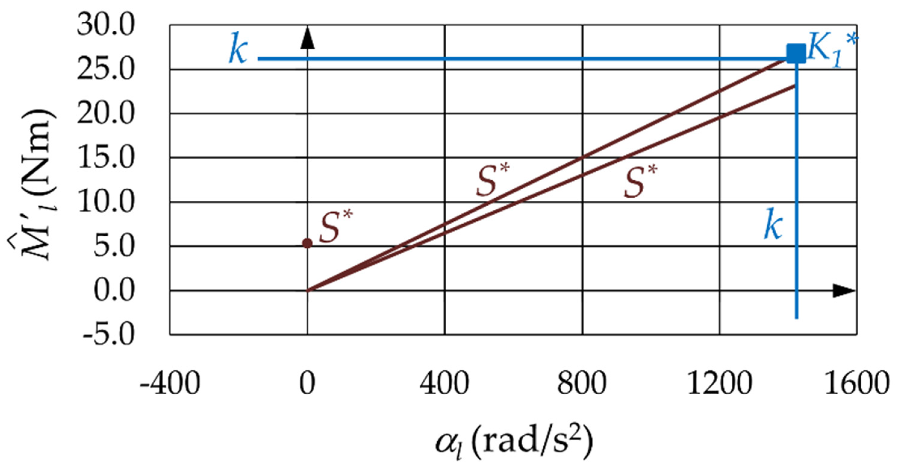
According to Equation (16), for each value of , the maximum value Mm,max assumed by over time must be found. The curve thus obtained is called torque peak curve and is denoted by p. The torque peak curve p lies in the first quadrant of the plane and can be drawn directly by means of Equation (16), in which is a parameter that increases from zero to a suitable maximum value. Here another way is proposed that allows the designer to find its analytical expression and to explain its shape. As will be explained later, it is continuous, consists of a sequence of segments and shows only one minimum point.
4.1. From Points to Points
In order to draw the torque peak curve
p, some of the conclusions explained in [
21] are reported here.
At a given time instant t, in the plane, Equation (15) corresponds to a curve lying in the first quadrant. This curve depends on the pair, which changes as time increases.
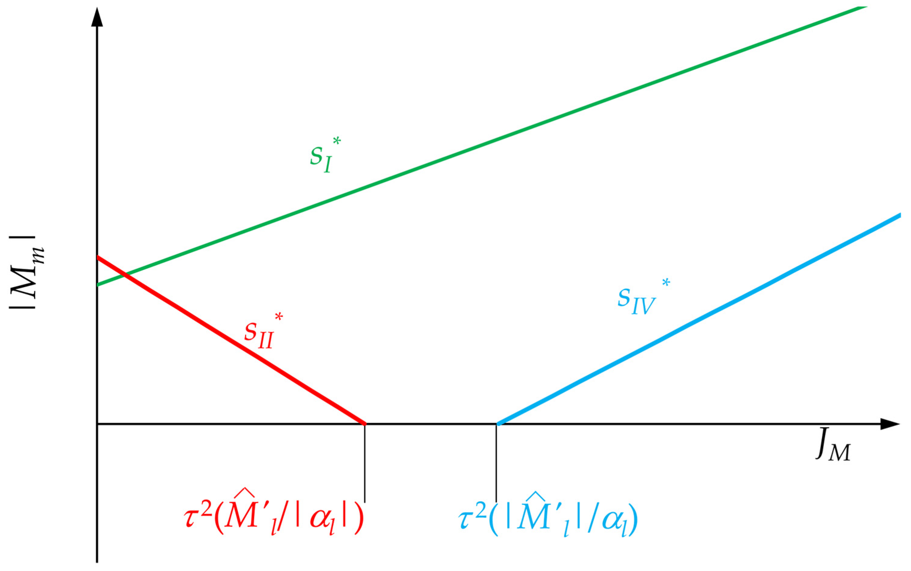
In the plane instead of considering the original points as time t varies, it is convenient to refer to a new set of points that derive from the original ones according with the following rules:
- −
If
and
have the same sign, positive or negative, or are both null, one set of points
lying in the first quadrant of the
plane must be taken into consideration; they have abscissa equal to
and ordinate equal to
. In the
plane the corresponding half-line
lies in the first quadrant (
Figure 5) and contributes to the ascending branch of the torque peak curve.
- −
If and have opposite sign, then two sets of points, symmetrical with respect to the origin, must be taken into account:
- (1)
The first set lies in the second quadrant of the
plane; these points have abscissa equal to
and ordinate equal to
. In the
plane the corresponding segment
lies in the first quadrant (
Figure 5) and can only contribute to the descending branch of the torque peak curve.
- (2)
The second set lies in the fourth quadrant of the
plane; these points have abscissa equal to
and ordinate equal to
. In the
plane the corresponding segment
lies in the first quadrant (
Figure 5) and can only contribute to the ascending branch of the torque peak curve.
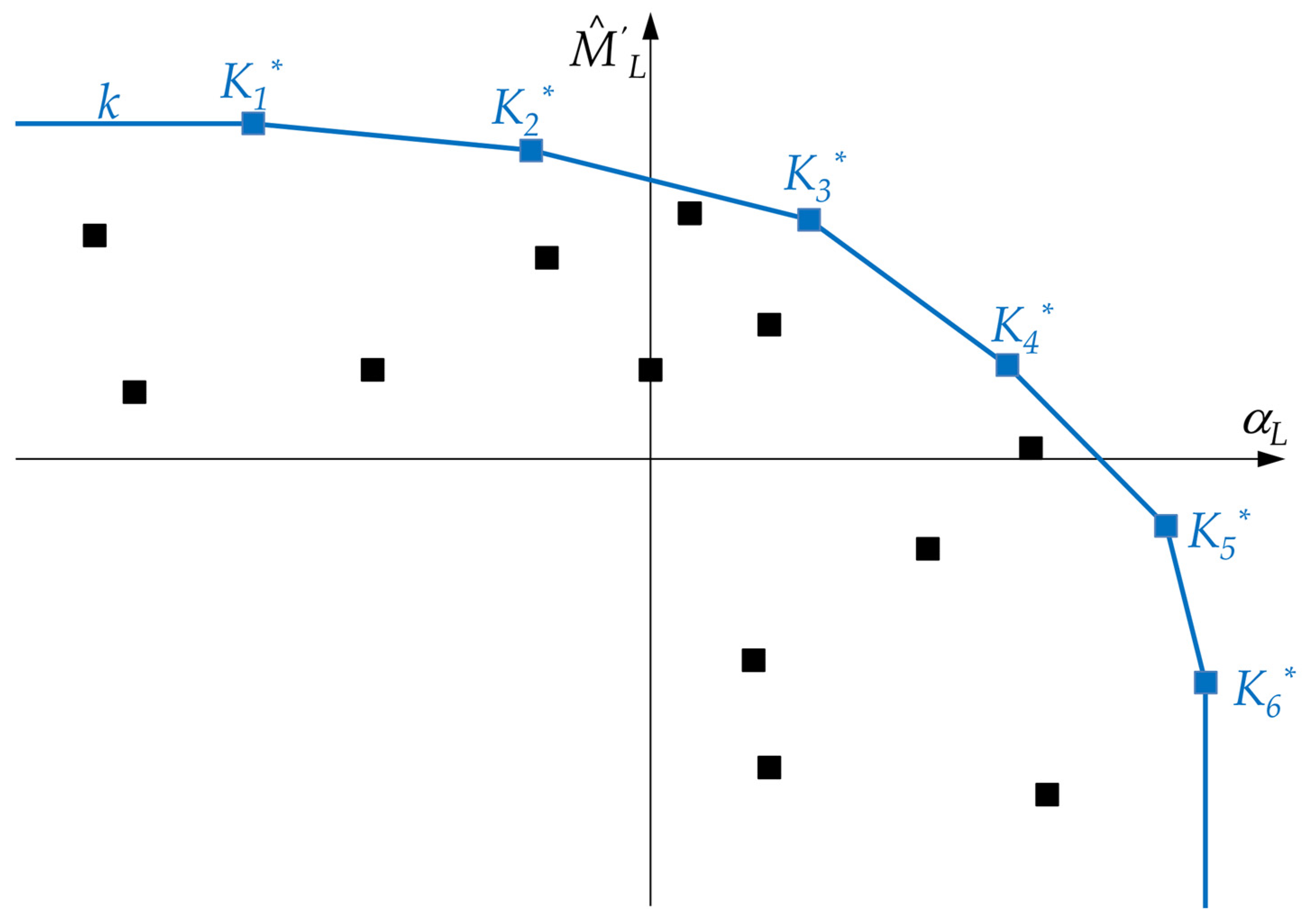
4.2. Points That Contribute to the Torque Peak Curve
Nevertheless, not all the points
S* lying in the first, second and fourth quadrant of the
plane contribute to the torque peak curve
p. Only few points affect this curve. Indicating their number with
n, they are denoted by
, with
j = 1, 2, …,
n. They are the vertices of a simple polygonal chain (
Figure 6), denoted by
k, with the following features:
- −
The concavity of k is always directed towards the same region of the plane, i.e., downwards and leftwards.
- −
All the other points S*, distinct from the vertices , lie inside this region.
- −
The first side of k is a horizontal half-line, the last side is a vertical half-line.
All the vertices affecting the torque peak curve p can be found by means of a simple software program.
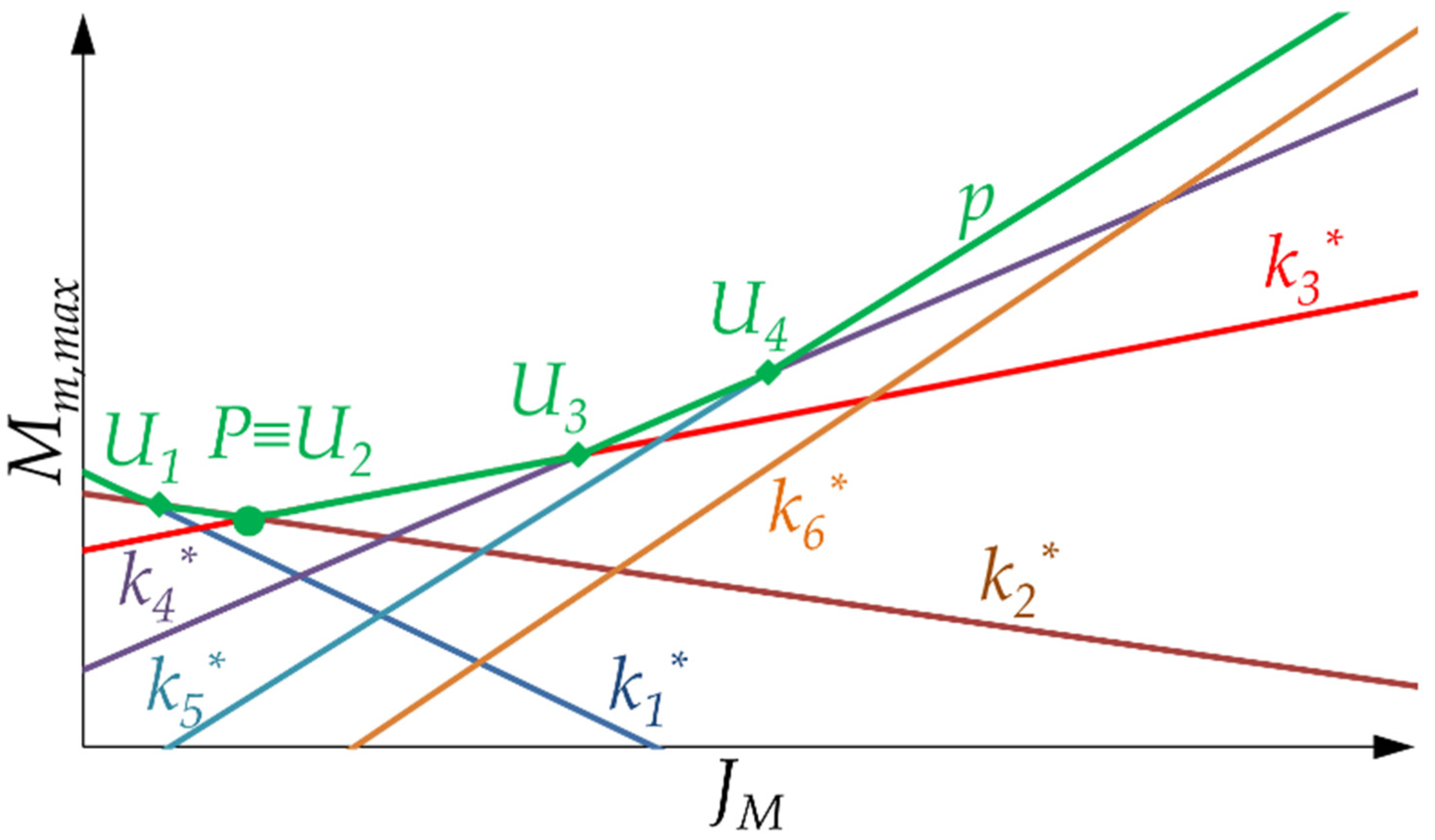
4.3. Shape of the Torque Peak Curve
It is now possible to find the equation of the torque peak curve. In the
JM-
Mm,max plane,
Figure 7 shows the different straight-lines
kj* corresponding to the points
shown in
Figure 6, and the resulting torque peak curve
p. The equation of the generic segment corresponding to the vertex
is
The abscissa of the intersection
Uj with the next branch is
while its ordinate is
Equations (18)–(20), whose parameters only depend on the reference task and the given transmission, allow the automatic writing of the equation of the global torque peak curve p.
This is a simple polygonal chain in the first quadrant of the JM -Mm,max plane. It is made up of consecutive segments, corresponding to the consecutive points . Only its last element is a half-line. These segments belong to straight lines having the following features:
- (1)
Their slope is negative or positive according to the sign of , i.e., according to the position of vertex either in the second quadrant of the plane or in the first and fourth.
- (2)
Their intersection with the ordinate axis is positive or negative according to the sign of , i.e., according to the position of vertex either in the first and second quadrants of the plane or in the fourth.
- (3)
Going from one point to the next one, the segment slope increases.
The first segment of the torque peak curve p can have either negative or positive slope; the last segment always has a positive slope. Therefore, generally, the torque peak curve is made up of a sequence of descending segments followed by a sequence of ascending segments: between the two sequences, there is a minimum point P. Obviously, if there is only a sequence of ascending segments, the abscissa of the minimum point P is null.
4.4. Drive System Representative Points
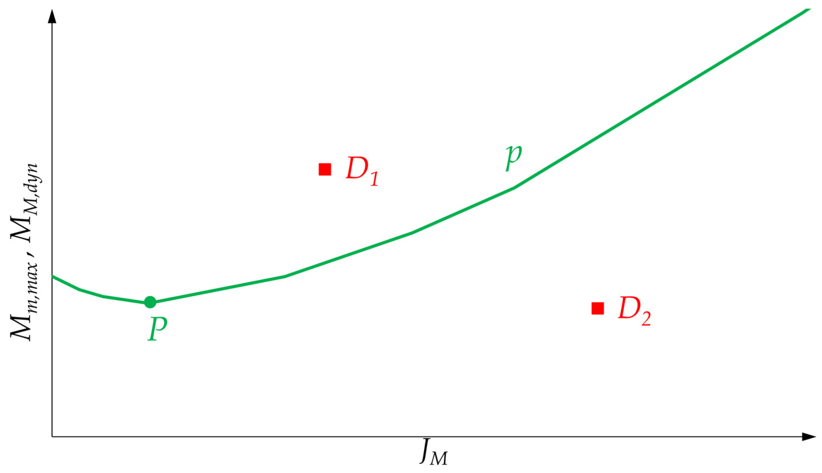
In the same diagram where the torque peak curve
p is plotted, each of the drive systems is represented by a point: the generic
j-th drive system corresponds to a point
Dj (
Figure 8) whose ordinate is its limit torque
MM,dyn and whose abscissa is the moment of inertia
JM of the motor.
Considering the first of inequalities (17), there are two cases:
- (1)
If the drive system representative point lies above the torque peak curve p, for example D1, the motor, coupled with the given speed reducer, is able to drive the load according to the reference task and is admissible.
- (2)
Conversely, drive systems whose representative points lie below curve p, for example D2, must be excluded for the given transmission.
In short, considering an admissible transmission and keeping in mind inequalities (17), a drive system can be coupled with this speed reducer from the point of view of its dynamic operating range if these simultaneous conditions are met:
- −
Its representative point does not lie below the torque peak curve
p in the diagram in
Figure 8.
- −
Its maximum achievable speed satisfies the second of inequalities (17).
Figure 9 shows the flowchart of the graphical procedure. Until the analysis of admissibility of the given transmission, it coincides with the flowchart in
Figure 4.
Both the torque peak curve and the rms torque curve in [
25] show a minimum point, even though in general the abscissas of these points are different. In trend line, drive systems whose representative points lie above these curves and near the minimum points are admissible for the given transmission and characterized by a smaller cost and size. However, also the cost and size of the transmission must be kept into account.
This procedure also allows the designer to identify on which elements of the specifications (and the transmission parameters) the shape of the torque peak curve depends. Sometimes, the specifications are not rigid, and the designer can slightly modify them in view of other benefits, for example, the choice of a motor otherwise to be discarded or, for an interesting admissible drive system–transmission couple, the decrease of the period of the reference task. However, the effects of these modifications must also be examined with reference to the thermal problem of the motor.
5. A Case Study
The same flying machine for sealing and cutting already examined in [
25] from the point of view of the motor thermal problem is here analyzed from the point of view of the torque peak of the motor. The reference task is periodic with a period of 0.08 s and is characterized by a global rotation of the load of 2π/3 rad. The acceleration and speed of the load together with the global torque
Ml can be found in [
25] as functions of time.
The same transmission considered in [
25] is now taken into account. Its characteristics are summarized in
Table 1. The direct and inverse efficiency do not depend on speed.
In [
25], this transmission was already found admissible.
The same four drive systems
D1,
D2,
D3 and
D4 considered in [
25] are candidate to move the load. Their dynamic operating range is rectangular, and their characteristic parameters are shown in
Table 2. As already shown in [
25], all the four motors meet the speed inequality (17).
During the period, the power flow through the transmission shows an alternation from motor to load (when is positive) and from load to motor (when is negative).
To draw the torque peak curve
p requires the determination of the vertices
in the
plane. In
Figure 10, the brown curves are the locus of a point
S*. The polygonal chain
k is made up of a horizontal and a vertical half-line, and only vertex
gives contribution to the torque peak curve
p.
In
Figure 11, the representative points
D1,
D2,
D3 and
D4 of the four drive systems taken into consideration are drawn, together with the torque peak curve
p. Since points
D2,
D3 and
D4 lie above curve
p, only these motors can be coupled with the given transmission from the point of view of the limit torque
MM,dyn of the dynamic operating range.
Since only drive systems
D3 and
D4 gave a positive result from the point of view of the motor thermal problem [
25], finally, these are the only motors that, coupled with the given transmission, are able to perform the reference task from all the points of view.
7. Effect of a Viscous Torque inside the Motor
This section shows how the proposed procedure can be modified when inside the motor, there is a considerable viscous torque due to the iron losses. The treatment is similar when, instead of a viscous torque, there are other resistant torques that are known functions of speed. The equations are those of a DC motor. Linearity is assumed between the ideal torque
of the motor and current
i, according to the torque constant
:
Taking into account the iron losses, the available torque
to accelerate the motor itself and to move transmission and load is given by
where
, because of the equilibrium equation, is given by Equation (14).
The motor current assumes the value:
Both the thermal problem of the motor and the torque peak problem of the drive system will now be analyzed.
7.1. Thermal Problem of the Motor
From the point of view of the power losses inside the motor, there are now two differences:
- (1)
As i changes, the Joule losses in the winding resistances change too.
- (2)
The iron losses are added to the copper losses.
The dissipated power is given by
where
R denotes an appropriate resistance of the windings, and the second term refers to the effect of the viscous torque (iron losses).
According to Equation (23), the dissipated power assumes the value
If the thermal behavior of the motor is governed by a first order differential equation and the periodic reference task has a period
T much lesser than the thermal time constant of the motor, in this differential equation on the right-hand side, there is a constant known term that is the average dissipated power in the period. This is due to the fact that the variations of the dissipated power in the period are filtered with respect to the average value, denoted by
, which, according to Equation (25), is given by
Keeping in mind Equation (14), in the last term, the integral can be written as
The first term on the right-hand side is equal to zero because at the end of the period the speed assumes its initial value. The second term can be calculated and is denoted by .
Hence, the dissipated power assumes the expression
If
is the stall torque, in mechanical and thermal steady state conditions, at the limit temperature that the motor can reach, the corresponding dissipated power at the different speeds is always given by
The subscript S1 is due to the fact that this is the dissipated power along the limit curve of the continuous duty operating range S1.
In order to avoid the over-heating of the motor, the average dissipated power in the period must be lesser than this value:
The result is
and after dividing all terms by
,
Isolating
on the left-hand side, the following inequality is obtained
According to [
25],
is a known function of
, called rms torque curve
r, given by
with
The same procedure shown in [
25] can now be used, with the same rms torque curve
r, which is a hyperbola in the first quadrant of the
plane that does not depend on the drive system (
Figure 13). Nevertheless, the representation of the motor is different. In fact, according to Equation (32), an
equivalent motor is represented by a point whose abscissa is still its moment of inertia
, whereas its ordinate is now the equivalent torque
given by
which depends not only on the motor but also on the transmission and the reference task.
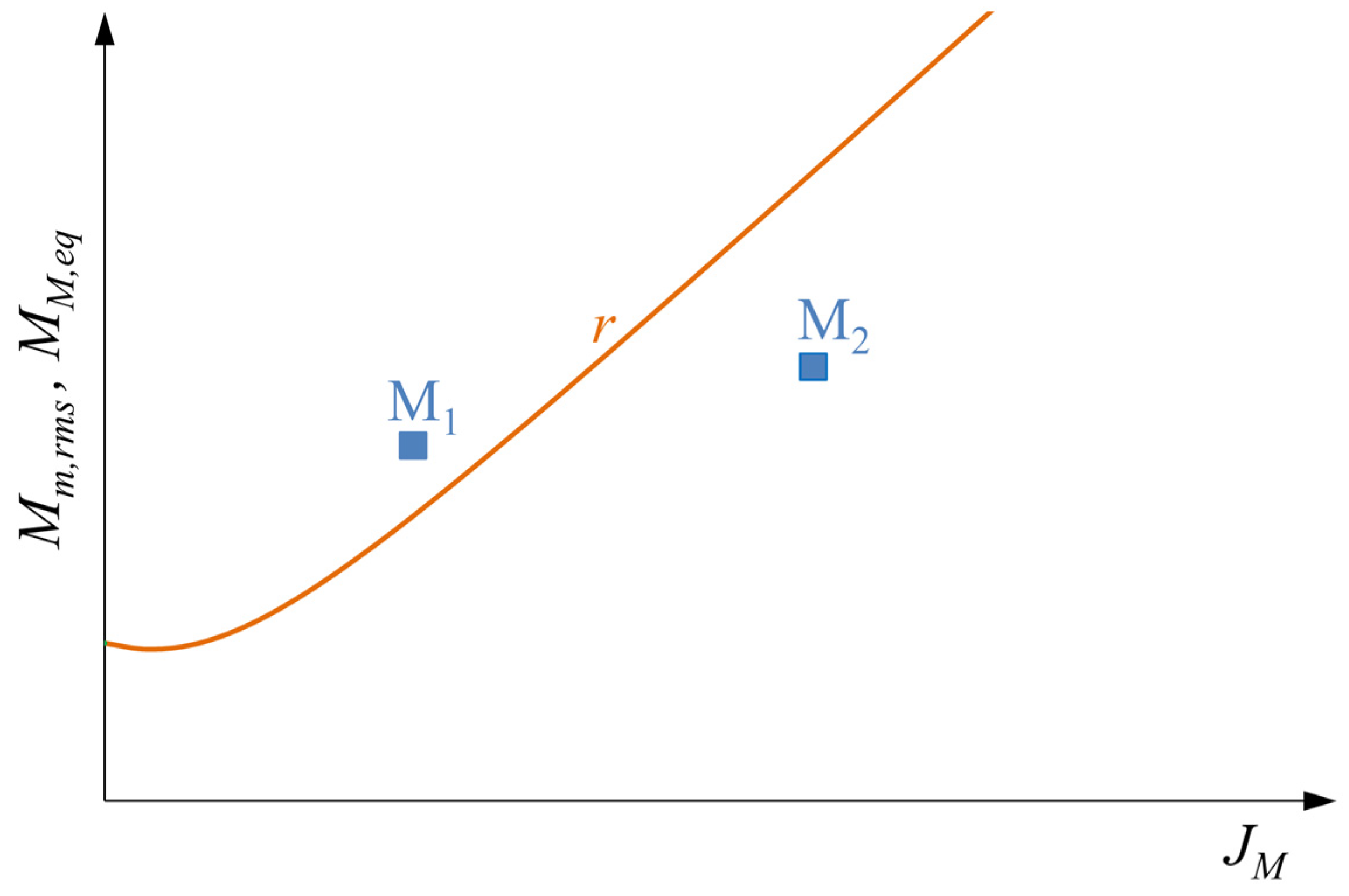
If the representative point of the equivalent motor lies above the rms torque curve r (motor M1), the drive system can be coupled with the given transmission in order to perform the reference task (from the point of view of the thermal problem of the motor). On the contrary, if it lies below (motor M2), it must be definitively excluded.
If, instead of a graphical representation, the designer decides to use an automated procedure, Equations (33) and (34) allow him to do it easily.
7.2. Torque Peak Problem of the Drive System
As regards the torque peak problem, the available motor torque is given by Equation (22), but the limit torque
of the dynamic range corresponds to the ideal motor torque
given by Equation (21) when the current reaches the maximum value
allowed by the electronic driver:
According to Equation (22), the ideal torque of the motor is equal to
In order to avoid the torque peak problem, the following inequality must be respected
Keeping in mind Equation (14), the result is
This inequality is like the first of inequalities (17), by replacing the torque
given by
instead of
in the expression of
:
The difference with respect to the first of inequalities (17) is that the right-hand side also depends on the motor, through the parameter b.
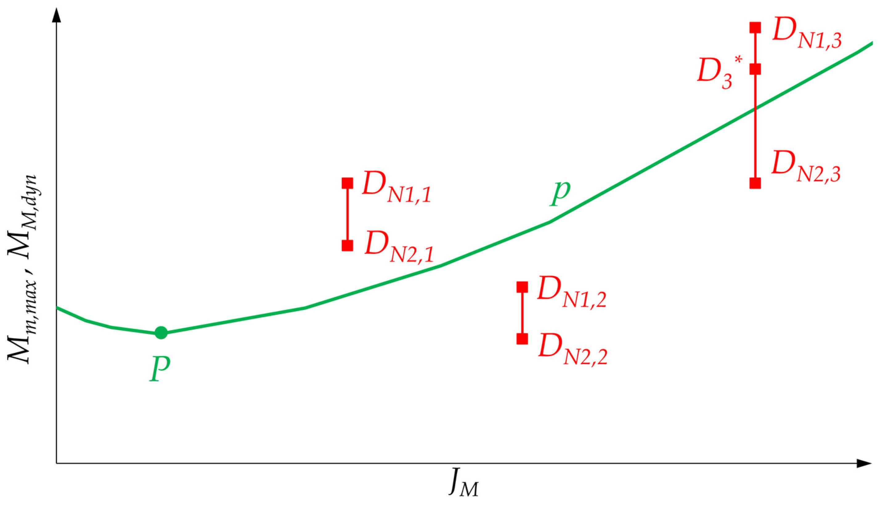
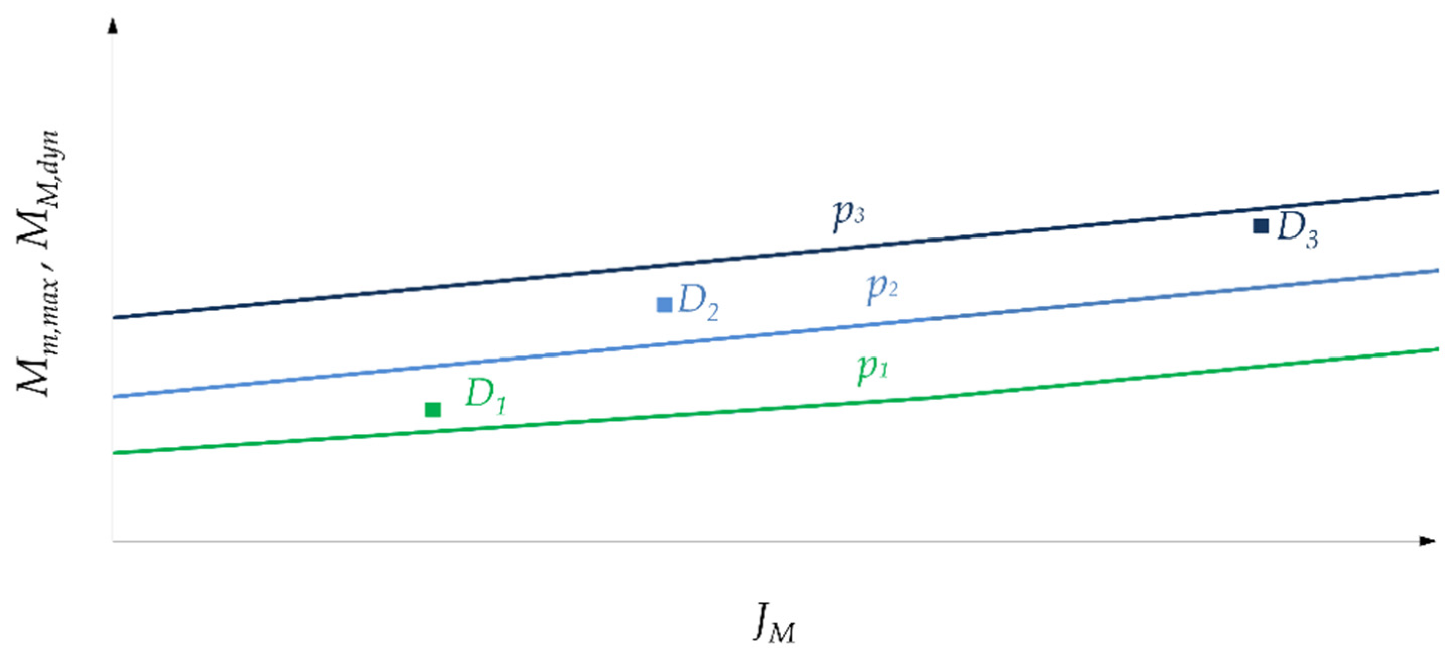
Hence, the corresponding torque peak curve
p now depends not only on the reference task and the transmission but also on the motor. Nevertheless, it obviously has the same general characteristics of a torque peak curve, already seen in
Section 4. In particular, this curve shows a possible descending branch, a minimum point and an ascending branch. Obviously, by changing
b as a parameter, the corresponding curves are different, for example, as regards the position of the minimum point (
Figure 14).
Hence, in the first quadrant of the plane
, a family of curves, with
b as a parameter, can be drawn. On the contrary, each drive system is still represented by the same point as in
Section 4, whose abscissa is its moment of inertia
and ordinate is
Nevertheless, this point must be labeled by means of the corresponding value of
b, in order to compare it with the corresponding torque peak curve.
If the representative point of the drive system lies above the corresponding curve (drive systems D1 and D2), this drive system can be coupled with the given transmission in order to perform the reference task (from the point of view of the torque peak problem). Otherwise (drive system D3), it must be definitively excluded.
If instead the designer decides to proceed with an automated calculation, Equations (42) and (17) permit him to do it easily.
8. Conclusions
This work deals with the admissible drive system-transmission couples from the point of view of the torque peak of the motor, i.e., those couples that are able to perform the reference task from this perspective. It proposes a method by which all these couples are found from the outset. This means that transmission ratio, reducer efficiencies and their dependency on speed and torque, inertia of the speed reducer, limits of speed and torque of the reducer, motor inertia, limits of speed and torque of the drive system, i.e., all the elements playing a role in the choice, are taken into account in a complete and effective way. Furthermore, the most general case, in which during the cycle there is alternation between direct and inverse power flow through the transmission, is considered. This method allows the designer to avoid any further check.
Starting from the common case of a rectangular dynamic operating range of the drive system, the rationale of the proposed method is to take the candidate transmissions from the catalogs one by one, so that all their parameters are known from the outset.
After excluding the not admissible transmissions, whose limits of speed and torque are not compatible with the reference task, for each of the other reducers, all candidate drive-systems are examined one at a time. For each motor, its torque peak during the reference task is determined by means of an equation that takes into account all the most significant factors on which it depends. Its comparison with the limit torque of the dynamic operating range allows an automatic check to ascertain if the drive system under analysis can be coupled with the transmission taken into consideration.
In addition to an automated procedure, a graphical representation provides the designer a concise view of all the drive systems that can be coupled with a given admissible transmission. More in detail, a torque peak curve can be drawn as a function of the unknown moment of inertia of the motor; this curve is only related to the reference task and to the transmission parameters. In this diagram, each drive system is represented by a point that is compared with the torque peak curve in order to accept or exclude the motor. This graphical interpretation must be repeated for each admissible transmission.
Furthermore, for many drive systems whose dynamic operating range is non-rectangular, this work explains how to apply a similar procedure. For the remaining drive systems, a more complex method is explained.
Finally, the paper shows how the proposed method can be applied to motors that present an internal viscous torque due to the iron losses (also with reference to the thermal problem of the motor).
Therefore, this work, together with paper [
25], which similarly deals with the motor thermal problem, is an interesting instrument to determine from the outset the admissible drive system-transmission couples for a given reference task. An optimization phase must follow this feasibility stage.
In a future work, the authors will study the non-linearities of the motor that influence its choice.


