Article

Research on Vehicle Adaptive Cruise Control Method Based on Fuzzy Model Predictive Control

School of Mechanical and Precision Instrument Engineering, Xi’an University of Technology, Xi’an 710048, China
*
Author to whom correspondence should be addressed.
Machines 2021, 9(8), 160; https://doi.org/10.3390/machines9080160
Submission received: 16 June 2021 / Revised: 5 August 2021 / Accepted: 6 August 2021 / Published: 8 August 2021

Abstract

:
Under complex working conditions, vehicle adaptive cruise control (ACC) systems with fixed weight coefficients cannot guarantee good car following performance under all conditions. In order to improve the tracking and comfort of vehicles in different modes, a fuzzy model predictive control (Fuzzy-MPC) algorithm is proposed. Based on the comprehensive consideration of safety, comfort, fuel economy and vehicle limitations, the objective function and constraints are designed. A relaxation factor vector is introduced to soften the hard constraint boundary in order to solve this problem, for which there was previously no feasible solution. In order to maintain driving stability under complex conditions, a multi-objective optimization method, which can update the weight coefficient online, is proposed. In the numerical simulation, the values of velocity, relative distance, acceleration and acceleration change rate under different conditions are compared, and the results show that the proposed algorithm has better tracking and stability than the traditional algorithm. The effectiveness and reliability of the Fuzzy-MPC algorithm are verified by co-simulation with the designed PID lower layer control algorithm with front feedforward and feedback.

1. Introduction

Advanced Driver Assistant Systems (ADAS) [1] are currently widely deployed in automobiles. Among them, the adaptive cruise control (ACC) system is one of the most popular ADAS. The control method of the ACC system generally adopts layered control [2].
The upper-level control algorithm calculates the expected longitudinal acceleration of the vehicle based on the current state of the vehicle’s motion, which is becoming more and more diversified. Zhang et al. [3] analyzed a PID-type vehicle-following controller for different spacing policies and designed a new vehicle-following controller. Chan et al. [4] used a distributed arithmetic structure based on FPGA-based high-efficiency PID as the ACC control algorithm. The study of Cananle et al. [5] personalized an adaptive cruise control with stop and go features (ACC/S&G) for urban scenery. Daniele et al. [6] adopted an adaptive method involving the terminal cost and constraint set MPC approach, which is commonly used for fixed set-point regulation, in order to achieve good tracking of a time-varying reference trajectory. Naus et al. [7] selected followability, driving comfort and fuel economy as the system optimization goals in the multi-objective ACC system designed based on MPC, so that the vehicle can improve the fuel economy on the premise of safe following and driving comfort. Firoozi et al. [8] designed an ACC system based on MPC considering the motion of the front vehicle and road gradient. Tran et al. [9] proposed an ACC system design method combining an analytical method and a stochastic MPC method. Eom et al. [10] proposed a new human–computer interaction design method, in which the proposed standards were used to determine the compatibility of machine models and interface models. If the models were not compatible, one or both models were modified to make them compatible. The results show that the modified machine model provides a more compact, acceptable, efficient and secure interface than the modified interface model. Subiantoro et al. [11] used a multi-level linear model to describe the nonlinear behavior of the ACC system, but the relationship between the parameter model matrices remained linear. A multi-stage predictive control based on nonlinear model predictive control (NMPC) was designed. Liu et al. [12] proposed an economical ACC to improve the fuel economy of hybrid electric vehicles (HEV) by simultaneously optimizing vehicle route, velocity, and power system control. Motivated by connected and automated vehicle (CAV) technologies, Zhao et al. [13] proposed a data-driven optimization-based MPC modeling framework for the Cooperative Adaptive Cruise Control (CACC) of a string of CAVs under uncertain traffic conditions. Wu et al. [14] designed an ACC system based on an active braking algorithm to improve vehicle safety and comfort. Jiang et al. [15] considered the driver’s risk sensitivity under system and measurement uncertainty, and proposed a personalized stochastic optimal adaptive cruise control algorithm. It can be seen that the research on upper control algorithms is increasingly focused on how to better coordinate multiple objectives to meet real needs.
The lower controller is the actuator of the ACC system. Taking the expected acceleration output from the upper controller as input, the actual acceleration of the vehicle remains consistent with the expected acceleration output of the upper controller by controlling the accelerator pedal and brake pedal, so as to achieve the purpose of following the front vehicle. Satoru et al. [16] designed the lower controller of the ACC system based on PID control. It can keep the actual acceleration of the ACC system vehicle consistent with the expected acceleration output through the upper controller of the ACC system. Yi et al. [17] designed the lower controller of the ACC system based on PI control and feedforward control theory, which improved the response speed of the system. Fancher et al. [18] established an inverse longitudinal dynamic model and introduced a compensation algorithm to improve the model’s anti-interference performance. To make the lower controller faster and achieve a more accurate control response and real-time performance, Li et al. [19] designed acceleration and braking look-up tables based on test data, and formulated acceleration and braking conversion rules. Zhang et al. [20] designed a lower controller suitable for electric vehicles, which enables energy to be recovered during the braking process to improve energy economy. Cheng et al. [21] designed a lower controller. The brake pressure calculation module used a slip ratio controller, and the electronic throttle opening calculation module used a look-up table method. David et al. [22] used a neural network to design a deceleration prediction system for an adaptive cruise control unit. The neural network was used to refine the determination of deceleration value of the vehicle in front of static or dynamic obstacles, and at the same time, some influences affecting the braking process are included, so as to improve the driving safety. Therefore, the lower controller tends to be more and more simplified while meeting the requirements.
In the process of following, we need to constantly change the weight of following according to different following environments to better coordinate multiple goals. At present, most of the current research algorithms cannot take into account multiple goals, and it is difficult to adapt to the changing following environment. In this paper, the longitudinal kinematics model between the two vehicles is established, and the objective function and constraint conditions are designed considering the vehicle speed, acceleration, acceleration rate of change, distance error and relative speed. A relaxation factor is introduced to soften the hard constraint boundary and expand the feasible region. Under the MPC theory, fuzzy rules of relative distance error, relative speed and vehicle following weight coefficient are designed. The variable weight coefficient method based on fuzzy control updates the data online in real time to adapt to the complex traffic conditions, and the simulation experiments are compared in the MATLAB environment. The lower controller adopts a threshold-based switching strategy, uses PID feedback control to minimize the acceleration error, and designs a braking force controller and a throttle opening controller. Finally, the algorithm is verified.

2. Fuzzy-MPC Based Vehicle Multi-Target Upper Controller

An upper control algorithm for ACC systems, based on fuzzy model predictive control (Fuzzy-MPC) theory, is designed in this paper. The four control objectives of followability, safety, comfort, and fuel economy are used as references for the design of performance indicators and system constraints, and the optimization objective is transformed into a constrained quadratic programming problem to be solved. At the same time, in order to meet the driving requirements of vehicles in different driving environments, a variable weight coefficient method is proposed based on fuzzy control.

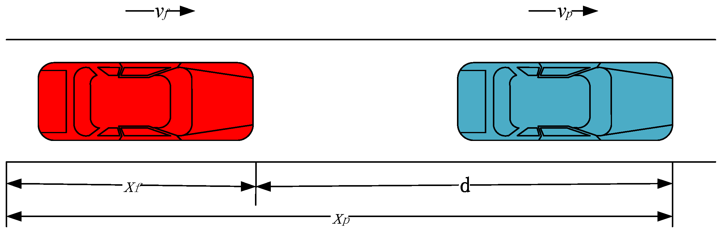
2.1. Longitudinal Kinematics Modelling of Two Vehicles

During the car following process, the ACC system maintains a safe distance between the two vehicles and can keep up with the target vehicle smoothly and quickly. The longitudinal kinematics relationship between the two vehicles is shown in Figure 1.
According to the longitudinal kinematics relationship and spacing strategy between the ACC vehicle and the target vehicle [23], x ( k ) = [ d , v f , v r e f , j ] T is selected as the state variable of the ACC system. The longitudinal kinematics state equation of ACC vehicle is expressed as Equation (1).
x ( k + 1 k ) = A x ( k ) + B u ( k ) + G φ ( k )
where x ( k + 1 k ) is the predicted value of k + 1 at time k, u ( k ) is the control variable at time k , and φ ( k ) is the target vehicle acceleration disturbance at time k. The coefficient matrices A , B and G are, respectively, shown below.
A = [ 1 0 T s 1 2 T s 0 0 1 0 T s 0 0 0 1 T s 0 0 0 0 1 T s τ 0 0 0 0 1 τ 0 ] B = [ 0 0 0 T s τ 1 τ ] G = [ 1 2 T s 2 0 T s 0 0 ]
where T s is the sampling period and τ is the time delay constant of the lower controller.
Since safety, followability, comfort, and fuel economy are important indicators for evaluating ACC vehicles, let y ( k ) = [ Δ d , v r e f , a f , j ] T be the optimized performance index vector, Δ d the relative distance ( Δ d = d d s a f e ), d s a f e ( d s a f e = v t h + d 0 ) the expected safe spacing with time headway( t h ), and d0 the minimum safe spacing greater than the length of the vehicle.
y ( k ) = C x ( k ) S
where the coefficient matrices C and S are as follows.
C = [ 1 t h 0 0 0 0 0 1 0 0 0 0 0 1 0 0 0 0 0 1 ] S = [ d 0 0 0 0 ]
Due to differences in vehicle models and interference from the external environment, there will be a certain error between the predicted value of the prediction model and the actual value in the ACC system. In order to reduce this error, feedback correction is used to improve the accuracy and robustness of the ACC system. Therefore, according to the principle of feedback correction, the prediction error at time k is described as follows.
e ( k ) = x ( k ) x ( k | k 1 )
where e ( k ) is the prediction error, x ( k ) is the actual state of the system at time k , and x ( k | k 1 ) is the predicted value of k at time k 1 .
In order to improve the accuracy of the system’s future prediction values, the weighting matrix is used to adjust the prediction error. Thus, Equation (1) can be transformed into Equation (4).
x ( k + 1 k ) = A x ( k ) + b u ( k ) + G φ ( k ) + W e ( k )
where x ( k ) is the actual state variable at time k , u ( k ) is the control variable at time k , and W is the correction matrix ( W = d i a g ( w 1 , w 2 , w 3 , w 4 , w 5 ) , w i ( 0 , 1 ) ).
Considering the restrictions of safety, the vehicle itself and traffic laws, etc., relative distance, vehicle speed, acceleration, acceleration rate of change, and control variables are restricted within a certain range. In the process of MPC rolling optimization, for cases in which there is no solution under hard constraints, the method in [24] is used, which treats the constraints that need to be widened differently. Therefore, the constraints are relaxed.
{ d d 0 + ε 1 ξ max d v f min + ε 2 ξ min v f v ( k ) v f max + ε 2 ξ max v f a f min + ε 3 ξ min a f a ( k ) a fmax + ε 3 ξ max a f j e r k min + ε 4 ξ min j e r k j e r k ( k ) j e r k max + ε 4 ξ max j e r k u min + ε 5 ξ min u u ( k ) u max + ε 5 ξ max u
where ε i 0 ( i = 1 ~ 5 ) is the relaxation factor, ξ max d , ξ max v f , ξ max a f , ξ max j e r k , ξ max u ≥ 0 is the relaxation coefficient of the upper bound of the hard constraint, and ξ min v f ,  ξ min a f ,  ξ min j e r k , ξ min u ≥ 0 is the relaxation coefficient of the lower bound of the hard constraint.

2.2. Scrolling Optimization

Select safety, followability, driving comfort and fuel economy as the optimization performance indicators, and optimize the control variables and prediction errors, so that the ACC vehicle can better track the target vehicle. The final objective function is determined as follows.
J = i = 1 N P [ y p ( k + i | k ) y r e l ( k + i | k ) ] T Q [ y p ( k + i | k ) y r e l ( k + i | k ) ] + i = 1 N c u ( k + i ) T R u ( k + i )
where y p ( k + i | k ) is the performance index vector in the prediction time domain, ( k + i | k ) represents that k is the prediction of k + i time under the time, y r e l is the reference trajectory ( y p ( x ) ) , N p is the prediction time domain, N c is the control time domain, u is the control variable, R is the weight of u ( R = 1 ) and Q = ( ς d , ς v r e f , ς a f , ς j ) are weight coefficients.
Therefore, the objective function of the multi-objective ACC upper control algorithm will eventually be transformed into a constrained quadratic programming problem.
{ min U ˜ T H U ˜ + 2 f U ˜ s . t . A u U b u
where
U ˜ = [ U   ε ] T H = [ Γ R + F ρ T Γ Q F ρ 0 0 ρ ] f = [ x ( k ) T ( C p T C T Ψ ) Γ Q   Γ R + ϕ T S p T   Γ Q F ρ ( D p T D p T Ψ ) Γ Q F ρ + e ( k ) T L p T   Γ Q F ρ 0 ] A u = [ P B p P B p I I ξ ¯ max x ξ ¯ min x ξ ¯ max x ξ ¯ min x ] b u = [ N P G p ϕ P A p x ( k ) P W p e ( k ) R + P G p ϕ + P A p x ( k ) + P W p e ( k ) U max U min ] Γ Q = [ Q Q Q Q ] Γ R = [ R 0 0 R ] Ψ = [ Λ Λ N p ] ξ ¯ max x = [ ξ max x ξ max x ξ max x ] ξ ¯ min x = [ ξ min x ξ min x ξ min x ] ξ ¯ max = [ ξ max ξ max ξ max ] ξ ¯ min = [ ξ min ξ min ξ min ] P = [ p 0 0 p ] R = [ r r r ] N = [ n n n ] U max = [ u max u max u max ] U min = [ u min u min u min ] ξ min x = [ ξ min d 0 0 0 0 0 ξ min v f 0 0 0 0 0 ξ min a f 0 0 0 0 0 ξ min j e r k 0 ] ξ max x = [ ξ max d 0 0 0 0 0 ξ max v f 0 0 0 0 0 ξ max a f 0 0 0 0 0 ξ max j e r k 0 ] ξ min = [ 0 0 0 0 ξ min u ] ξ max = [ 0 0 0 0 ξ max u ] P = [ 1 0 0 0 0 0 1 0 0 0 0 0 0 1 0 0 0 0 0 1 ] r = [ d 0 v f min a f min j e r k min ] n = [ inf v f max a f max j e r k max ]
where I is the unit vector and the dimension is N c , and Λ is the reference trajectory coefficient.

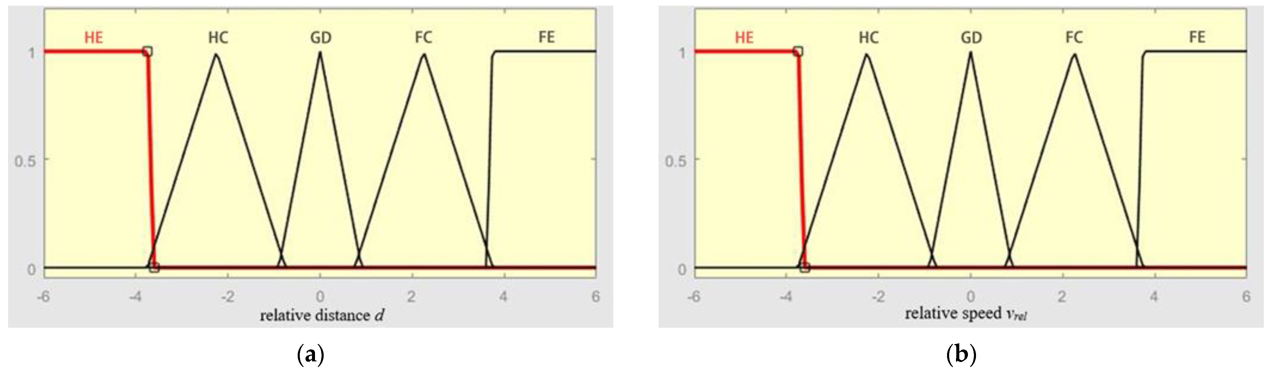
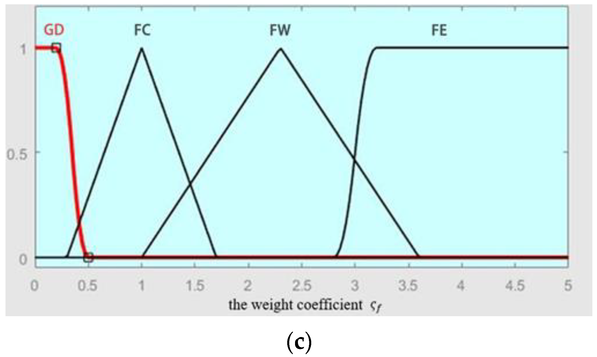
2.3. Variable Weight Coefficient Design Based on Fuzzy Control

In a complex and changeable traffic environment, different traffic conditions require different weighting factors. We design a variable weight coefficient based on fuzzy control theory to improve the adaptability of the ACC system and ensure that it can follow the target vehicle smoothly and safely.
The relative distance d, relative speed v r e l , and the weight coefficient of the vehicle following ς f ( ς f = ς d = ς v r e f ) are, respectively, blurred into 3 sets.
{ δ : v r e l : ς f [ H F H C G D F C F E ] [ H E H C G D F C F E ] [ G D F C F W F E ]
where HE, HW, HC, GD, FC, FW, FE represent negative large, negative medium, negative small, zero, positive small, positive medium, and positive large, respectively.
Set the fuzzification range of d to [−80, 80] m. When the value of d is near zero, it belongs to GD. v r e l is limited to [−20, 20] m/s. The comfort weight coefficient ς c ( ς c = ς a f = ς j ) is always set to 1. At the same time, the change area of ς f is set as [0, 5]. When ς is at [0, 1], it is believed that the demand for comfort and fuel economy is greater; and when ς is at [1, 5], it is indicated that the demand for vehicle following safety is greater. From this, the membership functions of the input variables and output variables can be obtained, as shown in Figure 2.
Considered comprehensively, the designed fuzzy control rules of c f , d and v r e f are shown in Table 1.

2.4. Numerical Simulation Verification

In order to verify the effectiveness of Fuzzy-MPC, the traditional MPC algorithm is compared in MATLAB and normal and emergency conditions are selected for simulation. The simulation parameters are shown in Table 2.

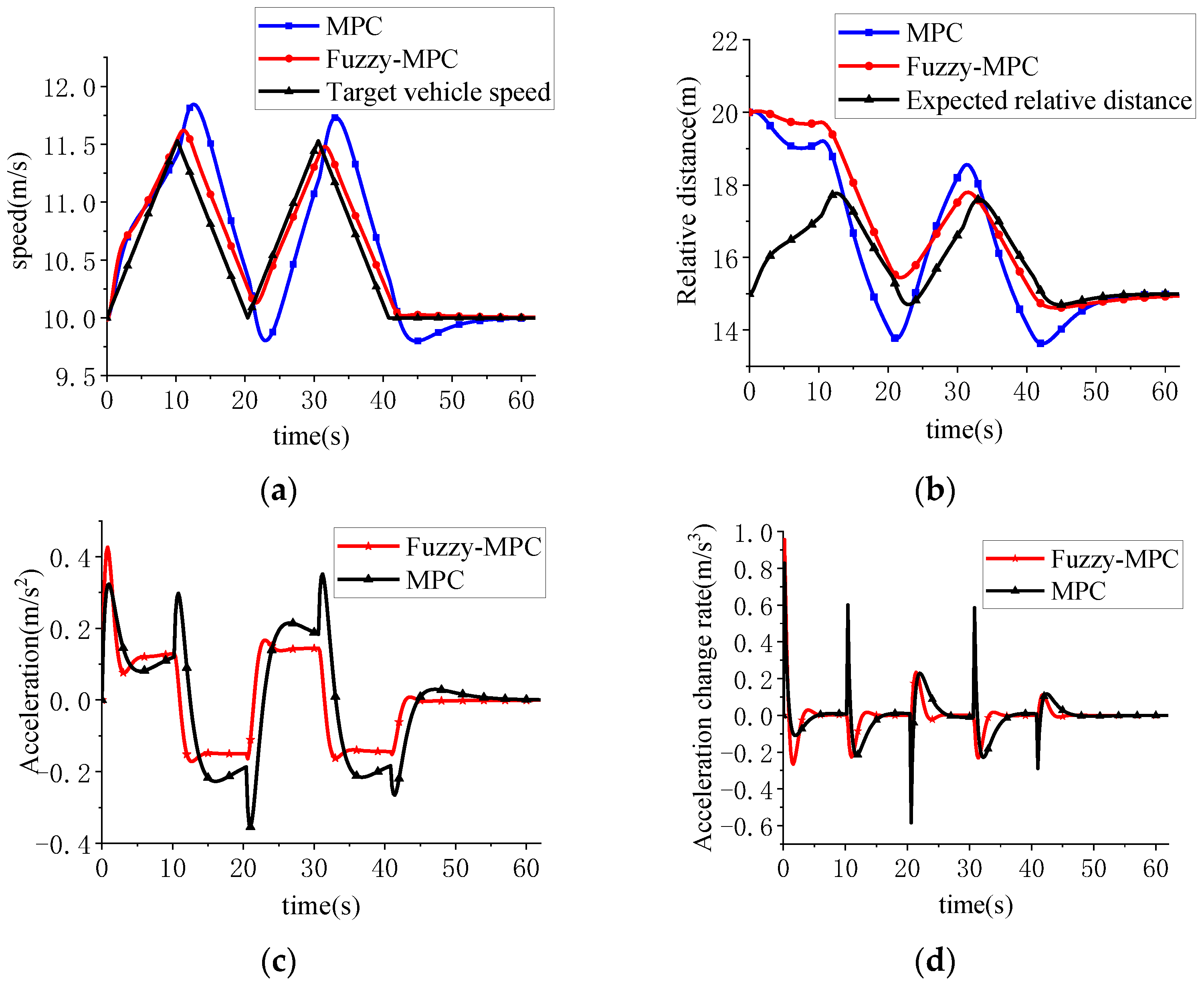
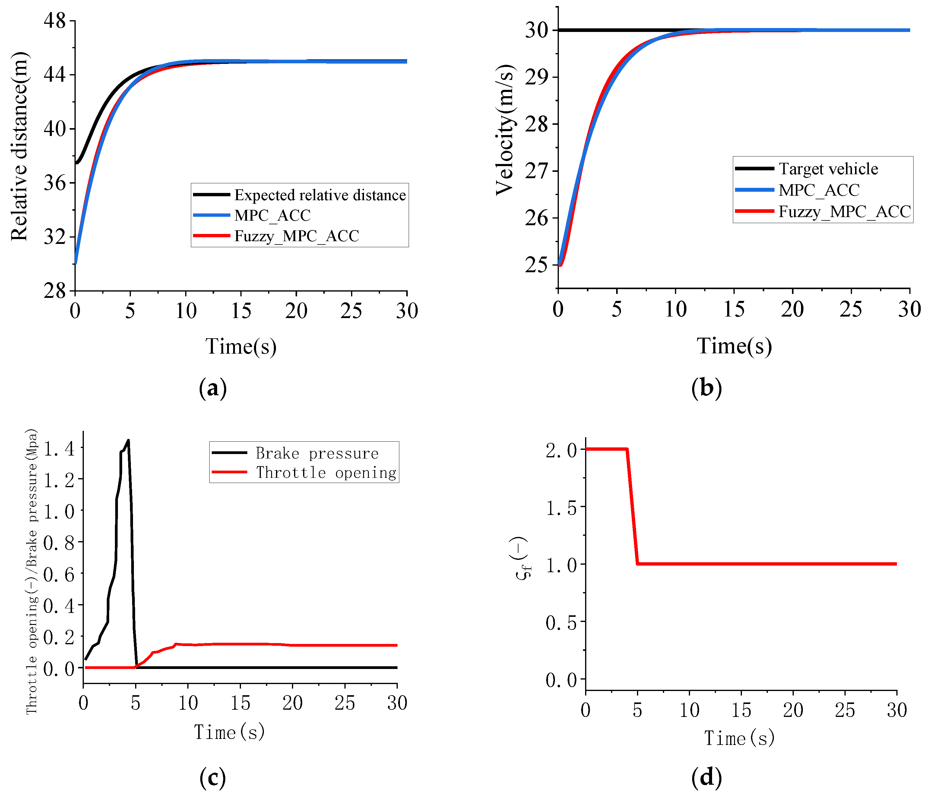
2.4.1. Normal Condition

The speed between the ACC vehicle and the target vehicle is 10 m/s. The target vehicle performs acceleration and deceleration movement, the initial distance between the two vehicles is 20 m and the simulation results are shown in Figure 3.
It can be seen from Figure 3a that in the working condition of frequent shifting of the preceding vehicle, Fuzzy-MPC has faster response and smaller error than traditional MPC. Figure 3b shows that the actual relative distance error of Fuzzy-MPC is smaller than that of traditional MPC. Figure 3c,d shows that the acceleration of Fuzzy-MPC is more stable, and the fluctuation of the acceleration rate is smaller, indicating that the Fuzzy-MPC has better followability, comfort and fuel economy.

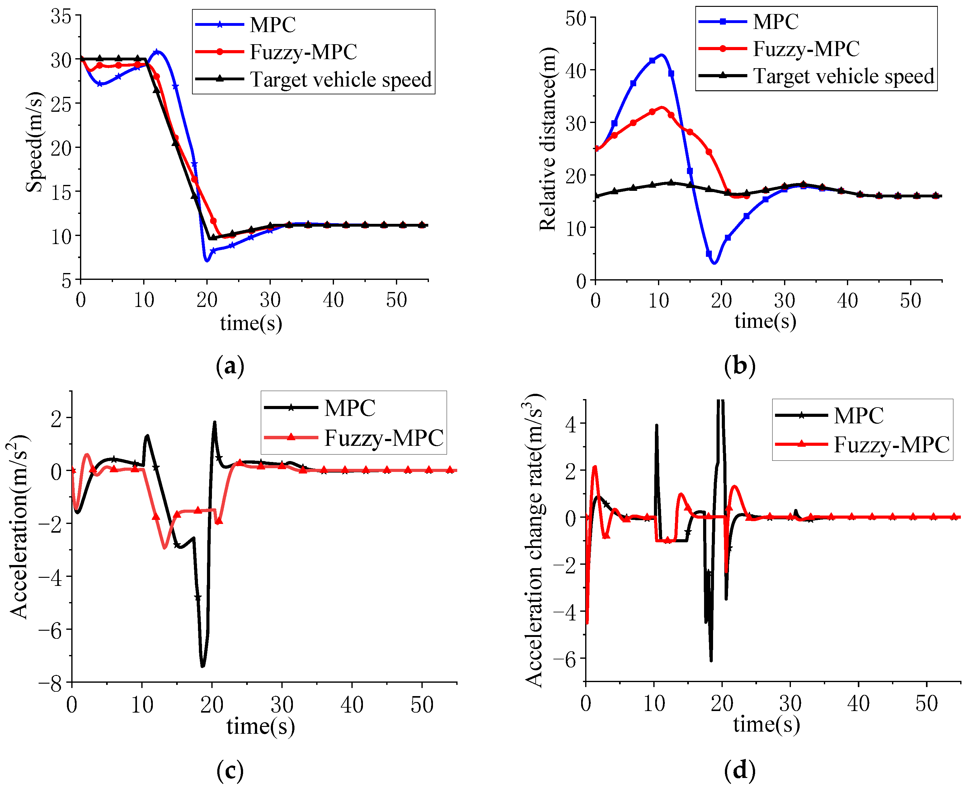
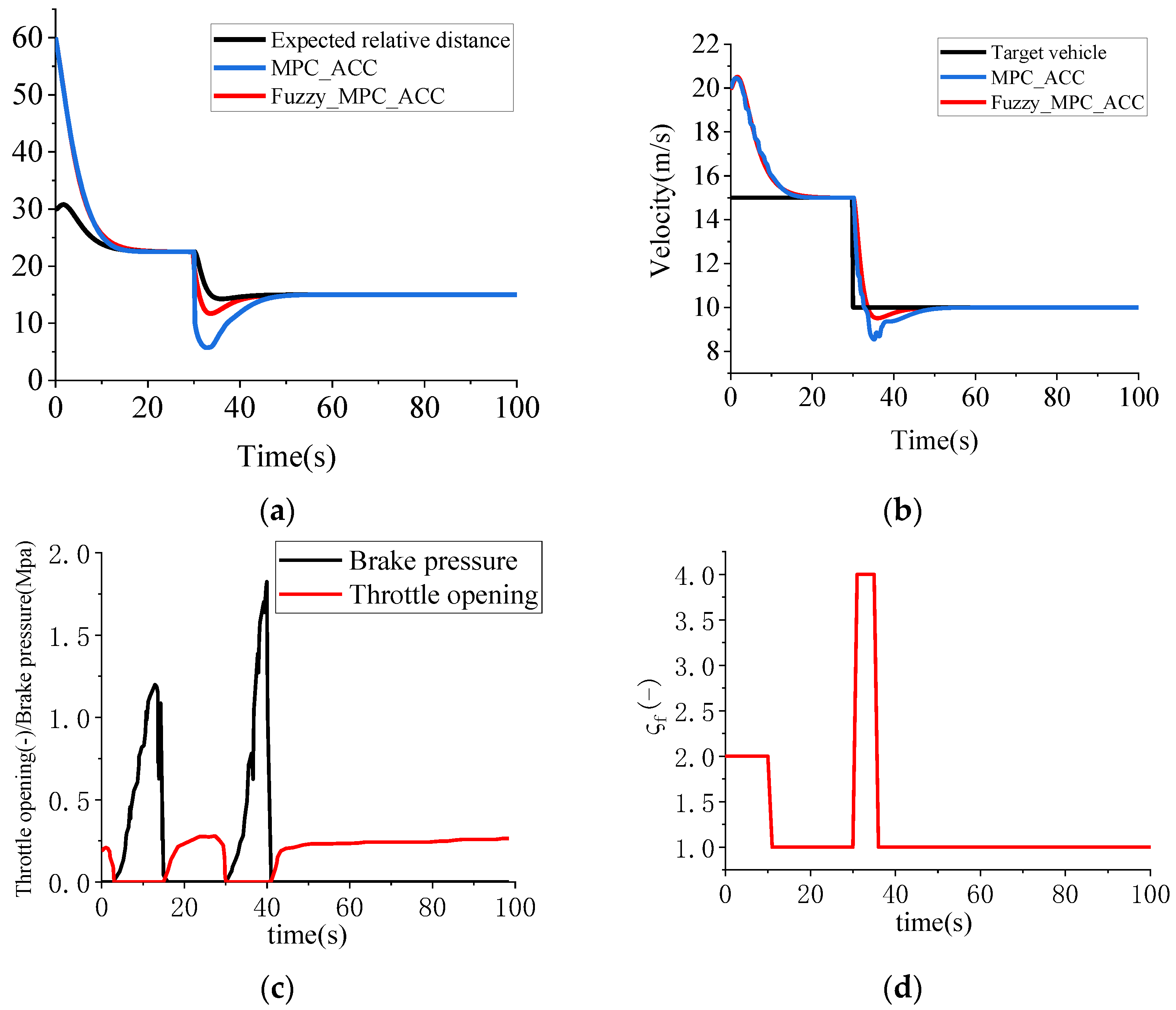
2.4.2. Emergency Conditions

Set the speed of both the ACC vehicle and the target vehicle to 30 m/s. At the 5th second, the target vehicle brakes at a deceleration of −2 m/s2. The initial relative distance between the two vehicles is 25 m. The simulation results are shown in Figure 4.
It can be seen from Figure 4a that Fuzzy-MPC is faster than the traditional MPC algorithm in terms of response. Figure 4b,c shows that the acceleration and acceleration change rate curve of the Fuzzy-MPC algorithm are more stable, which improves fuel economy and car following performance to a certain degree. In Figure 4d, the change range of the acceleration change rate of the Fuzzy-MPC is smaller, which improves comfort to a certain degree.
From the above simulation results, it can be seen that the ACC system control algorithm based on Fuzzy-MPC performs better than the traditional MPC under two working conditions, which not only ensures the safety of the vehicle, but also effectively improves the comfort and the fuel economy of the vehicle during driving.

3. Lower Controller Design

The lower controller calculates the throttle opening and brake pressure of the vehicle according to the output of the upper controller, so that the actual acceleration of the vehicle can track the expected acceleration, thereby achieving hierarchical control.

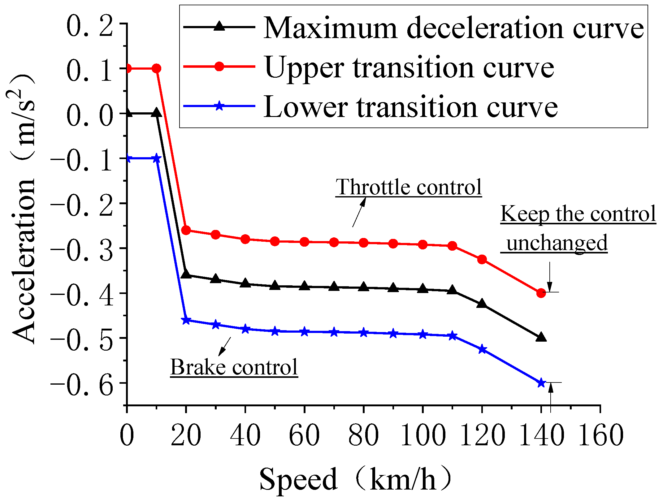
3.1. Throttle/Brake Switching Strategy

Frequent acceleration or deceleration of the vehicle not only damages the reliability of the corresponding parts of the vehicle, but it is also detrimental to the comfort of the drivers and passengers. To reduce this switching operation, the maximum deceleration reached at different vehicle speeds was measured when the vehicle was traveling freely in CarSim and plotted as a curve. To prevent frequent switching of the two systems, a transition area is set on both sides of the curve with a width of 2∆h and ∆h = 0.1, as shown in Figure 5.
Define the desired acceleration output by the upper controller as a d e s . According to the logical switching curve, when a ( 0 ) Δ h a d e s a ( 0 ) + Δ h , it keeps the previous state; when a d e s a ( 0 ) + Δ h , it is throttle control; when a d e s a ( 0 ) Δ h , it is brake control.

3.2. Throttle Control

This article uses an experimental method to simulate the vehicle model selected in CarSim. The initial speed of the vehicle is from 0 km/h to 120 km/h, and the throttle opening required to achieve different accelerations at different vehicle speeds is tested, as shown in Table 3.

3.3. Brake Control

When the vehicle needs to decelerate, the control mode is switched to brake control. Firstly, obtain the desired braking torque through a d e s . Secondly, obtain the desired brake pressure P d e s through the reverse brake model. Finally, the vehicle dynamics system will perform braking control according to the desired braking pressure P d e s .
When the vehicle is under braking conditions, the driving force is zero. The force analysis of the vehicle shows that the total resistance of the vehicle is F r .
F r = 1 2 C D A ρ v 2 + M g f
where C D is the coefficient of air resistance, A is the windward area, ρ is the density of your air, M is the mass of the vehicle, g is the acceleration of gravity, and f is the rolling resistance coefficient.
Under braking conditions, when the braking force F b r is less than the maximum braking force on the road, the braking force and braking pressure can satisfy the following relationship.
F b r = K b   P d e s
where K b   is the ratio of braking force to braking pressure and P d e s is the braking pressure.
Through simulation in CarSim, K b = 1582.3 can be obtained. According to Newton’s second law, by combining Equations (8) and (9), the following can be obtained.
P d e s = | M a d e s 1 2 C D A ρ v 2 M g f | K b

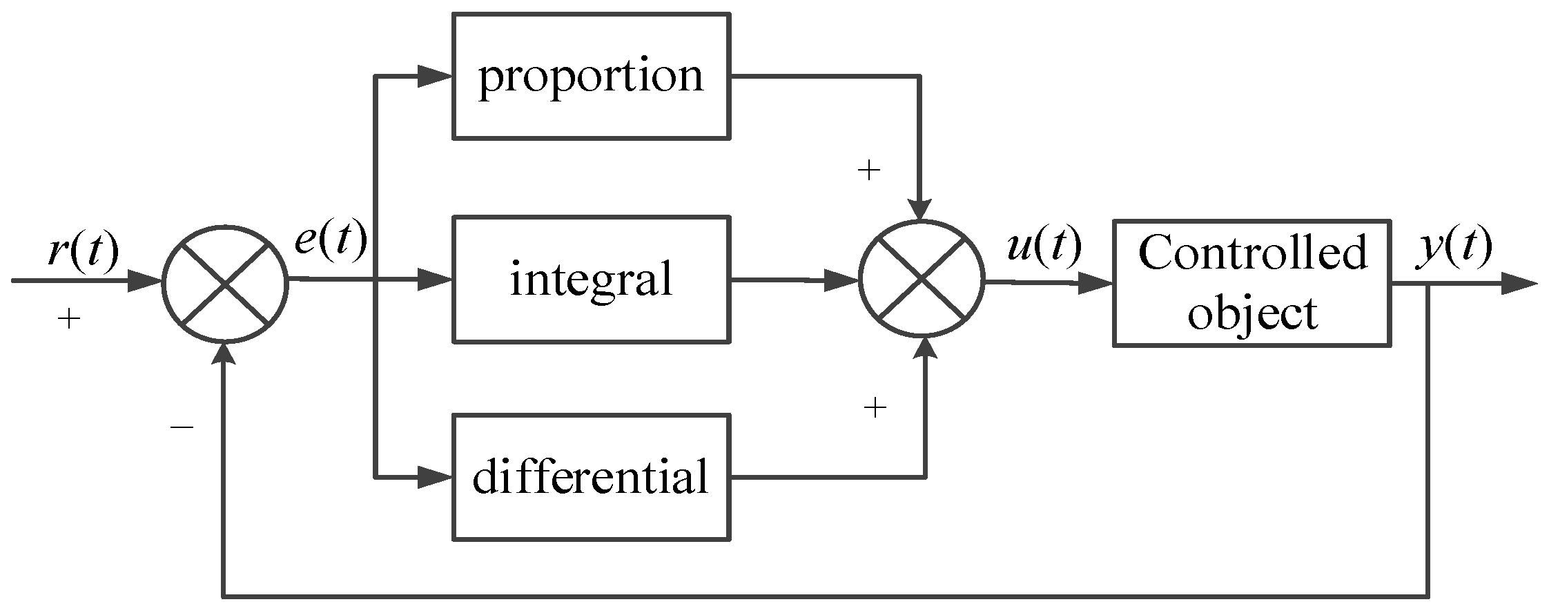
3.4. Design of Lower Controller Based on PID

To eliminate the error between the vehicle inverse dynamics model and the actual vehicle model, feedback control is used to adjust and improve the accuracy of the system model, as shown in Figure 6.
Among them, e ( t ) is the error value between the expected acceleration a d e s and the actual acceleration a .
e ( t ) = a d e s a
The PID control law is as follows.
u ( t ) = k p e ( t ) + k i   0 t e ( t ) d t + k d d e ( t ) d t
It can then be converted to a transfer function form, as shown in Equation (13).
G ( s ) = U ( s ) E ( s ) = k p + k i s + k d s
where u ( t ) is the output, k p is the proportional coefficient, k i is the integral coefficient, k d is the differential coefficient and s is the time.

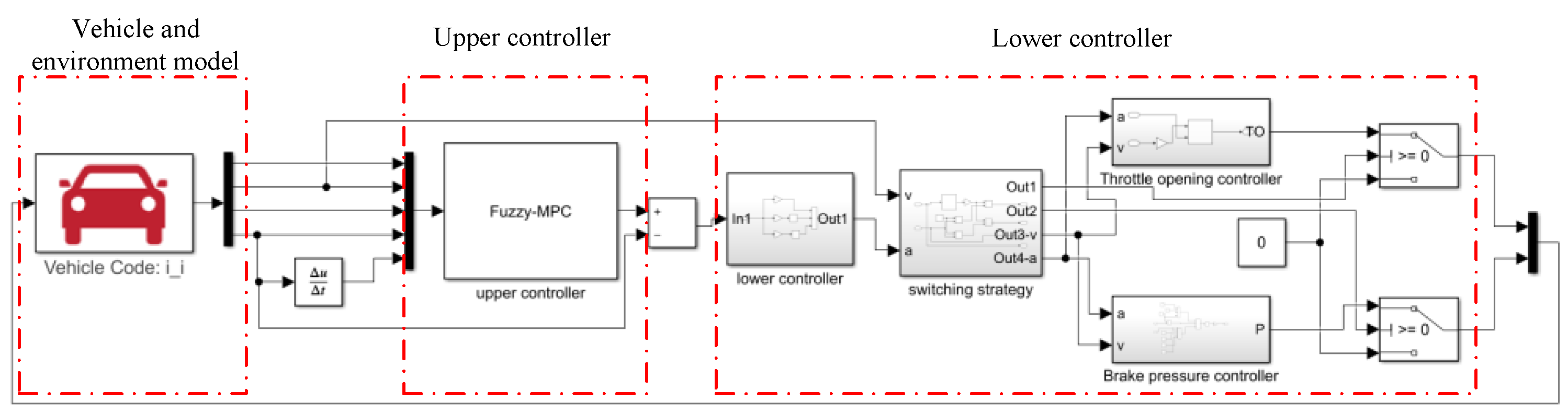
4. Co-Simulation Verification and Analysis

To verify the effectiveness of the algorithm, MATLAB/Simulink and CarSim are used for co-simulation. Build the lower controller, braking controller and throttle opening controller in Simulink. This is shown in Figure 7. Three following conditions are selected to compare the ACC vehicle based on MPC (MPC_ACC) and the ACC vehicle based on Fuzzy-MPC (Fuzzy_MPC_ACC). The simulation parameters are shown in Table 3.

4.1. Follow the Vehicle Smoothly

The initial speed of ACC in this working condition is 25 m/s. The target vehicle is 30 m ahead of the ACC and travels at a constant speed of 30 m/s. The simulation results are shown in Figure 8.
As shown in Figure 8a,b, when the actual relative distance is greater than the expected relative distance, the ACC vehicle starts to accelerate uniformly. At the 10th second, the speed of the ACC vehicle is equal to the speed of the target vehicle, and the actual relative distance and the expected relative distance slowly converge. Throttle opening/braking pressure is shown in Figure 8c, with a reverse reaction time of 5 s. As shown in Figure 8d, the change of ς f in the whole process shows that the safety of following the vehicle is emphasized in the first 5 s. As can be seen from the Figure 8, under this condition, the effect of on-line adjustment of the weight parameters of Fuzzy_MPC_ACC is similar to that of the fixed weight parameters of MPC_ACC. Both can safely and effectively track the front vehicle, but Fuzzy_MPC_ACC follows the front vehicle slightly faster than MPC_ACC.

4.2. Target Vehicle Insertion

The initial distance between the two vehicles is 60 m, the speed of the ACC vehicle is 20 m/s, and the speed of the target vehicle is 15 m/s. When the target vehicle is inserted at t = 30 s, the actual distance between the two vehicles becomes 10 m. The target vehicle has a speed of 10 m/s and is in a state of uniform motion. The simulation results are shown in Figure 9.
In Figure 9a,b, the ACC decelerates at the beginning to follow the target vehicle. At the 10th second, the speeds of the two vehicles are close, and the distance error between the two vehicles tends to zero. At 30 s, the target vehicle cuts in and the actual distance between the two vehicles becomes 10 m. To ensure driving safety, the ACC continues to decelerate and can smoothly keep up with the vehicle in front in 40 s. From the two figures, it can be seen that in the deceleration stage of the vehicle after the vehicle in front is inserted, Fuzzy_MPC_ACC is more adaptable than MPC_ACC and the minimum value of relative distance is larger, the speed changes more gently, and it becomes safer and more comfortable. Figure 9c shows that the throttle opening and braking force change reasonably. Figure 9d shows that ACC tends to be safer in the deceleration section, and more comfortable with greater fuel economy in the smooth following section.

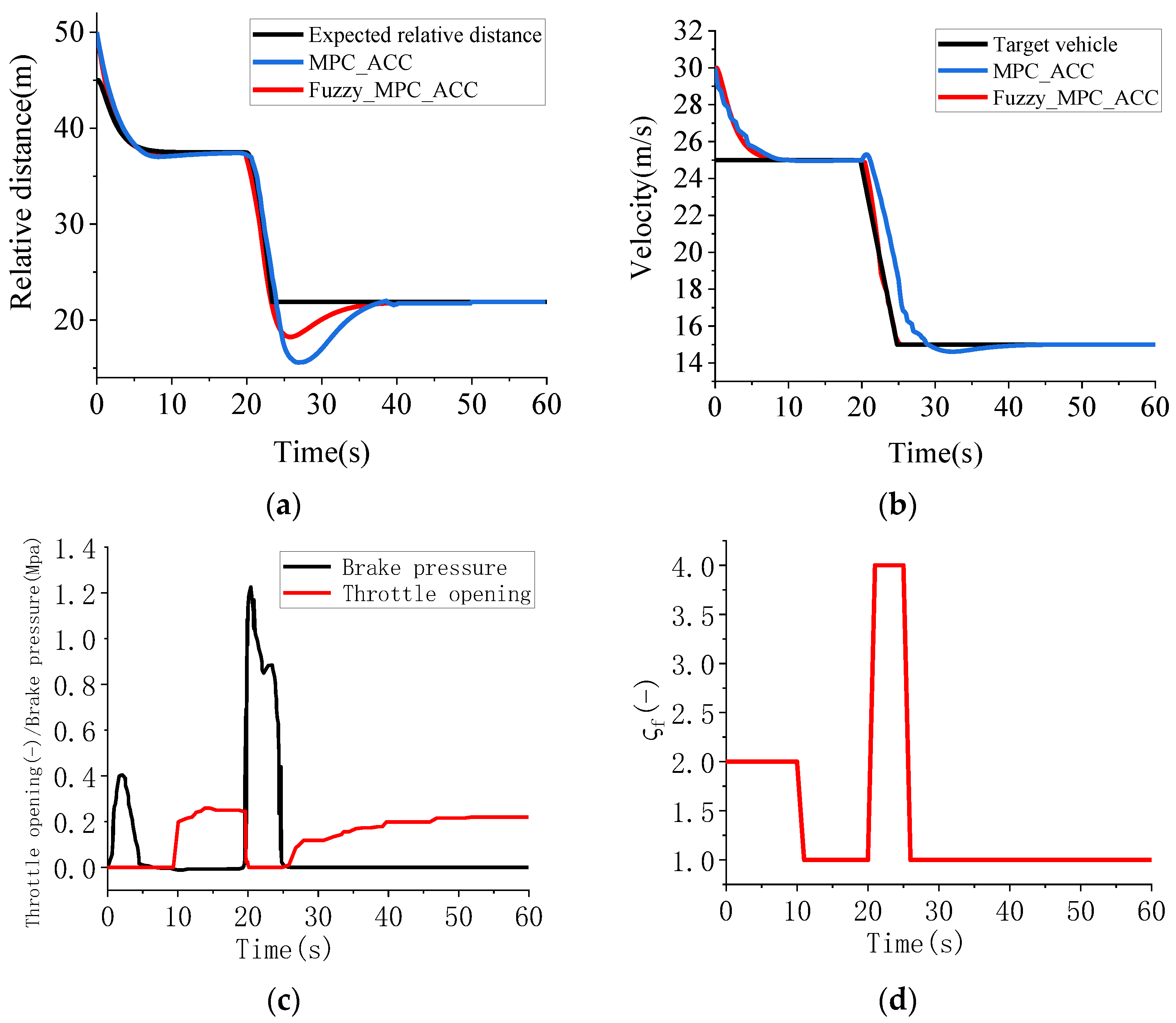
4.3. Emergency Braking

The initial speed of ACC is 30 m/s. The target vehicle travels at a constant speed of 25 m/s, and suddenly brakes with an acceleration of −2 m/s2 at the 20th second and continues for 5 s and then maintains a constant speed. The simulation results are shown in Figure 10.
In Figure 10a,b, the ACC decelerates at the beginning to follow the target vehicle, and the distance between the two vehicles gradually approaches the actual value. At the 10th second, the speeds of the two vehicles tend to be the same, and the distance between them tends towards the expected value. At the 20 s point, the target vehicle brakes abruptly, and the ACC also performs an emergency brake, which effectively avoids rear-end collisions and ensures the safety of the vehicle. As can be seen from the two figures, since the minimum relative distance of Fuzzy_MPC_ACC is greater than that of MPC_ACC, the speed change is smoother, and Fuzzy_MPC_ACC can track the vehicle in front more quickly and safely. Figure 10c shows that the lower controller has a better first response. Figure 10d shows that there are higher requirements for safety when the target vehicle brakes in an emergency.

5. Conclusions

In order to improve the driving performance of ACC system in complex conditions, a Fuzzy-MPC algorithm is proposed. Based on the longitudinal kinematics model of two vehicles, the online variable weight Fuzzy-MPC algorithm is simulated. In the numerical simulation, the speed, relative distance, acceleration and acceleration change rate of the vehicle under normal and emergency conditions are calculated. The results show that, compared with the traditional MPC algorithm, the Fuzzy-MPC algorithm can follow the vehicle more quickly and stably when the driving condition changes, and has better safety, comfort and fuel economy. Combined with the mathematical model, control algorithm and low controller, the co-simulation of CarSim is carried out under the conditions of smooth following of the vehicle, target vehicle insertion and emergency braking. It is found that the changes of speed, relative distance and throttle opening/brake pressure are stable under the three working conditions.

Author Contributions

Conceptualization, J.M., L.Y. and Y.H.; methodology, J.M., L.Y.; software, J.M., L.Y. and Y.H.; validation, J.M., L.Y. and Y.H.; formal analysis, K.L. and J.D.; investigation, L.Y.; resources, J.M., K.L. and J.D.; data curation Y.H.; writing—original draft preparation, L.Y. and Y.H.; writing—review and editing, J.M.; visualization, L.Y.; supervision, J.M., K.L. and J.D. All authors have read and agreed to the published version of the manuscript.

Funding

This work was supported in part by the National Natural Science Foundation of China (Grant No. 61701397 and Grant No. 51705419), and in part by the Fundamental Research Funds for the Central Universities, CHD (Grant No. 300102210512 and 300102210511).

Institutional Review Board Statement

Not applicable.

Informed Consent Statement

Not applicable.

Data Availability Statement

Not applicable.

Acknowledgments

We acknowledge the support provided to this study by Xi’an University of Technology, Xi’an University of Technology in the form of time and facilities.

Conflicts of Interest

The authors declare no conflict of interest.

References

  1. Xiao, L.; Gao, F. A comprehensive review of the development of adaptive cruise control systems. Veh. Syst. Dyn. 2010, 48, 1167–1192. [Google Scholar] [CrossRef]
  2. Vahidi, A.; Eskandarian, A. Research advances in intelligent collision cruise control systems. IEEE Trans. Intell. Transp. Syst. 2003, 4, 143–153. [Google Scholar] [CrossRef] [Green Version]
  3. Jianlong, Z.; Ioannou, P.A. Longitudinal control of heavy trucks in mixed traffic: Environmental and fuel economy considerations. IEEE Trans. Intell. Transp. Syst. 2006, 7, 92–104. [Google Scholar]
  4. Chan, Y.F.; Moallem, M.; Wang, W. Efficient implementation of PID control algorithm using FPGA technology. In Proceedings of the IEEE Conference on Decision and Control (CDC), Nassau, Bahamas, 16 May 2005. [Google Scholar]
  5. Canale, M.; Malan, S. Tuning of stop and go driving control strategies using driver behaviour analysis. In Proceedings of the IEEE Intelligent Vehicle Symposium, Versailles, France, 17–21 June 2002; pp. 407–412. [Google Scholar]
  6. Corona, D.; Lazar, M.; Schutter, B.D.; Heemels, M. A hybrid MPC approach to the design of a smart adaptive cruise controller. In Proceedings of the 2006 IEEE Conference on Computer Aided Control System Design, Munich, Germany, 4–6 October 2006. [Google Scholar]
  7. Naus, G.; Ploeg, J.; Van De Molengraft, R.; Steinbuch, M. Explicit MPC design and performance-based tuning of an adaptive cruise control stop-&-go. In Proceedings of the Intelligent Vehicles Symposium, Eindhoven, The Netherlands, 4–6 June 2008. [Google Scholar]
  8. Firoozi, R.; Nazari, S.; Guanetti, J.; O’Gorman, R.; Borrelli, F. Safe adaptive cruise control with road grade preview and V2V communication. arXiv 2018, arXiv:1810.09000. [Google Scholar]
  9. Tran, A.T.; Sakamoto, N.; Suzuki, T. A combination of analytical and model predictive optimal methods for adaptive cruise control problem. In Proceedings of the 2018 Australian & New Zealand Control Conference (ANZCC), Melbourne, Australia, 7–8 December 2018. [Google Scholar]
  10. Eom, H.; Lee, S.H. Human-automation interaction design for adaptive cruise control systems of ground vehicles. Sensors 2015, 15, 13916–13944. [Google Scholar] [CrossRef] [PubMed] [Green Version]
  11. Subiantoro, A.; Muzakir, F.; Yusivar, F. Adaptive cruise control based on multistage predictive control approach. In Proceedings of the International Conference on Nano Electronics Research and Education, Hamamatsu, Japan, 27–29 November 2018. [Google Scholar]
  12. Liu, H.; Miao, C.; Zhu, G.G. Economic adaptive cruise control for a power split hybrid electric vehicle. IEEE Trans. Intell. Transp. Syst. 2019, 21, 4161–4170. [Google Scholar] [CrossRef]
  13. Zhao, S.; Zhang, K. A distributionally robust stochastic optimization-based model predictive control with distributionally robust chance constraints for cooperative adaptive cruise control under uncertain traffic conditions. Transp. Res. Part B Methodol. 2020, 138, 144–178. [Google Scholar] [CrossRef]
  14. Wu, W.; Zou, D.; Ou, J.; Hu, L. Adaptive cruise control strategy design with optimized active braking control algorithm. Math. Probl. Eng. 2020, 2020. [Google Scholar] [CrossRef]
  15. Jiang, J.; Ding, F.; Wu, J.; Tan, H. A personalized human drivers’ risk sensitive characteristics depicting stochastic optimal control algorithm for adaptive cruise control. IEEE Access 2020, 8, 145056–145066. [Google Scholar] [CrossRef]
  16. Kuragaki, S.; Kuroda, H.; Minowa, T.C. An adaptive control using wheel torque management technique. SAE Tech. Pap. 1998. [Google Scholar] [CrossRef]
  17. Yi, K.; Hong, J.; Kwon, Y.D. A vehicle control algorithm for stop-and-go cruise control. Proc. Inst. Mech. Eng. Part D J. Automob. Eng. 2001, 215, 1099–1115. [Google Scholar] [CrossRef]
  18. Broqua, F. Cooperative driving: Basic concepts and a first assessment of the intelligent cruise control strategies. In Proceedings of the DRIVE Conference, Brussels, Belgium, 4–6 February 1991; pp. 908–929. [Google Scholar]
  19. Li, X.; Zhang, X.; Zou, Y.; Zhang, T.; Wei, S. A research on the adaptive cruise controller for electric bus. In Society of Automotive Engineers (SAE)–China Congress; Springer: Singapore, 2018; pp. 415–432. [Google Scholar]
  20. Zhang, S.; Zhuan, X. Study on adaptive cruise control strategy for battery electric vehicle. Math. Probl. Eng. 2019, 2019. [Google Scholar] [CrossRef] [Green Version]
  21. Cheng, S.; Li, L.; Mei, M.M.; Nie, Y.-L.; Zhao, L. Multiple-objective adaptive cruise control system integrated with DYC. IEEE Trans. Veh. Technol. 2019, 68, 4550–4559. [Google Scholar] [CrossRef]
  22. David, J.; Brom, P.; Stary, F.; Bradáč, J.; Dynybyl, V. Application of artifitial neural networks to streamline the process of adaptive cruise control. Sustainability 2021, 13, 4572. [Google Scholar] [CrossRef]
  23. Luo, L.H.; Liu, H.; Li, P.; Wang, H. Model predictive control for adaptive cruise control with multi-objectives: Comfort, fuel-economy, safety and car-following. J. Zhejiang Univ. Sci. A Appl. Phys. Eng. 2010, 11, 191–201. [Google Scholar] [CrossRef]
  24. Zhang, J.H.; Li, Q.; Chen, D.P. Drivers imitated multi-objective adaptive cruise control algorithm. Control Theory Appl. 2018, 35, 769–777. [Google Scholar]
Figure 1. Schematic diagram of longitudinal kinematics. where x p is the target vehicle position, x f is the ACC vehicle position, and d is the actual relative distance between the two vehicles.
Machines 09 00160 g001
Figure 2. Membership function of each variable: (a) relative distance d ; (b) relative speed v r e l ; (c) the weight coefficient c f .
Machines 09 00160 g002aMachines 09 00160 g002b
Figure 3. Stable follow: (a) speed; (b) relative distance; (c) acceleration; (d) acceleration change rate.
Machines 09 00160 g003
Figure 4. Emergency brake: (a) speed; (b) relative distance; (c) acceleration; (d) acceleration change rate.
Machines 09 00160 g004
Figure 5. Acceleration/braking switching curve.
Machines 09 00160 g005
Figure 6. PID control schematic diagram.
Machines 09 00160 g006
Figure 7. ACC system co-simulation environment establishment.
Machines 09 00160 g007
Figure 8. Acceleration conditions: (a) speed; (b) relative distance; (c) throttle opening/brake pressure; (d) weight coefficient ς f .
Machines 09 00160 g008
Figure 9. Target vehicle insertion: (a) speed; (b) relative distance; (c) throttle opening/brake pressure; (d) weight coefficient ς f .
Machines 09 00160 g009
Figure 10. Emergency braking: (a) speed; (b) relative distance; (c) throttle opening/brake pressure; (d) weight coefficient ς f .
Machines 09 00160 g010
Table 1. Fuzzy control rules.
dHEHCGDFCFE
vref
HEFEFEFWFCFC
HCFEFEFWFCFE
GDFEFEFCGDGD
FCFEFWFCGDGD
FEFWFCGDGDGD
Table 2. Simulation parameter table.
ParameterValueUnitParameterValueUnit
Ts0.2sumin−5.5m/s2
τ h 1s ξ max d 1-
τ 0.5m ξ min d 0-
d05m ξ max v f 1-
Np16- ξ min v f −1-
Nc5- ξ max a f 0.1-
vfmax35m/s ξ min a f −0.1-
vfmin0m/s ξ max j e r k 0-
afmax−5.5m/s2 ξ min j e r k 0-
afmin2.5m/s2 ξ max u 0.1-
jerkmax2.5m/s3 ξ min u −0.1-
jerkmin−2.5m/s3p1, p2, p3, p4, p53-
umax2.5m/s2w1, w2, w3, w4, w50.5-
Table 3. Two dimensional relationships of inverse engine model.
a ( m / s 2 )
v(km/h) −1011.522.534
0000.050.10.120.120.154
1000.10.120.120.130.150.180.2
2000.120.140.180.20.20.250.4
3000.120.170.20.250.30.350.5
4000.130.20.250.30.350.450.7
8000.150.30.450.50.711
12000.20.450.71111
Publisher’s Note: MDPI stays neutral with regard to jurisdictional claims in published maps and institutional affiliations.

