
Mathematical Validation of Experimentally Optimised Parameters Used in a Vibration-Based Machine-Learning Model for Fault Diagnosis in Rotating Machines


Abstract
:1. Introduction
2. Experimental Rig and Data
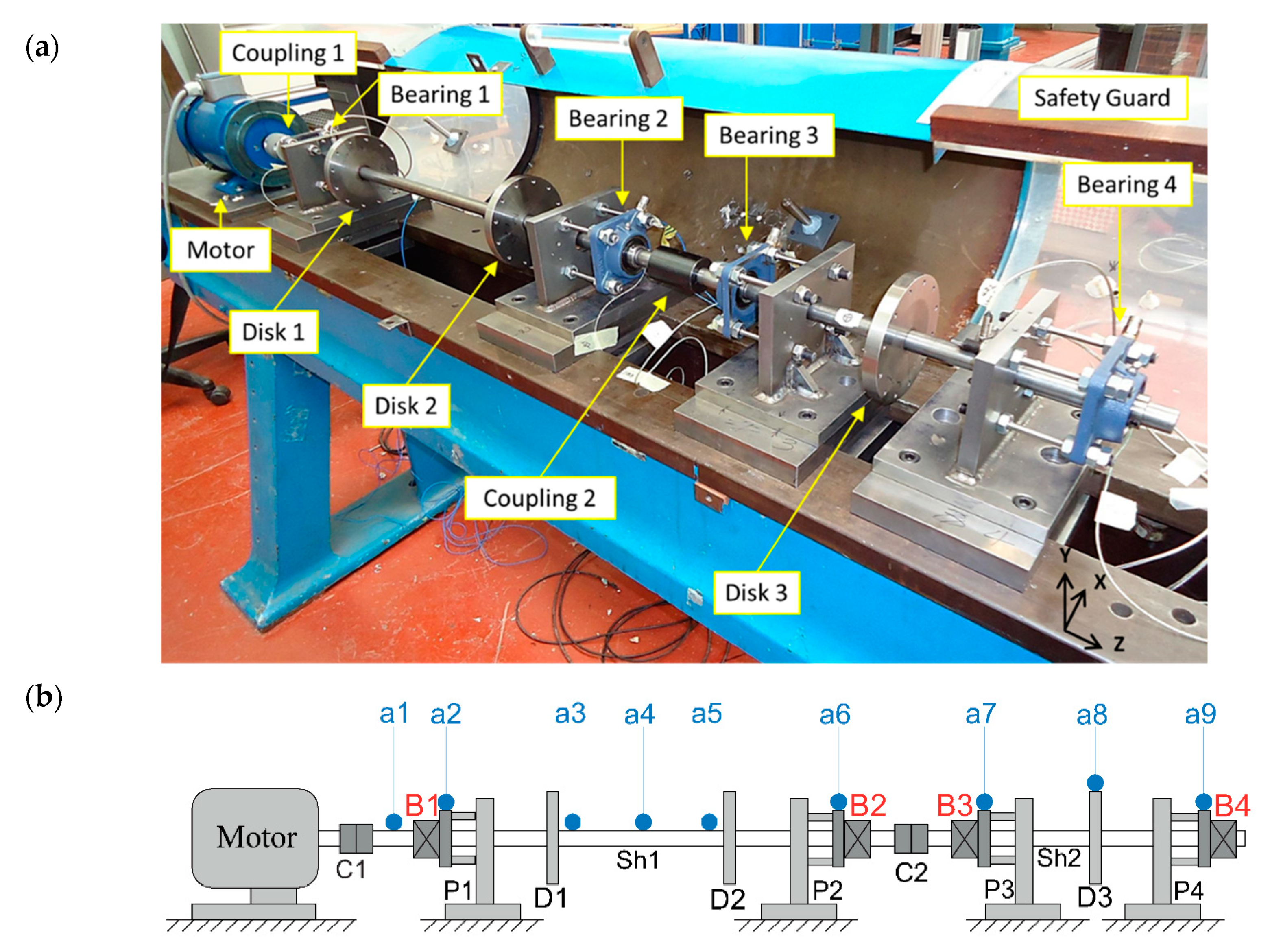
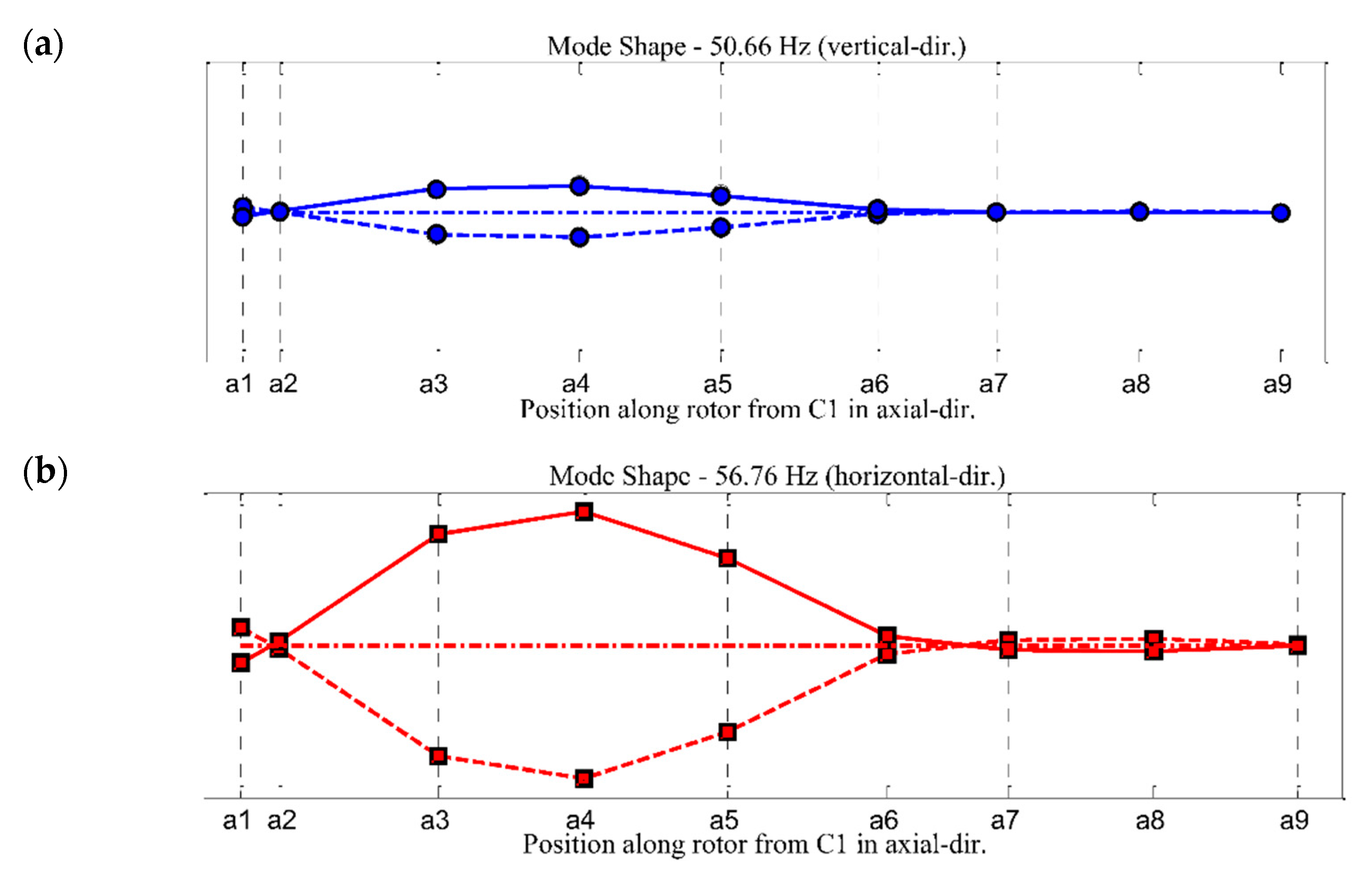
2.1. Experimental Rig and Mode Shapes
2.2. Experimental Data
3. Optimised Experimental Model
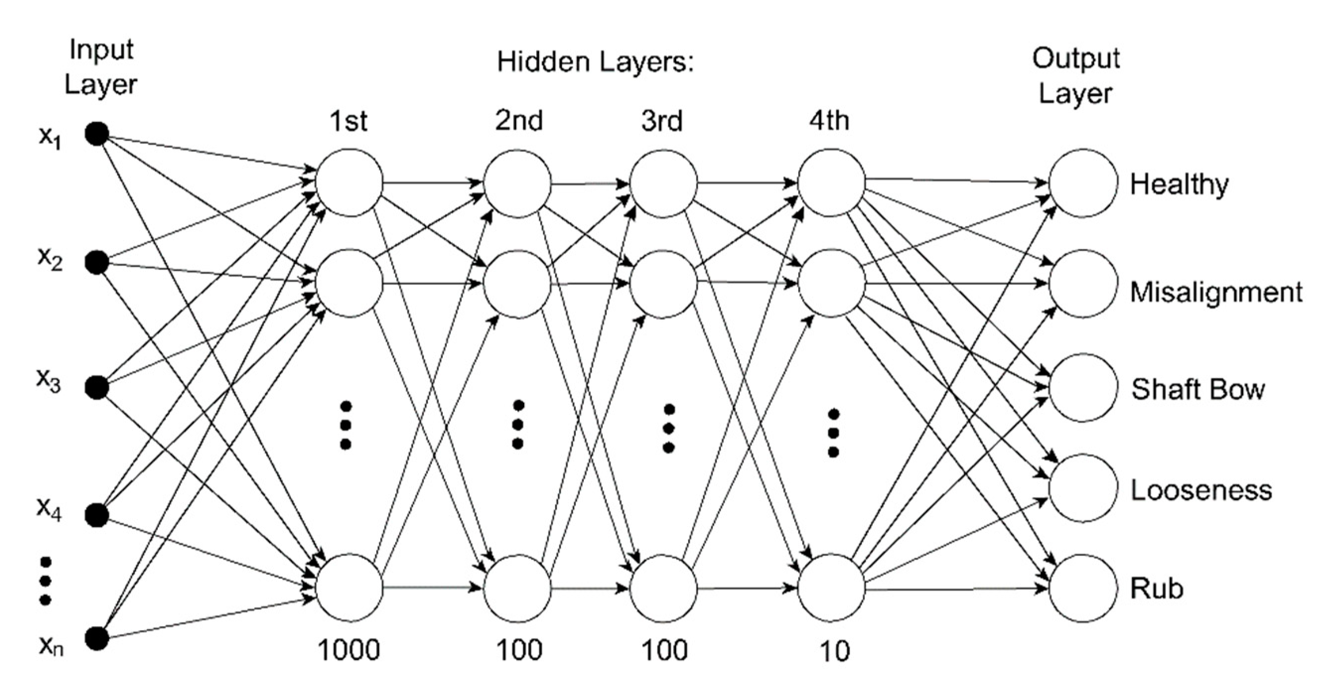
3.1. Vibration-Based Machine-Learning Model for the Fault Diagnosis in Rotating Machines
3.2. Results of Experimental Optimised Model
4. Finite-Element Model and Vibration Responses Estimation
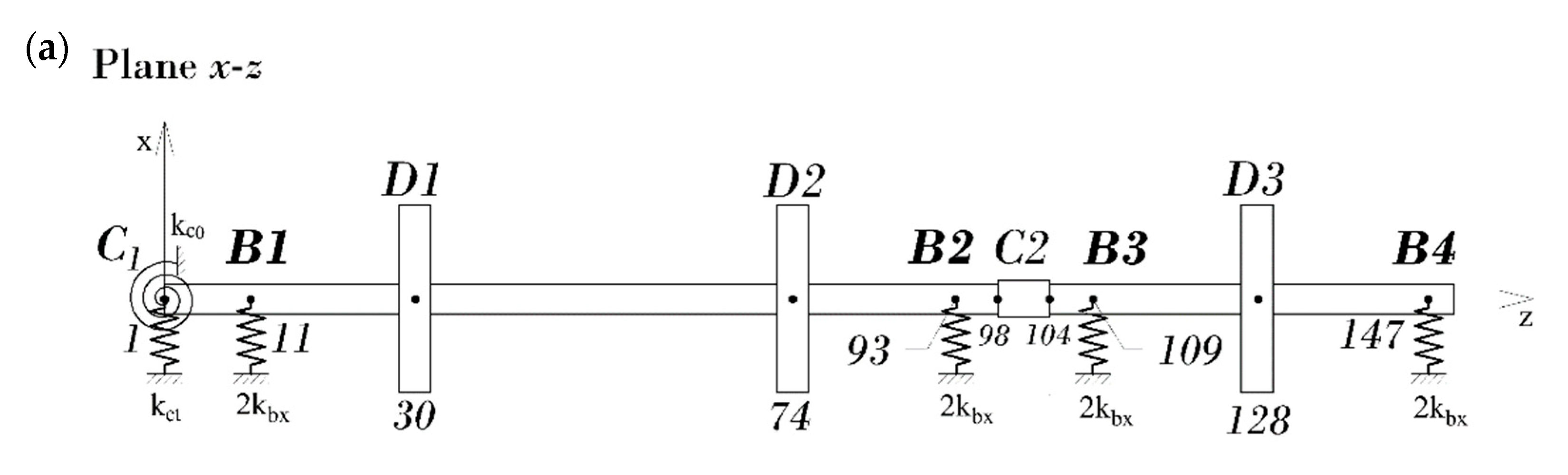
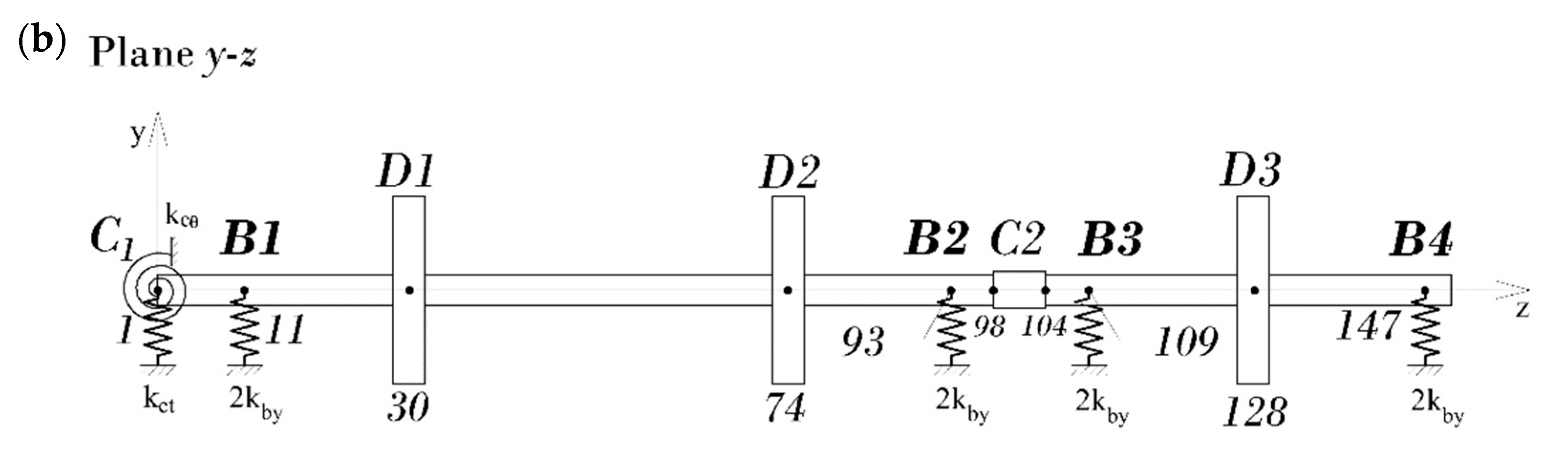
4.1. An FE Model and Mode Shapes
- Flexible coupling, C1: the flexible coupling between the rotor and the motor is used to remove the motor vibration influence on the rotor to maximum extent. Therefore, the coupling mass and stiffnesses are only added to Node 1 of the FE model to account the dynamics related to the rotor.
- Rigid coupling, C2: this element is modeled using the Timoshenko beam theory, as it is considered a rigid link in the central shaft-line model.
- Balancing discs, D1, D2, D3: the mass and gyroscopic matrices of the discs are added to Nodes 30, 74, and 128, respectively.
- Bearings and their pedestals: the mass and equivalent stiffnesses are added to respective Nodes, 11, 93, 109, and 147. The stiffness values at these locations are determined by iterations until the first and second natural frequencies known from the experimentally identified natural frequencies are matched.
4.2. Rotor Conditions Simulation
4.2.1. Healthy Rotor (Residual Unbalance)
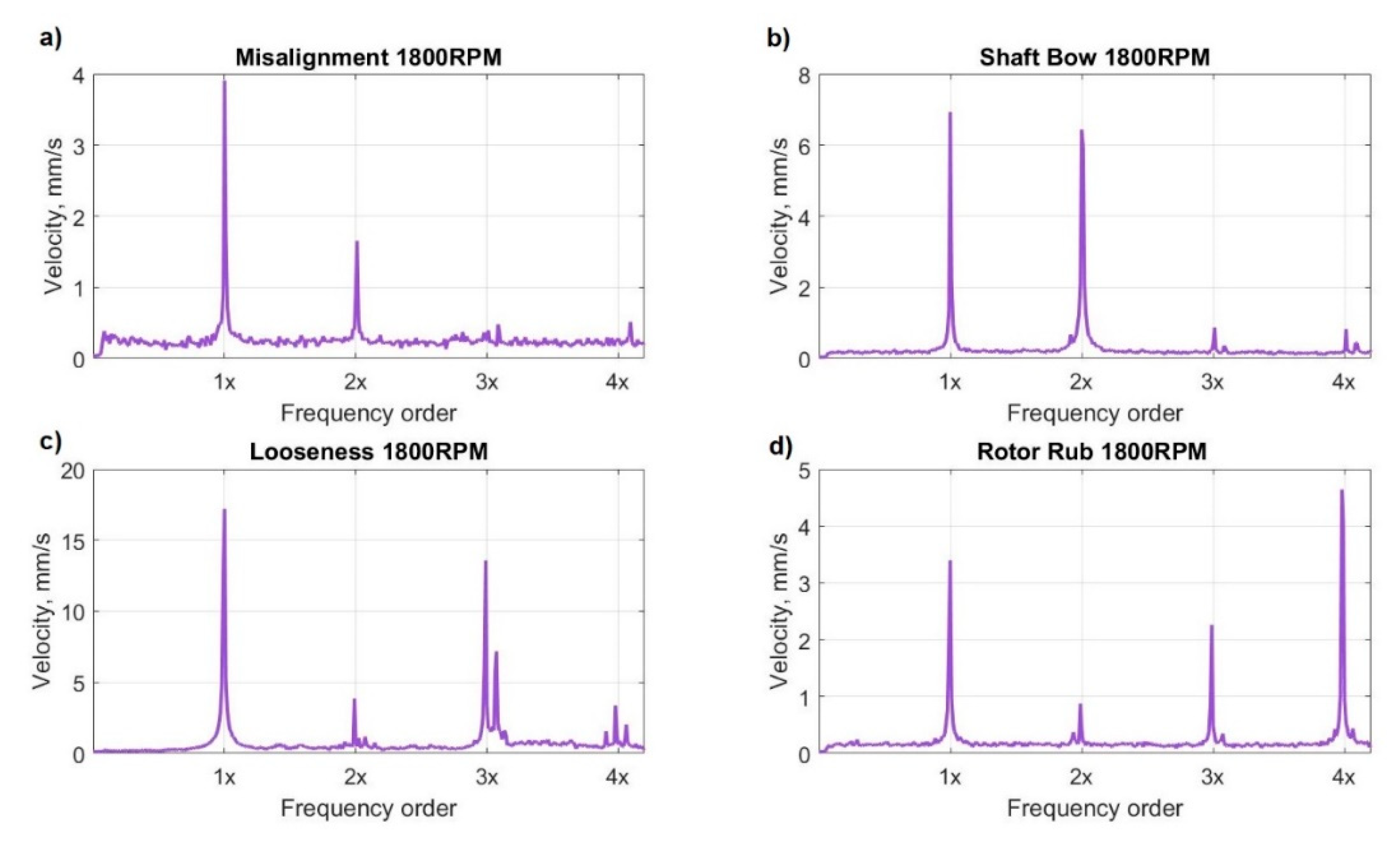
4.2.2. Misalignment
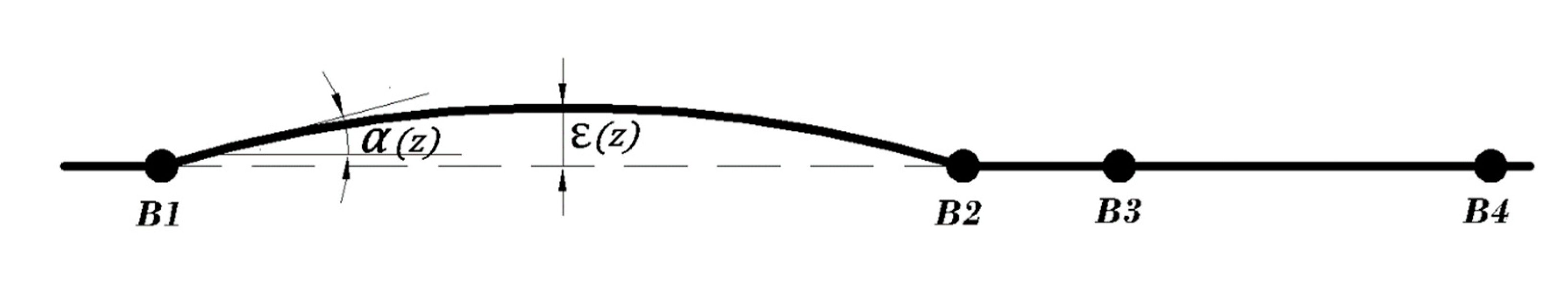
4.2.3. Shaft Bow
4.2.4. Looseness in Bearing Pedestal
4.2.5. Rotor Rub
- the displacement is lower or equal than the defined clearance in the vertical direction and free motion is observed in the rotor, then the equation of motion remains as Equation (4);
- displacement is higher than the clearance and contact exists between rotor and stator, increasing the stiffness due the stator effect. A high value of stator stiffness is defined, and the equation of motion is updated following the same considerations than in the looseness model, obtaining Equation (9). In this equation, represents the increment on stiffness and the forces, both due the contact.
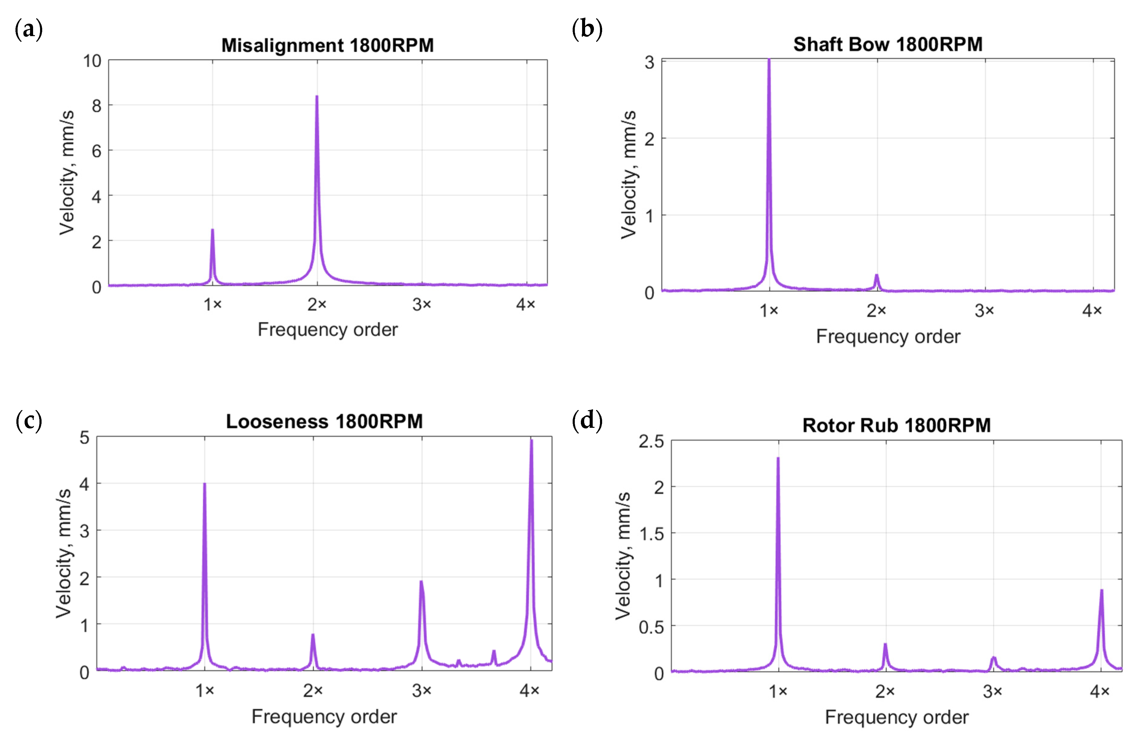
4.3. Responses Estimation
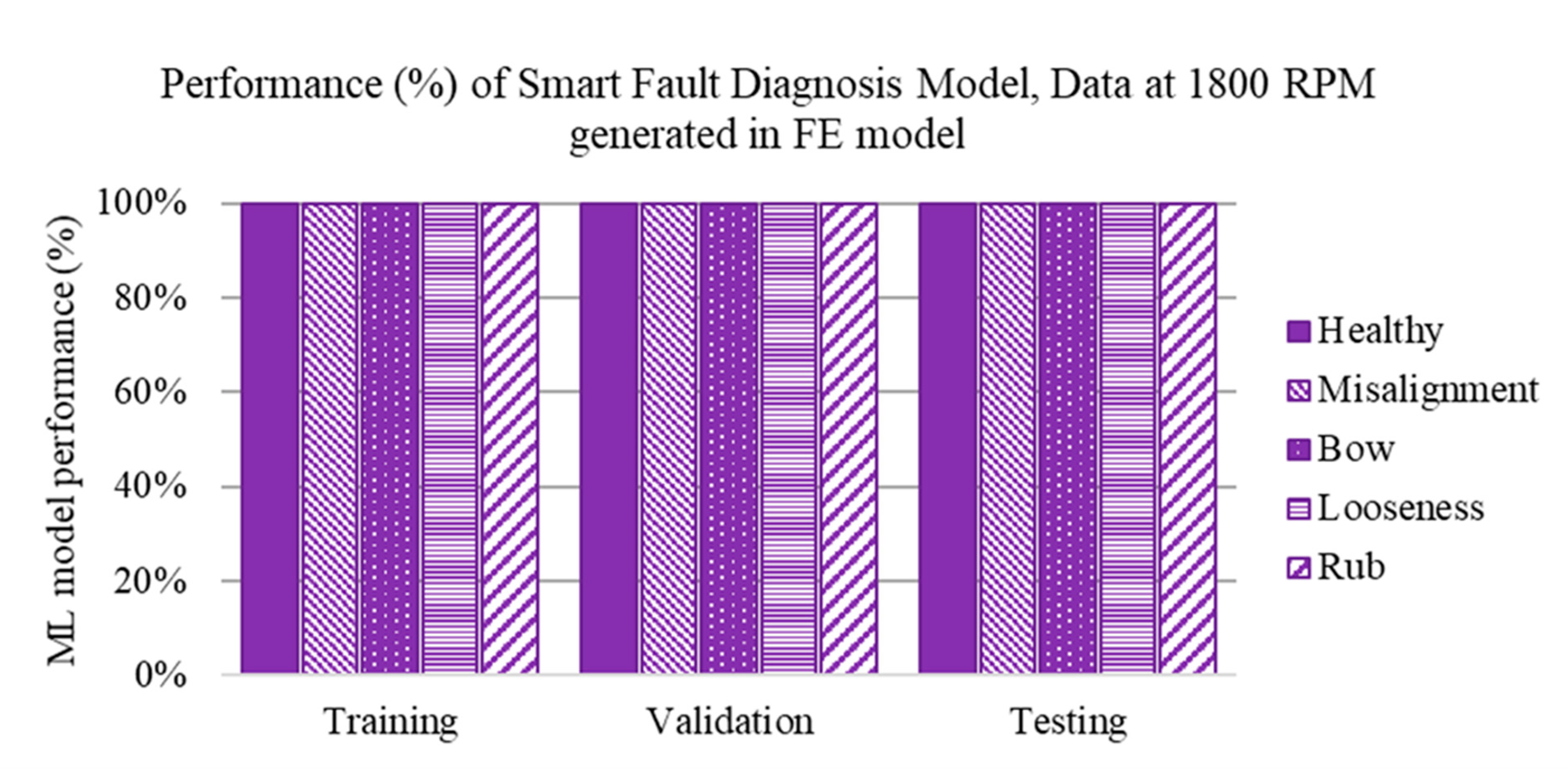
5. Mathematical Validation
5.1. Validation at 1800 RPM
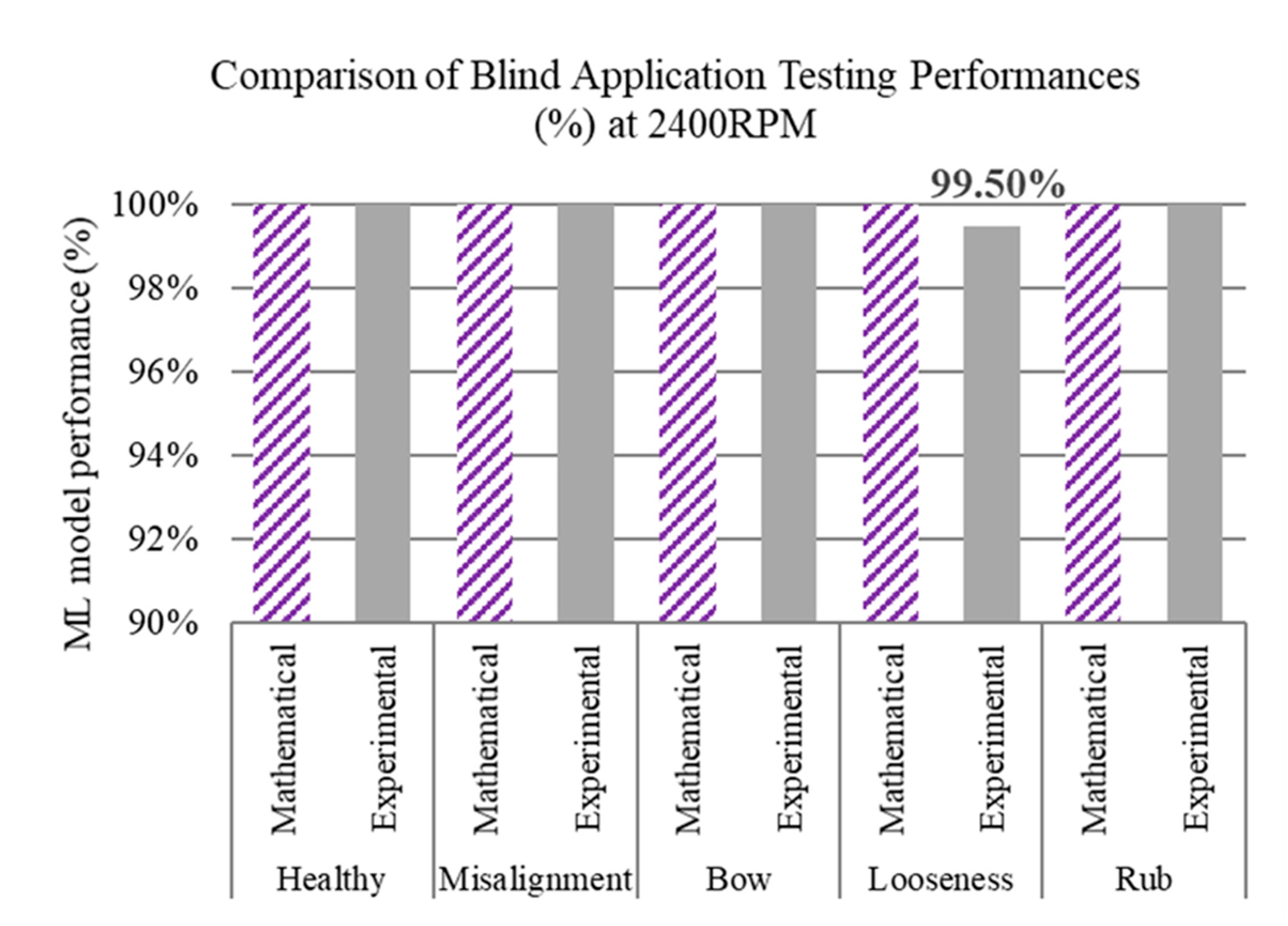
5.2. Validation of Blind Application
6. Concluding Remarks
Author Contributions
Funding
Acknowledgments
Conflicts of Interest
References
- Thiery, F.; Aidanpää, J.O. Nonlinear vibrations of a misaligned bladed Jeffcott rotor. Nonlinear Dyn. 2016, 86, 1807–1821. [Google Scholar] [CrossRef] [Green Version]
- Vlajic, N.; Champneys, A.R.; Balachandran, B. Nonlinear dynamics of a Jeffcott rotor with torsional deformations and rotor-stator contact. Int. J. Non. Linear. Mech. 2017, 92, 102–110. [Google Scholar] [CrossRef] [Green Version]
- Chávez, J.P.; Hamaneh, V.V.; Wiercigroch, M. Modelling and experimental verification of an asymmetric Jeffcott rotor with radial clearance. J. Sound Vib. 2015, 334, 86–97. [Google Scholar] [CrossRef]
- Guo, C.; Al-Shudeifat, M.A.; Yan, J.; Bergman, L.A.; McFarland, D.M.; Butcher, E.A. Application of empirical mode decomposition to a Jeffcott rotor with a breathing crack. J. Sound Vib. 2013, 332, 3881–3892. [Google Scholar] [CrossRef]
- Guo, C.; Yan, J.; Yang, W. Crack detection for a Jeffcott rotor with a transverse crack: An experimental investigation. Mech. Syst. Signal Process. 2017, 83, 260–271. [Google Scholar] [CrossRef]
- Gómez, M.J.; Castejón, C. Crack detection in rotating shafts based on 3× energy: Analytical and experimental analyses. MAMT 2016, 96, 94–106. [Google Scholar] [CrossRef]
- Singh, S.; Tiwari, R. Model-based switching-crack identification in a Jeffcott rotor with an offset disk integrated with an active magnetic bearing. J. Dyn. Syst. Meas. Control. Trans. ASME 2016, 138, 031006. [Google Scholar] [CrossRef]
- Heindel, S.; Becker, F.; Rinderknecht, S. Unbalance and resonance elimination with active bearings on a Jeffcott Rotor. Mech. Syst. Signal Process. 2017, 85, 339–353. [Google Scholar] [CrossRef]
- Eissa, M.; Saeed, N.A. Nonlinear vibration control of a horizontally supported Jeffcott-rotor system. J. Vib. Control. 2018, 24, 5898–5921. [Google Scholar] [CrossRef]
- Chen, G. Simulation of casing vibration resulting from blade-casing rubbing and its verifications. J. Sound Vib. 2016, 361, 190–209. [Google Scholar] [CrossRef]
- Hong, J.; Li, T.; Liang, Z.; Zhang, D.; Ma, Y. Research on blade-casing rub-impact mechanism by experiment and simulation in aeroengines. Shock Vib. 2019, 2019, 3237960. [Google Scholar] [CrossRef] [Green Version]
- Wang, N.; Liu, C.; Jiang, D. Prediction of transient vibration response of dual-rotor-blade-casing system with blade off. Proc. Inst. Mech. Eng. Part G J. Aerosp. Eng. 2019, 233, 5164–5176. [Google Scholar] [CrossRef]
- Guo, X.; Zeng, J.; Ma, H.; Zhao, C.; Yu, X.; Wen, B. A dynamic model for simulating rubbing between blade and flexible casing. J. Sound Vib. 2019, 466, 115036. [Google Scholar] [CrossRef]
- Zeng, J.; Ma, H.; Yu, K.; Guo, X.; Wen, B. Rubbing response comparisons between single blade and flexible ring using different rubbing force models. Int. J. Mech. Sci. 2019, 164, 105164. [Google Scholar] [CrossRef]
- Mokhtar, M.A.; Darpe, A.K.; Gupta, K. Analysis of stator vibration response for the diagnosis of rub in a coupled rotor-stator system. Int. J. Mech. Sci. 2018, 144, 392–406. [Google Scholar] [CrossRef]
- Xiang, L.; Gao, X.; Hu, A. Nonlinear dynamics of an asymmetric rotor-bearing system with coupling faults of crack and rub-impact under oil-film forces. Nonlinear Dyn. 2016, 86, 1057–1067. [Google Scholar] [CrossRef]
- Xiang, L.; Deng, Z.; Hu, A.; Gao, X. Multi-fault coupling study of a rotor system in experimental and numerical analyses. Nonlinear Dyn. 2019, 97, 2607–2625. [Google Scholar] [CrossRef]
- Xiang, L.; Zhang, Y.; Hu, A. Crack characteristic analysis of multi-fault rotor system based on whirl orbits. Nonlinear Dyn. 2019, 95, 2675–2690. [Google Scholar] [CrossRef]
- Wang, S.; Zi, Y.; Qian, S.; Zi, B.; Bi, C. Effects of unbalance on the nonlinear dynamics of rotors with transverse cracks. Nonlinear Dyn. 2018, 91, 2755–2772. [Google Scholar] [CrossRef]
- Nembhard, A.D.; Sinha, J.K.; Yunusa-Kaltungo, A. Experimental observations in the shaft orbits of relatively flexible machines with different rotor related faults. Measurement 2015, 75, 320–337. [Google Scholar] [CrossRef]
- Espinoza-Sepulveda, N.F.; Sinha, J.K. Parameter optimisation in the vibration-based machine learning model for accurate and reliable faults diagnosis in rotating machines. Machines 2020, 8, 66. [Google Scholar] [CrossRef]
- Espinoza-Sepulveda, N.; Sinha, J.K. Blind application of developed smart vibration-based machine learning (SVML) model for machine faults diagnosis to different machine conditions. J. Vib. Eng. Technol. 2020, 9, 587–596. [Google Scholar] [CrossRef]
- Vogl, T.P.; Mangis, J.K.; Rigler, A.K.; Zink, W.T.; Alkon, D.L. Accelerating the convergence of the backpropagation method. Biol. Cybern. 1988, 59, 257–263. [Google Scholar] [CrossRef]
- Bishop, C.M. Pattern Recognition and Machine Learning; Springer: New York, NY, USA, 2006. [Google Scholar]
- Espinoza-Sepulveda, N.F.; Sinha, J.K. Theoretical validation of experimental rotor fault detection model previously developed. In Mechanisms and Machine Science, 105, Proceedings of the IncoME-V & CEPE Net-2020, Beijing Institute of Technology, Zhuhai, China, 23–25 October 2020; Springer: Cham, Switzerland, 2021; pp. 169–177. [Google Scholar]
- Timoshenko, S.P. LXVI. On the correction for shear of the differential equation for transverse vibrations of prismatic bars. Lond. Edinb. Dublin Philos. Mag. J. Sci. 1921, 41, 744–746. [Google Scholar] [CrossRef] [Green Version]
- Friswell, M.I.; Mottershead, J.E. Finite Element Model Updating in Structural Dynamics; Kluwer Academic Publishers: Dordrecht, The Netherlands, 1995. [Google Scholar]
- Friswell, M.; Penny, J.; Garvey, S.; Lees, A. Dynamics of Rotating Machines, 1st ed.; Cambridge University Press: Cambridge, UK, 2010. [Google Scholar]
- Gibbons, C.B.B. Coupling misalignment forces. In Proceedings of the 5th Turbomachinery Symposium, Houston, TX, USA, 12–13 October 1976; Texas A&M University, Gas Turbine Laboratories: Houston, TX, USA, 1976; pp. 111–116. [Google Scholar]
- Chu, F.; Tang, Y. Stability and non-linear responses of a rotor-bearing system with pedestal looseness. J. Sound Vib. 2001, 241, 879–893. [Google Scholar] [CrossRef]
- Goldman, P.; Muszynska, A. Chaotic behavior of rotor/stator systems with rubs. ASME J. Eng. Gas Turbines Power. 1994, 116, 692–701. [Google Scholar] [CrossRef]
- Rao, S.S. Mechanical Vibrations, 3rd ed.; Addison-Wesley: Reading, MA, USA, 1995. [Google Scholar]


| Actual | Healthy | Misalignment | Bow | Looseness | Rub | |
|---|---|---|---|---|---|---|
| Diagnosis | ||||||
| Healthy | 100.0 | 0.0 | 0.0 | 0.0 | 0.0 | |
| Misalignment | 0.0 | 100.0 | 0.0 | 0.0 | 0.0 | |
| Bow | 0.0 | 0.0 | 100.0 | 0.0 | 0.0 | |
| Looseness | 0.0 | 0.0 | 0.0 | 98.9 | 0.0 | |
| Rub | 0.0 | 0.0 | 0.0 | 1.1 | 100.0 | |
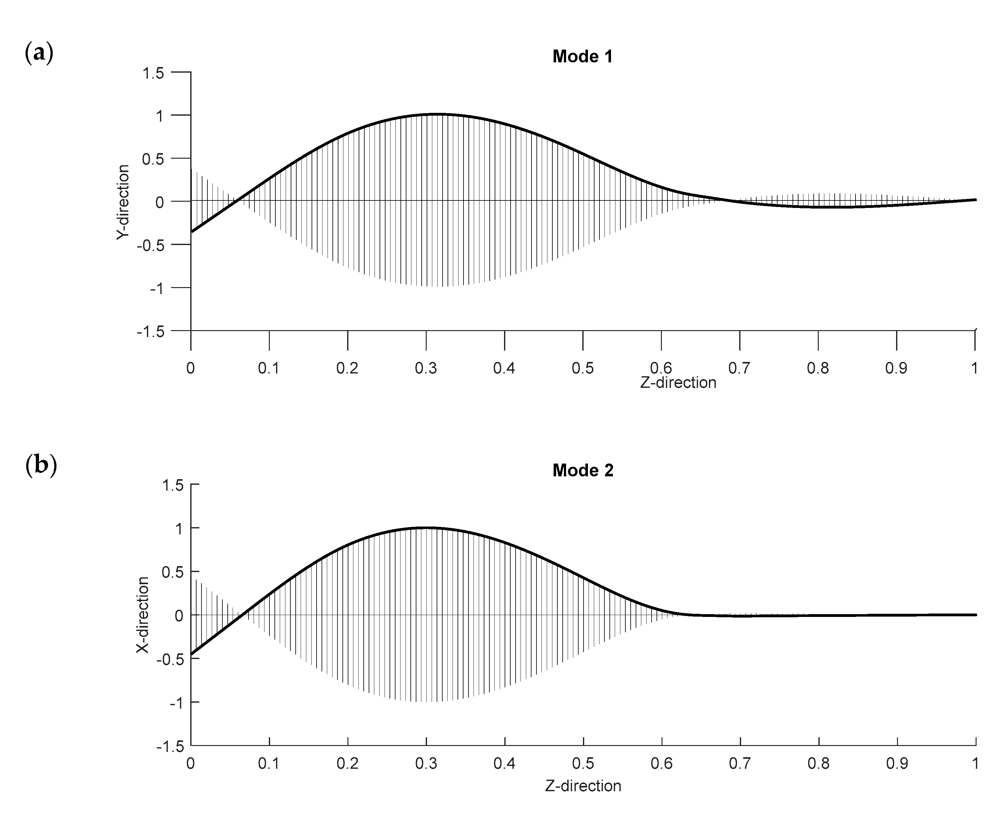
| Natural Frequency | Experimental, Hz | Mathematical, Hz | Error (%) | Dominant Direction |
|---|---|---|---|---|
| 50.6600 | 50.6650 | +0.010 | Y-direction | |
| 56.7600 | 56.7625 | +0.004 | X-direction |
| Actual | Healthy | Misalignment | Bow | Looseness | Rub | |
|---|---|---|---|---|---|---|
| Diagnosis | ||||||
| Healthy | 100.0 | 0.0 | 0.0 | 0.0 | 0.0 | |
| Misalignment | 0.0 | 100.0 | 0.0 | 0.0 | 0.0 | |
| Bow | 0.0 | 0.0 | 100.0 | 0.0 | 0.0 | |
| Looseness | 0.0 | 0.0 | 0.0 | 100.0 | 0.0 | |
| Rub | 0.0 | 0.0 | 0.0 | 0.0 | 100.0 | |
Publisher’s Note: MDPI stays neutral with regard to jurisdictional claims in published maps and institutional affiliations. |
© 2021 by the authors. Licensee MDPI, Basel, Switzerland. This article is an open access article distributed under the terms and conditions of the Creative Commons Attribution (CC BY) license (https://creativecommons.org/licenses/by/4.0/).
Share and Cite
Espinoza-Sepulveda, N.; Sinha, J. Mathematical Validation of Experimentally Optimised Parameters Used in a Vibration-Based Machine-Learning Model for Fault Diagnosis in Rotating Machines. Machines 2021, 9, 155. https://doi.org/10.3390/machines9080155
Espinoza-Sepulveda N, Sinha J. Mathematical Validation of Experimentally Optimised Parameters Used in a Vibration-Based Machine-Learning Model for Fault Diagnosis in Rotating Machines. Machines. 2021; 9(8):155. https://doi.org/10.3390/machines9080155
Chicago/Turabian StyleEspinoza-Sepulveda, Natalia, and Jyoti Sinha. 2021. "Mathematical Validation of Experimentally Optimised Parameters Used in a Vibration-Based Machine-Learning Model for Fault Diagnosis in Rotating Machines" Machines 9, no. 8: 155. https://doi.org/10.3390/machines9080155