Disturbance Detection of a Power Transmission System Based on the Enhanced Canonical Variate Analysis Method

Abstract

Aiming at the characteristics of dynamic correlation, periodic oscillation, and weak disturbance symptom of power transmission system data, this paper proposes an enhanced canonical variate analysis (CVA) method, called SLCVAkNN, for monitoring the disturbances of power transmission systems. In the proposed method, CVA is first used to extract the dynamic features by analyzing the data correlation and establish a statistical model with two monitoring statistics $T^2$ and Q. Then, in order to handling the periodic oscillation of power data, the two statistics are reconstructed in phase space, and the k-nearest neighbor (kNN) technique is applied to design the statistics nearest neighbor distance $D{T}^2$ and $DQ$ as the enhanced monitoring indices. Further considering the detection difficulty of weak disturbances with the insignificant symptoms, statistical local analysis (SLA) is integrated to construct the primary and improved residual vectors of the CVA dynamic features, which are capable to prompt the disturbance detection sensitivity. The verification results on the real industrial data show that the SLCVAkNN method can detect the occurrence of power system disturbance more effectively than the traditional data-driven monitoring methods.

1. Introduction

With the increasing demand on the power energy in the modern industry, power transmission systems are becoming more and more large-scale and complicated [1,2]. Due to the system complexity, anomalies and disturbances are often unavoidable in real power systems. If these unexpected events are not handled timely, they may cause huge accident risks and even the widespread power outages, which are companied by the huge economic loss and severe life inconvenience. Therefore, it is of great value to detect the abnormal events quickly and maintain the safe running of power systems [3]. In recent years, the wide area measurement system (WAMS) based on synchronous phaser technology has been successfully applied in the power industry. The phasor measurement units in WAMS provide the basic data support for the real-time dynamic monitoring of the power system [4]. Accordingly, safety monitoring and disturbance detection of power systems based on the measurement data analysis has been a hot topic in academic and engineering fields [5,6,7].

Aiming at the power system disturbance detection task, researchers have conducted a lot of studies, which can be roughly divided into two categories: time/frequency domain analysis and multivariate statistical analysis. The time/frequency domain analysis investigates the power system changes from the perspective of the signal processing, which involves the time domain, frequency domain, or time-frequency domain. In consideration of the good time-frequency localization property, Huang et al. [8] discussed the application of the Morelet wavelets method in power system disturbance detection. The Hilbert Huang Transform is another time-frequency signal analysis tool. Manglik et al. [9] applied it to the disturbance detection for the electric power system. Ghaderi et al. [10] proposed the time-frequency analysis method assisted by current waveform energy and normalized joint time-frequency moment and demonstrated its performance in the high-impedance ground fault detection. Salehi et al. [11] designed a morphological edge detection filter to obtain the transient features of fault signals. Liu et al. [12] used the wavelet packet Tsallis singularity entropy algorithm for disturbance detection. In general, the time/frequency domain analysis methods mainly analyze the single signal and fail to fully consider the correlation between different parameters. In response to this shortcoming, some scholars started their work by applying multivariate statistical analysis. Multivariate statistical analysis (MSA) methods can realize the simultaneous detection of multiple parameter changes and have outstanding advantages in the complex industrial systems. However, most of the present MSA studies focus on the system modeling and disturbance detection in the chemical process, steel industry, and high-train system [13,14,15,16,17], but MSA’s application to power system monitoring is very rare. Barocio et al. [18] first introduced the principal component analysis (PCA) method into the field of power system monitoring and discussed the detection and visualization of power system disturbances based on PCA. Guo et al. [19] built a transmission line fault detection method by combining PCA and support vector machine. Considering the masking influence caused by the oscillation trend and strong noise of power system data, Cai et al. [20] further proposed a PCAkNN method, which is superior to the basic PCA method in the numerical model testing and New England power system model data. These research articles point out that the multivariate statistical analysis has great application potential in the field of power system monitoring.

Although PCA and PCAkNN methods have achieved significant success in the power system monitoring field, they have some shortcomings deserving further studies. On the one hand, these methods do not take into account the dynamic characteristics of power system data, which easily leads to a high missing detection rate. Different from the other industrial process data with the steady operation mode, the power system data, such as the voltage and current, are with obvious dynamic trends. On the other hand, the present methods do not consider how to enhance the detection of weak disturbances. In real applications, some disturbances may be with small amplitudes, slow changes, unclear disturbance characteristics, and are easy to be covered by noises [21,22]. How to enhance the detection capability on these weak disturbances is one challenging task.

Aiming at the aforementioned problems, this paper proposes a SLCVAkNN-based disturbance detection method for power transmission system monitoring by combining canonical variate analysis (CVA), kNN, and statistical local analysis (SLA). Compared with the traditional PCA-based power system monitoring methods, CVA has a stronger dynamic feature extraction ability [23,24,25], which provides a new and powerful tool for power system data analysis. Referring to the present PCAkNN method, the CVAkNN statistical model is developed to deal with the dynamic periodic oscillation signals. Furthermore, in order to enhance the detection of weak faults, SLA is integrated for SLCVAkNN modeling, which mines the local statistical information for better weak disturbance monitoring.

The rest of the paper’s content is arranged as follows. The principle of the proposed SLCVAkNN methodology is given in the Section 2, while the corresponding disturbance detection procedure is detailed in Section 3. One case study on the actual industrial data is used to verify the effectiveness of the proposed method.

2. The Proposed Methodology

This section clarifies the proposed SLCVAkNN-based power system disturbance detection method. The whole methodology involves three parts: dynamic system modeling using canonical variate analysis, monitoring index construction based on kNN, and weak disturbance detection by statistical local analysis.

2.1. CVA Monitoring Model

A power system is a classical dynamic process [26,27], where the measurement data demonstrate the clear trend along the sampling time. The measured three-phase electric field and current waveform change with time, and the current data point has a certain correlation with the historical samples. Therefore, it is more reasonable to apply the dynamic data analysis tool to extract the process features.

Canonical variate analysis (CVA) is an effective dynamic data analysis tool, which has been applied to the model identification and control in the multivariate dynamic system [28,29]. This paper introduces it to deal with power system data. For a certain power transmission line, the data points under normal system operation have a fixed correlation along the time dimension. When a disturbance occurs, this correlation may be destroyed. By monitoring the correlation among the time series data, CVA can find the system disturbance effectively. When CVA is applied to data modeling, the training data are firstly divided into the historical data set and the future data set, and the CVA optimization problem is designed to find the maximum correlation between these two data sets for describing the data dynamic features. The algorithm details are clarified as follows.

For the power system measurement data vector ${\mathit{x}}_h\in {\mathit{R}}^m$ at the h-th sampling instant, its corresponding historical data vector ${\mathit{p}}_h$ and future data vector ${\mathit{f}}_h$ are constructed as

$${\mathit{p}}_h={[{\mathit{x}}_h^T,{\mathit{x}}_{h-1}^T,\cdots ,{\mathit{x}}_{h-l+1}^T]}^T\in {\mathit{R}}^M$$

(1)

$${\mathit{f}}_h={[{\mathit{x}}_{h+1}^T,{\mathit{x}}_{h+2}^T,\cdots ,{\mathit{x}}_{h+l}^T]}^T\in {\mathit{R}}^M$$

(2)

where $M=m\times l$, and l represents the time lag order.

Given the projection vectors $\mathit{a}$ and $\mathit{b}$, they are used to transform the historical and future vectors into their respective projections $d={\mathit{a}}^T{\mathit{p}}_h$ and $v={\mathit{b}}^T{\mathit{f}}_h$. CVA is to optimize the vector pair $\mathit{a}$ and $\mathit{b}$ so that the correlation between d and v is maximized, which are also called canonical variates. This can be described by the mathematical expression as

$$\left\{\begin{array}{cc}\hfill & \underset{\mathit{a},\mathit{b}}{max}\rho (d,v)={\mathit{a}}^T{\mathsf{\Sigma }}_{pf}\mathit{b}\hfill \\ \hfill \mathrm{s}.\mathrm{t}.& var\left(d\right)={\mathit{a}}^T{\mathsf{\Sigma }}_{pp}\mathit{a}=1\hfill \\ \hfill & var\left(v\right)={\mathit{b}}^T{\mathsf{\Sigma }}_{ff}\mathit{b}=1\hfill \end{array}\right.$$

(3)

where ${\mathsf{\Sigma }}_{pf}$ represents the cross-covariance matrix of the historical and future data vectors, and ${\mathsf{\Sigma }}_{pp},{\mathsf{\Sigma }}_{ff}$ denote the covariance matrix of the historical and future data vectors, respectively.

Suppose that the training data set includes n samples as $\mathit{X}={[{\mathit{x}}_1^T,{\mathit{x}}_2^T,\cdots ,{\mathit{x}}_n^T]}^T\in R^{n\times m}$, then the historical and future data matrix can be expressed by

$$\mathit{P}={[{\mathit{p}}_l^T,{\mathit{p}}_{l+1}^T,\cdots ,{\mathit{p}}_{n-l}^T]}^T\in {\mathit{R}}^{N\times M}$$

(4)

$$\mathit{F}={[{\mathit{f}}_l^T,{\mathit{f}}_{l+1}^T,\cdots ,{\mathit{f}}_{n-l}^T]}^T\in {\mathit{R}}^{N\times M}$$

(5)

where $N=n-2l+1$ is the sample number of the historical and future data matrix. Then the covariance matrices defined in Equation (3) can be calculated by

$${\mathsf{\Sigma }}_{pf}=\frac{1}{N-1}{\mathit{P}}^T\mathit{F}$$

(6)

$${\mathsf{\Sigma }}_{pp}=\frac{1}{N-1}{\mathit{P}}^T\mathit{P}$$

(7)

$${\mathsf{\Sigma }}_{ff}=\frac{1}{N-1}{\mathit{F}}^T\mathit{F}$$

(8)

Solving the optimization problem described by Equation (3) leads to a singular value decomposition on the matrix $\mathsf{\Xi }={\mathsf{\Sigma }}_{pp}^{-1/2}{\mathsf{\Sigma }}_{pf}{\mathsf{\Sigma }}_{ff}^{-1/2}$, which is expressed by

$$\mathsf{\Xi }={\mathit{U}\mathsf{\Lambda }\mathit{V}}^T$$

(9)

The solution of Equation (9) is further used to build the a series of the projection vectors ${\mathit{a}}_i$ and ${\mathit{b}}_i(1\le i\le M)$, which are computed by

$${\mathit{a}}_i={\mathsf{\Sigma }}_{pp}^{-1/2}\mathit{U}(:,i),{\mathit{b}}_i={\mathsf{\Sigma }}_{ff}^{-1/2}\mathit{V}(:,i),$$

(10)

where $(:,i)$ represents the i-th column of the matrix. The vectors ${\mathit{a}}_i$ and ${\mathit{b}}_i$ are ordered by the corresponding correlation degree, which is given in the diagonal elements of matrix $\mathsf{\Lambda }$, also meaning the correlation coefficients. The first s pairs of projection vectors $\{{\mathit{a}}_i,{\mathit{b}}_i,1\le i\le s\}$ describe the stronger correlation and indicate the close relationship between the historical data and the future data. Therefore, a projection matrix ${\mathit{A}}_s=[{\mathit{a}}_1{\mathit{a}}_2\cdots {\mathit{a}}_s]$ is defined to extract the canonical variate vector ${\mathit{d}}_h$ as

$${\mathit{d}}_h={\mathit{A}}_s^T{\mathit{p}}_h.$$

(11)

which describes the main dynamic features of process data. Here, s is determined so that the corresponding canonical variate vectors describe a cumulative percentage of 90% of correlation coefficients.

As ${\mathit{A}}_s$ only involves the first s projection directions, it cannot cover all the data information. The rest information in the CVA model can be described by the CVA residual vector ${\mathit{e}}_h$ as

$${\mathit{e}}_h=(\mathit{I}-{\mathit{A}}_s{\mathit{A}}_s^T){\mathit{p}}_h$$

(12)

Based on the canonical variate vector and CVA residual vector, two monitoring statistics $T^2$ and Q are often used to judge the process state. The $T^2$ statistic describes the changes of principal dynamic states, while the Q statistic monitors the changes of the residual information. For the h-th sample, the statistics are written by

$$T_h^2={\mathit{d}}_h^T{\mathit{d}}_h$$

(13)

$$Q_h={\mathit{e}}_h^T{\mathit{e}}_h$$

(14)

In the normal operation, these two statistics should satisfy $T_h^2\le T_{h,lim}^2$ and $Q_h\le Q_{h,lim}$, where $T_{h,lim}^2$ and $Q_{h,lim}$ are the corresponding confidence limits. In some literature, the confidence limits of these two statistics can be obtained by assuming the prior distribution [30]. However, these distribution assumptions are often difficult to satisfy. Therefore, this paper applies the data-driven kernel density estimation to determine the confidence limit [31,32].

2.2. CVAkNN Model Based on kNN Monitoring Index

As the measurement data of power transmission systems have the periodic fluctuation characteristic, the traditional CVA monitoring statistics $T^2$ and Q behave unsteadily with the periodic changes. In this case, disturbance detection by directly monitoring the amplitudes of monitoring statistics cannot discover the disturbance signals effectively and may lead to a high disturbance missing rate.

In order to overcome this defect, this paper introduces the k-nearest neighbor analysis (kNN) to enhance the basic monitoring statistics. kNN is one effective multimodal data analysis tool and does not depend on the amplitude changes before and after the disturbance. In the literature [33,34], kNN was introduced and adapted for real-time detection of system disturbances. By combining the CVA model and the kNN-based monitoring statistics, the improved method, which is called CVAkNN, has a stronger capability of dealing with the periodic oscillation data property. The main idea of CVAkNN is to first reconstruct the monitoring statistic in the phase space and then build the monitoring index based on the distance between the reconstructed statistic vector and its k-nearest neighbor.

Phase space reconstruction is a good method to deal with time series analysis. This method regards one-dimensional time series as the result of nonlinear dynamic system motion and constructs the phase vectors by re-arranging the time series. This theory has been successfully applied in the fields of chaotic time series prediction and equipment failure data analysis [35,36]. Here it is introduced to deal with the CVA monitoring statistics for the further kNN analysis.

For the training data set with n samples ${\mathit{x}}_1,{\mathit{x}}_2,\dots ,{\mathit{x}}_n$, the corresponding statistics vectors are obtained by the CVA modeling as

$${\mathit{T}}^2=[T_l^2{T}_{l+1}^2\cdots T_n^2]$$

(15)

$$\mathit{Q}=[Q_l{Q}_{l+1}\cdots Q_n]$$

(16)

Further, the phase reconstruction statistics matrix can be formulated as follows:

$$\begin{array}{c}\hfill {\mathit{MT}}^2=\left[\begin{array}{cccc}{T}_l^2& \cdots & T_{l+L-2}^2& T_{l+L-1}^2\\ T_{l+1}^2& \cdots & T_{l+L-1}^2& T_{l+L}^2\\ ⋮& ⋮& ⋮& ⋮\\ T_{n-L+1}^2& \cdots & T_{n-1}^2& T_n^2\end{array}\right]\end{array}$$

(17)

$$\begin{array}{c}\hfill \mathit{MQ}=\left[\begin{array}{cccc}{Q}_l& \cdots & Q_{l+L-2}& Q_{l+L-1}\\ Q_{l+1}& \cdots & Q_{l+L-1}& Q_{l+L}\\ ⋮& ⋮& ⋮& ⋮\\ Q_{n-L+1}& \cdots & Q_{n-1}& Q_n\end{array}\right]\end{array}$$

(18)

where L is the embedding dimension defining the length of the reconstructed phase vector. Based on the results of the phase space reconstruction, the dynamic behavior of the statistics can be better described, which is conducive to the detection of power system disturbances.

In the online monitoring stage, a new testing sample ${\mathit{x}}_t$ is collected at the t-th sampling instant. Then the monitoring statistics can be computed by applying Equations (13) and (14), and the reconstructed phase vectors are described as

$$\begin{array}{c}\hfill {\mathit{NT}}_t^2=\left[T_{t-L+1}^2\cdots T_{t-1}^2{T}_t^2\right]\end{array}$$

(19)

$$\begin{array}{c}\hfill {\mathit{NQ}}_t=\left[Q_{t-L+1}\cdots Q_{t-1}{Q}_t\right]\end{array}$$

(20)

To determine whether the test data ${\mathit{x}}_t$ is normal, it is necessary to compare the similarity between ${\mathit{NT}}_t^2,{\mathit{NQ}}_t^2$, and the reconstructed statistics matrix in Equations (17) and (18). If the reconstructed statistics ${\mathit{NT}}_t^2,{\mathit{NQ}}_t^2$ are strongly similar to one column of the training statistics vectors in Equations (17) and (18), then the test data $x_t$ describe the normal working condition. Otherwise, it means that some faults occur in the power transmission system. Therefore, the key is how to perform this similarity comparison. This paper introduces the k-nearest neighbor (kNN) analysis to construct a kNN-based distance measurement indicator: statistical nearest neighbor distance (SNND).

The idea of SNND is to find the first k-th nearest neighbors of the test vector in the given matrix data and compute the distance between the test vector and the k-th nearest neighbors as a disturbance detection criterion. The SNND index for ${\mathit{NT}}_t^2$ is defined as

$$\begin{array}{c}\hfill D{T}_t^2=\left|\left|{\mathit{NT}}_t^2-{\mathit{MT}}^2\left(j_k,:\right)\right|\right|,\end{array}$$

(21)

where ${\mathit{MT}}^2(j_k,:)$ represents the $j_k$-th row in the ${\mathit{MT}}^2$ matrix, which corresponds to the k-th nearest neighbor of ${\mathit{NT}}_t^2$, and $\left|\left|.\right|\right|$ represents the L2 norm calculation. By analogy, the SNND indicator of $N{Q}_t$ can be established as

$$\begin{array}{c}\hfill D{Q}_t=\left|\left|{\mathit{NQ}}_t-\mathit{MQ}\left(j_k,:\right)\right|\right|.\end{array}$$

(22)

Under normal operating conditions, the above two indicators should fluctuate within a relatively small range. That means $D{T}_t^2\le D{T}_{lim}^2$ and $D{Q}_t\le D{Q}_{lim}$ for the normal running status. Once the threshold is exceeded, it means that there is a system disturbance. The threshold can be obtained by the kernel density estimation method.

2.3. SLCVAkNN Model Assisted by Statistical Local Analysis

In the power transmission system, some weak disturbances are often difficult to detect, such as the high-impendence single-phase ground fault. When this kind of disturbance occurs, the changes reflected by the measure voltage and current variables are very small. Further, considering the influence of modeling error and process noise, this kind of disturbance may be concealed and viewed as the normal process changes. Therefore, enhacning the weak disturbance detection is of great value to ensure the safety of power transmission systems. In this paper, we integrate the statistical local analysis (SLA) with CVAkNN and propose an improved SLCVAkNN monitoring model for better weak disturbance monitoring performance.

SLA was originally proposed by Basseville [37] for inspecting the process parameter changes. In recent years, some researchers have introduced it into the chemical process fault detection and demonstrated its effectiveness [38,39,40]. In this paper, we will perform the statistical local analysis on the CVA model. To look back into the CVA monitoring statistics in Equations (13) and (14), it is found that the monitoring statistics used to indicate the process status are composed of the canonical variate vector ${\mathit{d}}_h$ and the CVA residual vector ${\mathit{e}}_h$. Therefore, if we attempt to improve the weak disturbance monitoring of CVA statistics, the vectors ${\mathit{d}}_h$ and ${\mathit{e}}_h$ must be improved with stronger disturbance sensitivity.

According to the statistical local analysis theory, given the system observation ${\mathit{z}}_j$ and the system parameter $\mathit{\vartheta }$, a primary residual vector $\phi ({\mathit{z}}_j,\mathit{\vartheta })$ can be defined for disturbance detection if it meets the following conditions: [37,38]

• $E\left\{\phi ({\mathit{z}}_j,\mathit{\vartheta })\right\}=0$, if $\mathit{\vartheta }={\mathit{\vartheta }}_0$;
• $E\left\{\phi ({\mathit{z}}_j,\mathit{\vartheta })\right\}\ne 0$, if $\mathit{\vartheta }$ is in the neighborhood of ${\vartheta }_0$, but $\mathit{\vartheta }\ne {\mathit{\vartheta }}_0$;
• $\phi ({\mathit{z}}_j,\mathit{\vartheta })$ is differentiable with $\mathit{\vartheta }$;
• $\phi ({\mathit{z}}_j,\mathit{\vartheta })$ exists for $\mathit{\vartheta }$ in the neighborhood of ${\mathit{\vartheta }}_0$.

Here ${\mathit{\vartheta }}_0$ represents the parameters under the normal condition.

By investigating the i-th element in the vector ${\mathit{d}}_h$, which is denoted as $d_{h,i}$, it is easily derived by Equation (11) that $d_{h,i}={\mathit{a}}_i^T{\mathit{p}}_h$. Naturally, the variance of $d_{h,i}$ can be computed as

$$E\left\{d_{h,i}^2\right\}={\mathit{a}}_i^{T}E\left\{{\mathit{p}}_h{\mathit{p}}_h^T\right\}{\mathit{a}}_i$$

(23)

For the statistical samples, $E\left\{{\mathit{p}}_h{\mathit{p}}_h^T\right\}$ is factually equal to the covariance matrix ${\mathsf{\Sigma }}_{pp}$. Further combining the first constraint on the vector $\mathit{a}$ in Equation (3), it is known that ${\mathit{a}}_i^{T}E\left\{{\mathit{p}}_h{\mathit{p}}_h^T\right\}{\mathit{a}}_i=1$. Therefore, we build the SLA primary residual of the canonical variate as

$${\phi }_{d_{h,i}}=d_{h,i}^2-1.$$

(24)

which meets the condition $E\left\{{\phi }_{d_{h,i}}\right\}=0$ in the normal condition.

Similarly, we analyze the variance of $e_{h,i}$ to obtain

$$E\left\{e_{h,i}^2\right\}={\mathit{A}}_r(i,:)E\left\{{\mathit{p}}_h{\mathit{p}}_h^T\right\}{\mathit{A}}_r{(i,:)}^T$$

(25)

As ${\mathit{A}}_r$ can be obtained in the model training procedure, the above expression must be equal to a fixed value, which is denoted as ${\sigma }_i={\mathit{A}}_r(i,:)E\left\{{\mathit{p}}_h{\mathit{p}}_h^T\right\}{\mathit{A}}_r{(i,:)}^T$. Therefore, the SLA primary residual of the CVA residual can be built as

$${\phi }_{e_{h,i}}=e_{h,i}^2-{\sigma }_i.$$

(26)

which meets the condition $E\left\{{\phi }_{e_{h,i}}\right\}=0$ for the normal data.

For a more sensitive disturbance detection, the SLA improved residual is applied in a moving window with the width of w, which is expressed by

$$\begin{array}{c}\hfill {\psi }_{d_{h,i}}=\left\{\begin{array}{c}\frac{1}{\sqrt{h}}{\displaystyle \sum _{j=1}^h}{\phi }_{d-j,i},h<w\\ \frac{1}{\sqrt{w}}{\displaystyle \sum _{j=h-w+1}^h}{\phi }_{d_{j,i}},h\ge w\end{array}\right.\end{array}$$

(27)

$$\begin{array}{c}\hfill {\psi }_{e_{h,i}}=\left\{\begin{array}{c}\frac{1}{\sqrt{h}}{\displaystyle \sum _{j=1}^h}{\phi }_{e_{j,i}},h<w\\ \frac{1}{\sqrt{w}}{\displaystyle \sum _{j=h-w+1}^h}{\phi }_{e_{j,i}},h\ge w\end{array}\right.\end{array}$$

(28)

Up to now, we can obtain the SLA improved residual vectors ${\mathit{\psi }}_{d,h}={[{\psi }_{d_{h,1}}{\psi }_{d_{h,2}}\cdots {\psi }_{d_{h,s}}]}^T$ and ${\mathit{\psi }}_{e,h}={[{\psi }_{e_{h,1}}{\psi }_{e_{h,2}}\cdots {\psi }_{e_{h,M}}]}^T$. These residual vectors are used to replace the original CVA features ${\mathit{d}}_h$ and ${\mathit{e}}_h$ so that the monitoring model is modified to the SLCVAkNN model.

With the SLA improved residual vectors, the monitoring statistics are constructed as follows:

$$T_h^2={\mathit{\psi }}_{d,h}^T{\mathit{\psi }}_{d,h}$$

(29)

$$Q_h={\mathit{\psi }}_{e,h}^T{\mathit{\psi }}_{e,h}$$

(30)

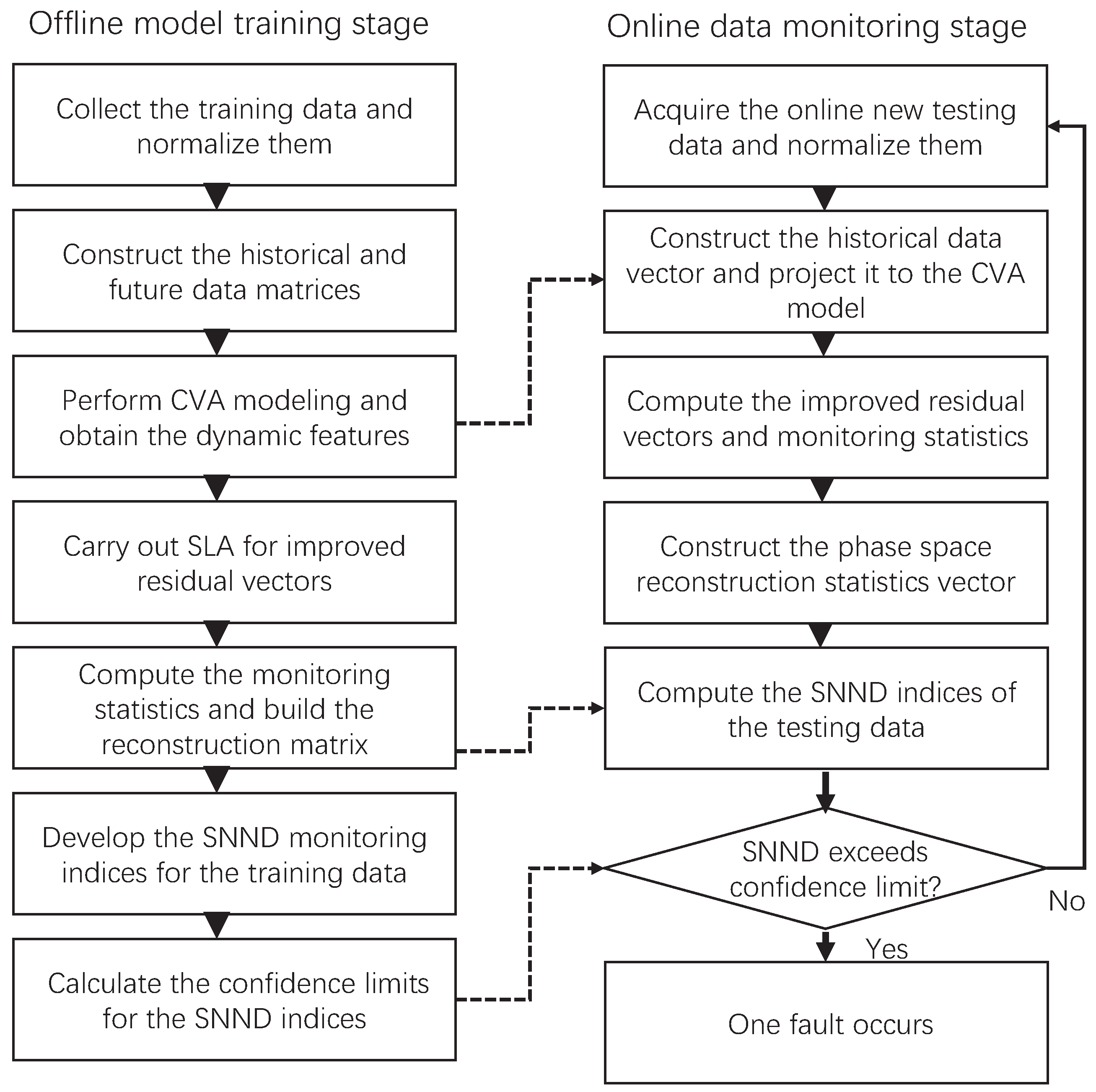
3. Disturbance Detection Procedure Based on SLCVAkNN

Power transmission system disturbance detection based on SLCVAkNN method is divided into two stages: offline modeling stage and online detection stage. The corresponding flowchart is shown in Figure 1.

• Stage 1: offline modeling stage
  • Acquire the normal condition data to constitute the training data set $\mathit{X}={[{\mathit{x}}_1^T,{\mathit{x}}_2^T,\cdots ,{\mathit{x}}_n^T]}^T\in R^{n\times m}$ and perform data normalization processing. Here, the mentioned normal condition data mean the data from a section of transmission line between two adjacent nodes. For different lines, the corresponding modelings are needed separately.
  • Construct historical data sets $\mathit{P}$ and future data sets $\mathit{F}$ according to Equations (4) and (5), calculate the covariance matrices by Equations (6)–(8), and solve the CVA optimization by the SVD as Equation (9).
  • Extract the canonical variate vector ${\mathit{d}}_h$ and the CVA residual vector ${\mathit{e}}_h$, as shown in Equations (11) and (12).
  • Perform Equations (24) and (26) to obtain the SLA primary residual vectors and further calculate the SLA improved residual vectors by Equations (27) and (28).
  • Compute the monitoring statistics $T_h^2$ and $Q_h$ for all the training samples according to Equations (29) and (30).
  • Construct the statistics matrix in the phase space according to Equations (17) and (18).
  • Calculate the SNND monitoring indices $D{T}^2$ and $DQ$ for all the training samples and determine the 95% confidence limits $D{T}_{lim}^2$ and $D{Q}_{lim}$ by kernel density estimation.
• Stage 2: online detection stage
  • Obtain online new data ${\mathit{x}}_t$ and normalize it with the training data.
  • Construct the corresponding historical vector ${\mathit{p}}_t$ and project the ${\mathit{p}}_t$ to the CVA model and obtain the canonical variate vector ${\mathit{d}}_t$ and ${\mathit{e}}_t$ according to Equations (11) and (12).
  • Apply Equations (24), (26)–(28) to compute the SLA primary residual vector and the improved residual vector orderly.
  • Compute the monitoring statistics $T_t^2$ and $Q_t$ for the online new sample ${\mathit{x}}_t$ according to Equations (29) and (30).
  • Construct the phase space statistics vector ${\mathit{NT}}_t^2$ and ${\mathit{NQ}}_t^2$, and calculate the SNND index $D{T}_t^2$ and $D{Q}_t^2$ by Equations (21) and (22).
  • Compare the SNND indices with the corresponding confidence limits $D{T}_{lim}^2$ and $D{Q}_{lim}$. If any one exceeds the confidence limit, a disturbance sample is indicated.

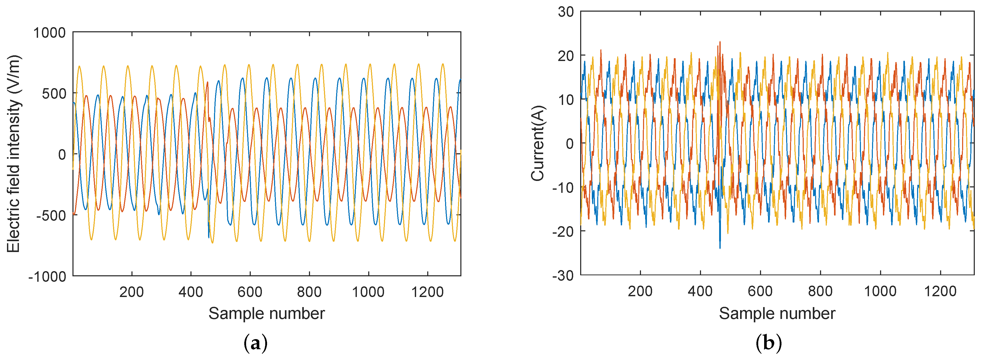
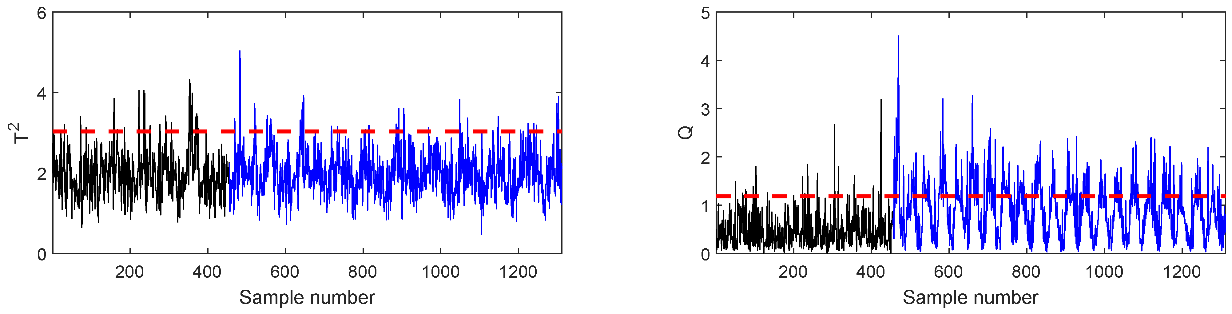
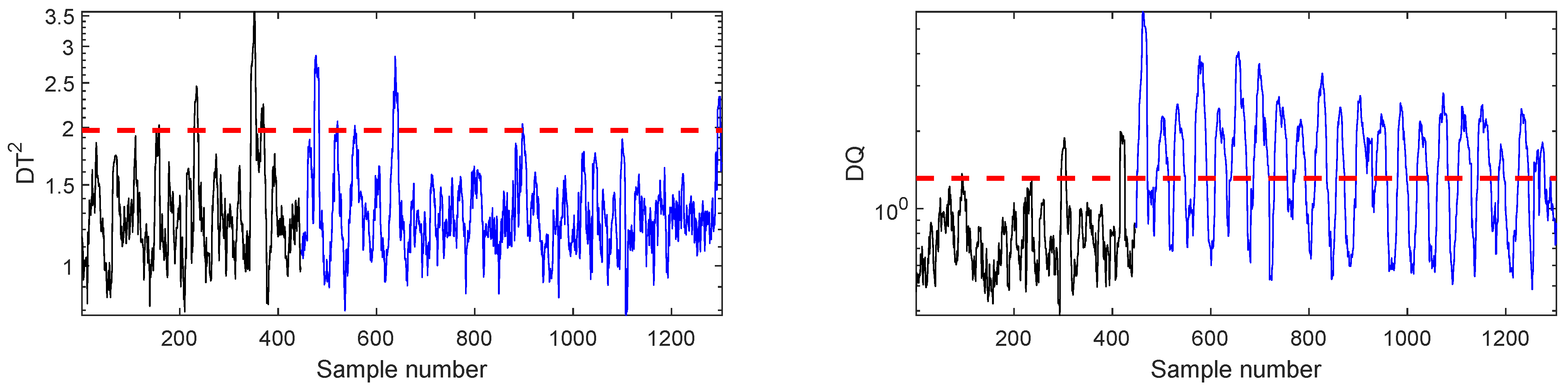
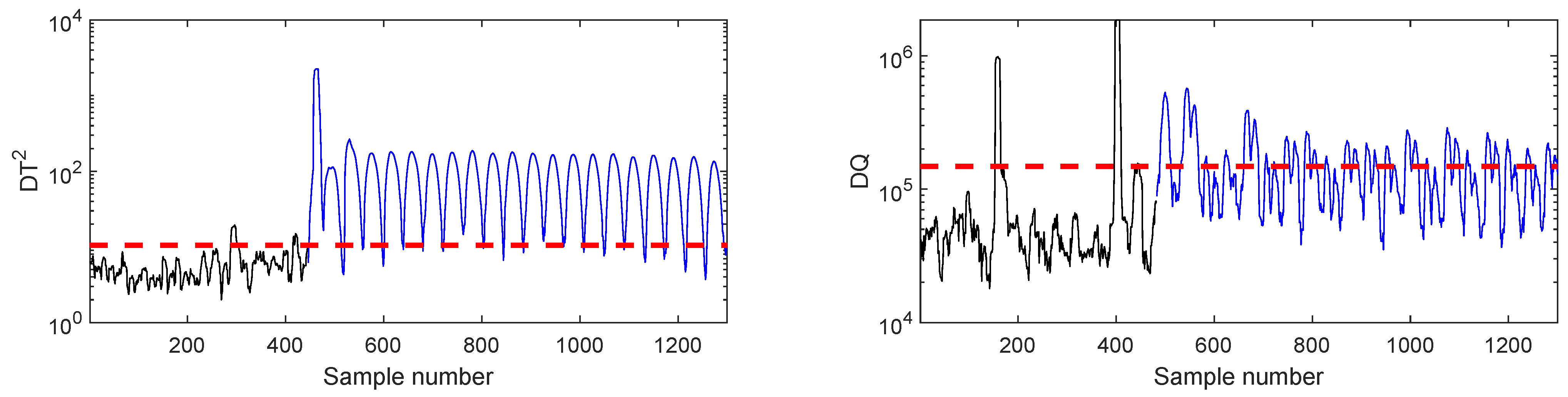
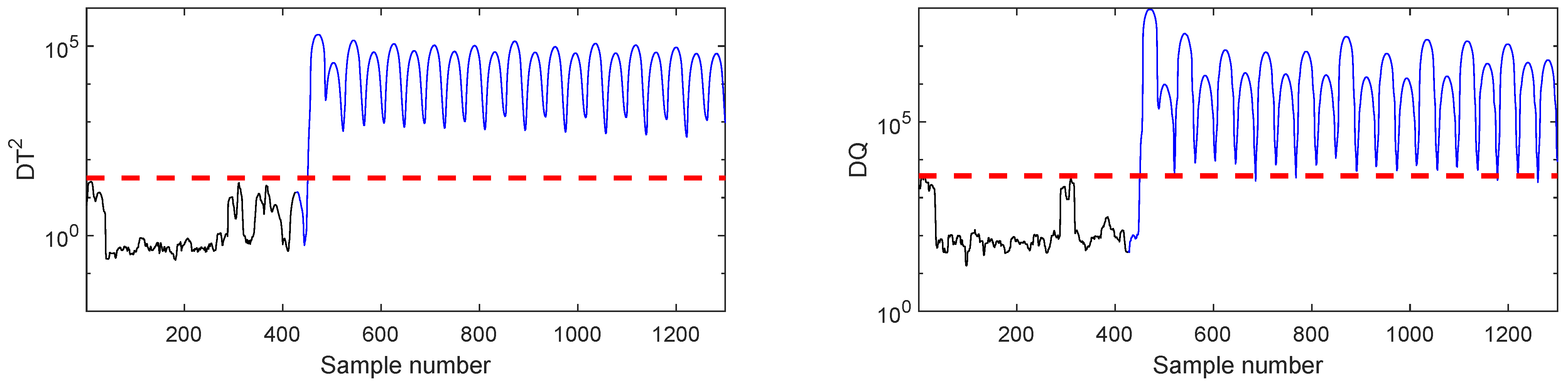
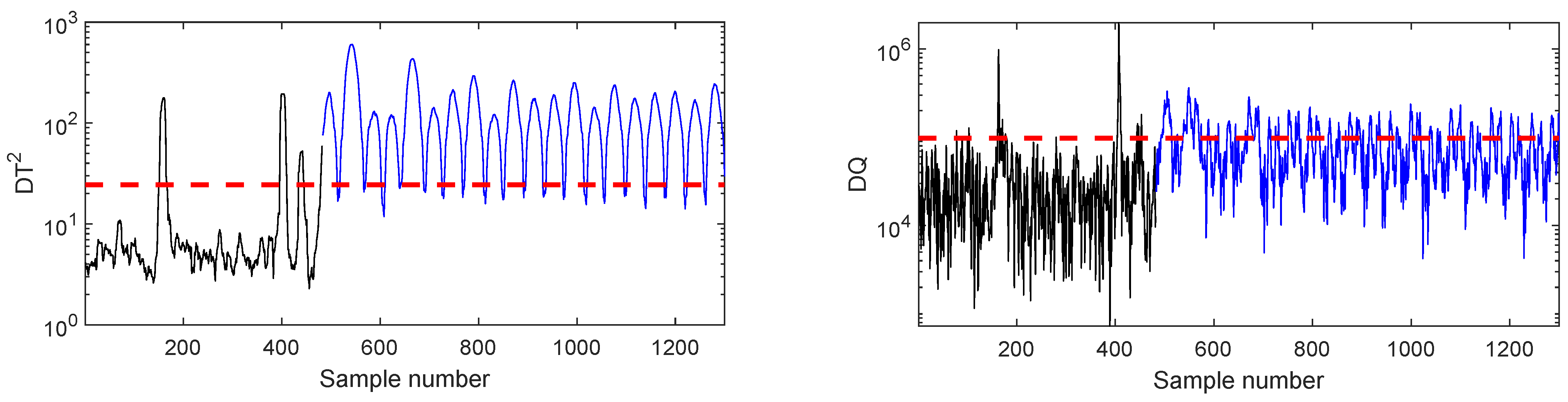
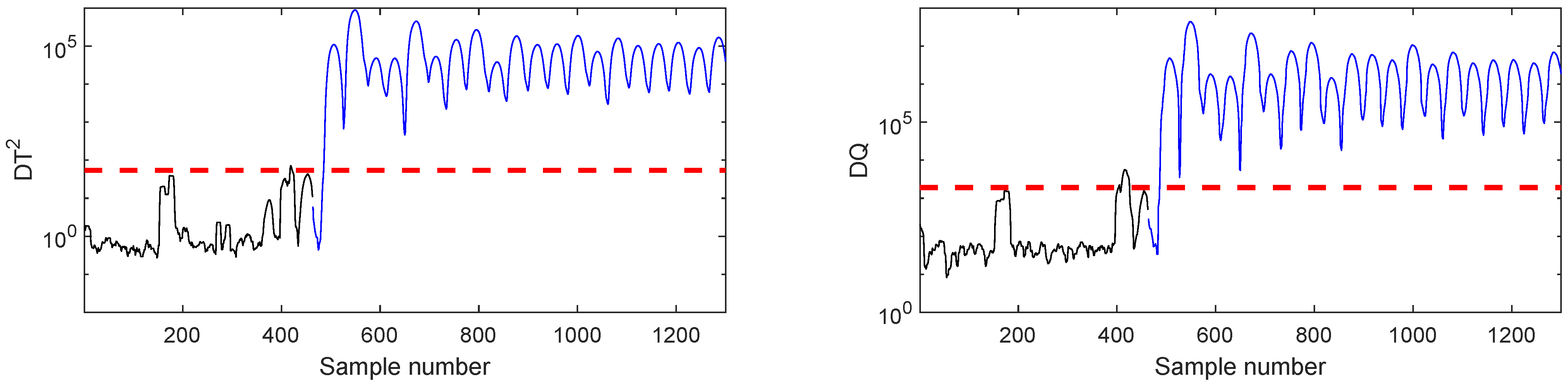
Here, it is pointed out that the local neighborhood standardization (LNS) [41] may be used to enhance the traditional z-score standardization. Compared with the traditional z-score method, LNS has better capability to deal with the non-steady data with the periodic oscillations.

4. Case Analysis

In order to verify the advantages of the SLCVAkNN method in the power transmission system disturbance detection, this section gives the case study on the real industrial data collected from the actual power transmission system. For method comparison, four methods, including the proposed SLCVAkNN method and three other methods of PCA, PCAkNN, and CVAkNN, are all applied to build the monitoring models for disturbance detection. The PCA method has two monitoring statistics $T^2$ and Q, while the other three methods are with the kNN-based statistics $D{T}^2$ and $DQ$. When these methods are used, they indicate the system status by the monitoring charts, where the monitoring indices of normal and faulty samples are given by black and blue solid lines, respectively, while the detection threshold, that is the 95% confidence limit of the monitoring index, is plotted by the red dashed line. One evaluation index, called the disturbance detection rate (DDR), is used to evaluate the different monitoring methods. DDR is the percentage of the abnormal samples exceeding the detection threshold over all the abnormal samples.

The used real industrial data are collected from the seven transmission lines in a power supply station in August 2018. These lines are radially connected. Their data are collected because all of them involve the ground fault. The data acquisition units, designed by Qingdao Topscomm Communication CO. LTD, are used to collect the electric field intensity and current. Here, the real line voltage is up to 110 KV so that the existing equipment can not directly measure it. Therefore, the electric field intensity is applied to reflect the voltage trend. For each transmission line, one corresponding data set is recorded that involves the normal state and the abnormal state. The data set has the length of about 1300 samples, where the disturbance starting time (DST) is different in different transmission lines. The detailed information about the acquired data sets are listed in

Table 1. The collected industrial data sets.

No.	Description	DST
DATA-1	Data set collected from line 904 exit	446
DATA-2	Data set collected from line 906, pole 116-3	456
DATA-3	Data set collected from line 906, pole 90-2	445
DATA-4	Data set collected from line 906, pole 151-5	458
DATA-5	Data set collected from line 906, pole 97-1	452
DATA-6	Data set collected from line 906 exit	493
DATA-7	Data set collected from line 907 exit	420

, where DST data record the sample number corresponding to the disturbance starting time. A demonstration of the collected data for the DATA-A is given in Figure 2, where six measured variables, including the electric field intensities of phase A, B, and C, and the currents of phase A, B, and C, are involved. Due to the existence of the harmonic load, the current sine wave distortion can be seen in these curves.

Taking the data set DATA-2 as one example, it is collected from the pole 116-3 of the line 906. This data set includes 1312 samples. To investigate it with the help of on-site engineers, it is known that the disturbance occurs from the 456th sample. Although engineers can find this disturbance by careful analysis, this manual way is very time-consuming and inefficient, so it is difficult to implement in large-scale transmission system monitoring. Therefore, building an automatic multivariate data analysis tool is very necessary. In this section, we apply four MSA methods, which are PCA, PCAkNN, CVAkNN, and SLCVAkNN, to perform the automatic fault detection. When the statistical models are developed, the model parameters are set as follows: $k=3,L=10,l=2,w=20$. For the data set DATA-2, the first 320 sampling point are considered to be in a normal operating state, they can be utilized as the training data set for model development, while monitoring charts of PCA, PCAkNN, CVAkNN, and SLCVAkNN are demonstrated in the Figure 3, Figure 4, Figure 5 and Figure 6, respectively. By the PCA monitoring results shown in Figure 3, it can be seen that the disturbance cannot be detected very effectively. The DDR of PCA $T^2$ is 4.43%, while the Q is a little better with the DDR of 29.52%. When PCAkNN is used, the $D{T}^2$ has a similarly poor detection rate, but the $DQ$ statistic achieves clear improvement with the DDR of 57.76%. These results demonstrate that the PCAkNN method proposed by Cai et al. [20] can deal with the power system data with oscillation characteristic effectively. However, from these figures, the monitoring statistics do not exceed the confidence limits significantly. This may lead to the uncertain judgement on the occurrence of disturbance. When the CVAkNN is applied in Figure 5, the $DQ$ statistic performs a little better with the DDR of 49.71%. However, its $D{T}^2$ indicator clearly improves the DDR to 92.51%, which means a significant detection rate improvement of about 70% in contrast with the PCAkNN’s $DQ$ index. The best monitoring results on this data set is provided by SLCVAkNN, which are shown in Figure 6. By this figure, it is observed that the disturbance is detected very clearly with the DDRs of 97.25% and 96.80% for $D{T}^2$ and $DQ$, respectively. This case gives a comprehensive comparison on the four methods of PCA, PCAkNN, CVAkNN, and SLCVAkNN. The applications show that PCAkNN does better than PCA due to the use of kNN, while SLCVAkNN further prompts the disturbance detection performance with the integration of CVA and SLA.

Another example on the data set DATA-6 is illustrated, which corresponds to the line 906 exit. The modeling procedure is similar to the above case. Here we only give the monitoring charts of CVAkNN and SLCVAkNN, as shown in the Figure 7 and Figure 8. With the consideration of system dynamics, the CVAkNN $D{T}^2$ monitoring chart gives a higher DDR of 88.51%. Compared with the CVAkNN method, which has only one effective monitoring statistic, SLCVAkNN has two well-behaved monitoring statistics. The $D{T}^2$ and $DQ$ have the DDRs of 97.37% and 97.25%, respectively. The testing results on DATA-6 further verify the advantage of the proposed method over the CVAkNN method.

The summary of disturbance detection rates for all seven data sets are shown in

Table 2. The disturbance detection rate of PCA, PCAkNN, CVAkNN, and SLCVAkNN for the tested data sets.

NO.	PCA		PCAkNN		CVAkNN		SLCVAkNN
	${\mathit{T}}^{\mathbf{2}}$	$\mathit{Q}$	${\mathit{DT}}^{\mathbf{2}}$	$\mathit{DQ}$	${\mathit{DT}}^{\mathbf{2}}$	$\mathit{DQ}$	${\mathit{DT}}^{\mathbf{2}}$	$\mathit{DQ}$
DATA-1	7.50%	70.47%	26.18%	90.89%	96.76%	64.39%	96.83%	89.48%
DATA-2	4.43%	29.52%	3.85%	57.76%	92.51%	49.71%	97.25%	96.80%
DATA-3	5.99%	83.06%	19.93%	97.81%	100.00%	100.00%	97.85%	97.97%
DATA-4	5.15%	10.18%	8.54%	26.78%	96.60%	51.93%	97.36%	96.79%
DATA-5	48.78%	96.05%	82.81%	99.54%	100.00%	100.00%	98.06%	98.29%
DATA-6	4.39%	77.44%	5.49%	92.20%	88.51%	41.20%	97.37%	97.25%
DATA-7	7.95%	84.99%	11.09%	95.97%	93.49%	55.33%	97.47%	97.47%
Average	12.03%	64.53%	22.56%	80.13%	95.41%	66.08%	97.46%	96.29%

. From this table, it is shown that the faults in DATA-2 and DATA-4 are difficult to detect by PCA, whose DDRs are all lower than 30%. By the use of PCAkNN, these two faults are detected with higher DDRs, which are 57.76% and 26.78%, respectively. By contrast, CVAkNN does better on the two faults. In particular, its $D{T}^2$ statistic gives the DDR higher than 90%. When SLCVAkNN is used, its two monitoring statistics have the higher DDRs than 95%. For the sets of DATA-1, DATA-3, DATA-6, and DATA-7, PCA can detect these faults with about 70-80% DDR on one statistic. That means PCA can alarm these faults, but the alarm degree is not very sufficient. The PCAkNN and CVAkNN improve the DDR to about 90%. Further combining the SLA technique, SLCVAkNN achieves higher DDR than CVAkNN on these four sets. As to DATA-5, all these four methods give a similarly good performance with the DDRs higher than 95%. Considering all seven of these data sets, we observe that the average detection rates of CVAkNN outperforms the PCA and PCAkNN method, while the ones of SLCVAkNN statistics can reach 97.46% and 96.29%, which are the highest among these four methods.

To sum up, the applications on real industrial data verify the effectiveness of the proposed SLCVAkNN in the power transmission system monitoring. All the tested faults are about the ground faults. Although this paper does not provide the results on the other disturbances such as 1,3-phase short circuits, overvoltages, the presented algorithm is also suitable for these cases because they similarly lead to the changes of voltage and current. However, one related issue should be noted. In this article, this method detects all the occurred disturbances, including normal disturbances such as load power variations. To judge whether the disturbance is a fault or a normal disturbance is a further job. In fact, as to this issue, one solution is to enrich the modeling data with different normal changes. As the kNN used in this method can deal with the multimodal data case, the trained model can distinguish the faults and normal disturbances effectively when the normal changing data are considered in the model training procedure.

5. Conclusions

This paper proposes a power transmission system disturbance detection method based on SLCVAkNN. The real industrial data collected from the field transformer station are applied to verify the proposed method. By investigating the application results, we can draw the following conclusions.

• CVA-based monitoring method can provide better dynamic information mining. The dynamic data analysis tool CVA is introduced to deal with the power transmission system data. By observing the application results, we find that CVAkNN has a higher detection rate than PCAkNN.
• The statistical local analysis can further enhance the disturbance monitoring. Considering that many high-impendence ground faults in the real power systems are with insignificant symptoms, the weak disturbance detection methods are very important in improving the disturbance detection sensitivity. By focusing on the statistical local information of CVA features, the proposed SLCVAkNN method outperforms the CVAkNN method.

References

1. Samuelsson, O.; Hemmingsson, M.; Nielsen, A.H.; Pedersen, K.O.H.; Rasmussen, J. Monitoring of power system events at transmission and distribution level. IEEE Trans. Power Syst. 2006, 21, 1007–1008. [Google Scholar] [CrossRef]
2. Patel, B.; Bera, P. Fast fault detection during power swing on a hybrid transmission line using WPT. IET Gener. Transm. Distrib. 2019, 13, 1811–1820. [Google Scholar] [CrossRef]
3. Musa, M.H.H.; He, Z.; Fu, L.; Deng, Y. Linear regression index-based method for fault detection and classification in power transmission line. IEEJ Trans. Electr. Electron. Eng. 2018, 13, 979–987. [Google Scholar] [CrossRef]
4. Chang, H.-H.; Linh, N.V.; Lee, W.-J. A novel nonintrusive fault identification for power transmission networks using power-spectrum-based hyperbolic s-transform-part i: Fault classification. IEEE Trans. Ind. Appl. 2018, 54, 5700–5710. [Google Scholar] [CrossRef]
5. Costa, F.B. Fault-induced transient detection based on real-time analysis of the wavelet coefficient energy. IEEE Trans. Power Deliv. 2013, 29, 140–153. [Google Scholar] [CrossRef]
6. Math, H.J.B.; Das, R.; Djokic, S.; Ciufo, P.; Meyer, J.; Ronnberg, S.K.; Zavoda, F. Power quality concerns in implementing smart distribution-grid applications. IEEE Trans. Smart Grid 2016, 8, 391–399. [Google Scholar]
7. Cheng, C.; Wang, W.; Chen, H.; Zhang, B.; Shao, J.; Teng, W. Enhanced fault diagnosis usign broad learning for traction systems in high-speed trains. IEEE Trans. Power Electron. 2021, 36, 7461–7469. [Google Scholar] [CrossRef]
8. Huang, S.; Hsieh, C.; Huang, C. Application of morlet wavelets to supervise power system disturbances. IEEE Trans. Power Deliv. 1999, 14, 235–243. [Google Scholar] [CrossRef]
9. Manglik, A.; Li, W.; Ahmad, S.U. Fault Detection in power system using the Hilbert-Huang transform. In Proceedings of the 2016 IEEE Canadian Conference On Electrical And Computer Engineering (CCECE), Vancouver, BC, Canada, 14–18 May 2016. [Google Scholar]
10. Ghaderi, A.; Mohammadpour, H.A.; Ginn, H.L.; Shin, Y.-J. High-impedance fault detection in the distribution network using the time-frequency-based algorithm. IEEE Trans. Power Deliv. 2015, 30, 1260–1268. [Google Scholar] [CrossRef]
11. Salehi, M.; Namdari, F. Fault classification and faulted phase selection for transmission line using morphological edge detection filter. IET Gener. Transm. Distrib. 2018, 12, 1595–1605. [Google Scholar] [CrossRef] [Green Version]
12. Liu, Z.; Hu, Q.; Cui, Y.; Zhang, Q. A new detection approach of transient disturbances combining wavelet packet and tsallis entropy. Neurocomputing 2014, 142, 393–407. [Google Scholar] [CrossRef]
13. Zhang, X.; Kano, M.; Song, Z. Optimal weighting distance-based similarity for locally weighted PLS modeling. Ind. Eng. Chem. Res. 2020, 59, 11552–11558. [Google Scholar] [CrossRef]
14. Deng, X.; Du, K. Efficient batch process monitoring based on random nonlinear feature analysis. Canadian J. Chem. Eng. 2021, in press, 1–12. [Google Scholar] [CrossRef]
15. Zhang, X.; Kano, M.; Matsuzaki, S. A comparative study of deep and shallow predictive techniques for hot metal temperature prediction in blast furnace ironmaking. Comput. Chem. Eng. 2019, 130, 106575. [Google Scholar] [CrossRef]
16. Chen, H.; Jiang, B.; Ding, S.X.; Huang, B. Data-driven fault diagnosis for traction systems in high-speed trains: A survey, challenges, and perspectives. IEEE Trans. Intell. Transp. Syst. 2020, in press, 1–17. [Google Scholar] [CrossRef]
17. Chen, H.; Jiang, B. A review of fault detection and diagnosis for the traction system in high-speed trains. IEEE Trans. Intell. Transp. Syst. 2020, 21, 450–465. [Google Scholar] [CrossRef]
18. Barocio, E.; Pal, B.C.; Fabozzi, D.; Thornhill, N.F. Detection and visualization of power system disturbances using principal component analysis. In Proceedings of the 2013 IREP Symposium Bulk Power System Dynamics and Control-IX Optimization, Security and Control of the Emerging Power Grid, Rethymnon, Greece, 25–30 August 2013. [Google Scholar]
19. Guo, Y.; Li, K.; Liu, X. Fault diagnosis for power system transmission line based on PCA and SVMs. In Proceedings of the 2nd International Conference on Intelligent Computing for Sustainable Energy and Environment (ICSEE), Shanghai, China, 12–13 September 2012. [Google Scholar]
20. Cai, L.; Thornhill, N.F.; Kuenzel, S.; Pal, B.C. Wide-area monitoring of power systems using principal component analysis and k-nearest neighbor analysis. IEEE Trans. Power Syst. 2018, 33, 4913–4923. [Google Scholar] [CrossRef] [Green Version]
21. Chen, H.; Wu, J.; Jiang, B.; Chen, W. A modified neighborhood preserving embedding-based incipient fault detection with applications to small-scale cyber-physical systems. ISA Trans. 2020, 104, 175–183. [Google Scholar] [CrossRef] [PubMed]
22. Chen, H.; Jiang, B.; Zhang, T.; Lu, N. Data-driven and deep learning-based detection and diagnosis of incipient faults with application to electrical traction systems. Neurocomputing 2020, 396, 429–437. [Google Scholar] [CrossRef]
23. Jiang, B.; Braatz, R.D. Fault detection of process correlation structure using canonical variate analysis-based correlation features. J. Process. Control 2017, 58, 131–138. [Google Scholar] [CrossRef]
24. Li, X.; Yang, Y.; Bennett, I.; Mba, D. Condition monitoring of rotating machines under time-varying conditions based on adaptive canonical variate analysis. Mech. Syst. Signal Process. 2019, 131, 348–363. [Google Scholar] [CrossRef]
25. Chen, Z.; Yang, C.; Peng, T.; Dan, H.; Li, C.; Gui, W. A cumulative canonical correlation analysis-based sensor precision degradation detection method. IEEE Trans. Ind. Electron. 2019, 66, 6321–6330. [Google Scholar] [CrossRef]
26. Han, S.; Xu, Z.; Sun, B.; He, L. Dynamic characteristic analysis of power system interarea oscillations using HHT. Int. J. Electr. Power Energy Syst. 2010, 32, 1085–1090. [Google Scholar] [CrossRef]
27. Hu, Z. Method considering the dynamic coupling characteristic in power system for stability assessment. IET Gener. Transm. Distrib. 2017, 11, 2534–2539. [Google Scholar] [CrossRef]
28. Zhang, S.; Zhao, C.; Huang, B. Simultaneous static and dynamic analysis for fine-scale identification of process operation statuses. IEEE Trans. Ind. Inform. 2019, 15, 5320–5329. [Google Scholar] [CrossRef]
29. Li, X.; Duan, F.; Bennett, I.; Mba, D. Canonical variate analysis, probability approach and support vector regression for fault identification and failure time prediction. J. Intell. Fuzzy Syst. 2018, 34, 3771–3783. [Google Scholar] [CrossRef] [Green Version]
30. Chiang, L.H.; Russell, E.L.; Braatz, R.D. Fault Detection and Diagnosis in Industrial Systems; Springer: London, UK, 2001. [Google Scholar]
31. Odiowei, P.E.P.; Cao, Y. Nonlinear dynamic process monitoring using canonical variate analysis and kernel density estimations. IEEE Trans. Ind. Inform. 2010, 6, 36–45. [Google Scholar] [CrossRef] [Green Version]
32. Zhang, Z.; Deng, X. Anomaly detection using improved deep SVDD model with data structure preservation. Pattern Recognit. Lett. 2021, 148, 1–6. [Google Scholar] [CrossRef]
33. Zhang, X.; Li, Y. Multiway principal polynomial analysis for semiconductor manufacturing process fault detection. Chemom. Intell. Lab. Syst. 2018, 181, 29–35. [Google Scholar] [CrossRef]
34. Cai, L.; Thornhill, N.F.; Kuenzel, S.; Pal, B.C. Real-time detection of power system disturbances based on k-nearest neighbor analysis. IEEE Access 2017, 5, 5631–5639. [Google Scholar] [CrossRef]
35. Zhang, A.; Xu, Z. Chaotic time series prediction using phase space reconstruction based conceptor network. Cogn. Neurodynamics 2020, 14, 849–857. [Google Scholar] [CrossRef]
36. Yu, P.; Yan, X. Stock price prediction based on deep neural networks. Neural Comput. Appl. 2020, 32, 1609–1628. [Google Scholar] [CrossRef]
37. Basseville, M. On-board component fault detection and isolation using the statistical local approach. Automatica 1998, 34, 1391–1415. [Google Scholar] [CrossRef] [Green Version]
38. Kruger, U.; Kumar, S.; Littler, T. Improved principal component monitoring using the local approach. Automatica 2007, 43, 1532–1542. [Google Scholar] [CrossRef]
39. Ge, Z.; Yang, C.; Song, Z. Improved kernel PCA-based monitoring approach for nonlinear processes. Chem. Eng. Sci. 2009, 64, 2245–2255. [Google Scholar] [CrossRef]
40. Deng, X.; Cai, P.; Deng, J.; Cao, Y.; Song, Z. Primary-auxiliary statistical local kernel principal component analysis and its application to incipient fault detection of nonlinear industrial processes. IEEE Access 2019, 7, 122192–122204. [Google Scholar] [CrossRef]
41. Ma, H.; Hu, Y.; Shi, H. A novel local neighborhood standardization strategy and its application in fault detection of multimode processes. Chemom. Intell. Lab. Syst. 2012, 118, 287–300. [Google Scholar] [CrossRef]
Figure 1. Flow chart of disturbance detection by SLCVAkNN.
Machines 09 00272 g001
Figure 2. Data waveform collected from 904 line exit. (a) Three-phase electric field intensity; (b) Three-phase current.
Machines 09 00272 g002
Figure 3. PCA monitoring results on the DATA-2 case.
Machines 09 00272 g003
Figure 4. PCAkNN monitoring results on the DATA-2 case.
Machines 09 00272 g004
Figure 5. CVAkNN monitoring results on the DATA-2 case.
Machines 09 00272 g005
Figure 6. SLCVAkNN monitoring results on the DATA-2 case.
Machines 09 00272 g006
Figure 7. CVAkNN monitoring results on the DATA-6 case.
Machines 09 00272 g007
Figure 8. SLCVAkNN monitoring results on the DATA-6 case.
Machines 09 00272 g008