Article

Decoupled Multi-Loop Robust Control for a Walk-Assistance Robot Employing a Two-Wheeled Inverted Pendulum

1
Department of Mechanical Engineering, National Taiwan University, Taipei 10617, Taiwan
2
Department of Mechanical Engineering, National Taiwan University of Science and Technology, Taipei 10617, Taiwan
*
Author to whom correspondence should be addressed.
Machines 2021, 9(10), 205; https://doi.org/10.3390/machines9100205
Submission received: 26 August 2021 / Revised: 18 September 2021 / Accepted: 19 September 2021 / Published: 22 September 2021
(This article belongs to the Special Issue Design and Control of Electrical Machines)

Abstract

:
This paper develops a decoupled multi-loop control for a two-wheeled inverted pendulum (TWIP) robot that can assist user’s with walking. The TWIP robot is equipped with two wheels driven by electrical motors. We derive the system’s transfer function and design a robust loop-shaping controller to balance the system. The simulation and experimental results show that the TWIP system can be balanced but might experience velocity drifts because its balancing point is affected by model variations and disturbances. Therefore, we propose a multi-loop control layout consisting of a velocity loop and a position loop for the TWIP robot. The velocity loop can adjust the balancing point in real-time and regulate the forward velocity, while the position loop can achieve position tracking. For walking assistance, we design a decoupled control structure that transfers the linear and rotational motions of the robot to the commands of two parallel motors. We implement the designed controllers for simulation and experiments and show that the TWIP system employing the proposed decoupled multi-loop control can provide satisfactory responses when assisting with walking.

1. Introduction

Robot research has drawn much attention and resulted in many applications in industry [1] and services [2]. Biped robots and two-wheeled inverted pendulum (TWIP) robots are frequently used as homecare robots [3] because they can feature humanoid behaviors. This paper extends the one-dimensional control design of a TWIP robot in [4] to a two-dimensional motion control to assist user’s with walking, where the balance control and the steering control can be decoupled and independently designed.
Biped robots can perform complex movement patterns, such as jumping and climbing stairs, but they also have a number of drawbacks, including slow movements, high costs, complicated mechanisms, and sophisticated control designs [5,6,7]. A biped robot normally has at least two degrees of freedom (DOF) in each leg and requires advanced control. For instance, Medrano-Cerda and Akdas [8] built a model of a twelve-DOF biped robot and designed linear quadratic regulator controllers to stabilize the robot. Lu et al. [9] developed a twelve-DOF biped robot and applied the zero-moment point (ZMP) criterion for turning and walking. Kim et al. [10] applied force-resisting balance control to a twelve-DOF walking robot and used the ZMP stability region with genetic algorithms to attenuate disturbances. The design of the joint mechanism can improve the locomotion and performance of biped robots. For example, Aoustin and Hamon [11] controlled the locomotion of a biped robot using a knee joint design based on a four-bar linkage. Hosoda et al. [12] proposed an antagonistic muscle mechanism that regulated joint compliance to achieve three dynamic locomotion modes in a biped robot. Joe and Oh [13] developed a balance control for a humanoid robot that could walk on unknown and uneven terrain. Liu et al. [14] proposed a real-time balance control for a small-sized biped robot and applied a gyroscope and an accelerometer to detect the robot inclination and balance it when being pushed. Xi and Chen [15] applied inverse kinematics and reinforcement learning to balance a biped robot on an oscillating platform.
By contrast, TWIP robots can achieve fast responses with a simple configuration and low cost, so they are frequently considered for home applications [16]. Their parallel-wheel structure allows for turning-on-the-spot. However, TWIP robots are naturally unstable and have highly nonlinear dynamics. Therefore, advanced control strategies are usually applied to TWIP robots to improve system performance. Three types of control are typically used for TWIP systems: balance, velocity, and position control. For balance control, Dai et al. [17] applied friction compensation and a Kalman filter to design a sliding mode controller for upright balance. Zhou and Wang [18] introduced a robust integral sliding mode controller for self-balancing and yaw motion of a TWIP. Unluturk and Aydogdu [19] developed a neural-network-based adaptable switching controller to balance a TWIP system on different surfaces. Kim and Kwon [20] discussed the influence of inertia and applied a state-dependent Riccati equation to balance the TWIP system. Jamin et al. [21] applied a fuzzy logic controller to a two-wheeled wheelchair with a movable payload, where the control parameters were optimized by the spiral dynamic algorithm. S’anchez et al. [22] developed a full-order observer without using the unavailable state variables. They applied the algorithm to an inverted pendulum system and achieved a steady-state error of less than 1 ° . For velocity control, Grasser et al. [23] developed decoupled state-space controllers to control a TWIP system at a speed of 1.5 m/s. Huang et al. [24] considered parameter uncertainties and external disturbances and proposed a sliding mode control to track velocity commands of up to 2 m/s. Bature et al. [25] proposed fuzzy logic control, neural-network inverse model control, and an adaptive neuro-fuzzy inference system for the speed tracking of a TWIP system. Oliveira et al. [26] proposed a bounded torque approach for a TWIP system and achieve a settling time of 5.5 s with a maximum speed of 5.5 m/s. For position control, Ha and Yuta [27] designed optimal controllers for a TWIP system and achieved the desired position with acceptable steady-state errors by modifying the velocity command. Chiu et al. [28] developed an adaptive output recurrent cerebellar model articulation controller that allowed a TWIP system to stand upright and track position commands. Herrera et al. [29] designed an LQR controller and optimized the parameters by genetic algorithms to improve the reference tracking performance of a TWIP system. Zhou et al. [30] applied sliding mode control and an extended Kalman filter to enable a TWIP robot to track a reference position or velocity trajectory on uneven ground. Jin and Ou [31] developed a learning method for a TWIP robot to guarantee path-following and balance.
Many studies have focused on balance and tracking control of TWIP systems. However, the best way to adjust the balancing point is not clear, because the balancing point might be influenced by model variations and disturbances during operations. That is, the balancing point needs real-time adjustment to guarantee system stability. This paper addresses this issue and proposes a multi-loop control architecture that consists of the balance, velocity, and position loops. The balance loop can stabilize the TWIP system, while the velocity loop can adjust the balancing point in real-time and the position loop can achieve position tracking. Furthermore, this paper develops a decoupled control structure that allows the two parallel motors to independently control the linear and rotational motions of the TWIP system. The simulation and experimental results show that the TWIP system employing the proposed decoupled multi-loop control can provide satisfactory responses for walking assistance. The main contributions of this paper include: (1) developing a decoupled multi-loop control for a TWIP robot that can assist user walking; (2) presenting a multi-loop control layout that is composed of the balance, velocity, and position control loops; (3) proposing a decoupled control structure that can independently control the linear and rotational motions of the robot.
This paper is organized as follows: Section 2 introduces the TWIP system and derives its dynamic model. Section 3 applies the model to design a robust loop-shaping controller. The simulation and experimental results show that the system can be balanced but might have drifting velocities because its balance point varies during motions. Therefore, in Section 4, we propose a multi-loop control structure that comprises the velocity and position loops. The velocity loop can adjust the balancing point in real-time to guarantee static balance, while the position loop can track the position commands. The designed control structure is then implemented for simulations and experiments. Section 5 develops a decoupled control layout consisting of two independent loops for simultaneous control of the linear and rotational motions by two parallel motors. Lastly, we draw conclusions in Section 6.

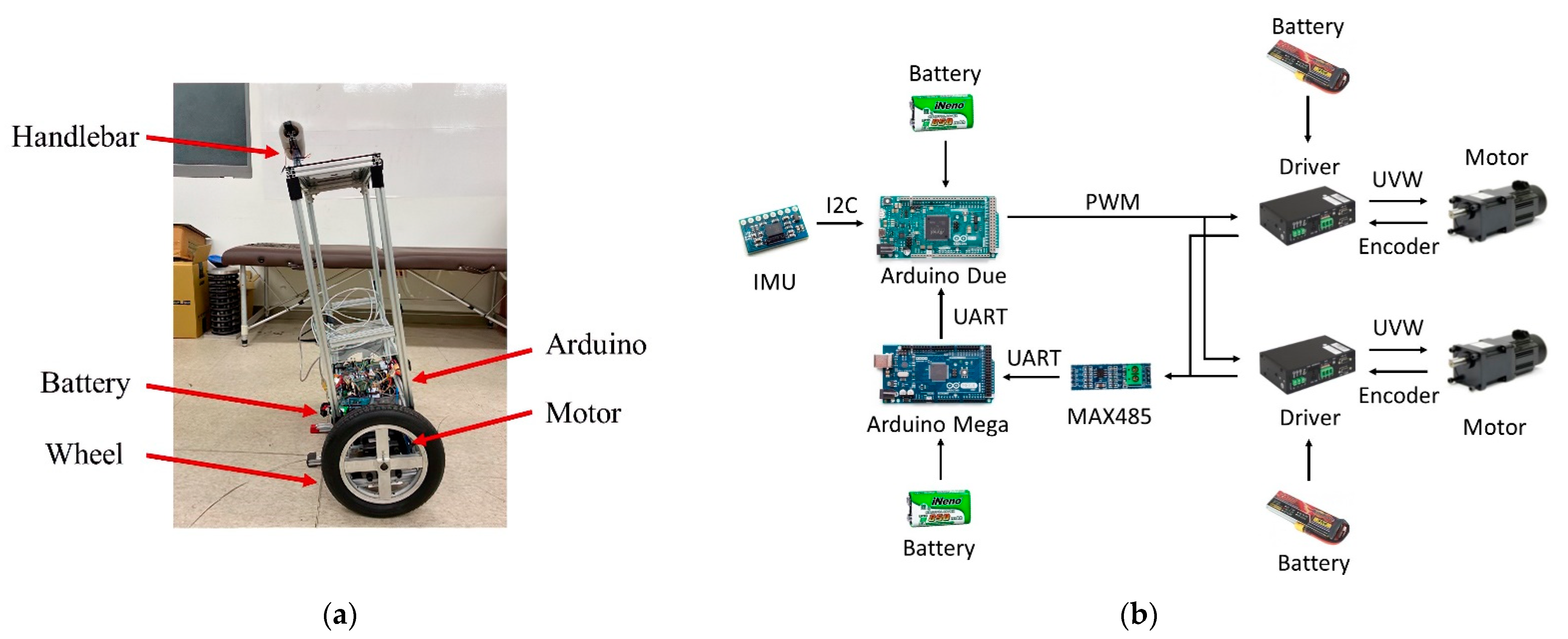
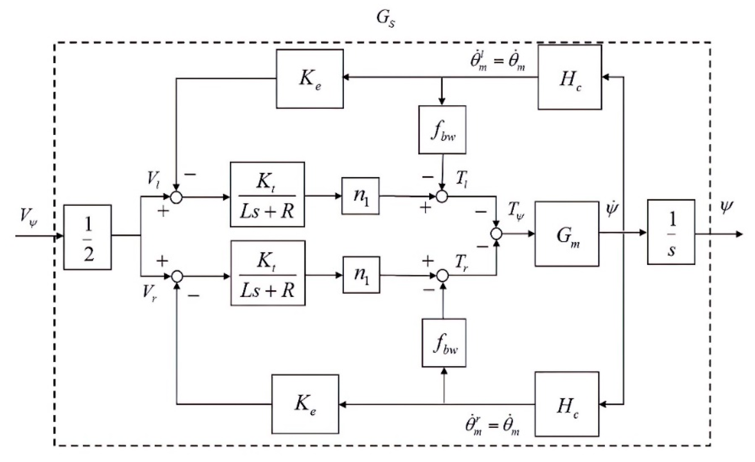
2. System Description and Modeling

The TWIP system shown in Figure 1a equips the two wheels driven by direct current (DC) motors [32] with absolute rotary encoders. We applied an inertial measurement unit (IMU) [33] to measure the body motions and implemented the controllers on an Arduino Due microcontroller with a sampling time of 0.025 s [34]. Each motor consumed an average power of about 9 watts, so we implemented two 22.2 V/2600 mAh Li-Po batteries to sustain the system operation for about 6 h. The system architecture is shown in Figure 1b, while the system specifications are illustrated in Table 1. Note that some parameters in Table 1 were estimated by software packages. For example, the inertial moments Jψ and J ϕ were estimated by using Solidwork and SimMechanics. We drew the design in Solidwork then converted it to a SimMechanics model, which could calculate the theoretical inertial moments. The friction fbw was estimated from the steady-state responses. We assumed that the motor output torque was equivalent to the friction torque in the steady-state responses, so that we could calculate fbw by the input voltage and the angular velocity of the motor.
The mathematical model of the TWIP system is derived in Appendix A. Considering the translational motion of the TWIP system, the block diagram of the model can be illustrated in Figure 2, in which
H c = L { θ ˙ m } L { ψ ˙ } = s θ ^ m s ψ ^ = [ ( 2 m + M ) r 2 + 2 J w + 2 M r l + M l 2 + J ψ ] s 2 + M g l [ ( 2 m + M ) r 2 + M r l + 2 J w ] s 2
G m = s ψ ^ T ^ ψ = [ ( 2 m + M ) r 2 + M r l + 2 J w ] s [ ( 2 m + M ) r 2 + 2 J w + 2 n 1 2 J m ] [ ( M l 2 + J ψ + 2 n 1 2 J m ) s 2 M g l ] ( M r l 2 n 1 2 J m ) 2 s 2
where f ^ ( s ) = L { f ( t ) } represents the Laplace transform of f ( t ) . ψ is the pitch angle of the cart, θ is the wheels’ rotational angle, θ m is the motor’s rotational angle, and T ^ ψ is the applied torque to the cart. Substituting the system parameters shown in Table 1, the system transfer function from the motor voltage to the pitch angle of the cart can be described as follows:
G S = ψ ^ V ^ ψ = 9106 s s 4 + 473.8 s 3 + 4402 s 2 5994 s 3.423 × 10 4

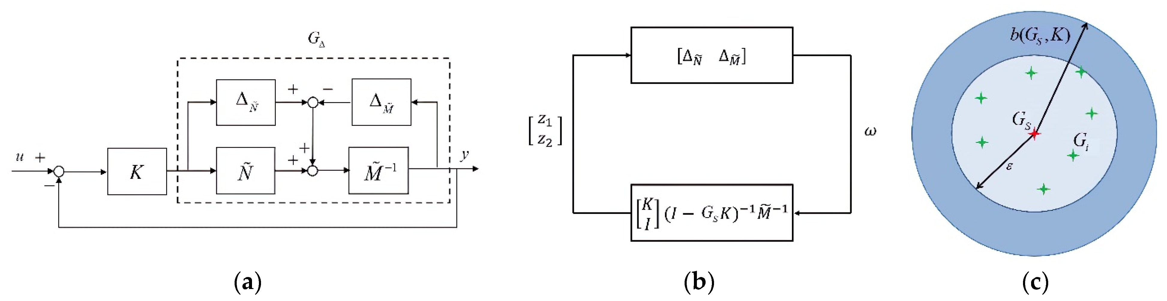
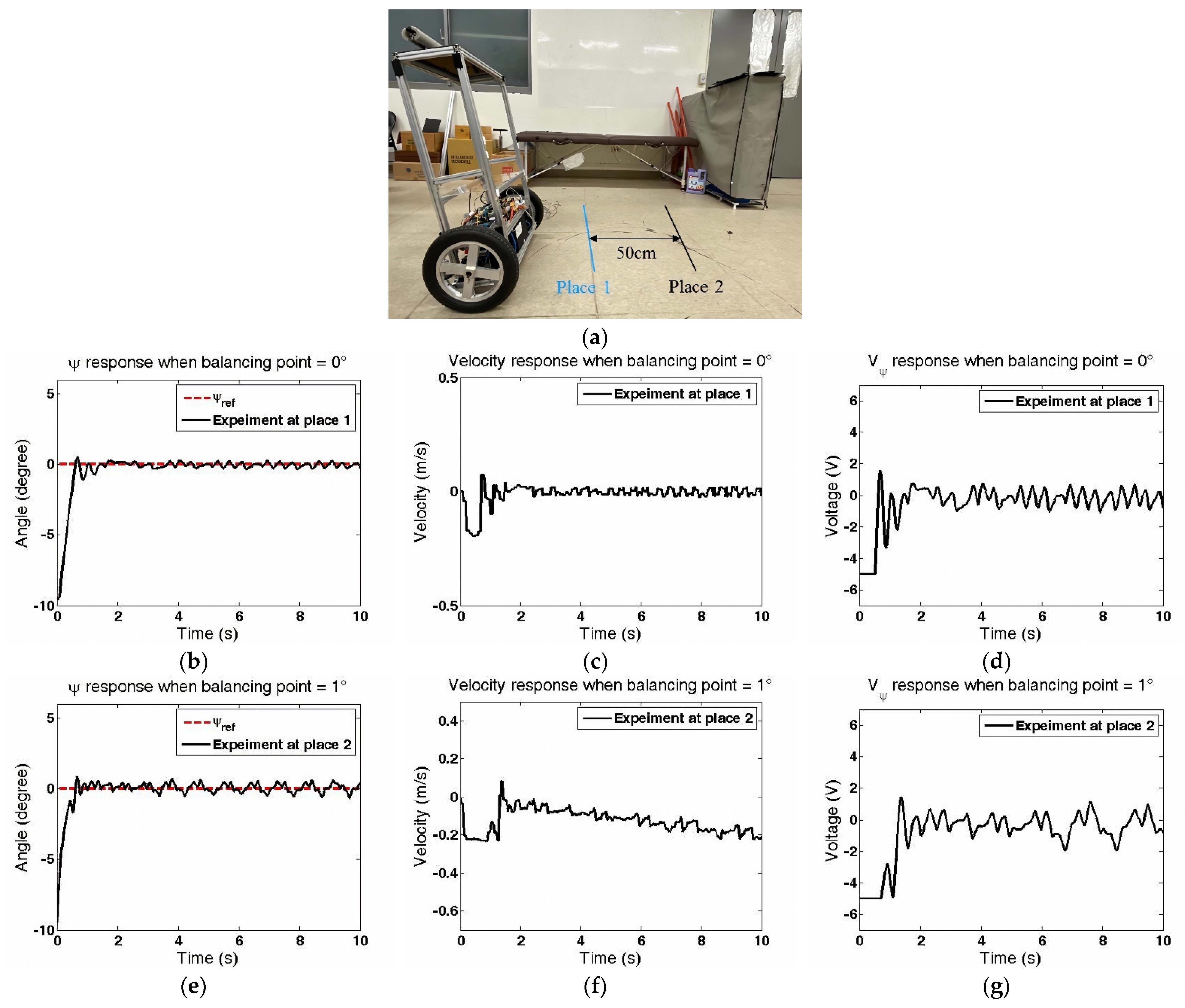
3. Robust Loop-Shaping Control Design for System Stability

This section applies robust loop-shaping control to stabilize the TWIP system. The model in Equation (3) represents a linear system, so we can regard system nonlinearities and variations during operation as model uncertainties and apply robust control to cope with these uncertainties. Suppose the transfer function G S of Equation (3) can be represented by the following normalized left coprime factorization [35]:
G S = M ˜ 1 N ˜
in which M ˜ , N ˜ R H and M ˜ M ˜ * + N ˜ N ˜ * = I . A perturbed plant G Δ can be described as follows:
G Δ = ( M ˜ + Δ M ˜ ) 1 ( N ˜ + Δ N ˜ )
where Δ M ˜ , Δ N ˜ R H . The gap between the nominal plant G S and the perturbed plant G Δ is defined as [35]: The smallest value of [ Δ M ˜ Δ N ˜ ] that perturbs G P o into G P Δ is denoted as δ ( G S ,   G Δ ) . The closed-loop system with a perturbed plant G Δ and a controller K can be expressed as in Figure 3a. As system stability is independent of the input and output of the system, we can rearrange the system block diagram, as in Figure 3b. From the Small Gain Theorem [36], the closed-loop system is internally stable for all perturbations with [ Δ M ˜   Δ N ˜ ] ε if, and only if,
[ K I ] ( I G S K ) 1 M ˜ 1 = [ K I ] ( I G S K ) 1 [ I G S ] < 1 ε
Hence, we can define the system’s stability margin b ( G S , K ) as follows [36]:
b ( G S , K ) = [ K I ] ( I G S K ) 1 [ I G S ] 1
The system is internally stable for all uncertainties Δ with Δ = [ Δ M ˜   Δ N ˜ ] ε if and only if b ( G S , K ) > ε . The philosophy of robust control design can be illustrated as in Figure 3c for the design of a controller K for the nominal plant G S such that the stability margin b ( G S , K ) is greater than the system perturbation [ Δ M ˜   Δ N ˜ ] . We consider the model of (3) with the following variations: (i) friction f b w [ 0 ,   3 ] Nms/rad; (ii) height of the center of gravity l [ 0.2 ,   0.4 ] m; and (iii) mass M [ 13 ,   1 5 ] kg. We divide each variation into ten equivalent sections and calculate the system perturbation between these 113 models and the nominal model G S . The maximum system perturbation [ Δ M ˜   Δ N ˜ ] is found to be 0.180. Therefore, the designed robust controller should have a stability margin greater than 0.180 to guarantee system stability during operations.
Figure 3. System perturbations and stability analyses: (a) The closed-loop system; (b) System rearrangement; (c) The philosophy of robust control.
Machines 09 00205 g003
The principles of loop shaping [37] can be summarized as follows: (i) increasing system gains at the low-frequency ranges for disturbance rejection; (ii) decreasing system gains at the high-frequency range for attenuating noises; (iii) limiting the slope of the magnitude plots around crossover frequencies less steep than −40 dB/decade for stability considerations. Referring to the nominal plant of (3), we iteratively adjusted the weighting functions and verified the system performance by experiments. That is, we set the weighting functions and implemented the derived controllers for simulation and experiments. Then, we checked the system performance, such as the overshoot, steady state error, and settling time. The controller should be a compromise between these performance considerations. Finally, we selected the following weighting function:
W ψ = 200 1 0.01 s + 1
and applied the MATLAB command ncfsyn (ncfsyn designs an optimal controller that provides the maximum stability margin for the weighted plant) to design the robust controller, as follows:
K ψ = 3.044 s 4 1804 s 3 + 1.905 × 10 5 s 2 4.116 × 10 6 s + 4.584 × 10 5 s 4 + 705.9 s 3 + 1.36 × 10 5 s 2 + 1.234 × 10 7 s 1.506 × 10 5
which gives a stability margin of b ( W ψ G S , K ψ ) = 0.4018 . As the stability margin is greater than the system gap of 0.180, system stability can be guaranteed during operations. Note that any parameter variation can be considered in a similar way. The designed controller can cope with mixed parameter variations as long as the gap between the perturbed model G Δ and the nominal plant G S is less than the stability margin, i.e., δ ( G S , G Δ ) < 0.4018 .
We implemented the designed controller W ψ K ψ on MATLAB for simulation with a fixed sampling time of 0.025 s. The balance loop control structure is shown in Figure 4a, where the voltage saturation function was set as | V ψ | 5 volts based on the hardware constraints. We set the initial angle of ψ ( 0 ) = 9.5 ° and ψ r e f = 0 ° , i.e., assuming the balancing point was zero. The system responses are shown in Figure 4b,c, where both the pitch angle ψ and the forward velocity approached zero when the system is balanced. The corresponding control signal is illustrated in Figure 4d, where the saturation function was activated before 0.25 s to balance the TWIP system from the initial position ψ ( 0 ) = 9.5 ° . Suppose the reference balancing point varied from 0° to 1° because of model variations and disturbances; the system responses are shown in Figure 4e–g. Figure 4e showed that the pitch angle ψ still approached zero because of the reference command ψ r e f = 0 ° . However, the forward velocity drifted because the real balancing point was changed to 1°. For example, the negative slope shown in Figure 4f indicated that the TWIP robot moved backward in order to maintain balance. That is, the TWIP system cannot be statically balanced if the reference ψ r e f differs from the system’s balance point, which might vary during operations. Therefore, ψ r e f should be adjusted in real time according to the operating conditions. Figure 4g showed that the control signal was saturated at the first 0.1 s because the TWIP robot needs to be balanced from ψ ( 0 ) = 9.5 ° to 0 ° .
We also implemented the designed control on the microcontroller for experiments. The experimental setting is shown in Figure 5a, where the TWIP was set to balance at two locations from an initial angle of ψ ( 0 ) = 9.5 ° . Considering the balance control loop shown in Figure 4a with ψ r e f = 0 ° , the experimental responses are illustrated in Figure 5. At place 1, the pitch angle approached zero, but the velocity oscillated around zero when the system was balanced. The situation was more noticeable at place 2, where the velocity was drifting (see in Figure 5e) because the reference ψ r e f differed from the system’s balance point. Figure 5f showed that the control signal was saturated at the first 0.1 s because the TWIP robot needs to be balanced from ψ ( 0 ) = 9.5 ° to 0 ° .
Both simulation and experimental results (see Figure 4 and Figure 5) suggest that the balancing point has changed because of model variations and disturbances. That is, the reference command ψ r e f should be adjusted in real-time. Therefore, we propose a multi-loop control structure in the next section to update the reference angle ψ r e f in real-time.

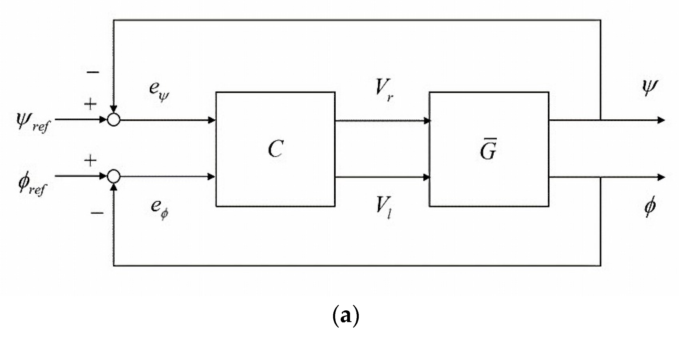
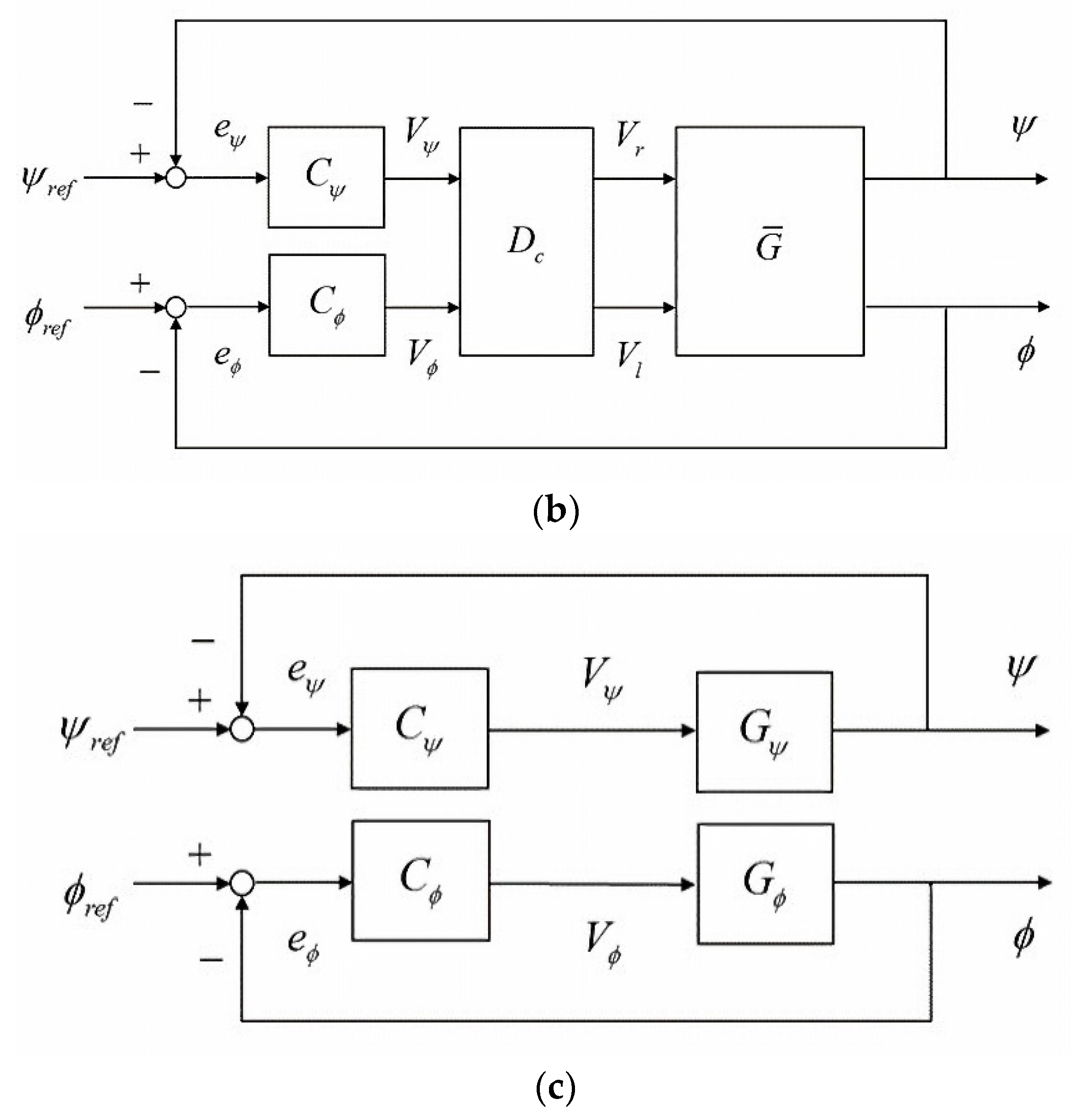
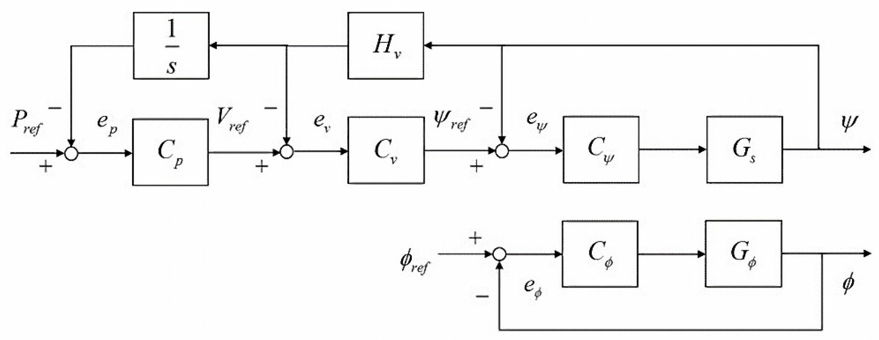
4. The Multi-Loop Control Structure

This section proposes a multi-loop control structure to solve the velocity-drifting problem of the TWIP system. The multi-loop structure is composed of a velocity loop and a position loop. The velocity loop can regulate the forward velocity and adjust the reference angle in real-time, while the position loop control can achieve position tracking. We design the corresponding controllers and demonstrate the effectiveness of this control structure by simulation and experiments.

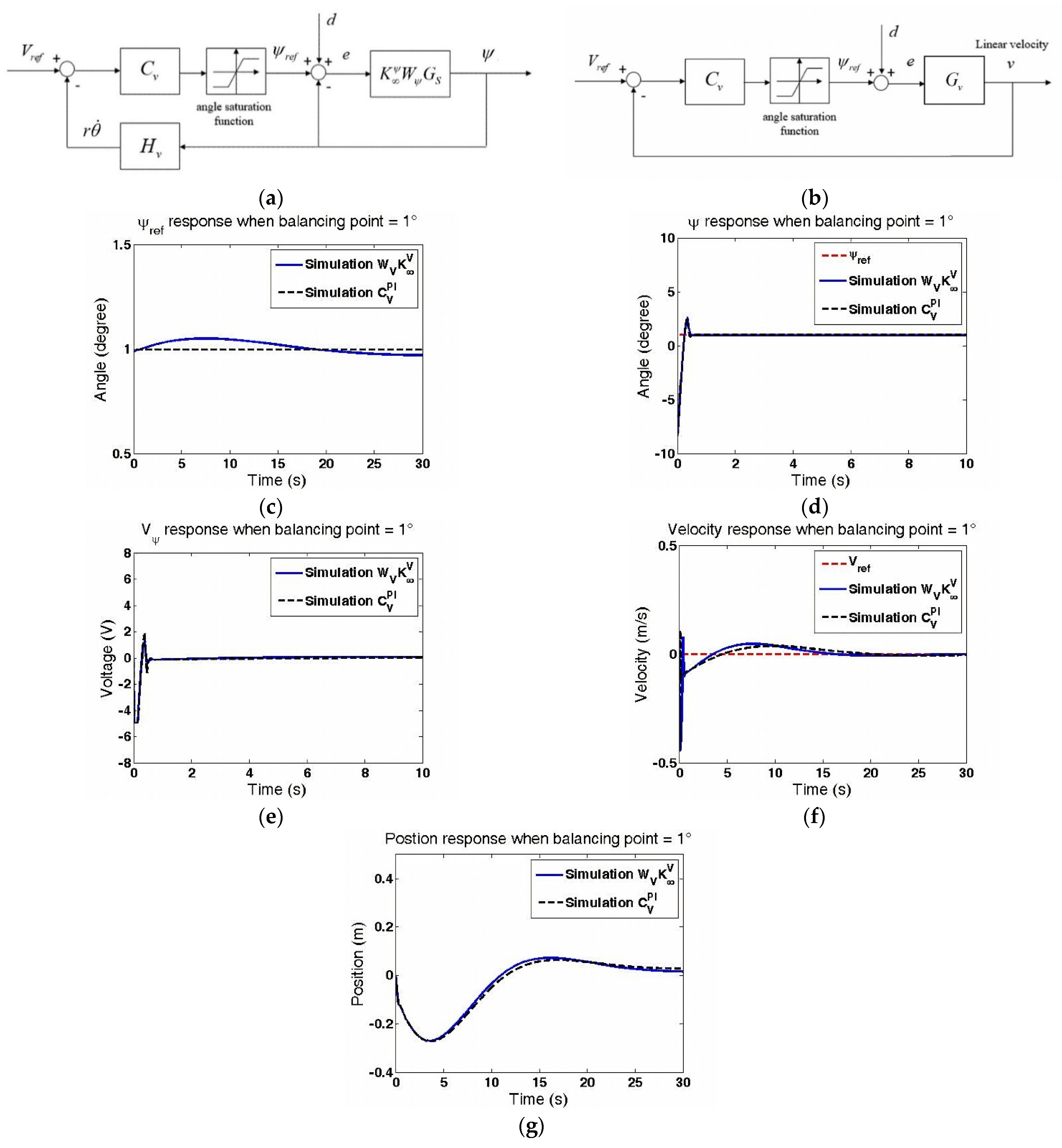
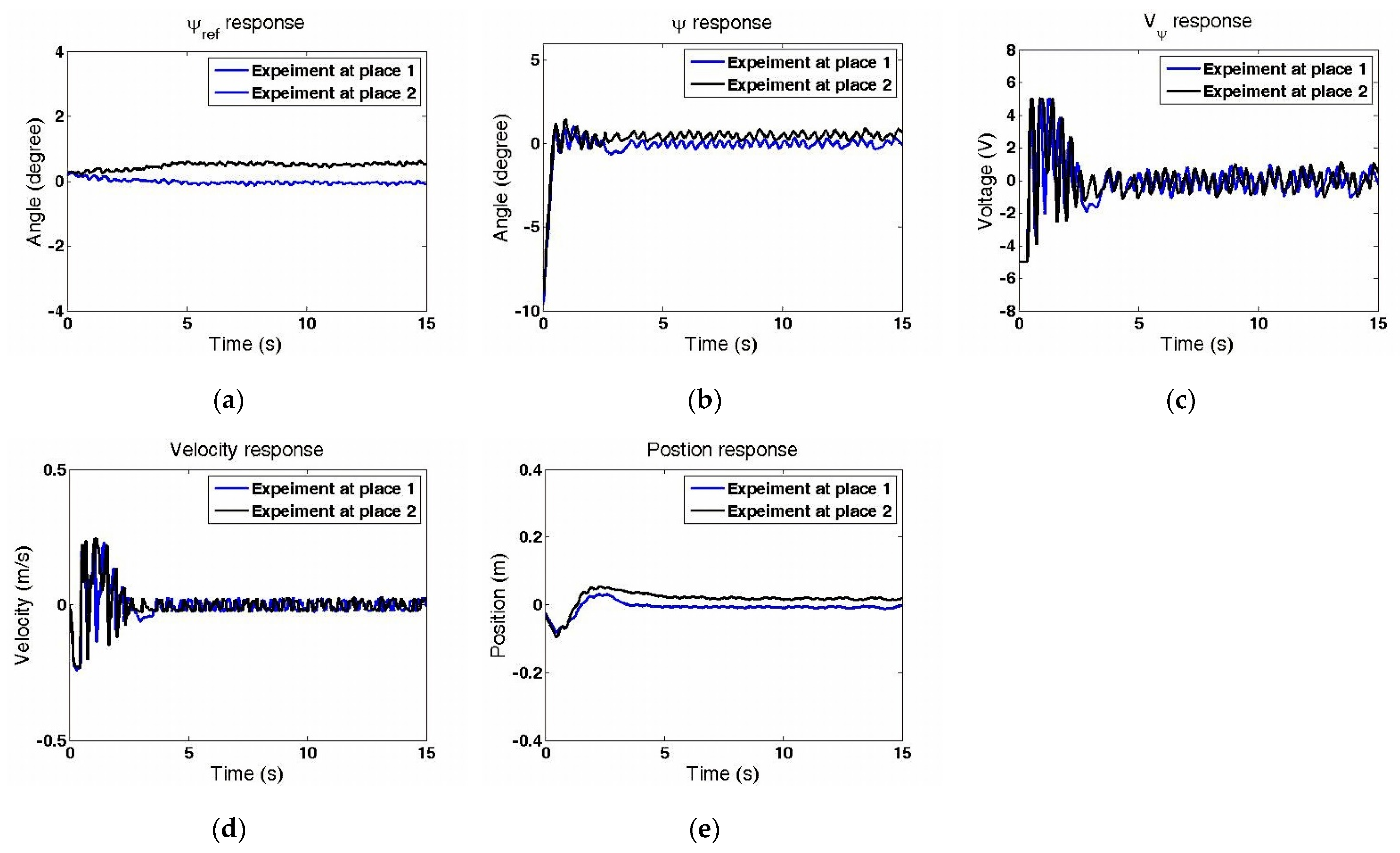
4.1. The Velocity Loop Control

We apply a velocity loop control structure to adjust the reference angle ψ r e f , as shown in Figure 6a. If the TWIP system is statically balanced, the pitch angle should approach the balancing point and the linear velocity should converge to zero. The following calibration function H v is derived in Appendix A:
H v = r s θ ^ ψ ^ = r [ ( J ψ + M l 2 + M r l ) s 2 + M g l ] [ ( 2 m + M ) r 2 + M r l + 2 J w ] s
The block diagram of Figure 6a can be simplified as in Figure 6b, where
G v = K ψ W ψ G S 1 + K ψ W ψ G S H v
We applied the modified plant G v to design the velocity controller C v by robust loop-shaping techniques, where the weighting function was iteratively tuned and verified. Finally, we selected the following weighting function:
W v = 0.01 0.5 s + 0.03
to derive the robust controller, as follows:
K v = 2.358 s 7 + 1668 s 6 + +   8.922 × 10 9 s + 5.708 × 10 8 s 7 + 708.3 s 6 + + 1.401 × 10 10 s + 1.36 × 10 9
As the weighted controller C v = W v K v was eighth-order and might increase the difficulties of hardware implementation, we considered the following proportional-integral (PI) control:
C v = C v P I = K p + K i s = K p s + K i / K p s
The values of K p and K i were tuned to provide similar responses to those of the standard robust controller. Finally, we selected the following PI controller:
C v = C v P I = 0.0335 s + 1 s
We implemented the designed controllers on MATLAB for simulation. We set V r e f = 0 with a balancing point of 1° and applied the angle saturation function to limit the reference angle as | ψ r e f | 3 ° . Suppose the initial angle is ψ ( 0 ) = 9.5 ° ; the simulations are shown in Figure 6. First, the PI control achieved similar responses to the standard robust controller, but with a much simpler form. Second, ψ r e f was successfully adjusted to the balancing point (see Figure 6c), while the pitch angle ψ approached 1° (see Figure 6d). Third, the corresponding control signal is shown in Figure 6e, where the saturation function was activated before 0.2 s to balance the system from ψ ( 0 ) = 9.5 ° to ψ r e f . Fourth, the forward velocity converged to zero, as illustrated in Figure 6f, i.e., the system was statically balanced by the velocity loop. Lastly, Figure 6f showed that the displacements were oscillating, so that we needed to add a position loop to improve position tracking.
We also implemented the velocity loop control for experiments. We applied the PI controller of Equation (15) to simplify hardware implementation, because it provided similar responses to the standard robust controller but with a much simpler form. We set the TWIP system at the two locations (see Figure 5a) with an initial angle of ψ ( 0 ) = 9.5 ° and a reference velocity V r e f = 0 . The experimental results are shown in Figure 7. First, Figure 7a shows that the velocity loop adjusted the reference balance point in real-time, while Figure 7b shows how the pitch angle ψ tracked the reference angle ψ r e f . Second, the motor control signal V ψ was frequently saturated at the first two seconds, as shown in Figure 7c, to balance the TWIP robot from the initial angel of ψ ( 0 ) = 9.5 ° . Third, the velocity approached zero, as shown in Figure 7d (i.e., the system was statically balanced). However, Figure 7e shows that the TWIP was statically balanced at different positions, which cannot be specified. This problem can be solved by the position loop control.

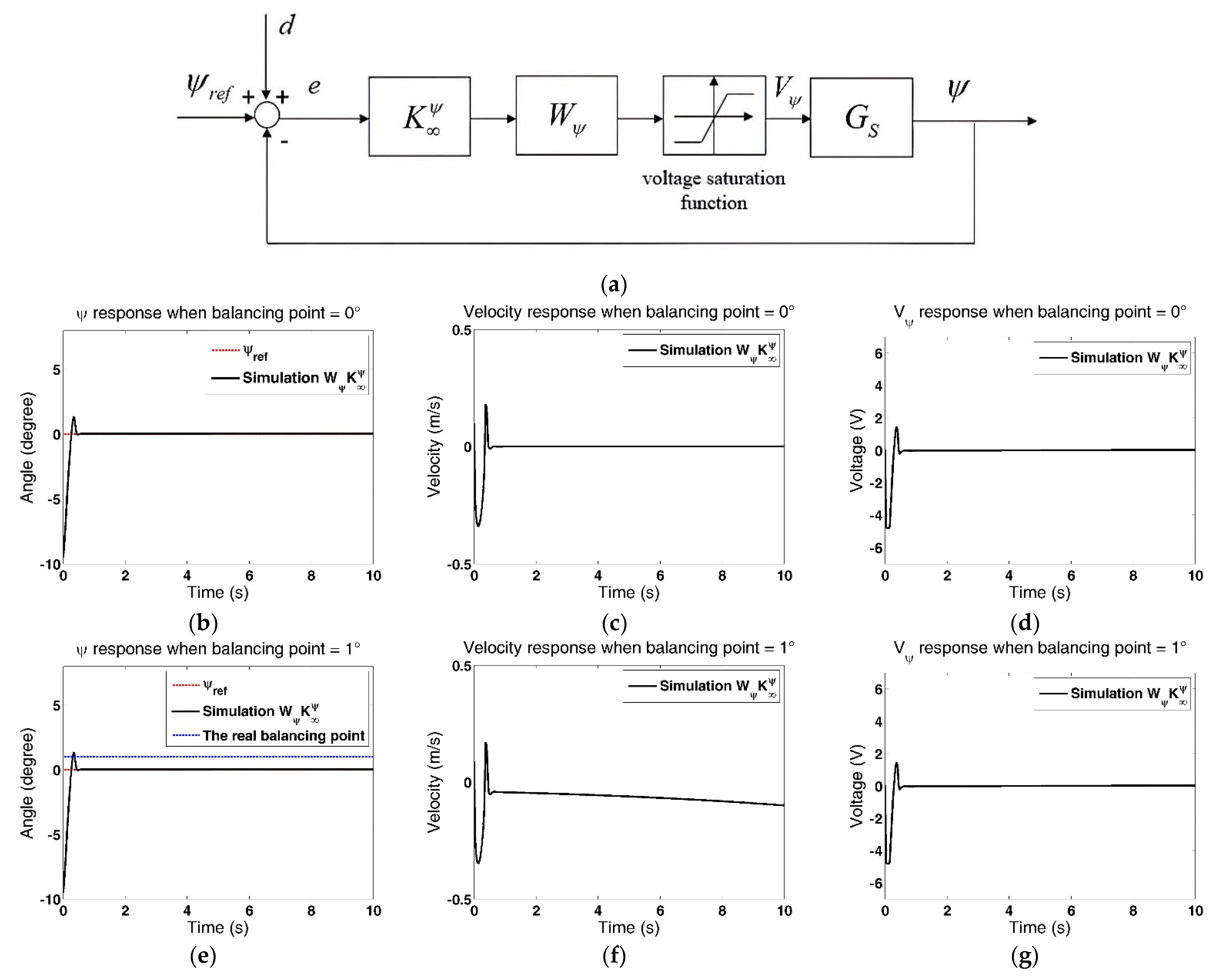
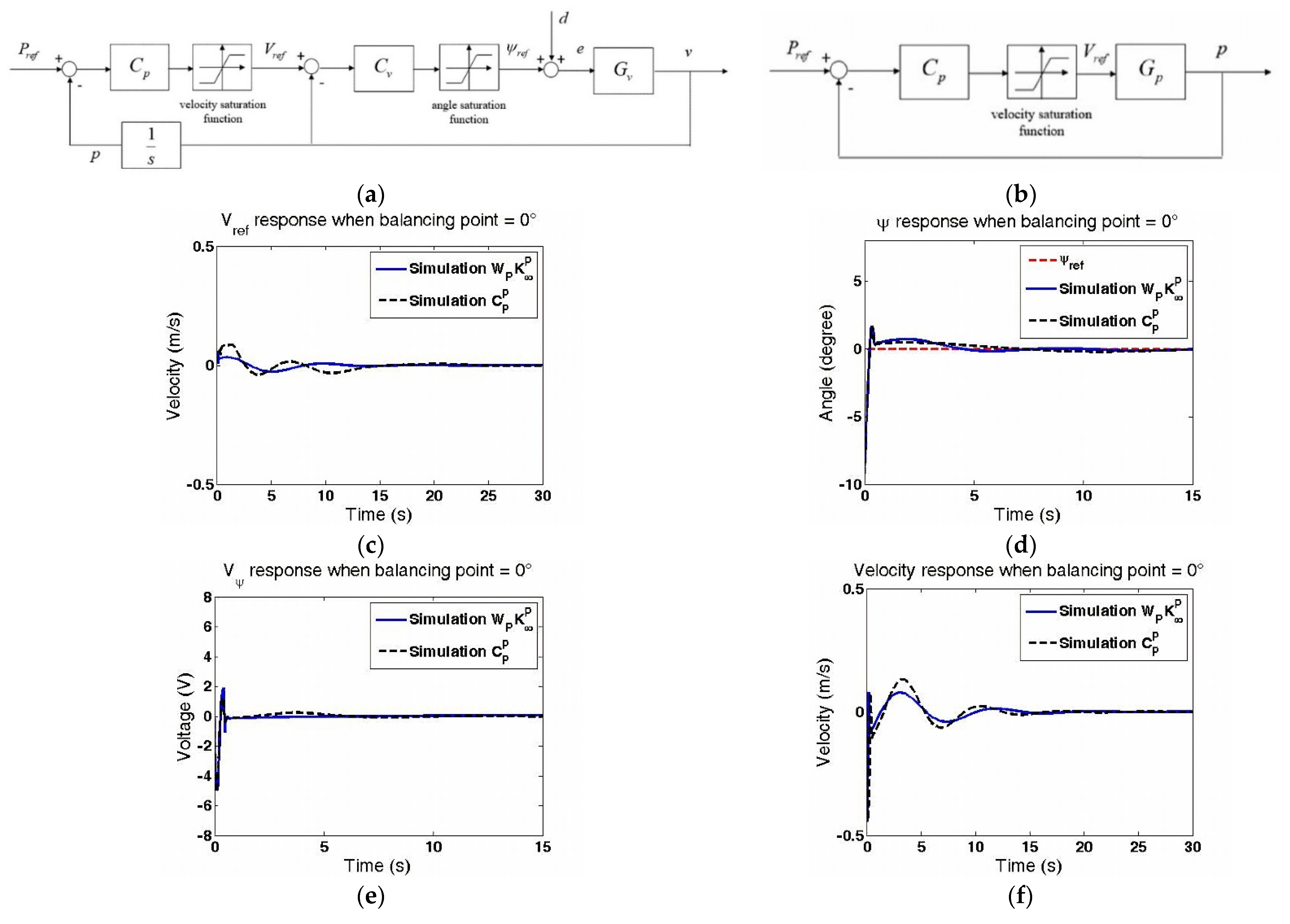
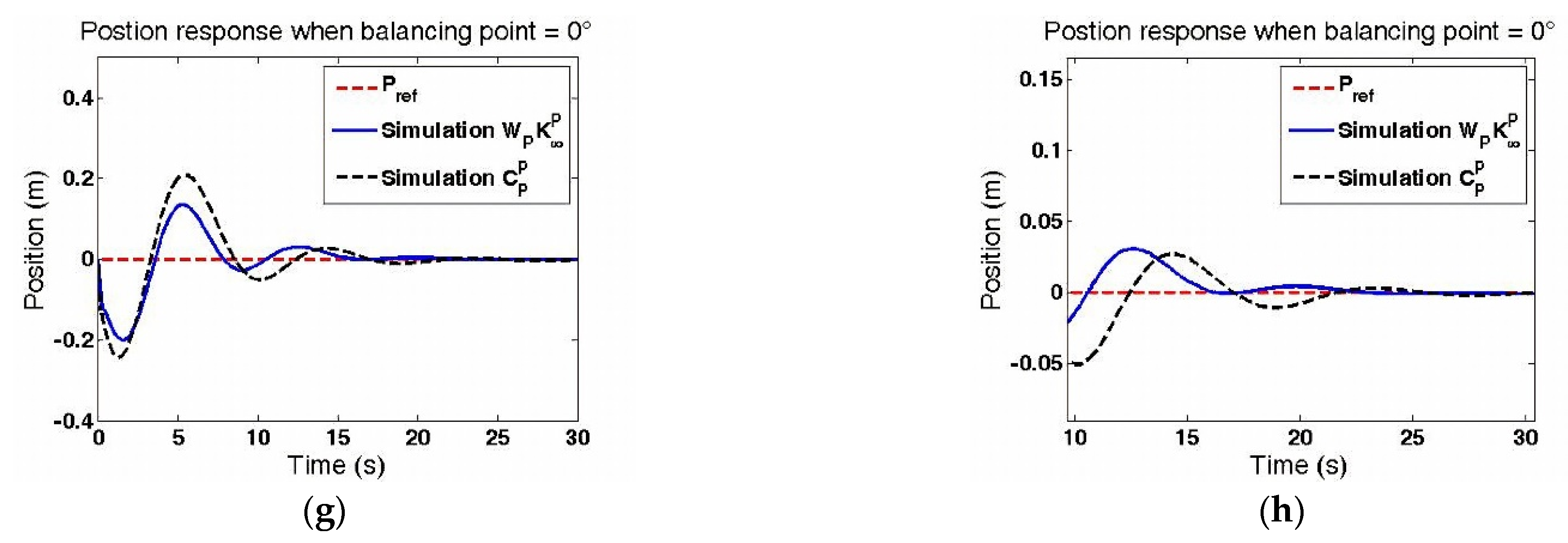
4.2. The Position Loop Control

The position-loop control structure is shown in Figure 8a, where the velocity command V r e f can be adjusted according to the position error. We set a velocity saturation function | V r e f | 0.3 m/s to limit the maximum speed, considering the motor power. Figure 8a can be further simplified as Figure 8b, where the modified plant G p is:
G p = C v G v ( 1 + C v G v ) s
We also applied robust loop-shaping control to the position control, with the following weighting function:
W p = 0.8 s + 0.25 0.45 s 2 + 0.3 s + 0.1
The robust controller was designed as follows:
K p = 5.115 s 12 + 1164 s 11 +   1.611 × 10 5 s + 4703 s 12 + 229.5 s 11 + + 7.694 × 10 5 s + 2.406 × 10 4
As the order of the robust controller C p = W p K p was fourteen and might cause difficulties in hardware implementation, we further considered the following proportional controller for the position loop:
C p = C p P = 0.09
This provided system responses similar to the standard robust controller but with a much simpler form. We implemented the designed control on MATLAB for simulation. We set P r e f = 0 with a balance point of 0° and an initial pitch angle ψ ( 0 ) = 9.5 ° . The simulation results are shown in Figure 8. First, the responses employing the proportional control and the robust control are similar, allowing us to simplify the control implementation using the proportional control for the experiments. Second, Figure 8c shows that the reference velocity was adjusted in real-time, and the system was statically balanced. Third, the pitch angle ψ approached zero (see Figure 8d) with the corresponding control shown in Figure 8e. Finally, the linear velocity v approached zero (see Figure 8f) and the position p also converged to zero, as shown in Figure 8f, indicating that the TWIP can remain at specified places. Figure 8h shows the zoom-in position responses, which slightly oscillated before converging to zero.
We also implemented the designed control on a microcontroller for experimental verification. We applied the P controller of (19) to simplify hardware implementation, because it provided similar responses to the standard robust controller but with a much simpler form. We set P r e f = 0 with an initial angle ψ ( 0 ) = 9.5 ° , and we set the saturation functions | ψ r e f | 3 ° and | V r e f | 0.3 m/s. The experimental results are shown in Figure 9. First, the position loop adjusted the reference velocity V r e f in real-time, as illustrated in Figure 9a. Second, Figure 9b shows that the angle ψ approached to the balancing point. Third, the corresponding control signal is shown in Figure 9c, where the motors continuously regulated the velocity and position of the TWIP robot. Fourth, the forward velocity approached zero (see Figure 9d), while the TWIP remained at the starting place (see Figure 9e). Figure 9f shows the zoom-in position responses after settling, where the TWIP robot oscillated within about ±1 cm. Finally, the statistical data are shown in Table 2, where the mean absolutely error (MAE) and the root mean square error (RMSE) after the settling time are defined as
MAE 1 T t s t = t s T | e ( t ) | d t
RMSE ( 1 T t s t = t s T | e ( t ) | 2 d t ) 1 / 2
in which e indicates the corresponding error, T = 15 s, and t s is the settling time, when the error of the pitch angel is less than 0.475 o (i.e., 5% of the step from 9.5 ° to 0 ° ) afterwards. From the table, in place 1 and place 2, the rise time were 0.4 s, while the MAE and RMSE of ψ were less than 0.178° and 0.224°, respectively. The position responses converge to zero with an MAE of less than 8.9 mm and an RMSE of less than 9 mm. That is, the TWIP system can be statically balanced at specified positions by the proposed multi-loop control layout.

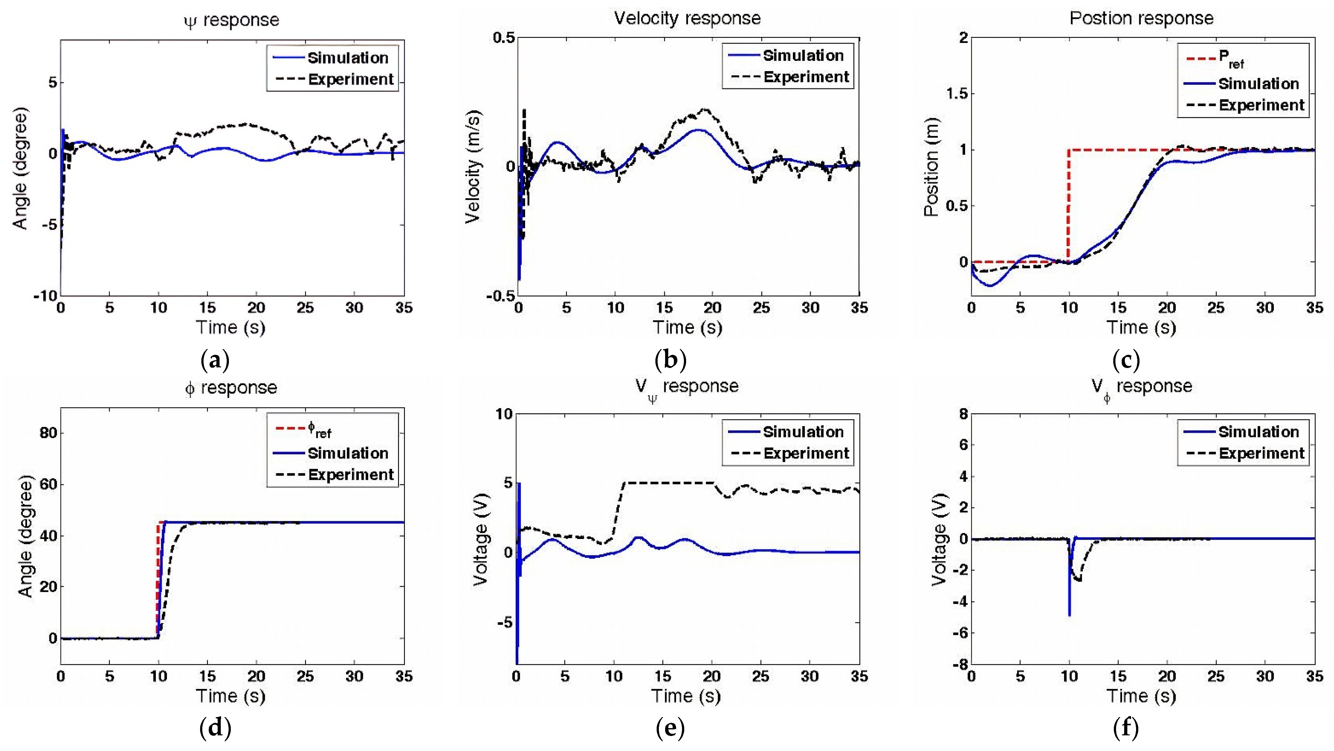
5. Decoupled Control Loops

The TWIP system consists of two control loops: the balance loop and the steering loop. The balance control loop stabilizes the system, while the steering control loop regulates the movement direction, as illustrated in Figure 10a. This section proposes a method to decouple these two control loops. From Appendix A, the transfer function matrix from the motor voltages ( V r and V l ) to the balancing angle ψ and the steering angle ϕ can be represented as follows:
[ ψ ϕ ] = G ¯ [ V r V l ] = [ G 21 G 22 G 31 G 32 ] [ V r V l ]
where G 22 = G 21 and G 31 = G 32 . Suppose the system of Figure 10a can be rearranged as Figure 10b with
C = D c [ C ψ 0 0 C ϕ ] ,   D c = [ D 11 D 12 D 21 D 22 ] ,
by a suitable D c . That is, the transfer function matrix from input motor voltages ( V ψ and V ϕ ) to the output angles ( ψ and ϕ ) are as follows:
[ ψ ϕ ] = G ¯ [ V r V l ] = G ¯ D c [ V ψ V ϕ ] = [ G 21 G 22 G 31 G 32 ] [ D 11 D 12 D 21 D 22 ] [ V ψ V ϕ ]              = [ D 11 G 21 + D 21 G 22 D 12 G 21 + D 22 G 22 D 11 G 31 + D 21 G 32 D 12 G 31 + D 22 G 32 ] [ V ψ V ϕ ]
Therefore, the system can be decoupled if the following two off-diagonal terms are zeros:
V ψ ( D 11 G 31 + D 21 G 32 ) = 0
V ϕ ( D 12 G 21 + D 22 G 22 ) = 0
As G 22 = G 21 and G 31 = G 32 , we can set D 21 = D 11 = 0.5 and D 12 = D 22 = 0.5 to decouple the two control loops. Furthermore, we define G ψ = G 21 = G 22 and G ϕ = G 32 = G 31 , which represent the balance sub-model and the steering sub-model, respectively. Substituting Equations (25)–(26) into Equation (24) gives:
ψ = ( D 11 G 21 + D 21 G 22 ) V ψ = G ψ V ψ
ϕ = ( D 12 G 31 + D 22 G 32 ) V ϕ = G ϕ V ϕ
as shown in Figure 10c. That is, the balancing loop and the steering loop can be decoupled and independently controlled.
We can further integrate the balancing loop with the aforementioned velocity and position loops, as shown Figure 11. Substituting the parameters of Table 1, the balancing sub-model is G ψ = G s , as shown in Equation (3), while the steering sub-model is:
G ϕ = G 32 = 2.117 × 10 4 s 3 + 474.2 s 2 + 2955 s
Similarly, we applied robust loop-shaping control to G ϕ and selected the following weighting:
W ϕ = 10 0 . 01 s + 1
The robust controller C ϕ = W ϕ K ϕ was derived, where
K ϕ = 2.278 s 2 253 s 2724 s 2 + 147.4 s + 6209
We implemented the designed controllers in Figure 11 to demonstrate the position tracking of the TWIP system. Suppose the TWIP is balanced and then given a target on the forward left, with an angle of 45° and a distance of 1 m; the system responses are shown in Figure 12. First, the system remains balanced during the tracking process, as shown in Figure 12a. Second, the velocity and position responses are illustrated in Figure 12b,c, respectively. Third, the steering response is shown in Figure 12d and is much faster than the position/velocity/balance responses because the steering loop is independently controlled. The motor voltages, V ψ and V ϕ , are illustrated in Figure 12e,f, where the TWIP robot made a swift turn at t = 10 then moved forward until it reached the target position and settled there according to the control loop.

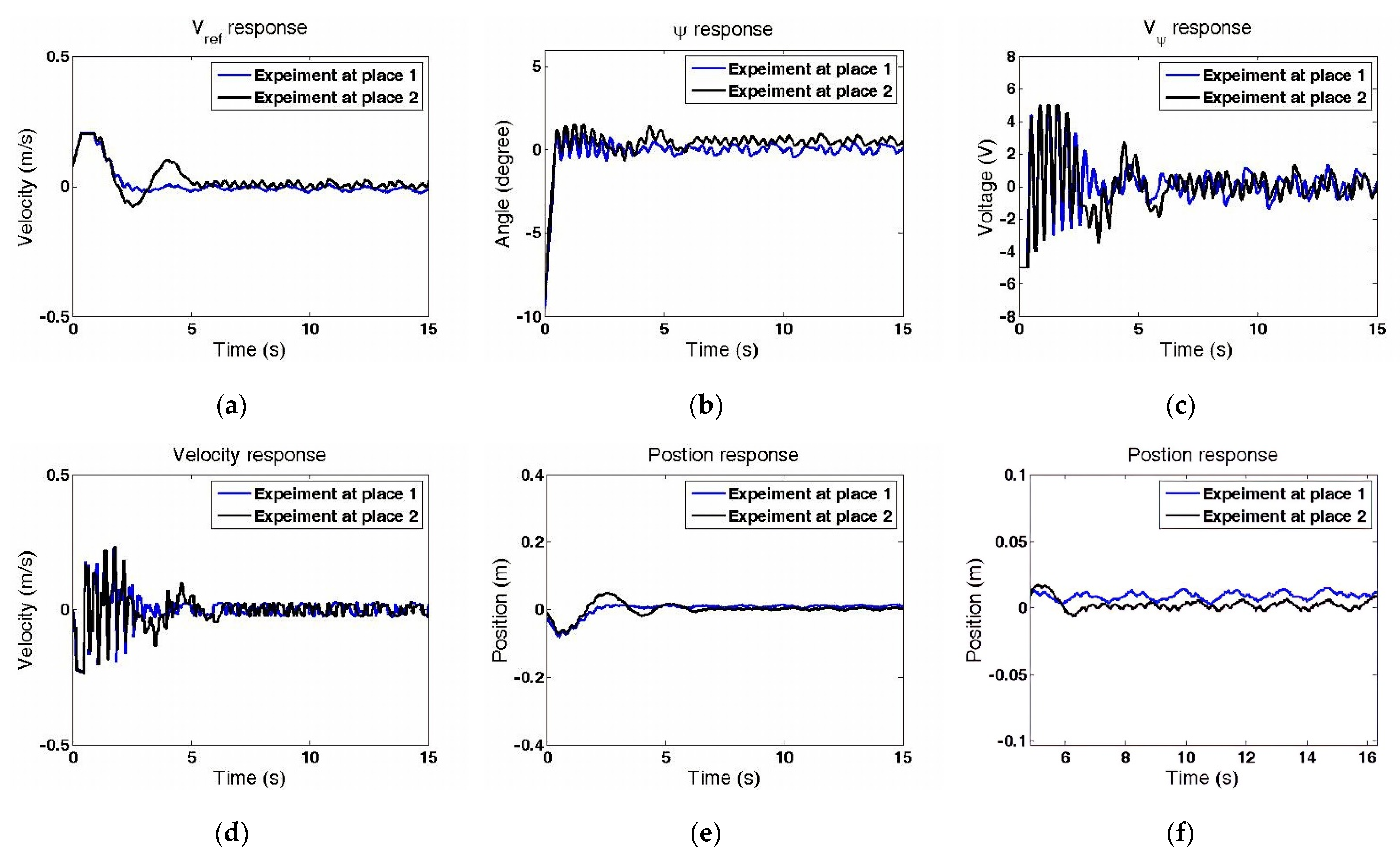
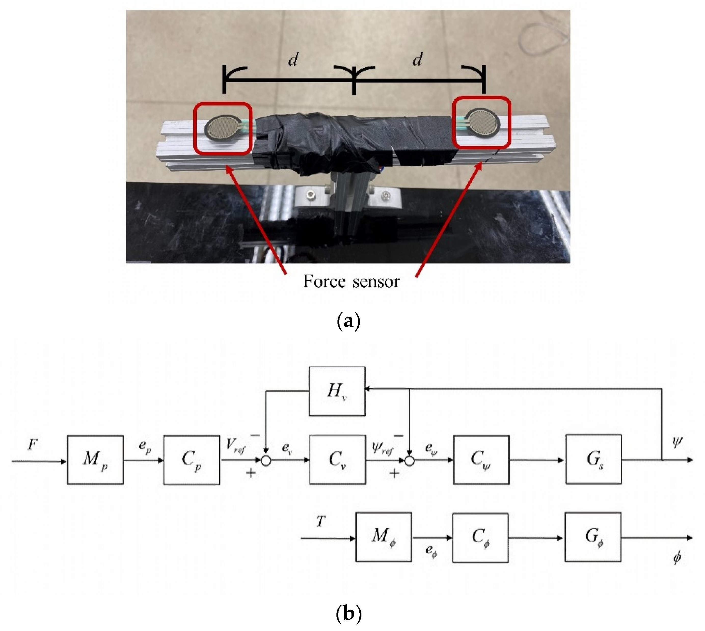
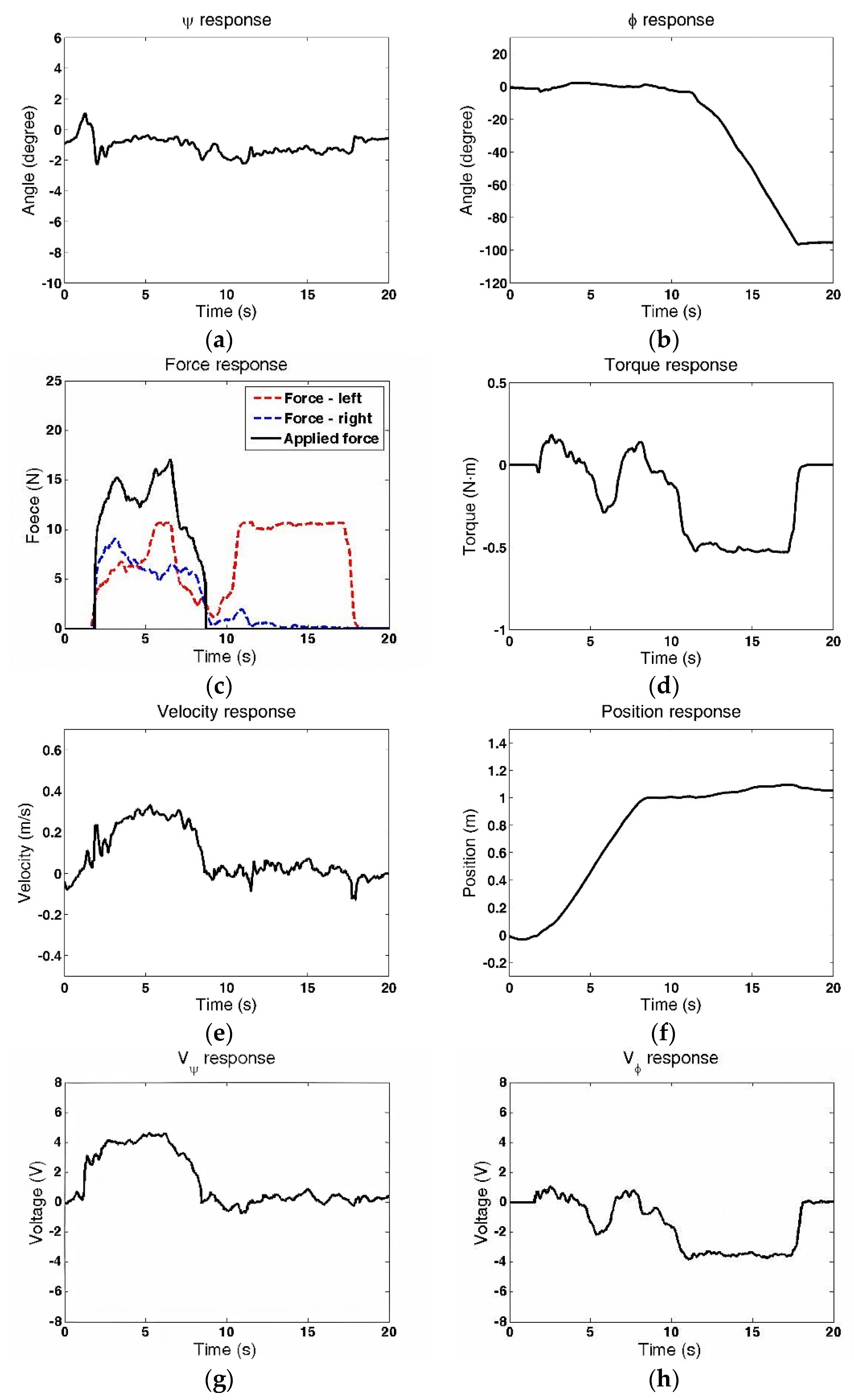
Walking Assistance by the TWIP Robot

We applied the TWIP robot to assist users with walking. The TWIP provides physical support to the user during motion, while the user gives commands based on visual feedback. We implemented two force sensors [38] on the handrail, as shown in Figure 13a, so that the users can control the direction of the TWIP robot by applying forces to the handrail. Suppose F l and F r represent the measured forces on the left and the right sensors, respectively. The applied force F and torque T are estimated as:
F = { F l + F r ,   if   min { | F l | , | F r | } 2 N 0 ,                 otherwise
T = F r d F l d
where d is the distance between the force sensors and the center of the handrail. We set a threshold of 2 N to filter disturbances when estimating the user’s intention. The force F is then transferred to an motion error e P by a function M P , while the torque T is transferred to an rotational command by the function M ϕ , as shown in Figure 13b. We set M P = 0.007 so that the TWIP robot moves at a speed of about 0.4 m/s when the applied force F is about 15 N. Similarly, we set M ϕ = 0.1 so that the TWIP robot rotates at an angular velocity of about 15 degree/s when the applied torque T is about 0.5 Nm.
We conducted experiments to demonstrate the walking assistance function of the TWIP robot. The user was asked to walk in a straight line and then turn 90 ° to the right [39]. The system responses are illustrated in Figure 14. First, the TWIP robot remained stable during the whole process of assisting with walking, as shown in Figure 14a. That is, the designed robust controller can cope with the system uncertainties and disturbances during motion. Second, when the force sensors detected the applied force (see Figure 14c), the robot began to move forward and remained stable using the designed decoupled multi-loop control. Lastly, the robot allowed a right turn (see Figure 14b) when a torque of about −0.5 Nm was estimated at around 11 s, as shown in Figure 14d, indicating that the user intended to make a right turn. Note that the applied force was estimated as zero, because the right sensor force F r was less than 2N. Therefore, the parallel-wheel structure allowed the robot to turn on the spot, as illustrated in Figure 14e,f. The corresponding motor control voltages, V ψ ( t ) and V ϕ ( t ) , are shown in Figure 14g,h to assist the motions of the TWIP robot.

6. Conclusions

This paper proposed a decoupled multi-loop controller for a TWIP system. We derived its model and applied robust loop-shaping control to balance the system. The designed controller was then implemented for simulation and experiments. The results showed that the robot might experience velocity drifting because the balancing point is influenced by model variation and disturbances. Therefore, we proposed a multi-loop control structure, which consisted of a velocity control loop and a position control loop. The former achieved static balance, while the latter accomplished position tracking in real-time. Finally, we proposed a decoupled control layout for the TWIP robot, where the balance control loop and the steering control loop can be independently designed. We implemented the designed controllers and demonstrated that the TWIP robot employing the proposed decoupled multi-loop control can effectively assist users with walking. In the future, the TWIP system can be integrated with extra sensor, such as the Kinect camera and IMU sensors, for user tracking [40], obstacle avoidance [41], and falling detection [42].

Author Contributions

Conceptualization, F.-C.W. and J.-Y.Y.; methodology, F.-C.W., P.-C.L. and J.-Y.Y.; software, Y.-H.C., Z.-J.W. and C.-H.L.; validation, F.-C.W. and Y.-H.C.; formal analysis, F.-C.W., Y.-H.C., Z.-J.W. and C.-H.L.; investigation, F.-C.W., Y.-H.C., Z.-J.W. and C.-H.L.; resources, F.-C.W., P.-C.L. and J.-Y.Y.; data curation, F.-C.W., Y.-H.C. Y.-H.C., Z.-J.W. and C.-H.L.; writing—original draft preparation, Y.-H.C., Z.-J.W. and C.-H.L.; writing—review and editing, F.-C.W. and Y.-H.C.; visualization, F.-C.W. and Y.-H.C.; supervision, F.-C.W. and J.-Y.Y.; project administration, F.-C.W., P.-C.L. and J.-Y.Y.; funding acquisition, F.-C.W. and J.-Y.Y. All authors have read and agreed to the published version of the manuscript.

Funding

This work was financially supported in part by the Joint Project between Hon Hai Precision Industry Co., Ltd. and Ching-Ling Industrial Research Center at National Taiwan University under the Grand 104-S-A26. This research was financially supported in part by the Ministry of Science and Technology of Taiwan (Grands MOST 107-2634-F-002-018, MOST 108-2634-F-002-016, MOST 109-2634-F-002-027, MOST 109-2221-E-002-146, MOST 110-2634-F-002 -042) and National Taiwan University, Center for Artificial Intelligence & Advanced Robotics.

Institutional Review Board Statement

Not applicable.

Informed Consent Statement

Not applicable.

Acknowledgments

This work was financially supported in part by Hon Hai Precision Industry Co., Ltd., the Ministry of Science and Technology of Taiwan, and the Center for Artificial Intelligence & Advanced Robotics in National Taiwan University. The authors would like to thank YongLin Healthcare Foundation, the Ministry of Science and Technology of Taiwan, and the Center for Artificial Intelligence & Advanced Robotics in National Taiwan University for their support and collaboration.

Conflicts of Interest

The authors declare no conflict of interest. The funders had no role in the design of the study, in the collection, analyses, or interpretation of data, in the writing of the manuscript, or in the decision to publish the results.

Appendix A. Modelling of the TWIP System

The model derivation of TWIP system are available at: http://140.112.14.7/~sic/PaperMaterial/TWIP_Appendix.pdf

References

  1. Iwatani, M.; Kikuuwe, R. An identification procedure for rate-dependency of friction in robotic joints with limited motion ranges. Mechatronics 2016, 36, 36–44. [Google Scholar] [CrossRef]
  2. Mae, Y.; Choi, J.; Takahashi, H.; Ohara, K.; Takubo, T.; Arai, T. Interoperable vision component for object detection and 3D pose estimation for modularized robot control. Mechatronics 2011, 21, 983–992. [Google Scholar] [CrossRef]
  3. Michaud, F.; Boissy, P.; Labonté, D.; Brière, S.; Perreault, K.; Corriveau, H.; Grant, A.; Lauria, M.; Cloutier, R.; Roux, M.A.; et al. Exploratory design and evaluation of a homecare teleassistive mobile robotic system. Mechatronics 2010, 20, 751–766. [Google Scholar] [CrossRef]
  4. Wang, F.C.; Wang, Z.J. The Development of a Multi-Loop Control Structure for a Two-Wheeled Inverted Pendulum Robot. In Proceedings of the 2019 6th International Conference on Control, Decision and Information Technologies (CoDIT), Paris, France, 23–26 April 2019; pp. 551–556. [Google Scholar]
  5. Potkonjak, V.; Tzafestas, S.; Vukobratovic, M.; Milojevic, M.; Jovanovic, M. Human-and-Humanoid Postures Under External Disturbances: Modeling, Simulation, and Robustness. Part 1: Modeling. J. Intell. Robot. Syst. 2011, 63, 191–210. [Google Scholar]
  6. Janardhan, V.; Kumar, R.P. Kinematic Analysis of Biped Robot Forward Jump for Safe Locomotion. In Proceedings of the 1st International and 16th National Conference on Machines and Mechanisms (iNaCoMM 2013), Roorkee, India, 18–20 December 2013; pp. 1078–1082. [Google Scholar]
  7. Zhao, H.; Powell, M.; Ames, A. Human-inspired motion primitives and transitions for bipedal robotic locomotion in diverse terrain. Optim. Control Appl. Methods 2014, 35, 730–755. [Google Scholar] [CrossRef] [Green Version]
  8. Medrano Cerda, G.A.; Akdas, D. Stabilisation of a 12 Degree of Freedom Biped Robot. IFAC Proc. Vol. 2002, 35, 97–102. [Google Scholar] [CrossRef] [Green Version]
  9. Lu, J.C.; Chen, J.Y.; Lin, P.C. Turning in a bipedal robot. J. Bionic Eng. 2013, 10, 292–304. [Google Scholar] [CrossRef]
  10. Kim, Y.J.; Lee, J.Y.; Lee, J.J. A Balance Control Strategy for a Walking Biped Robot under Unknown Lateral External Force using a Genetic Algorithm. Int. J. Hum. Robot. 2015, 12, 1550021:1–1550021:37. [Google Scholar] [CrossRef]
  11. Aoustin, Y.; Hamon, A. Human like trajectory generation for a biped robot with a four-bar linkage for the knees. Robot. Auton. Syst. 2013, 61, 1717–1725. [Google Scholar] [CrossRef] [Green Version]
  12. Hosoda, K.; Takuma, T.; Nakamoto, A.; Hayashi, S. Biped robot design powered by antagonistic pneumatic actuators for multi-modal locomotion. Robot. Auton. Syst. 2008, 56, 46–53. [Google Scholar] [CrossRef]
  13. Joe, H.M.; Oh, J.H. A Robust Balance-Control Framework for the Terrain-Blind Bipedal Walking of a Humanoid Robot on Unknown and Uneven Terrain. Sensors 2019, 19, 4194. [Google Scholar] [CrossRef] [Green Version]
  14. Liu, C.C.; Lee, T.T.; Xiao, S.R.; Lin, Y.C.; Lin, Y.Y.; Wong, C.C. Real-Time FPGA-Based Balance Control Method for a Humanoid Robot Pushed by External Forces. Appl. Sci. 2020, 10, 2699. [Google Scholar] [CrossRef] [Green Version]
  15. Xi, A.; Chen, C. Stability Control of a Biped Robot on a Dynamic Platform Based on Hybrid Reinforcement Learning. Sensors 2020, 20, 4468. [Google Scholar] [CrossRef] [PubMed]
  16. Takei, T.; Imamura, R.; Yuta, S. Baggage Transportation and Navigation by a Wheeled Inverted Pendulum Mobile Robot. IEEE Trans. Ind. Electron. 2009, 56, 3985–3994. [Google Scholar] [CrossRef]
  17. Dai, F.; Gao, X.; Jiang, S.; Guo, W.; Liu, Y. A two-wheeled inverted pendulum robot with friction compensation. Mechatronics 2015, 30, 116–125. [Google Scholar] [CrossRef]
  18. Zhou, Y.; Wang, Z. Robust motion control of a two-wheeled inverted pendulum with an input delay based on optimal integral sliding mode manifold. Nonlinear Dyn. 2016, 85, 2065–2074. [Google Scholar] [CrossRef]
  19. Unluturk, A.; Aydogdu, O. Adaptive control of two-wheeled mobile balance robot capable to adapt different surfaces using a novel artificial neural network–based real-time switching dynamic controller. Int. J. Adv. Robot. Syst. 2017, 14, 172988141770089. [Google Scholar] [CrossRef]
  20. Kim, S.; Kwon, S. Nonlinear Optimal Control Design for Underactuated Two-Wheeled Inverted Pendulum Mobile Platform. IEEE/ASME Trans. Mechatron. 2017, 22, 2803–2808. [Google Scholar] [CrossRef]
  21. Jamin, N.F.; Ghani, N.M.A.; Ibrahim, Z. Movable payload on various conditions of two-wheeled double links wheelchair stability control using enhanced interval type-2 fuzzy logic. IEEE Access 2020, 8, 87676–87694. [Google Scholar] [CrossRef]
  22. Sánchez, B.; Cuvas, C.; Ordaz, P.; Santos-Sánchez, O.; Poznyak, A. Full-Order Observer for a Class of Nonlinear Systems with Unmatched Uncertainties: Joint Attractive Ellipsoid and Sliding Mode Concepts. IEEE Trans. Ind. Electron. 2020, 67, 5677–5686. [Google Scholar] [CrossRef]
  23. Grasser, F.; D’Arrigo, A.; Colombi, S.; Rufer, A.C. JOE: A mobile, inverted pendulum. IEEE Trans. Ind. Electron. 2002, 49, 107–114. [Google Scholar] [CrossRef]
  24. Huang, J.; Guan, Z.H.; Takayuki, M.; Fukuda, T.; Kosuke, S. Sliding-Mode Velocity Control of Mobile-Wheeled Inverted-Pendulum Systems. IEEE Trans. Robot. 2010, 26, 750–758. [Google Scholar] [CrossRef]
  25. Bature, A.; Buyamin, S.; Ahmad, N.M.; Muhammad, M.; Abdullahi, M.A. Intelligent Controllers for Velocity Tracking of Two Wheeled Inverted Pendulem Mobile Robot. J. Teknol. 2016, 78. [Google Scholar] [CrossRef] [Green Version]
  26. Oliveira, T.C.D.; Fujiwara, E.; De Paiva, E.C. Modular approach for motion control design of three-dimensional two-wheeled inverted pendulum. In Proceedings of the IEEE 15th International Workshop on Advanced Motion Control (AMC), Tokyo, Japan, 9–11 March 2018; pp. 96–101. [Google Scholar]
  27. Ha, Y.S.; Yuta, S.I. Trajectory tracking control for navigation of the inverse pendulum type self-contained mobile robot. Robot. Auton. Syst. 1996, 17, 65–80. [Google Scholar] [CrossRef]
  28. Chiu, C.H.; Lin, Y.W.; Lin, C.H. Real-time control of a wheeled inverted pendulum based on an intelligent model free controller. Mechatronics 2011, 21, 523–533. [Google Scholar] [CrossRef]
  29. Herrera, M.; Cuaycal, A.; Camacho, O.; Pozo, D. LQR Discrete Controller Tuning for a TWIP Robot Based on Genetic Algorithms. In Proceedings of the International Conference on Information Systems and Computer Science (INCISCOS), Quito, Ecuador, 20–22 November 2019; pp. 163–168. [Google Scholar]
  30. Zhou, H.T.; Li, X.; Feng, H.B.; Li, E.B.; Ding, P.C.; Zhai, Y.W.; Zhang, S.Y.; Fu, Y.L. Control of the Two-wheeled Inverted Pendulum (TWIP) Robot Moving on the Continuous Uneven Ground. In Proceedings of the IEEE International Conference on Robotics and Biomimetics (ROBIO), Dali, China, 6–8 December 2019; pp. 1588–1594. [Google Scholar]
  31. Jin, S.K.; Ou, Y.S. A Wheeled Inverted Pendulum Learning Stable and Accurate Control from Demonstrations. Appl. Sci. 2019, 9, 5279. [Google Scholar] [CrossRef] [Green Version]
  32. BLDC Motor. Available online: https://www.trumman.com.tw/2016products/EV.html (accessed on 14 August 2021).
  33. BNO055 Datasheet. Available online: https://cdn-shop.adafruit.com/datasheets/BST_BNO055_DS000_12.pdf (accessed on 14 August 2021).
  34. Arduino Due. Available online: https://store.arduino.cc/usa/due (accessed on 14 August 2021).
  35. Glover, K.; McFarlane, D. Robust stabilization of normalized coprime factor plant descriptions with H/sub infinity /-bounded uncertainty. IEEE Trans. Autom. Control 1989, 34, 821–830. [Google Scholar] [CrossRef]
  36. Zhou, K.; Doyle, J.C. Essentials of Robust Control; Prentice Hall: Upper Saddle River, NJ, USA, 1998. [Google Scholar]
  37. Glover, K.; McFarlane, D. A loop shaping design procedure using H∞-synthesis. IEEE Trans. Autom. Control 1992, 37, 759–769. [Google Scholar]
  38. Force Sensing Resister Datasheet. Available online: https://cdn-learn.adafruit.com/assets/assets/000/010/126/original/fsrguide.pdf (accessed on 14 August 2021).
  39. Demo Videos. Available online: http://140.112.14.7/~sic/lab/web/TWIP_Test.php (accessed on 14 August 2021).
  40. Wang, Y.H.; Wang, T.W.; Yen, J.Y.; Wang, F.C. Dynamic human object recognition by combining color and depth information with a clothing image histogram. Int. J. Adv. Robot. Syst. 2019, 16, 1729881419828105. [Google Scholar] [CrossRef] [Green Version]
  41. Li, S.A.; Chou, L.H.; Chang, T.H.; Yang, C.H.; Chang, Y.C. Obstacle Avoidance of Mobile Robot Based on HyperOmni Vision. Sens. Mater. 2019, 31, 1021–1036. [Google Scholar] [CrossRef]
  42. Maldonado-Bascón, S.; Iglesias-Iglesias, C.; Martín-Martín, P.; Lafuente-Arroyo, S. Fallen People Detection Capabilities Using Assistive Robot. Electronics 2019, 8, 915. [Google Scholar] [CrossRef] [Green Version]
Figure 1. The TWIP system: (a) The prototype; (b) System architecture.
Machines 09 00205 g001
Figure 2. Block diagram of the TWIP system.
Machines 09 00205 g002
Figure 4. The balancing-loop control and system responses with ψ r e f = 0 ° (simulations): (a) The balancing loop control structure; (b) ψ ( t ) response, balance point = 0°; (c) Velocity response, balance point = 0°; (d) control signal V ψ ( t ) , balance point = 0°; (e) ψ ( t ) response, balance point = 1°; (f) Velocity response, balance point = 1°; (g) control signal V ψ ( t ) , balance point = 1°.
Machines 09 00205 g004
Figure 5. The experimental responses using the balancing loop control with ψ r e f = 0 ° : (a) The experiments settings; (b) ψ ( t ) response at place 1; (c) Velocity response at place 1; (d) control signal V ψ ( t ) at place 1; (e) ψ ( t ) response at place 2; (f) Velocity response at place 2; (g) control signal V ψ ( t ) at place 2.
Machines 09 00205 g005
Figure 6. The velocity-loop structure and simulation results with V r e f = 0 (a) The velocity loop control structure; (b) Equivalent velocity control loop; (c) Online ψ r e f adjustment; (d) ψ responses; (e) control signal V ψ ( t ) ; (f) Velocity responses v ( t ) ; (g) Position responses p ( t ) .
Machines 09 00205 g006
Figure 7. The experimental responses for velocity control: (a) Online ψ r e f adjustment; (b) ψ ( t ) responses; (c) control signal V ψ ( t ) ; (d)Velocity responses v ( t ) ; (e) Position responses p ( t ) .
Machines 09 00205 g007
Figure 8. The position loop structure and simulation results with P r e f = 0 : (a) The position loop control structure; (b) Simplification of the position loop structure; (c) Online V r e f adjustment; (d) ψ responses; (e) control signal V ψ ( t ) ; (f) Velocity responses v ( t ) ; (g) Position responses p ( t ) ; (h) Zoom-in plot of (g).
Machines 09 00205 g008aMachines 09 00205 g008b
Figure 9. The experimental results of position control with P r e f = 0: (a) Online V r e f adjustment; (b) ψ responses; (c) Control signal V ψ ( t ) ; (d) Velocity responses v ( t ) ; (e) Position responses p ( t ) ; (f) Zoom-in plot of (d).
Machines 09 00205 g009
Figure 10. The block diagram of decoupling process: (a) The feedback control system of TWIP; (b) Block diagram of the TWIP system with decoupling matrix; (c) Block diagram of the TWIP system combining decoupling matrix.
Machines 09 00205 g010aMachines 09 00205 g010b
Figure 11. The multi-loop control structure.
Machines 09 00205 g011
Figure 12. System responses for position tracking: (a) ψ ( t ) response; (b) Velocity response; (c) Position response; (d) ϕ ( t ) response; (e) motor voltage V ψ ( t ) ; (f) motor voltage V ϕ ( t ) .
Machines 09 00205 g012
Figure 13. Walking assistance of the TWIP robot: (a) Force sensors on the handrail; (b) The decoupled control loop.
Machines 09 00205 g013
Figure 14. Experimental responses for walking assistance: (a) ψ response; (b) ϕ response; (c) Force response; (d) Torque response; (e) Velocity response; (f) Position response; (g) motor voltage V ψ ( t ) ; (h) motor voltage V ϕ ( t ) .
Machines 09 00205 g014
Table 1. Specifications of the TWIP system.
SymbolDescriptionValue
MWeight of the cart13 kg
JψPitch inertia moment of the cart1.6 kgm2
J ϕ Yaw inertia moment of the cart0.3985 kgm2
lDistance of the the mass center0.2 m
WWidth of the cart0.569 m
mWheel weight (each wheel)1.56 kg
JwWheel inertia moment (each wheel)0.0014 kgm2
rWheel radius0.1524 m
RMotor resistance0.065 Ω
LMotor inductance0.138 mH
KtMotor torque constant0.068 Nm/A
KeMotor back EMF constant0.04 Vs/rad
JmMotor inertia moment0.0002 kgm2
n1Gear ratio15
fbwFriction between the motor and the body0.45 Nms/rad
Table 2. Balancing analyses using the position loop control.
LocationPlace 1Place 2
Response ψ P ψ P
Rise time0.40 s0.40 s
Settling time2.84 s4.91 s
Overshoot maximum0.97°11 mm1.52°52 mm
MAE0.178°8.9 mm0.174°3.3 mm
RMSE0.216°9.3 mm0.224°5.0 mm
Publisher’s Note: MDPI stays neutral with regard to jurisdictional claims in published maps and institutional affiliations.

