Enhancing Energy Efficiency of a 4-DOF Parallel Robot Through Task-Related Analysis †

 ,
,  ,
,  and
and
Abstract
:1. Introduction
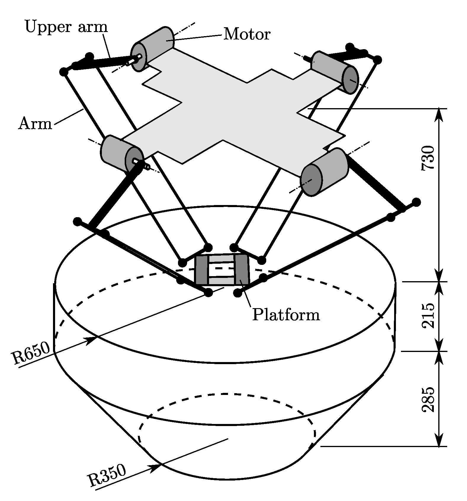
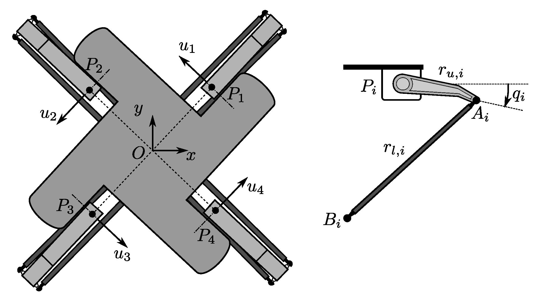
2. Model of the 4-DOF Parallel Robot
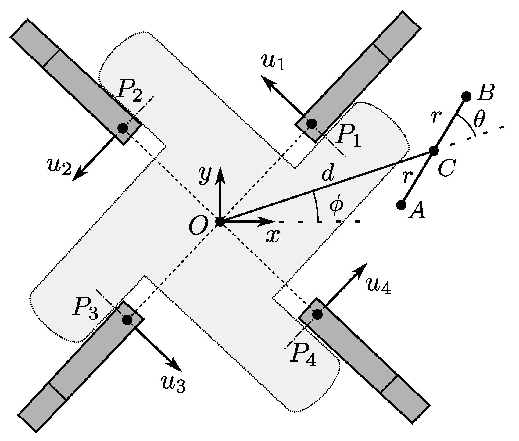
2.1. Kinematics
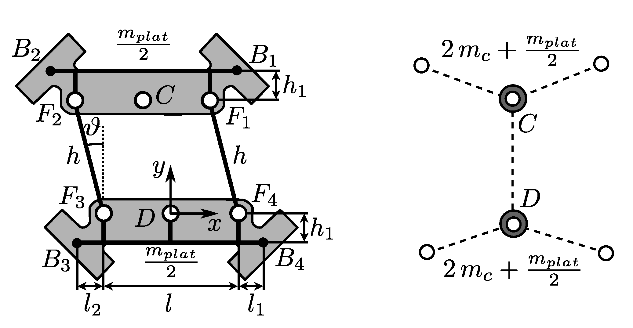
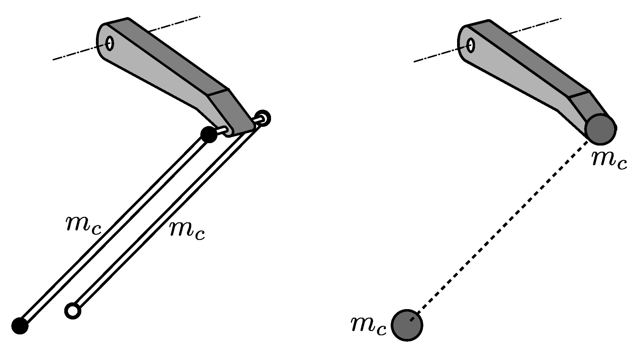
2.2. Dynamics
3. Electro-Mechanical Model
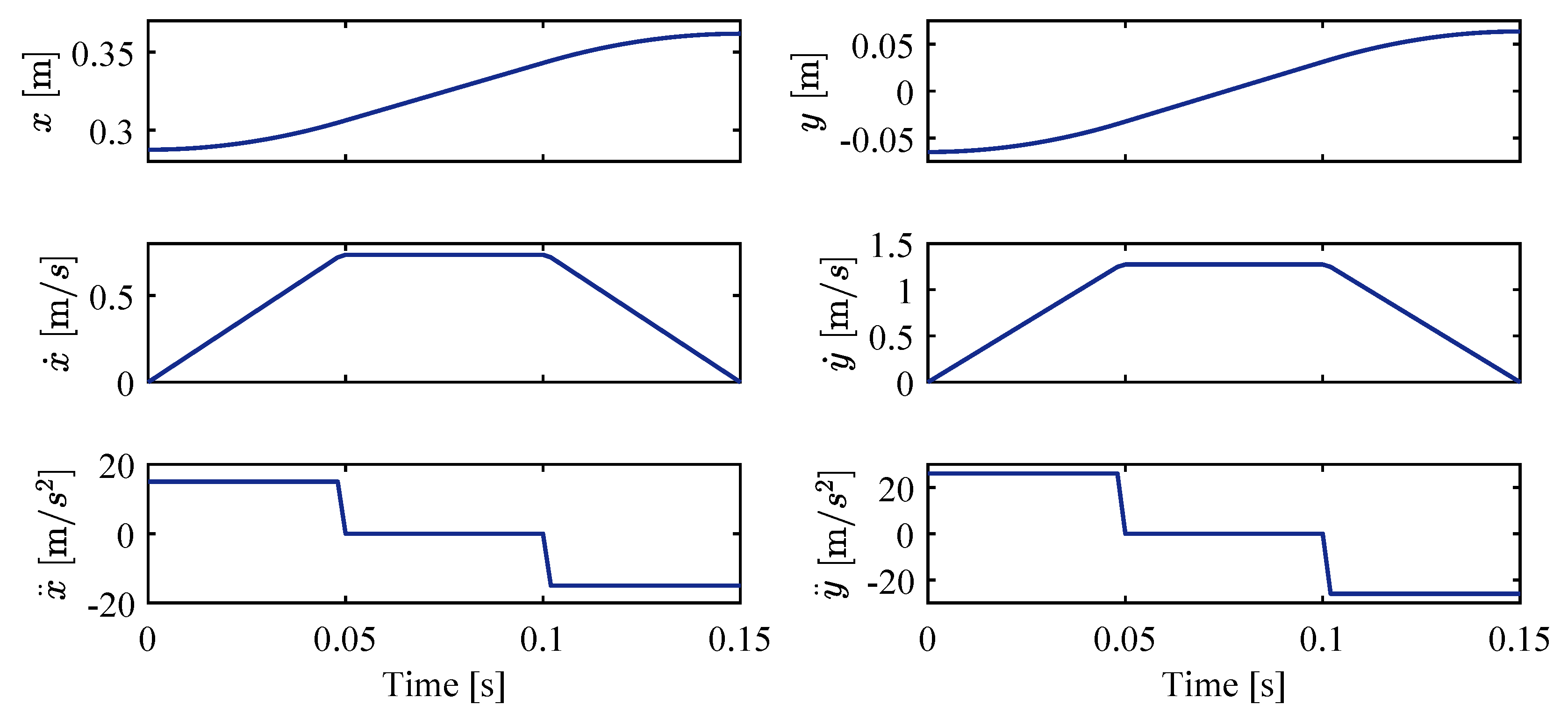
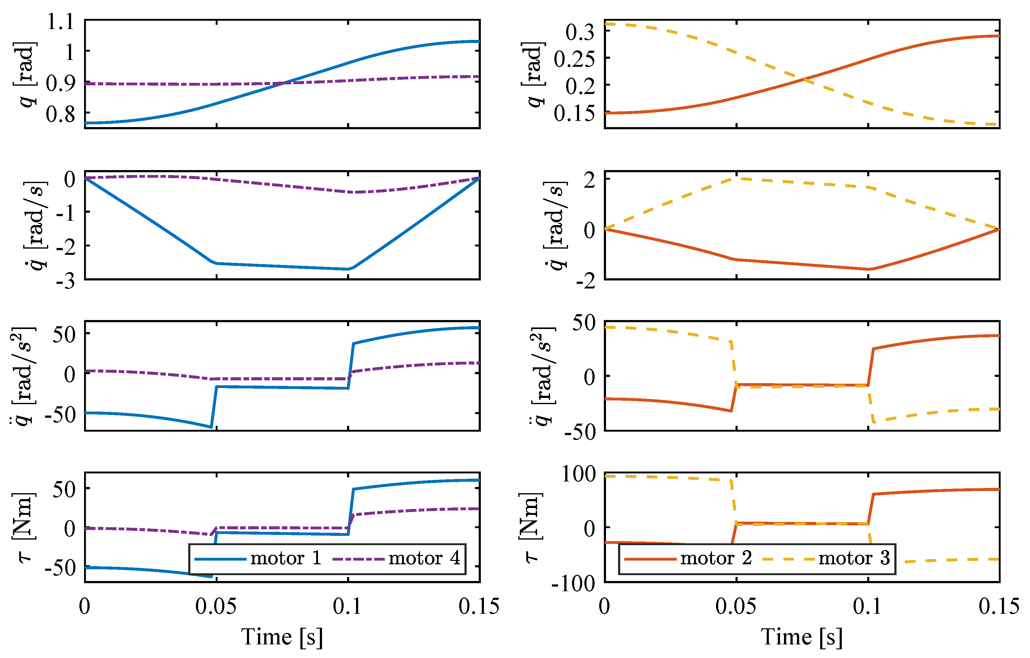
4. Task-Dependent Analysis
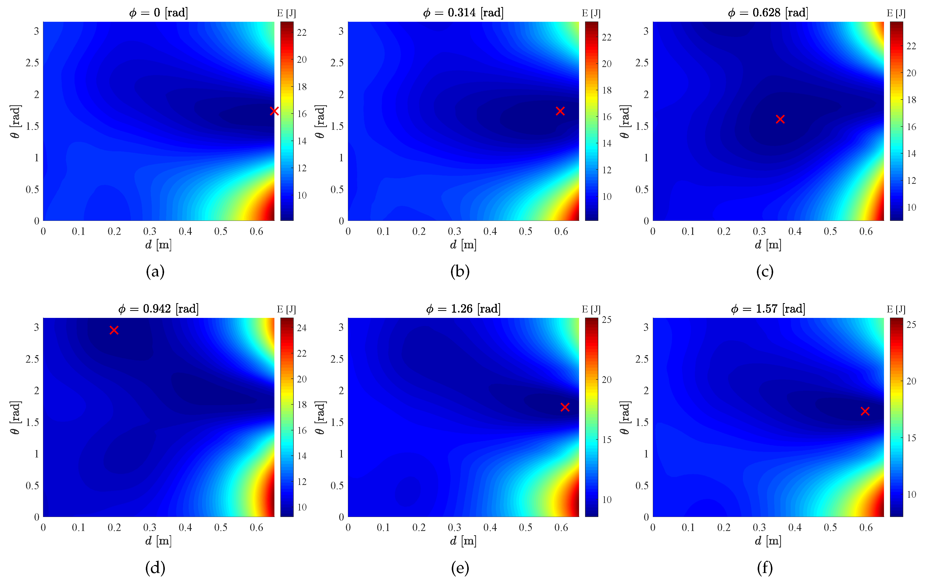
5. Results
6. Conclusions
Author Contributions
Funding
Conflicts of Interest
References
- European Comission. Proposal for a Directive of the European Parliament and of the Council Amending Directive 2012/27/EU on Energy Efficiency. Available online: https://eur-lex.europa.eu/homepage.html (accessed on 14 January 2020).
- Helm, D. The European framework for energy and climate policies. Energy Policy 2014, 64, 29–35. [Google Scholar] [CrossRef]
- Kucukvar, M.; Cansev, B.; Egilmez, G.; Onat, N.C.; Samadi, H. Energy-climate-manufacturing nexus: New insights from the regional and global supply chains of manufacturing industries. Appl. Energy 2016, 184, 889–904. [Google Scholar] [CrossRef] [Green Version]
- International Federation of Robotics. Executive Summary World Robotics 2019 Industrial Robots. Available online: https://ifr.org/free-downloads/ (accessed on 14 January 2020).
- Carabin, G.; Wehrle, E.; Vidoni, R. A review on energy-saving optimization methods for robotic and automatic systems. Robotics 2017, 6, 39. [Google Scholar] [CrossRef] [Green Version]
- Li, Y.; Bone, G.M. Are Parallel Manipulators More Energy Efficient? In Proceedings of the 2001 IEEE International Symposium on Computational Intelligence in Robotics and Automation (Cat. No. 01EX515), Banff, AB, Canada, 29 July–1 August 2001; pp. 41–46. [Google Scholar]
- Kim, Y.J. Design of Low Inertia Manipulator with HighStiffness and Strength using Tension Amplifying Mechanisms. In Proceedings of the IEEE/RSJ International Conference on Intelligent Robots and Systems (IROS), Hamburg, Germany, 28 September–2 October 2015; pp. 5850–5856. [Google Scholar]
- Boscariol, P.; Gallina, P.; Gasparetto, A.; Giovagnoni, M.; Scalera, L.; Vidoni, R. Evolution of a Dynamic Model for Flexible Multibody Systems. In Advances in Italian Mechanism Science; Springer: Basel, Switzerland, 2017; pp. 533–541. [Google Scholar]
- Yin, H.; Liu, J.; Yang, F. Hybrid structure design of lightweight robotic arms based on carbon fiber reinforced plastic and aluminum alloy. IEEE Access 2019, 7, 64932–64945. [Google Scholar] [CrossRef]
- Vidoni, R.; Scalera, L.; Gasparetto, A. 3-D ERLS based dynamic formulation for flexible-link robots: theoretical and numerical comparison between the finite element method and the component mode synthesis approaches. Int. J. Mech. Control 2018, 19, 39–50. [Google Scholar]
- Ghorbanpour, A.; Richter, H. Control With Optimal Energy Regeneration in Robot Manipulators Driven by Brushless DC Motors. In Proceedings of the ASME Dynamic Systems and Control Conference, Atlanta, GA, USA, 30 September–3 October 2018; p. V001T04A003. [Google Scholar]
- Carabin, G.; Palomba, I.; Wehrle, E.; Vidoni, R. Energy Expenditure Minimization for a Delta-2 Robot Through a Mixed Approach. In Proceedings of the IFToMM World Congress on Mechanism and Machine Science, Krakow, Poland, 30 June–4 July 2019; pp. 383–390. [Google Scholar]
- Khalaf, P.; Richter, H. Trajectory optimization of robots with regenerative drive systems: Numerical and experimental results. IEEE Trans. Robot. 2019. [Google Scholar] [CrossRef]
- Scalera, L.; Palomba, I.; Wehrle, E.; Gasparetto, A.; Vidoni, R. Natural motion for energy saving in robotic and mechatronic systems. Appl. Sci. 2019, 9, 3516. [Google Scholar] [CrossRef] [Green Version]
- Barreto, J.P.; Corves, B. Resonant Delta Robot for Pick-and-Place Operations. In Proceedings of the IFToMM World Congress on Mechanism and Machine Science, Krakow, Poland, 30 June–4 July 2019; pp. 2309–2318. [Google Scholar]
- Scalera, L.; Carabin, G.; Vidoni, R.; Wongratanaphisan, T. Energy efficiency in a 4-DOF parallel robot featuring compliant elements. Int. J. Mech. Control 2019, 20, 49–57. [Google Scholar]
- Paes, K.; Dewulf, W.; Vander Elst, K.; Kellens, K.; Slaets, P. Energy efficient trajectories for an industrial ABB robot. Proc. Cirp 2014, 15, 105–110. [Google Scholar] [CrossRef] [Green Version]
- Ho, P.M.; Uchiyama, N.; Sano, S.; Honda, Y.; Kato, A.; Yonezawa, T. Simple motion trajectory generation for energy saving of industrial machines. SICE J. Control Meas. Syst. Integr. 2014, 7, 29–34. [Google Scholar] [CrossRef] [Green Version]
- Boscariol, P.; Gasparetto, A.; Vidoni, R. Planning Continuous-Jerk Trajectories for Industrial Manipulators. In Proceedings of the ASME 2012 11th Biennial Conference on Engineering Systems Design and Analysis, Nantes, France, 2–4 July 2012; pp. 127–136. [Google Scholar]
- Boscariol, P.; Carabin, G.; Gasparetto, A.; Lever, N.; Vidoni, R. Energy-efficient point-to-point trajectory generation for industrial robotic machines. In Proceedings of the ECCOMAS Thematic Conference on Multibody Dynamics, Barcelona, Spain, 29 June–2 July 2015; pp. 1425–1433. [Google Scholar]
- Carabin, G.; Vidoni, R.; Wehrle, E. Energy Saving in Mechatronic Systems Through Optimal Point-to-Point Trajectory Generation Via Standard Primitives. In Proceedings of the International Conference of IFToMM ITALY, Cassino, Italy, 29–30 November 2018; pp. 20–28. [Google Scholar]
- Ruiz, A.G.; Fontes, J.V.; da Silva, M.M. The Influence of Kinematic Redundancies in the Energy Efficiency of Planar Parallel Manipulators. In Proceedings of the ASME 2015 International Mechanical Engineering Congress and Exposition, Houston, TX, USA, 13–19 November 2015; p. V04AT04A010. [Google Scholar]
- Boscariol, P.; Richiedei, D. Trajectory Design for Energy Savings in Redundant Robotic Cells. Robotics 2019, 8, 15. [Google Scholar] [CrossRef] [Green Version]
- Shiller, Z. Time-Energy Optimal Control of Articulated Systems with Geometric Path Constraints. In Proceedings of the 1994 IEEE International Conference on Robotics and Automation, San Diego, CA, USA, 8–13 May 1994; pp. 2680–2685. [Google Scholar]
- Trigatti, G.; Boscariol, P.; Scalera, L.; Pillan, D.; Gasparetto, A. A new path-constrained trajectory planning strategy for spray painting robots-rev.1. Int. J. Adv. Manuf. Technol. 2018, 98, 2287–2296. [Google Scholar] [CrossRef]
- Trigatti, G.; Boscariol, P.; Scalera, L.; Pillan, D.; Gasparetto, A. A Look-Ahead Trajectory Planning Algorithm for Spray Painting Robots with Non-Spherical Wrists. In Proceedings of the IFToMM Symposium on Mechanism Design for Robotics, Udine, Italy, 11–13 September 2018; pp. 235–242. [Google Scholar]
- Kalawoun, R.; Lengagne, S.; Mezouar, Y. Optimal Robot Base Placements for Coverage Tasks. In Proceedings of the IEEE 14th International Conference on Automation Science and Engineering (CASE), Munich, Germany, 20–24 August 2018; pp. 235–240. [Google Scholar]
- Scalera, L.; Seriani, S.; Gasparetto, A.; Gallina, P. Watercolour robotic painting: a novel automatic system for artistic rendering. J. Intell. Robot. Syst. 2019, 95, 871–886. [Google Scholar] [CrossRef]
- Scalera, L.; Mazzon, E.; Gallina, P.; Gasparetto, A. Airbrush Robotic Painting System: Experimental Validation of a Colour Spray Model. In Proceedings of the International Conference on Robotics in Alpe-Adria Danube Region, Turin, Italy, 21–23 June 2017; pp. 549–556. [Google Scholar]
- Boschetti, G. A picking strategy for circular conveyor tracking. J. Int. Robtic Syst. 2016, 81, 241–255. [Google Scholar] [CrossRef]
- Boscariol, P.; Scalera, L.; Gasparetto, A. Task-Dependent Energetic Analysis of a 3 dof Industrial Manipulator. In Proceedings of the International Conference on Robotics in Alpe-Adria Danube Region, Kaiserslautern, Germany, 19–21 June 2019; pp. 162–169. [Google Scholar]
- Patel, S.; Sobh, T. Manipulator performance measures-a comprehensive literature survey. J. Int. Robtic Syst. 2015, 77, 547–570. [Google Scholar] [CrossRef] [Green Version]
- Valsamos, C.; Wolniakowski, A.; Miatliuk, K.; Moulianitis, V.C. Optimal placement of a kinematic robotic task for the minimization of required joint velocities. Int. J. Mech. Control 2019, 20, 3–14. [Google Scholar]
- Tanev, T.; Stoyanov, B. On the performance indexes for robot manipulators. Probl. Eng. Cybern. Robot. 2000, 49, 64–71. [Google Scholar]
- Ur-Rehman, R.; Caro, S.; Chablat, D.; Wenger, P. Multi-objective path placement optimization of parallel kinematics machines based on energy consumption, shaking forces and maximum actuator torques: Application to the Orthoglide. Mech. Mach. Theory 2010, 45, 1125–1141. [Google Scholar] [CrossRef] [Green Version]
- Boschetti, G.; Rosa, R.; Trevisani, A. Optimal robot positioning using task-dependent and direction-selective performance indexes: General definitions and application to a parallel robot. Robot. Comput. Integr. Manuf. 2013, 29, 431–443. [Google Scholar] [CrossRef]
- Pierrot, F.; Nabat, V.; Company, O.; Krut, S.; Poignet, P. Optimal design of a 4-DOF parallel manipulator: From academia to industry. IEEE Trans. Robot. 2009, 25, 213–224. [Google Scholar] [CrossRef]
- Vidussi, F.; Boscariol, P.; Scalera, L.; Gasparetto, A. Energetic Analysis of Industrial Robots for Pick-and-Place Operations. In Proceedings of the 25th Jc-IFToMM Symposium (2019), 2nd Internationl Jc-IFToMM Symposium, Kanagawa, Japan, 26 October 2019. [Google Scholar]
- Sayed-Ahmed, A.; Wei, L.; Seibel, B. Industrial Regenerative Motor-Drive Systems. In Proceedings of the 2012 Twenty-Seventh Annual IEEE Applied Power Electronics Conference and Exposition (APEC), Orlando, FL, USA, 5–9 February 2012; pp. 1555–1561. [Google Scholar]


| Parameter | Value | Parameter | Value |
|---|---|---|---|
| l | |||
| h | |||
| Parameter | Symbol | Value | Parameter | Symbol | Value |
|---|---|---|---|---|---|
| motor torque constant | reduction ratio | 50 | |||
| motor back-emf constant | gearbox inertia | ||||
| winding resistance | R | upper arm mass | |||
| motor inertia | point mass (arm) | ||||
| static friction coefficient | platform mass | ||||
| viscous friction coefficient | load mass | ||||
| driver efficiency | load inertia | ||||
| gravitational acceleration | g | point mass (platform) |
| Case | |||||
|---|---|---|---|---|---|
| (1) | −0.80 | 0.150 | |||
| (2) | 0.00 | 0.150 | |||
| (3) | 0.00 | 0.00 | 0.350 |
| map | En. red. | |||||||
|---|---|---|---|---|---|---|---|---|
| (a) | 0.000 | 0.650 | 1.73 | 8.11 | 0.650 | 0.000 | 22.8 | 64.4 |
| (b) | 0.314 | 0.597 | 1.73 | 8.16 | 0.650 | 0.000 | 23.1 | 64.7 |
| (c) | 0.628 | 0.358 | 1.60 | 9.00 | 0.650 | 0.000 | 23.8 | 62.2 |
| (d) | 0.942 | 0.199 | 2.95 | 9.24 | 0.650 | 0.257 | 24.7 | 62.7 |
| (e) | 1.26 | 0.610 | 1.73 | 8.56 | 0.650 | 0.192 | 25.1 | 65.9 |
| (f) | 1.57 | 0.597 | 1.67 | 8.01 | 0.650 | 0.064 | 25.6 | 68.7 |
| Map | En. red. | |||||||
|---|---|---|---|---|---|---|---|---|
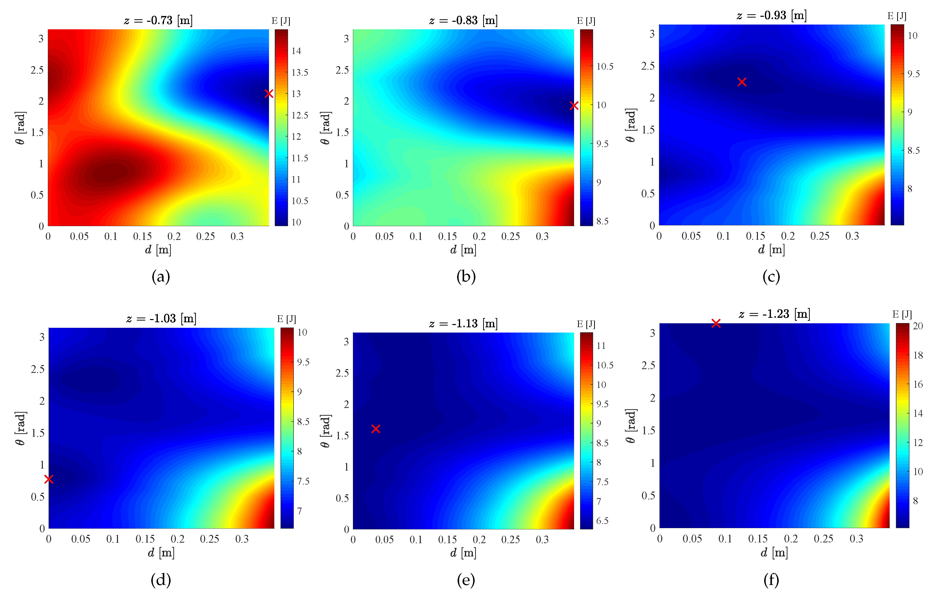
| (a) | −0.73 | 0.350 | 2.12 | 9.91 | 0.100 | 0.834 | 14.5 | 31.7 |
| (b) | −0.83 | 0.350 | 1.92 | 8.43 | 0.350 | 0.000 | 11.0 | 23.1 |
| (c) | −0.93 | 0.129 | 2.24 | 7.52 | 0.350 | 0.000 | 10.1 | 25.8 |
| (d) | −1.03 | 0.000 | 0.77 | 6.70 | 0.350 | 0.000 | 10.1 | 33.4 |
| (e) | −1.13 | 0.036 | 1.60 | 6.28 | 0.350 | 0.000 | 11.3 | 44.6 |
| (f) | −1.23 | 0.086 | 3.14 | 6.12 | 0.350 | 0.000 | 20.2 | 69.6 |
| En. red. | ||||||
|---|---|---|---|---|---|---|
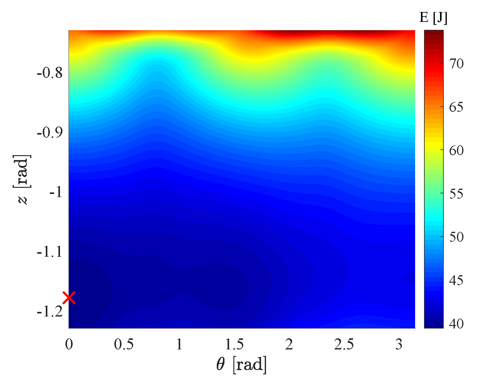
| −1.18 | 0.000 | 39.4 | −0.730 | 2.05 | 73.8 | 46.6 |
© 2020 by the authors. Licensee MDPI, Basel, Switzerland. This article is an open access article distributed under the terms and conditions of the Creative Commons Attribution (CC BY) license (http://creativecommons.org/licenses/by/4.0/).
Share and Cite
Scalera, L.; Boscariol, P.; Carabin, G.; Vidoni, R.; Gasparetto, A. Enhancing Energy Efficiency of a 4-DOF Parallel Robot Through Task-Related Analysis. Machines 2020, 8, 10. https://doi.org/10.3390/machines8010010
Scalera L, Boscariol P, Carabin G, Vidoni R, Gasparetto A. Enhancing Energy Efficiency of a 4-DOF Parallel Robot Through Task-Related Analysis. Machines. 2020; 8(1):10. https://doi.org/10.3390/machines8010010
Chicago/Turabian StyleScalera, Lorenzo, Paolo Boscariol, Giovanni Carabin, Renato Vidoni, and Alessandro Gasparetto. 2020. "Enhancing Energy Efficiency of a 4-DOF Parallel Robot Through Task-Related Analysis" Machines 8, no. 1: 10. https://doi.org/10.3390/machines8010010