A New Stiffness Performance Index: Volumetric Isotropy Index

Abstract

A new index for a precise calculation of a manipulator’s stiffness isotropy is introduced. The proposed index is compared with the conventionally used stiffness isotropy index by making use of the investigation on R-CUBE manipulator. The proposed index is shown to produce relatively more precise results from which a higher number of isotropic poses are detected.

1. Introduction

In industrial robotics, stiffness property has great importance especially when they are used in manufacturing processes. Production quality during milling and drilling operations depends on the stiffness performance of the robot. Thus, many academic studies are devoted to the stiffness analysis and evaluation of industrial robots [1,2,3,4,5,6,7].

One reason for the stiffness performance evaluation of a manipulator is to determine the capabilities of manipulators [4,8,9,10,11]. There are several evaluation approaches of stiffness properties. One is commonly used in industrial robots that consider the absolute end-effector deflection. In this approach, a specific position or a trajectory is given to the robot, and its positioning error is observed under external wrenches [8,12,13]. The procedures of this kind of evaluation are given in ANSI and ISO standards [4,14]. These methods are suitable to have a general idea on stiffness performance, but they may not distinguish whether forces or moments cause the elastic translational or rotational displacements. Depending on the performance output, a suitable manipulator for the desired task can be selected.

Another reason is to optimally design the manipulator parameters by considering the stiffness performance [5,6,7,13,15,16,17]. The optimal design process of a manipulator requires objective functions that include the stiffness performance indices. These indices are mainly used to achieve high rigidity while preserving low inertia and high kinematic performance.

In parallel robots, stiffness modulation can be achieved by introducing redundancy in actuation [18,19] and/or kinematics [20,21,22]. Stiffness characteristics of the manipulator are regulated by applying suitable redundancy resolution algorithms in control [19,20,21,23,24]. A common way of redundancy resolution is via null-space control [25] in which a performance index is designed. This performance index is defined as a stiffness performance index when it is required to modulate the stiffness of the manipulator [18,19,20,21,22,23,24]. A key aspect of this performance index is that it should be computationally efficient.

Optimal design and control processes require a mathematical stiffness model (stiffness matrix) of the manipulator to use the stiffness performance indices. These indices adopt common matrix operations such as the determinant, norm, or singular value decomposition (SVD) in defining the performance indices [3,4,5,6,8,9,10,11,13,14,16,17,26,27,28,29,30,31,32,33,34,35]. Each of them investigates a different property of the stiffness matrix. For instance, the determinant is accepted as a scalar indication of stiffness magnitude [3,11,14,16,26,28]. SVD computes the eigenvectors and eigenvalues that show the most/least stiff directions and their magnitudes [3,4,6,8,9,11,13,14,17,26,27,28,30]. Once the stiffness model is known these approaches are quite handy and they provide detailed stiffness information of the manipulator. However, their general problems are that they are calculated locally.

Isotropy is having the same stiffness performance distribution in all directions. In the literature, eigenvalues of the stiffness matrix are used for relative stiffness resolution evaluation. The evaluation is carried out by calculating the ratio of the maximum to the minimum eigenvalue. The index is named as stiffness condition number, stiffness dexterity, or stiffness isotropy index [10,13,14]. It obtains a directional stiffness resolution compared to the maximum eigenvalue. However, only focusing on maximum and minimum eigenvalues hides the effect of intermediate eigenvalues on the performance. For instance, there exist four possible cases for the distribution of eigenvalues of a 3 × 3 stiffness matrix.The first case is the one that has all different eigenvalues. The second case has two equal minimum eigenvalues. The third case has two equal maximum eigenvalues. The fourth case has all equal eigenvalues. For the first three cases, if the minimum and maximum eigenvalues are the same, then, the stiffness isotropy index computation will output the same value. However, it is clear that the isotropy of first, second, and third cases should be different from each other. This problem can only be resolved by taking into account the intermediate eigenvalues in stiffness isotropy computation.

In this study, special attention is directed towards this intermediate eigenvalue problem. In this regard, a new performance index is proposed. This index composes a volumetric isotropy index by considering intermediate eigenvalues. As a case study, an R-CUBE [36] parallel manipulator is considered. A comparison is conducted between the proposed volumetric isotropy index and existing isotropy index. R-CUBE is selected for this analysis since it has relatively trivial kinematics to be in conveniently used in the formulation of its stiffness model [36].

The remaining sections of this paper are organized as follows; in Section 2 stiffness model of the R-CUBE is obtained, and notations are given. Then, in Section 3, currently used performance indices are discussed, and a new performance index is introduced. In Section 4, results of conventional isotropy index and the new index computations are presented. Finally, conclusions are stated in Section 5.

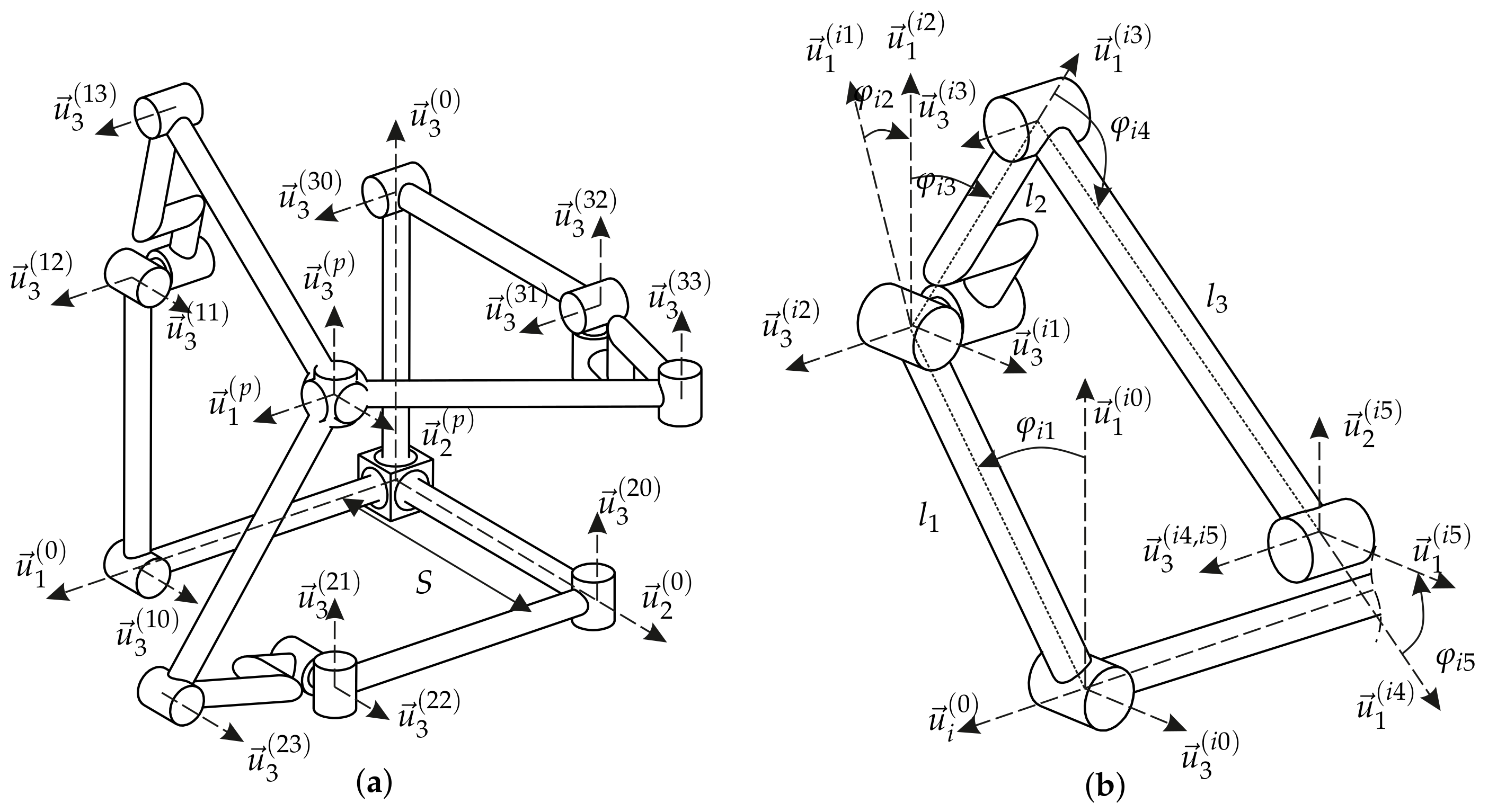
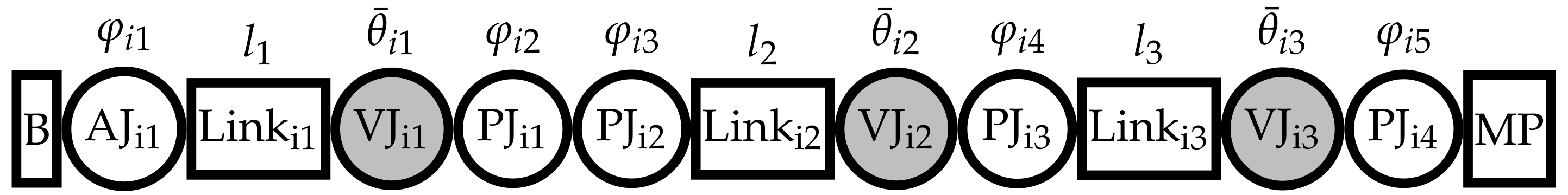
2. Stiffness Model of R-CUBE

The R-CUBE manipulator is introduced by [36]. The manipulator composed of revolute joints, only. In total, 3 serial chains exist, and each one of them controls their respective translational DoF in Cartesian space. In Figure 1 the kinematic model is illustrated.

In Figure 1a, first refecence frames of the each serial chain are located on ${\overrightarrow{u}}_k^{(0)}$ orthogonal axes along kth axis for $k=1,2,3$. $ij$ stands for the jth frame in ith serial chain as shown in Figure 1b. ${\overrightarrow{u}}_k^{(0)}\Vert {\overrightarrow{u}}_k^{(p)}$ due the kinematic constraints. p is mobile platform frame. Besides, ${\overrightarrow{u}}_3^{(15)},{\overrightarrow{u}}_3^{(25)},{\overrightarrow{u}}_3^{(35)}$ are always aligned with ${\overrightarrow{u}}_1^{(35)},{\overrightarrow{u}}_1^{(15)},{\overrightarrow{u}}_1^{(25)}$ vectors, respectively. The forward kinematics is given as:

$$\begin{array}{cc}\hfill r_i& =S+l_{1}sin{\phi }_{i1}\mathrm{for}i=1,2,3\mathrm{and}\overline{r}={\left[\begin{array}{ccc}{r}_1& r_2& r_3\end{array}\right]}^T\hfill \end{array}$$

(1)

where S is a constant distance from 0th frame to ${\overrightarrow{u}}_3^{(i0)}$ frame. $\overline{r}$ denotes position vector with respect to the origin.

Commonly used stiffness (elasto-static) modeling methods are classified as Finite Element Method (FEM) [37,38], Matrix Structural Method (MSM) [39,40], and Virtual Joint Method (VJM) [28,41,42,43,44,45]. FEM exhibits the highest accuracy in exchange of computation cost due to its numerical approach. Besides, a meshing operation must be conducted for each pose of the manipulator. VJM and MSM are faster in this evaluation since they construct semi-analytical or analytical models. Thus, stiffness performance metrics are used via VJM and MSM for evaluation of a manipulator in any of its pose. In this study, VJM approach is adopted.

Stiffness model of the R-CUBE manipulator is computed by combining the stiffness models of each serial chain. Compliance model of ith serial chain and its connection to base and mobile platforms are illustrated in Figure 2. Passive and active joints have 1 degree-of-freedom (DoF) while virtual joints have 6 DoF (3 translations + 3 rotations). A virtual joint is defined as:

$${\mathit{H}}_v({\overline{\theta }}_{ij})={\mathit{T}}_1({\theta }_{ij}^1){\mathit{T}}_2({\theta }_{ij}^2){\mathit{T}}_3({\theta }_{ij}^3){\mathit{R}}_1({\theta }_{ij}^4){\mathit{R}}_2({\theta }_{ij}^5){\mathit{R}}_3({\theta }_{ij}^6)$$

(2)

where ${\mathit{H}}_v$ denotes the homogeneous transformation matrix (HTM). ${\mathit{T}}_k$ and ${\mathit{R}}_k$ are pure translational HTM along and pure rotational HTM about ${\overrightarrow{u}}_k$th axis for $k=1,2,3$. ${\overline{\theta }}_{ij}$ is a vector that contains virtual joint variables. Superscripts of ${\theta }_{ij}$ represents the element number.

The compliant kinematic model is computed as follows:

$$\begin{array}{c}\hfill \begin{array}{cc}\hfill {\mathit{H}}^{(i0,K_{i1})}& ={\mathit{R}}_3({\phi }_{i1}){\mathit{T}}_{1u}(l_1){\mathit{H}}_v({\overline{\theta }}_{i1})\hfill \\ \hfill {\mathit{H}}^{(K_{i1},K_{i2})}& ={\mathit{R}}_3({\phi }_{i2}){\mathit{R}}_1(-\pi /2){\mathit{R}}_3({\phi }_{i3}){\mathit{T}}_1(l_2){\mathit{H}}_v({\overline{\theta }}_{i2})\hfill \\ \hfill {\mathit{H}}^{(K_{i2},K_{i3})}& ={\mathit{R}}_3({\phi }_{i4}){\mathit{T}}_1(l_3){\mathit{H}}_v({\overline{\theta }}_{i3})\hfill \\ \hfill {\mathit{H}}^{(K_{i3},i5)}& ={\mathit{R}}_3({\phi }_{i5})\hfill \\ \hfill {\mathit{H}}_{Ki}& ={\mathit{H}}^{(0,i0)}{\mathit{H}}^{(i0,K_{i1})}{\mathit{H}}^{(K_{i1},K_{i2})}{\mathit{H}}^{(K_{i2},K_{i3})}{\mathit{H}}^{(K_{i3},i5)}{\mathit{H}}^{(i5,p)}\hfill \\ \hfill {\mathit{H}}_{Ki}& =\left[\begin{array}{cc}{\mathit{R}}_{Ki}& {\overline{r}}_{Ki}\\ {\overline{0}}^T& 1\end{array}\right]\hfill \end{array}\end{array}$$

(3)

where ${\mathit{H}}_{Ki}$ is the compliant transformation matrix of the ith serial kinematic chain of R-CUBE, and ${\mathit{H}}_{K1}={\mathit{H}}_{K2}={\mathit{H}}_{K3}$ by the assumption of a rigid mobile platform.

Active joints are assumed to be rigidly locked to exclude actuation stiffness in the structural stiffness calculations. Then, virtual and passive joint variables are arranged in a matrix form as follows:

$$\begin{array}{c}\hfill \begin{array}{cc}\hfill {\overline{q}}_{pi}& ={\left[\begin{array}{cccc}{\phi }_{i2}& {\phi }_{i3}& {\phi }_{i4}& {\phi }_{i5}\end{array}\right]}_{4\times 1}^T, {\overline{\theta }}_i={\left[\begin{array}{ccc}{\overline{\theta }}_{i1}^T& {\overline{\theta }}_{i2}^T& {\overline{\theta }}_{i3}^T\end{array}\right]}_{18\times 1}^T, {\overline{Q}}_i={\left[\begin{array}{cc}{\overline{\theta }}_i^T& {\overline{q}}_{pi}^T\end{array}\right]}_{22\times 1}^T\hfill \end{array}\end{array}$$

(4)

where ${\overline{q}}_{pi}$ denotes passive joint variables, ${\overline{Q}}_i$ is generalized coordinates of ith serial chain. ${\overline{Q}}_i$ is used to obtain Jacobian matrices as follows:

$$\begin{array}{cc}\hfill \frac{\partial {\mathit{H}}_{Ki}}{\partial Q_{ik}}& =\left[\begin{array}{cc}\frac{\partial {\mathit{R}}_{Ki}}{\partial Q_{ik}}& \frac{\partial {\overline{r}}_{Ki}}{\partial Q_{ik}}\\ {\overline{0}}^T& 1\end{array}\right] \mathrm{for} =k=1,2,\dots ,22\hfill \end{array}$$

(5)

where subscript k denotes the kth variable of $\overline{Q_i}$.

The Jacobian matrix ${\mathit{J}}_{Ki}$ for passive and virtual joints is given as follows:

$$\begin{array}{cc}\hfill {\mathit{J}}_{Ki}& ={\left[\begin{array}{cccc}{\overline{J}}_{Ki1}& {\overline{J}}_{Ki2}& \dots & {\overline{J}}_{Ki22}\end{array}\right]}_{6\times 22}\hfill \end{array}$$

(6)

where ${\overline{J}}_{Kik}$ for $k=1,2,\dots ,22$ denotes the Jacobian column matrices that are related with k th variable of $Q_i$.

${\mathit{J}}_{Ki}$ can be divided into sub-matrices as ${\mathit{J}}_{\theta i}$ and ${\mathit{J}}_{pi}$. They denote Jacobian matrices of virtual and passive joints. Sub-matrices are presented as follows:

$$\begin{array}{c}\hfill \begin{array}{cc}\hfill {\mathit{J}}_{\theta i}& ={\left[\begin{array}{cccc}{\overline{J}}_{Ki1}& {\overline{J}}_{Ki2}& \dots & {\overline{J}}_{Ki18}\end{array}\right]}_{6\times 18}\hfill \\ \hfill {\mathit{J}}_{pi}& ={\left[\begin{array}{cccc}{\overline{J}}_{Ki19}& {\overline{J}}_{Ki20}& {\overline{J}}_{Ki21}& {\overline{J}}_{Ki22}\end{array}\right]}_{6\times 4}\hfill \\ \hfill {\mathit{J}}_{Ki}& ={\left[\begin{array}{cc}{\mathit{J}}_{\theta i}& {\mathit{J}}_{pi}\end{array}\right]}_{6\times 22}\hfill \end{array}\end{array}$$

(7)

Note that, except in a kinematically singular configuration, ${\mathit{J}}_{\theta i}$ is always full-rank since the virtual joints have decoupled DoF. Similarly, ${\mathit{J}}_{pi}$ gets rank deficient in kinematic singularities.

Jacobian matrices relate small deflections of joints to task space variables:

$$\begin{array}{c}\hfill \begin{array}{cc}\hfill {\overline{X}}_i& =\overline{f}({\overline{Q}}_i), \Rightarrow \Delta {\overline{X}}_i={\mathit{J}}_{Ki}\Delta {\overline{Q}}_i\hfill \\ \hfill \Delta {\overline{X}}_i& ={\mathit{J}}_{\theta i}\Delta {\overline{\theta }}_i+{\mathit{J}}_{pi}\Delta {\overline{q}}_{pi}\hfill \end{array}\end{array}$$

(8)

where $\Delta {\overline{X}}_i$ is 6 × 1 column matrix of translational and rotational compliant deflections in task space that are calculated for the ith serial chain. $\Delta$ operator denotes the change between initial and final states. In the initial state, there is no applied wrench. In the final state, an external wrench is applied to the manipulator.

The relation between the external force/torque applied at the end-effector and joint space force/torque is provided via a property of Jacobian matrix that is given as follows:

$$\begin{array}{cc}\hfill {\overline{F}}_{Ki}& ={\mathit{J}}_{Ki}^T{\overline{F}}_{ext}\hfill \end{array}$$

(9)

where ${\left[{\overline{F}}_{Ki}\right]}_{22\times 1}$ is the joint space force/torque vector. ${\left[{\overline{F}}_{ext}\right]}_{6\times 1}$ is the external wrench. ${\overline{F}}_{Ki}$ is divided into sub-components and the force/torque vector on each joint are found as follows:

$$\begin{array}{c}\hfill \begin{array}{cc}\hfill {\overline{F}}_{Ki}& ={\left[\begin{array}{cc}{\overline{F}}_{\theta i}^T& {\overline{F}}_{pi}^T\end{array}\right]}^T\hfill \\ \hfill {\left[\begin{array}{cc}{\overline{F}}_{\theta i}^T& {\overline{F}}_{pi}^T\end{array}\right]}^T& ={\left[\begin{array}{cc}{\mathit{J}}_{\theta i}& \mathbf{0}\end{array}\right]}^T{\overline{F}}_{ext}+{\left[\begin{array}{cc}\mathbf{0}& {\mathit{J}}_{pi}\end{array}\right]}^T{\overline{F}}_{ext}\hfill \end{array}\end{array}$$

(10)

where ${\overline{F}}_{\theta i}$ and ${\overline{F}}_{pi}$ are force/torque vectors of virtual and passive joints.

${\overline{F}}_{Ki}$ is a function of the stiffness matrix and deflections that are defined in joints space.

$${\overline{F}}_{Ki}=\mathrm{diag}({\mathit{K}}_{\theta i},{\mathit{K}}_{pi})\Delta {\overline{Q}}_i \mathrm{and} {\mathit{K}}_{\theta i}=\mathrm{diag}({\mathit{K}}_{\theta i1},{\mathit{K}}_{\theta i2},{\mathit{K}}_{\theta i3})$$

(11)

where ${\mathit{K}}_{\theta ik}$ denotes stiffness matrix of kth link as expressed in [46] for a beam. Parameters of this stiffness matrix depends on the link geometry and material property. ${\mathit{K}}_{\theta i}$ denotes the stiffness matrix of ith serial chain. ${\mathit{K}}_{pi}$ denotes stiffness of passive joints. A relation is expressed in Cartesian space as follows:

$$\begin{array}{cc}\hfill {\mathit{J}}_{Ki}^T{\overline{F}}_{ext}& =\mathrm{diag}({\mathit{K}}_{\theta i},{\mathit{K}}_{pi})\Delta {\overline{Q}}_i \mathrm{and} {\mathit{J}}_{Ki}^{-1}\Delta {\overline{X}}_i=\Delta {\overline{Q}}_i\hfill \\ \hfill \Rightarrow {\overline{F}}_{ext}& =({\mathit{J}}_{\theta i}^{-T}{\mathit{K}}_{\theta i}{\mathit{J}}_{\theta i}^{-1}+{\mathit{J}}_{pi}^{-T}{\mathit{K}}_{pi}{\mathit{J}}_{pi}^{-1})\Delta {\overline{X}}_i\hfill \end{array}$$

(12)

Passive joints do not generate reaction torques about their rotation axes. Hence, ${\mathit{K}}_{pi}=\mathbf{0}$. Thus, ${\overline{F}}_{Ki}$ contains only force/torque of virtual joints. Hence:

$$\begin{array}{cc}\hfill {\overline{F}}_{ext}& =({\mathit{J}}_{\theta i}^{-T}{\mathit{K}}_{\theta i}{\mathit{J}}_{\theta i}^{-1})\Delta {\overline{X}}_i\hfill \\ \hfill {\mathit{J}}_{pi}^T{\overline{F}}_{ext}& =\overline{0}\hfill \end{array}$$

(13)

The effect of passive joints is included in the stiffness model by inverting the following homogeneous relation matrix. This matrix is always invertible if $det({\mathit{J}}_{\theta i}^T{\mathit{J}}_{\theta i})\ne 0$.

$$\begin{array}{cc}\hfill {\left[\begin{array}{cc}({\mathit{J}}_{\theta i}{\mathit{K}}_{\theta i}^{-1}{\mathit{J}}_{\theta i}^T)& {\mathit{J}}_{pi}\\ {\mathit{J}}_{pi}^T& \mathbf{0}\end{array}\right]}^{-1}& =\left[\begin{array}{cc}{\left[{\mathit{K}}_{Ci}\right]}_{6\times 6}& \sim \\ \sim & \sim \end{array}\right]\hfill \end{array}$$

(14)

where ${\mathit{K}}_{Ci}$ denotes stiffness matrix of ith in Cartesian space. Note that, ${\mathit{K}}_{Ci}$ is rank deficient due to the passive joints. Cartesian stiffness matrix of the manipulator, ${\mathit{K}}_C$, is computed as ${\mathit{K}}_C={\sum }_{i=1}^3{\mathit{K}}_{Ci}$. If external wrench is assumed to be ${\overline{F}}_{ext}=\overline{0}$, ${\mathit{K}}_C$ takes the following form.

$${\mathit{K}}_C=\left[\begin{array}{cccccc}{K}_{C_1}^{(11)}& 0& 0& 0& K_{C_1}^{(15)}& K_{C_1}^{(16)}\\ 0& K_{C_2}^{(22)}& 0& K_{C_2}^{(24)}& 0& K_{C_2}^{(26)}\\ 0& 0& K_{C_3}^{(33)}& K_{C_3}^{(34)}& K_{C_3}^{(35)}& 0\\ 0& K_{C_2}^{(24)}& K_{C_3}^{(34)}& K_{C_2}^{(44)}+K_{C_3}^{(44)}& K_{C_3}^{(45)}& K_{C_2}^{(46)}\\ K_{C_1}^{(15)}& 0& K_{C_3}^{(35)}& K_{C_3}^{(45)}& K_{C_1}^{(55)}+K_{C_3}^{(55)}& K_{C_1}^{(56)}\\ K_{C_1}^{(16)}& K_{C_2}^{(26)}& 0& K_{C_2}^{(46)}& K_{C_1}^{(56)}& K_{C_1}^{(66)}+K_{C_2}^{(66)}\end{array}\right]$$

(15)

For small deflections and loads, this matrix can be used without causing high errors. This matrix must be re-computed if $|{\overline{F}}_{ext}|>>0$. ${\mathit{K}}_C$ is divided into 33 sub-matrices.

$$\begin{array}{cc}\hfill {\mathit{K}}_C& =\left[\begin{array}{cc}{\mathit{K}}_A& {\mathit{K}}_B\\ {\mathit{K}}_B^T& {\mathit{K}}_D\end{array}\right]\hfill \end{array}$$

(16)

where ${\mathit{K}}_A$, ${\mathit{K}}_B$, ${\mathit{K}}_B^T$, and ${\mathit{K}}_D$ have the units of N/m, N/rad, N/rad, and Nm, respectively. The kinematic dimensions and material properties of the links are given in [47]. This study makes use of these parameters for stiffness evaluation of R-CUBE manipulator.

3. Stiffness Performance Indices

In this section, a review of the existing performance indices in literature is described, and a new performance index for isotropy evaluation of the stiffness matrix is proposed. Besides, usage of the indices for the R-CUBE manipulator is given in a table.

3.1. Performance Indices in the Literature

Stiffness performance indices are computed by obtaining the eigenvalues and eigenvectors. SVD operation may be used to obtain these properties as follows:

$$\begin{array}{cc}\hfill \mathit{K}& =\mathit{Q}\mathit{D}\mathit{U}\hfill \end{array}$$

(17)

where $\mathit{K}$ is an $n\times n$ stiffness matrix defined in Cartesian space for $n=1,2,\dots ,6$. $\mathit{Q}$ and $\mathit{U}$ are orthogonal matrices whose columns are the eigenvectors of $\mathit{K}$. Since $\mathit{K}$ is a symmetric matrix, $\mathit{Q}={\mathit{U}}^T$. $\mathit{D}$ is a diagonal matrix whose elements denote the positive eigenvalues. These matrices are shown as:

$$\begin{array}{cc}\hfill \mathit{Q}& =\left[\begin{array}{cccc}{\overline{e}}_1& {\overline{e}}_2& \dots & {\overline{e}}_6\end{array}\right]\hfill \end{array}$$

(18)

$$\begin{array}{cc}\hfill \mathit{D}& =diag({\lambda }_1,{\lambda }_2,\dots ,{\lambda }_6)\hfill \end{array}$$

(19)

$$\begin{array}{c}{\lambda }_1\le {\lambda }_2\le \dots \le {\lambda }_6\hfill \end{array}$$

(20)

where ${\overline{e}}_i$ and ${\lambda }_i$ for $i=1,2,\dots ,6$ denote the eigenvectors and eigenvalues, respectively. Regardless of the kinematic DoF of the manipulator, stiffness matrix is always a 6 × 6 matrix because compliant displacement may occur in any direction in 6 DoF space. Direct evaluation of a 6 × 6 stiffness matrix causes unit inconsistency in the results. A simple method is to use the normalized stiffness matrix [48]. The proposed method uses pre- and post-multiplication of the matrix with diagonal scaling matrices. Another method is introduced by Angeles [49]. He used the natural length to obtain normalized and unity matrix. Plücker Coordinates is preferred by Khan and Angeles to use dimensionally homogeneous space [50]. Thus, the dimensionally homogeneous matrix is obtained. A separate evaluation of rotation sensitive and translation sensitive matrices are introduced by Cardou et al. [51]. Hence, it is also possible to use interested sub-matrices of 6 × 6 stiffness matrix. In this way, a certain aspect of the stiffness model can be placed in focus. In our case, since we focus on the translational compliant displacements of the mobile platform, we used the top left corner of the stiffness matrix as indicated in Equation (16). Hence, in this sub-matrix, unit consistency is achieved. Nevertheless, this produces a lower dimensional stiffness matrix.

The graphical illustration of eigenvectors and eigenvalues generates an n-dimensional surface. This surface becomes a line for $n=1$, an ellipse for $n=2$, an ellipsoid for $n=3$, and a hyper-ellipsoid for $n=4,5,6$. The radii and axes of ellipsoids are defined by eigenvectors and eigenvalues as shown in Figure 3 for $n=3$ [26].

Eigenvalues indicate the magnitude of the stiffness along their respective eigenvectors. Hence, the volume of this ellipsoid indicates the stiffness capacity. This volume is proportional to the determinant of the stiffness matrix [3,11,14,16,26,27,28,32]. Thus, stiffness value is commonly computed as:

$$\begin{array}{cc}\hfill {\gamma }_V& =det(\mathit{K})=\prod _{i=1}^n{\lambda }_i\hfill \end{array}$$

(21)

where ${\gamma }_V$ denotes an average stiffness magnitude, and ${\lambda }_i$ is the ith eigenvalue. ${\gamma }_V$ equals to zero when inspected pose of the manipulator has at least one free motion direction. This case corresponds to a stiffness singularity. Thus, such a singular pose can be determined by investigating ${\gamma }_V$.

The Euclidean norm ${\Vert .\Vert }_E$, which is also named as 2-norm ${\Vert .\Vert }_2$, computes the square root of the largest positive eigenvalue (or singular value) of the square of a matrix, $\mathit{K}{\mathit{K}}^T$ shown as follows:

$$\begin{array}{cc}\hfill {\Vert \mathit{K}\Vert }_E& =max(\sqrt{{\tilde{\lambda }}_i})\hfill \end{array}$$

(22)

where ${\tilde{\lambda }}_i$ denotes the ith eigenvalue of matrix $\mathit{K}{\mathit{K}}^T$. This norm exhibits the maximum eigenvalue of $\mathit{K}$ which is also the largest radius of the ellipsoid. The direction of this eigenvalue is the direction of the displacement which exhibits the highest stiffness. Euclidean norm of ${\mathit{K}}^{-1}$ reveals the minimum eigenvalue of $\mathit{K}$, which indicates the most compliant direction [14,17,27,29,30,33]. In optimization problems, it is common to only focus on minimum eigenvalue in the workspace in order to maximize it.

Other norms are 1 norm ${\Vert .\Vert }_1$, infinity norm ${\Vert .\Vert }_{\infty }$ (also named as Chebyshev norm ${\Vert .\Vert }_C$), and Frobenius norm ${\Vert .\Vert }_F$. 1 norm computes the maximum of the summation of absolute values of column elements of a matrix. Infinity norm makes this computation for rows. Since the stiffness matrix is symmetric, both norms result in the same values. These norms denote a combined total resistive force and moment against a unit displacement in Cartesian space. Frobenius norm, on the other hand, has more meaning in terms of average stiffness. It focuses on diagonal elements of $\mathit{K}{\mathit{K}}^T$. It is computed as follows:

$$\begin{array}{cc}\hfill {\Vert \mathit{K}\Vert }_F& ={\left(\sum _{i=1}^n\sum _{j=1}^n{({\mathit{K}}_{ij})}^2\right)}^{1/2}=\sqrt{tr(\mathit{K}{\mathit{K}}^T)}=\sqrt{{\lambda }_1^2+{\lambda }_2^2+\dots +{\lambda }_n^2}\hfill \end{array}$$

(23)

where $tr$ is the trace operator and subscript $ij$ denotes the $ij$th element of the matrix. All norms result in higher values in stiff poses and lower values in compliant poses. Hence, they show similar relative distribution throughout the workspace. Therefore, an evaluation of one of the norms is sufficient to have an idea of stiffness distribution depending on manipulator pose.

Stiffness condition number, stiffness dexterity, or stiffness isotropy index is computed as the ratio of the maximum eigenvalue to the minimum eigenvalue [3,6,10,14,17,26,28,31]. This ratio reveals stiffness value distribution among eigenvectors. The minimum ratio of 1 indicates equal stiffness distribution. The calculation of this index is given as:

$$\begin{array}{cc}\hfill {\gamma }_C& =\frac{{\lambda }_n}{{\lambda }_1}={\Vert \mathit{K}\Vert }_E{\Vert {\mathit{K}}^{-1}\Vert }_E\hfill \end{array}$$

(24)

where ${\gamma }_C$ is stiffness condition number.

Another stiffness performance index is the uniformity index which compares the maximum and minimum values of ${\gamma }_C$. This index is formulated as follows:

$$\begin{array}{cc}\hfill {\gamma }_{CU}& =\frac{max({\gamma }_C)}{min({\gamma }_C)}\hfill \end{array}$$

(25)

$$\begin{array}{cc}\hfill {\gamma }_{CU}& \ge 1\hfill \end{array}$$

(26)

where ${\gamma }_{CU}$ is the uniformity index. Notice that, the minimum value of ${\gamma }_C$ is bounded by 1 and so ${\gamma }_{CU}\ge 1$. Here, ${\gamma }_{CU}=1$ can only be achieved when the maximum and minimum values of ${\gamma }_C$ are equal to each other. The only condition that satisfies this equality is when all ${\gamma }_C$ in all poses are equal to each other.

The determination of both stiff and isotropic poses is a problem. A solution is proposed in [15] that evaluates the stiffness magnitude and isotropy, simultaneously. The formulation of this index is given below.

$$\begin{array}{cc}\hfill {\gamma }_G& =\frac{{\lambda }_n^2{\lambda }_1^2}{{\lambda }_n+{\lambda }_1}\hfill \end{array}$$

(27)

${\gamma }_G$ value increases as the manipulator approaches a stiff and isotropic pose. This index is more suitable for 2 × 2 stiffness matrices. For higher dimensions, this approach is not appropriate because the problem turns into a volumetric problem while ${\gamma }_G$ solves a surface equation.

Energy index computation depends on whether a constant payload is applied or a constant compliant displacement is given to a manipulator. For a constant payload, stiff poses of the manipulator result in smaller deflections. Since the energy has a quadratic relationship with elastic displacements, stiff manipulators store less energy for the same payload. Therefore, the highest stored energy is observed when the elastic displacement is along the eigenvector direction that has the minimum eigenvalue for a payload. On the other hand, when a constant compliant displacement is given to manipulator, obviously stiff poses store more energy. It means the highest energy for a constant displacement is observed when this displacement is given along the eigenvector that has the highest eigenvalue. For a unit displacement, stored energy equals to the half of the maximum eigenvalue. The index formulation is given as:

$$\begin{array}{cc}\hfill {\gamma }_{ϵ}& =\frac{1}{2}\Delta {\overline{X}}^T\mathit{K}\Delta \overline{X} \Rightarrow {\gamma }_{ϵ}=\frac{1}{2}{\overline{e}}_n^T\mathit{K}{\overline{e}}_n \Rightarrow {\gamma }_{ϵ}=\frac{1}{2}{\lambda }_n \Rightarrow {\gamma }_{ϵ}=\frac{1}{2}{\Vert \mathit{K}\Vert }_E\hfill \end{array}$$

(28)

where ${\gamma }_{ϵ}$ is the energy index [5,7,11,52].

Unfortunately, all the above indices are computed numerically. In addition, they are local indices (except ${\gamma }_{CU}$). Hence, they are pose dependent, and they only indicate local performances. Thus, a globalization process is necessary for these indices [35]. This globalization can be achieved for the abovementioned indices to obtain an average value of performance of the whole workspace as follows:

$$\begin{array}{cc}\hfill \overline{\mu }& =\frac{\int \mu dv}{\int dv}\hfill \end{array}$$

(29)

$$\begin{array}{cc}\hfill \sigma & =\sqrt{\frac{\int {(\mu -\overline{\mu })}^{2}dv}{\int dv}}\hfill \end{array}$$

(30)

where $\mu$ denotes any of the performance indices. $\overline{\mu }$ is an average value, and $\sigma$ is the standard deviation. It is desired to have a low deviation to have a uniform stiffness performance distribution.

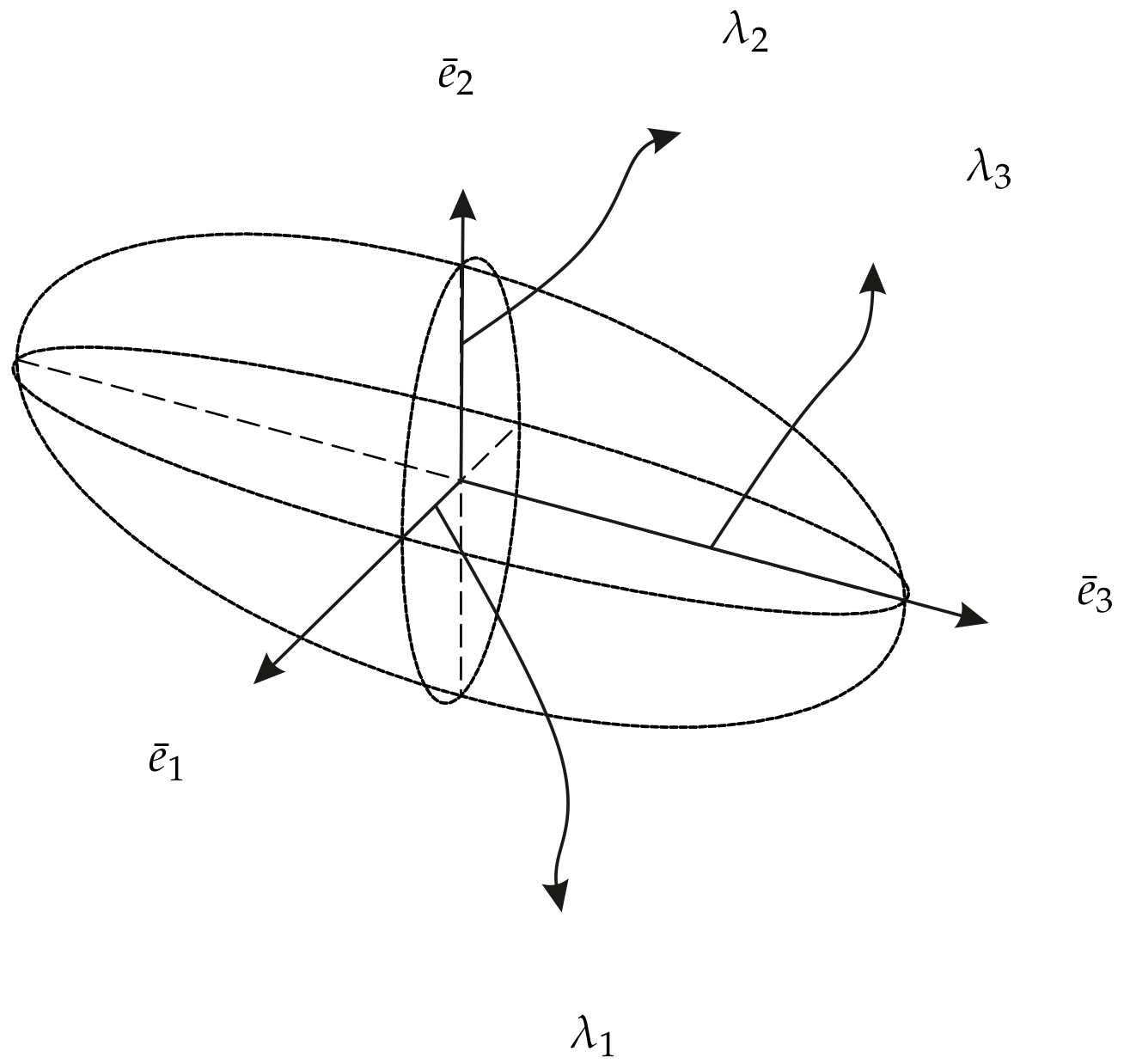
3.2. Proposed Performance Index

As can be seen in Section 3.1, many of the indices mostly rely on the maximum and minimum eigenvalues for performance evaluation. However, this causes a lack in proper stiffness isotropy evaluation for $n\times n$ dimensional stiffness matrix where $n>2$. In this respect, a revision is required for stiffness isotropy index.

While stiffness condition number for a 2 × 2 stiffness matrix regarded as the ratios of radii of a stiffness ellipse, the mathematical meaning behind is the comparison of the areas of a circle and an ellipse. Area of this circle indicates an ideal (desired) performance value which has high isotropy and rigidity. Hence, the square of the maximum eigenvalue is an indication of the area of the circle. Area of the ellipse is the multiplication of all eigenvalues (determinant). The ratio between these areas gives the stiffness condition number. For a 2 × 2 stiffness matrix, this index is formulated as follows:

$$\begin{array}{cc}\hfill {\gamma }_C& =\frac{{\lambda }_2^2}{{\lambda }_1{\lambda }_2}=\frac{{\lambda }_2}{{\lambda }_1}\hfill \end{array}$$

(31)

$$\begin{array}{cc}\hfill {\gamma }_C& \ge 1\hfill \end{array}$$

(32)

The current ${\gamma }_C$ is a 2 DoF evaluation approach and has a lack of performance in the evaluation of 3 or more DoF problems. Therefore, ${\gamma }_C$ cannot distinguish the performances of poses whose eigenvalues ${\lambda }_1={\lambda }_2<{\lambda }_3$, ${\lambda }_1<{\lambda }_2={\lambda }_3$, or ${\lambda }_1<{\lambda }_2<{\lambda }_3$ for 33 matrix. Poses that have closer eigenvalues to maximum one are more isotropic. Hence, ${\gamma }_C$ must be revised for higher DoF evaluation. Higher dimensional isotropy index is the comparison of volumes of an ideal n-dimensional sphere and an n-dimensional ellipsoid. In this regard, the extension of the condition number for $n\times n$ stiffness matrix is a volumetric condition number or volumetric isotropy index that is formulated as follows:

$$\begin{array}{cc}\hfill {\gamma }_I& =\frac{{\Vert \mathit{K}\Vert }_E^n}{det(\mathit{K})}\hfill \end{array}$$

(33)

$$\begin{array}{cc}\hfill {\gamma }_I& \ge 1\hfill \end{array}$$

(34)

where ${\gamma }_I$ volumetric stiffness isotropy index and n is the dimension of the stiffness matrix, nth power of ${\Vert \mathit{K}\Vert }_E$ indicates the volume of the ideal sphere while $det(\mathit{K})$ represented the volume of the ellipsoid. ${\gamma }_I=1$ indicates the isotropic poses in terms of stiffness. Since this index also considers the intermediate eigenvalue contribution, the ambiguity of stiffness performance between the poses that have same ${\gamma }_C$ can be accurately distinguished. Hence, it is expected to have a lower standard deviation of ${\sigma }_I$ compared to ${\sigma }_C$. The standard deviation in such a comparison can be regarded as the preciseness of the performance index.

A volumetric uniformity index ${\gamma }_{IU}$ may also be defined as an extension to ${\gamma }_I$. The uniformity index is defined as follows:

$$\begin{array}{cc}\hfill {\gamma }_{IU}& =\frac{max({\gamma }_I)}{min({\gamma }_I)}\hfill \end{array}$$

(35)

$$\begin{array}{cc}\hfill {\gamma }_{IU}& \ge 1\hfill \end{array}$$

(36)

Since the preciseness of the volumetric stiffness isotropy index is expected to be relatively better, the volumetric uniformity index is expected to be more accurate compared to ${\gamma }_{CU}$.

3.3. Construction of Performance Indices for R-CUBE

Previously mentioned indices are utilized for the stiffness evaluation R-CUBE manipulator, and they are tabulated in

Table 1. Utilized stiffness performance indices.

Index	Matrix	Computed Function	$\overline{\mathit{\mu }}$	$\mathit{\sigma }$	Unit
${\gamma }_V$	${\mathit{K}}_A$	$det({\mathit{K}}_A)$	${\overline{\mu }}_V$	${\sigma }_V$	(N/m)${}^3$
${\Vert .\Vert }_E$	${\mathit{K}}_A$	${\Vert {\mathit{K}}_A\Vert }_E$	${\overline{\mu }}_E$	${\sigma }_E$	(N/m)
${\Vert .\Vert }_1$	${\mathit{K}}_A$	${\Vert {\mathit{K}}_A\Vert }_1$	${\overline{\mu }}_1$	${\sigma }_1$	(N/m)
${\Vert .\Vert }_{\infty }$	${\mathit{K}}_A$	${\Vert {\mathit{K}}_A\Vert }_{\infty }$	${\overline{\mu }}_{\infty }$	${\sigma }_{\infty }$	(N/m)
${\Vert .\Vert }_F$	${\mathit{K}}_A$	${\Vert {\mathit{K}}_A\Vert }_F$	${\overline{\mu }}_F$	${\sigma }_F$	(N/m)
${\gamma }_{ϵ}$	${\mathit{K}}_A$	$\frac{1}{2}{\Vert {\mathit{K}}_A\Vert }_E$	${\overline{\mu }}_{ϵ}$	${\sigma }_{ϵ}$	(Joule)
${\gamma }_I$	${\mathit{K}}_A$	${\Vert {\mathit{K}}_A\Vert }_E^3/det({\mathit{K}}_A)$	${\overline{\mu }}_I$	${\sigma }_I$	-
${\gamma }_C$	${\mathit{K}}_A$	${\Vert {\mathit{K}}_A\Vert }_E/{\Vert {\mathit{K}}_A^{-1}\Vert }_E$	${\overline{\mu }}_C$	${\sigma }_C$	-
${\gamma }_{IU}$	${\mathit{K}}_A$	$max({\gamma }_I)/min({\gamma }_I)$	-	-	-
${\gamma }_{CU}$	${\mathit{K}}_A$	$max({\gamma }_C)/min({\gamma }_C)$	-	-	-

. Since the mobile platform of the manipulator has only translational DoF, translational compliant displacements are our primary interest. Hence, ${\mathit{K}}_A$ sub-matrix is in the focal point of this study.

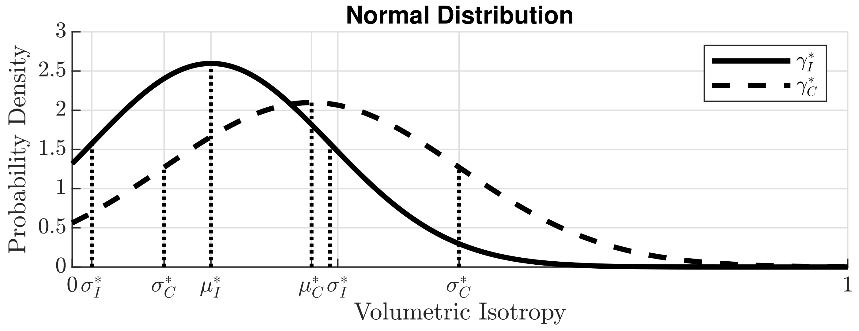
4. Results and Discussion

In this section, only the results on isotropy index calculations are given to present a comparison between the conventional and proposed isotropy index. ${\gamma }_I$, and ${\gamma }_C$ values are computed throughout the workspace, and their results are compared with each other. These computations are carried out by using ${\mathit{K}}_A$ sub-matrix. A normal distribution plot is presented for both indices to illustrate the relative preciseness of the proposed index ${\gamma }_I$. Isotropy indices are computed for each discrete pose of the workspace. Then, the computed indices are illustrated via color mapping.

The maximum and minimum values, average values, standard deviations of isotropy indices are presented in

Table 2. Results of isotropy indices.

	Max	Min	$\overline{\mathit{\mu }}$	$\mathit{\sigma }$
${\gamma }_I$	$5.45$	1	${\overline{\mu }}_I=1.80$	${\sigma }_I=0.68$
${\gamma }_C$	$2.37$	1	${\overline{\mu }}_C=1.42$	${\sigma }_C=0.26$
${\gamma }_{IU}$	$5.45$	$5.45$	-	-
${\gamma }_{CU}$	$2.37$	$2.37$	-	-
${\gamma }_I^{*}$	1	0	${\overline{\mu }}_I^{*}=0.19$	${\sigma }_I^{*}=0.15$
${\gamma }_C^{*}$	1	0	${\overline{\mu }}_C^{*}=0.31$	${\sigma }_C^{*}=0.19$

. Having the minimum value of 1 for ${\gamma }_C$ and ${\gamma }_I$ indices shows that there at least one isotropic pose. By definition of both indices, the isotropy is observed in the same poses. Even though both indices compute the same stiffness matrix, their maximum values differ from each other as expected. The effect of intermediate eigenvalue causes this difference. These maximum values indicate the worst isotropy performance. The number of worst isotropic poses with respect to ${\gamma }_C$ is higher compared to ${\gamma }_I$ because ${\gamma }_C$ does not consider the intermediate eigenvalues. However, the worst isotropic poses concerning ${\gamma }_I$ are also the worst isotropic poses with respect to ${\gamma }_C$, but vice-versa is not necessarily valid for all least isotropic poses.

The values of ${\gamma }_C$ and ${\gamma }_I$ are normalized as ${\gamma }_C^{*}$ and ${\gamma }_I^{*}$ to carry out a fair comparison among them. Accordingly, ${\overline{\mu }}_I^{*}$, ${\overline{\mu }}_C^{*}$, ${\sigma }_I^{*}$, and ${\sigma }_C^{*}$ are obtained in a normalized space. ${\gamma }_C$ and ${\gamma }_I$ are normalized such that the worst performance is denoted by 1 and the highest isotropy is given by 0.

The normal distribution of both indices is compared in a normalized space and shown in Figure 4. Probability density in the vertical axis indicates the number of poses that have the isotropy value denoted in the horizontal axis. Mean values ${\mu }_I^{*}$, and ${\mu }_C^{*}$ indicates the average isotropy of the workspace. ${\gamma }_I^{*}$ results indicate that the workspace is more isotropic with respect to ${\gamma }_C^{*}$ results since ${\mu }_I^{*}<{\mu }_C^{*}$. In addition, the probability distribution of isotropic poses is higher by using ${\gamma }_I$ index. The standard deviation ${\sigma }_I^{*}$ is lower than ${\sigma }_C^{*}$. Hence, ${\gamma }_I^{*}$ is more sensitive to isotropy changes between poses, and this new index can detect slightest changes.

For illustration purposes, 9 planes are selected in the workspace. These planes are parallel to ${\overrightarrow{u}}_1-{\overrightarrow{u}}_2$, ${\overrightarrow{u}}_2-{\overrightarrow{u}}_3$, and ${\overrightarrow{u}}_1-{\overrightarrow{u}}_3$ orthogonal planes. They are divided into 3 groups. In each group, 3 planes are intersect at $[-60,-60,-60]$ mm, $[0,0,0]$ mm, $[60,60,60]$ mm locations of the workspace. Figure 5a and Figure 6a, show the outermost surfaces of the workspace where the planes are placed at $[60,60,60]$ mm. Figure 5b and Figure 6b, show the planes that are coincident at $[0,0,0]$ mm. Figure 5c and Figure 6c, show the most inner surfaces of the workapce at $[-60,-60,-60]$ mm. Due to the symmetric topology of the manipulator, computed performance indices have the same value in several poses. Hence, a symmetric distribution is observed in the results of both indices throughout the workspace.

Due to the definition of both indices, lower values (represented with blue zones) indicate higher isotropy. These areas mainly are observed at the innermost corner, the outermost corner, and at the center of the workspace. However, isotropy distribution differs for ${\gamma }_I^{*}$ and ${\gamma }_C^{*}$ for the rest of the workspace. The transition between low isotropy and high isotropy is more smooth in ${\gamma }_C^{*}$ compared to ${\gamma }_I^{*}$. This smooth transition is a consequence of relatively less precise results obtained with ${\gamma }_C$. Hence, ${\gamma }_C$ cannot precisely distinguish the isotropy levels among poses. However, the transition from low to high isotropy in ${\gamma }_I^{*}$ results illustration is sharper and more distinguishable compared to ${\gamma }_C^{*}$.

Figure 7 and Figure 8 show the iso-curves in ${\overrightarrow{u}}_1-{\overrightarrow{u}}_2$ planes for ${\gamma }_C^{*}$, and ${\gamma }_I^{*}$, respectively. These planes are positioned along ${\overrightarrow{u}}_3$ and they are located at 60 mm,0 mm,$-60$ mm. Figure 8 shows that the covered area by the iso-curves for ${\gamma }_I^{*}=0.1,0.2$ is higher than the area of ${\gamma }_C^{*}=0.1,0.2$ in Figure 7. Hence, ${\gamma }_I$ captures more isotropic poses. Accordingly, iso-curves for ${\gamma }_C^{*}=0.3,0.4,\dots ,0.8$ cover more area than the area covered by the same value of ${\gamma }_I^{*}$. This indicates that the manipulator is less isotropic with respect to ${\gamma }_C$. In addition, notice that the distance between the iso-curves are less for ${\gamma }_I^{*}$ in Figure 8 compared to ${\gamma }_C^{*}$ in Figure 7. Therefore, ${\gamma }_I$ is more sensitive to isotropy changes.

5. Conclusions

In this study, a stiffness model for the R-CUBE manipulator is derived via VJM. A volumetric isotropy index was proposed and compared with the isotropy index that is used in the literature. The proposed index enables a precise evaluation of n-dimensional stiffness problem. The comparison of indices was achieved in a normalized domain. The isotropy distribution is illustrated in 3-dimensional figures using color mapping and by sketching iso-curves. In addition, the normal distribution is given for both indices. It was observed that the proposed isotropy index is more sensitive than the conventional one. It has a lower standard deviation. Hence, it can distinguish isotropic and non-isotropic poses for spatial stiffness matrices, precisely.

While in this paper VJM is chosen to compute the stiffness model, other stiffness model computation can be employed, and the proposed stiffness index and the other indices can be calculated by using these models as well. As a future study, an optimal design will be conducted for R-CUBE mechanism by using the volumetric isotropy index.

References

1. Lian, B.; Sun, T.; Song, Y.; Jin, Y.; Price, M. Stiffness analysis and experiment of a novel 5-DoF parallel kinematic machine considering gravitational effects. Int. J. Mach. Tools Manuf. 2015, 95, 82–96. [Google Scholar] [CrossRef] [Green Version]
2. Dong, C.; Liu, H.; Yue, W.; Huang, T. Stiffness modeling and analysis of a novel 5-DOF hybrid robot. Mech. Mach. Theory 2018, 125, 80–93. [Google Scholar] [CrossRef] [Green Version]
3. Guo, Y.; Dong, H.; Ke, Y. Stiffness-oriented posture optimization in robotic machining applications. Robot. Comput.-Integr. Manuf. 2015, 35, 69–76. [Google Scholar] [CrossRef]
4. Klimchik, A.; Pashkevich, A. Serial vs. quasi-serial manipulators: Comparison analysis of elasto-static behaviors. Mech. Mach. Theory 2017, 107, 46–70. [Google Scholar] [CrossRef]
5. Sun, T.; Lian, B. Stiffness and mass optimization of parallel kinematic machine. Mech. Mach. Theory 2018, 120, 73–88. [Google Scholar] [CrossRef]
6. Courteille, E.; Deblaise, D.; Maurine, P. Design optimization of a delta-like parallel robot through global stiffness performance evaluation. In Proceedings of the 2009 IEEE/RSJ International Conference on Intelligent Robots and Systems, St. Louis, MO, USA, 11–15 October 2009; pp. 5159–5166. [Google Scholar]
7. Wang, H.; Zhang, L.; Chen, G.; Huang, S. Parameter optimization of heavy-load parallel manipulator by introducing stiffness distribution evaluation index. Mech. Mach. Theory 2017, 108, 244–259. [Google Scholar] [CrossRef] [Green Version]
8. Taghvaeipour, A.; Angeles, J.; Lessard, L. On the elastostatic analysis of mechanical systems. Mech. Mach. Theory 2012, 58, 202–216. [Google Scholar] [CrossRef]
9. Arsenault, M. Workspace and stiffness analysis of a three-degree-of-freedom spatial cable-suspended parallel mechanism while considering cable mass. Mech. Mach. Theory 2013, 66, 1–13. [Google Scholar] [CrossRef]
10. Gosselin, C.M. Dexterity indices for planar and spatial robotic manipulators. In Proceedings of the IEEE International Conference on Robotics and Automation, Cincinnati, OH, USA, 13–18 May 1990; pp. 650–655. [Google Scholar]
11. Yan, S.; Ong, S.; Nee, A. Stiffness analysis of parallelogram-type parallel manipulators using a strain energy method. Robot. Comput.-Integr. Manuf. 2016, 37, 13–22. [Google Scholar] [CrossRef]
12. Raoofian, A.; Taghvaeipour, A.; Kamali, A. On the stiffness analysis of robotic manipulators and calculation of stiffness indices. Mech. Mach. Theory 2018, 130, 382–402. [Google Scholar] [CrossRef]
13. Abdolshah, S.; Zanotto, D.; Rosati, G.; Agrawal, S.K. Optimizing stiffness and dexterity of planar adaptive cable-driven parallel robots. J. Mech. Robot. 2017, 9, 031004. [Google Scholar] [CrossRef]
14. Carbone, G.; Ceccarelli, M. Comparison of indices for stiffness performance evaluation. Front. Mech. Eng. China 2010, 5, 270–278. [Google Scholar] [CrossRef]
15. Yeo, S.; Yang, G.; Lim, W. Design and analysis of cable-driven manipulators with variable stiffness. Mech. Mach. Theory 2013, 69, 230–244. [Google Scholar] [CrossRef]
16. Xu, Q.; Li, Y. GA-based architecture optimization of a 3-PUU parallel manipulator for stiffness performance. In Proceedings of the 2006 6th World Congress on Intelligent Control and Automation, Dalian, China, 21–23 June 2006; Volume 2, pp. 9099–9103. [Google Scholar]
17. Liu, X.J.; Jin, Z.L.; Gao, F. Optimum design of 3-DOF spherical parallel manipulators with respect to the conditioning and stiffness indices. Mech. Mach. Theory 2000, 35, 1257–1267. [Google Scholar] [CrossRef]
18. Lee, S.H.; Lee, J.H.; Yi, B.J.; Kim, S.H.; Kwak, Y.K. Optimization and experimental verification for the antagonistic stiffness in redundantly actuated mechanisms: A five-bar example. Mechatronics 2005, 15, 213–238. [Google Scholar] [CrossRef]
19. Pitt, E.B.; Simaan, N.; Barth, E.J. An investigation of stiffness modulation limits in a pneumatically actuated parallel robot with actuation redundancy. In Proceedings of the ASME/BATH 2015 Symposium on Fluid Power and Motion Control, Chicago, IL, USA, 12–14 October 2015; p. V001T01A063. [Google Scholar]
20. Zhou, X.; Jun, S.k.; Krovi, V. Stiffness modulation exploiting configuration redundancy in mobile cable robots. In Proceedings of the 2014 IEEE International Conference on Robotics and Automation (ICRA), Hong Kong, China, 31 May–7 June 2014; pp. 5934–5939. [Google Scholar]
21. Alamdari, A.; Haghighi, R.; Krovi, V. Stiffness modulation in an elastic articulated-cable leg-orthosis emulator: Theory and experiment. IEEE Trans. Robot. 2018, 99, 1–14. [Google Scholar] [CrossRef]
22. Orekhov, A.L.; Simaan, N. Directional Stiffness Modulation of Parallel Robots with Kinematic Redundancy and Variable Stiffness Joints. J. Mech. Robot. 2019, 1–14. [Google Scholar] [CrossRef]
23. Ajoudani, A.; Tsagarakis, N.G.; Bicchi, A. On the role of robot configuration in cartesian stiffness control. In Proceedings of the 2015 IEEE International Conference on Robotics and Automation (ICRA), Seattle, WA, USA, 26–30 May 2015; pp. 1010–1016. [Google Scholar]
24. Ficuciello, F.; Romano, A.; Villani, L.; Siciliano, B. Cartesian impedance control of redundant manipulators for human-robot co-manipulation. In Proceedings of the 2014 IEEE/RSJ International Conference on Intelligent Robots and Systems, Chicago, IL, USA, 14–18 September 2014; pp. 2120–2125. [Google Scholar]
25. Tatlicioglu, E.; Braganza, D.; Burg, T.C.; Dawson, D.M. Adaptive control of redundant robot manipulators with sub-task objectives. Robotica 2009, 27, 873–881. [Google Scholar] [CrossRef] [Green Version]
26. Merlet, J.P. Parallel Robots; Springer Science & Business Media: Berlin/Heidelberg, Germany, 2006; Volume 128. [Google Scholar]
27. Alici, G.; Shirinzadeh, B. Enhanced stiffness modeling, identification and characterization for robot manipulators. IEEE Trans. Robot. 2005, 21, 554–564. [Google Scholar] [CrossRef]
28. Gosselin, C. Stiffness mapping for parallel manipulators. IEEE Trans. Robot. Autom. 1990, 6, 377–382. [Google Scholar] [CrossRef]
29. Kim, H.S.; Tsai, L.W. Design optimization of a Cartesian parallel manipulator. J. Mech. Des. 2003, 125, 43–51. [Google Scholar] [CrossRef]
30. Görgülü, İ.; Kiper, G.; Dede, M.İ.C. A critical review of unpowered performance metrics of impedance-type haptic devices. In Proceedings of the European Conference on Mechanism Science, Aachen, Germany, 4–6 September 2018; pp. 129–136. [Google Scholar]
31. Salisbury, J.K.; Craig, J.J. Articulated hands: Force control and kinematic issues. Int. J. Robot. Res. 1982, 1, 4–17. [Google Scholar] [CrossRef]
32. Paul, R.P.; Stevenson, C.N. Kinematics of robot wrists. Int. J. Robot. Res. 1983, 2, 31–38. [Google Scholar] [CrossRef]
33. Kim, J.O.; Khosla, K. Dexterity measures for design and control of manipulators. In Proceedings of the IEEE/RSJ International Workshop on Intelligent Robots and Systems’ 91 (Proceedings IROS’91), Osaka, Japan, 3–5 November 1991; pp. 758–763. [Google Scholar]
34. Yoshikawa, T. Manipulability of robotic mechanisms. Int. J. Robot. Res. 1985, 4, 3–9. [Google Scholar] [CrossRef]
35. Gosselin, C.; Angeles, J. A global performance index for the kinematic optimization of robotic manipulators. J. Mech. Des. 1991, 113, 220–226. [Google Scholar] [CrossRef]
36. Li, W.; Gao, F.; Zhang, J. R-CUBE, a decoupled parallel manipulator only with revolute joints. Mech. Mach. Theory 2005, 40, 467–473. [Google Scholar] [CrossRef]
37. Dhatt, G.; Lefrançois, E.; Touzot, G. Finite Element Method; John Wiley & Sons: Hoboken, NJ, USA, 2012. [Google Scholar]
38. Klimchik, A.; Chablat, D.; Pashkevich, A. Stiffness modeling for perfect and non-perfect parallel manipulators under internal and external loadings. Mech. Mach. Theory 2014, 79, 1–28. [Google Scholar] [CrossRef] [Green Version]
39. Deblaise, D.; Hernot, X.; Maurine, P. A systematic analytical method for PKM stiffness matrix calculation. In Proceedings of the 2006 IEEE International Conference on Robotics and Automation (ICRA 2006), Orlando, FL, USA, 15–19 May 2006; pp. 4213–4219. [Google Scholar]
40. Ghali, A.; Neville, A.; Brown, T.G. Structural Analysis: A Unified Classical and Matrix Approach; CRC Press: Boca Raton, FL, USA, 2014. [Google Scholar]
41. Pashkevich, A.; Chablat, D.; Wenger, P. Stiffness analysis of overconstrained parallel manipulators. Mech. Mach. Theory 2009, 44, 966–982. [Google Scholar] [CrossRef] [Green Version]
42. Wu, G.; Bai, S.; Kepler, J. Mobile platform center shift in spherical parallel manipulators with flexible limbs. Mech. Mach. Theory 2014, 75, 12–26. [Google Scholar] [CrossRef]
43. Hoevenaars, A.G.; Lambert, P.; Herder, J.L. Jacobian-based stiffness analysis method for parallel manipulators with non-redundant legs. Proc. Inst. Mech. Eng. Part C J. Mech. Eng. Sci. 2016, 230, 341–352. [Google Scholar] [CrossRef]
44. Klimchik, A. Enhanced Stiffness Modeling of Serial and Parallel Manipulators for Robotic-Based Processing of High Performance Materials. Ph.D. Thesis, Ecole des Mines de Nantes, Nantes, France, 2011. [Google Scholar]
45. Pashkevich, A.; Klimchik, A.; Chablat, D. Enhanced stiffness modeling of manipulators with passive joints. Mech. Mach. Theory 2011, 46, 662–679. [Google Scholar] [CrossRef] [Green Version]
46. Carbone, G. Stiffness analysis and experimental validation of robotic systems. Front. Mech. Eng. 2011, 6, 182–196. [Google Scholar]
47. Görgülü, İ.; Dede, M. Computation Time Efficient Stiffness Analysis of the Modified R-CUBE Mechanism. In Proceedings of the International Conference of IFToMM ITALY, Cassino, Italy, 29–30 November 2018; Springer: Berlin/Heidelberg, Germany, 2018; pp. 231–239. [Google Scholar]
48. Stocco, L.; Salcudean, S.; Sassani, F. Matrix normalization for optimal robot design. In Proceedings of the 1998 IEEE International Conference on Robotics and Automation, Leuven, Belgium, 16–20 May 1998; Volume 2, pp. 1346–1351. [Google Scholar]
49. Angeles, J. Fundamentals of Robotic Mechanical Systems; Springer: Berlin/Heidelberg, Germany, 2002; Volume 2. [Google Scholar]
50. Khan, W.A.; Angeles, J. The kinetostatic optimization of robotic manipulators: The inverse and the direct problems. J. Mech. Des. 2006, 128, 168–178. [Google Scholar] [CrossRef]
51. Cardou, P.; Bouchard, S.; Gosselin, C. Kinematic-sensitivity indices for dimensionally nonhomogeneous jacobian matrices. IEEE Trans. Robot. 2010, 26, 166–173. [Google Scholar] [CrossRef]
52. Cao, W.a.; Ding, H.; Zhu, W. Stiffness modeling of overconstrained parallel mechanisms under considering gravity and external payloads. Mech. Mach. Theory 2019, 135, 1–16. [Google Scholar] [CrossRef]
Figure 1. Kinematic sketches of the R-CUBE mechanism: (a) The manipulator, (b) variables of ith serial chain where i is one of the serial chains.
Machines 07 00044 g001
Figure 2. Compliant kinematics of the manipulator where AJ is active joint, PJ is passive joint, VJ is virtual joint, MP is mobile Platform, and B is base.
Machines 07 00044 g002
Figure 3. Illustration of eigenvalues ( λ i for i = 1 , 2 , 3 ) and eigenvectors ( e ¯ i for i = 1 , 2 , 3 ) as an ellipsoid for a 3 × 3 stiffness matrix.
Machines 07 00044 g003
Figure 4. Normal distribution of γ I and γ C .
Machines 07 00044 g004
Figure 5. Isotropy distribution: (a) Outer surfaces, (b) middle surfaces, (c) inner surfaces.
Machines 07 00044 g005
Figure 6. Volumetric isotropy distribution: (a) Outer surfaces, (b) middle surfaces, (c) inner surfaces.
Machines 07 00044 g006
Figure 7. Normalized isotropy iso-curves: (a) 60 mm along u 3 , (b) 0 mm along u 3 , (c) 60 mm along u 3 .
Machines 07 00044 g007
Figure 8. Normalized volumetric isotropy iso-curves: (a) 60 mm along u 3 , (b) 0 mm along u 3 , (c) 60 mm along u 3 .
Machines 07 00044 g008