Optimizing Weight of Housing Elements of Two-stage Reducer by Using the Topology Management Optimization Capabilities Integrated in SOLIDWORKS: A Case Study

Abstract

This paper presents the results of a conducted topology management optimization study based on the finite element analysis on a two-stage spur gear reducer housing body and cover using the SOLIDWORKS Simulation module. The main goal of the study is to optimize the overall weight of the reducer by thinning specific areas of the casted gearbox housing elements according to the calculated minimal strain energy. The topology optimization algorithm that is used in current research gives an optimal structural shape of the housing elements of the reducer with the largest stiffness, considering the given amount of mass that will be removed from the initial design space. The complete sequence of steps for conducting the topology management optimization study is shown, taking into account the constraints arising from the construction features and the method of manufacturing the housing elements of the gear reducer. Conclusions on the use of the topology optimization results are given and potential directions for further development of the approach are also identified.

1. Introduction

Toothed gear reducers are the most commonly used mechanisms for changing the motion parameters and torque in the operation of many different machine actuators, lifting and transporting devices in many manufacturing industries, and in automotive, shipbuilding, aerospace, etc. For obtaining the needed direction of movement and (usually high) transmission ratios, gear reducers may have one or more stages, being equipped with cylindrical gears (with parallel axes), conical gears (with concurrent axes), worm gears (with cross axles), or with a combination thereof. They usually are made with fixed axles but they can also be movable, for example, in planetary or differential gear reducers, which results in a higher transmission ratio with smaller overall dimensions of the reducer. In addition, the toothed wheel gear reducers have a relatively simple construction, high efficiency, and they are easy to install and maintain [1,2,3,4].

Regardless of the type of gear reducer, however, in order to be able to operate reliably and to meet its functional requirements, the relative position of the shafts (respectively the position of the gear wheels and bearings) of the reducer must be precisely fixed in space. An important role in achieving this requirement has two main elements of the gear reducer housing—the lower part (or the body) and the upper part (or the cover). In addition, suitable roller bearings are mounted and fixed by these two gear reducer housing parts in order to balance and transmit the reaction forces from the gears to the foundation to which the gear reducer is mounted. The housing cover usually is fastened to the housing body by bolts and nuts, and the body is mounted on the foundation using anchor bolts. An important role in ensuring the rigidity of the gear reducer has a degree of tightening (i.e., axial loads) of the screw connections.

Despite the diversity of the existing designs of the gear housing, they are mainly produced in two ways: as welded structures made of steel sheets in the case of small-scale production, or by a sand casting process using gray cast iron, in large-scale production. In the case of sand casting of the gear housing elements, a number of requirements arising from good practice in the casting process and subsequent machining operations are recommended to be followed. This includes the requirements as follows [1,2,3,4,5,6,7]:

• The thickness of the wall must be as uniform as possible, in order to avoid any hot tears, shrinkage cavities, or incomplete cavity filling of the sand casting form; additional ribs in the construction are recommended to be used in order to increase the filling ability, strength, and stiffness of the castings;
• Ensuring a certain minimal thickness of the walls of housing casting, depending on the properties of the material used and the casting technology;
• To reduce residual stresses in the castings, smooth transitions from thick to thin sections of the walls should be provided;
• To facilitate removal of the castings from the sand molds, large enough inclines and rounding of the corner of the walls of the gear reducer housing must be provided;
• Machined surfaces must be reduced to the smallest needed number. They are usually limited to machining of the bearing holes, the contact surfaces of the body flanges and the cover, the holes for the fastening bolts, the bearing covers, the threaded plugs, etc.

When the housings of gear reducers are manufactured by the casting process, designers usually follow some general guidance in determining the sidewall thickness, the thickness and width of the bearing flanges, the thickness of the supporting ribs, the diameters of the bolts for attaching the cover to the body or the reducer to the foundation, etc. In the manuals [1,2,3] for constructing transmissions can be found available empirical formulas for calculating the values of these parameters as they are based on pre-calculated diameters of shafts and rolling bearings, the largest distance between axes of the reducer shafts, or the nominal torque at the output shaft. The authors of the gear design guidelines note that the values calculated in that manner are approximate and it is recommended to be followed in the production process. In order to simplify the design process, the dimensions calculated by the empirical formulas are kept the same for all sidewalls, ribs, flanges, and fastening bolts.

Although the requirements for the gear reducer housing are largely satisfied, the described approach does not allow for optimal design solutions, in line with today’s increased production requirements, such as lower weight products, reduced material consumption, less energy consumption per unit of production, environmental protection, etc. In this respect, the present work has the primary objective to demonstrate a different approach for optimal designing of gear reducer housings that optimize the distribution of the material in the body and the cover parts while preserving their stiffness.

2. Topology Management Optimization Approach Description

From about 40 years ago, the topology management optimization approach has achieved rapid development and has been successfully applied to the design of parts in many industrial fields, including the aerospace, automobile, and even biomedical industries. Many different topology optimization methods have been proposed during the years. These include some methods [8,9] gaining wider popularity like the level set methods [10,11], the density approach [12], evolutionary approaches (evolutionary structural optimization/bi-directional evolutionary structural optimization, ESO/BESO) [13], and several others. 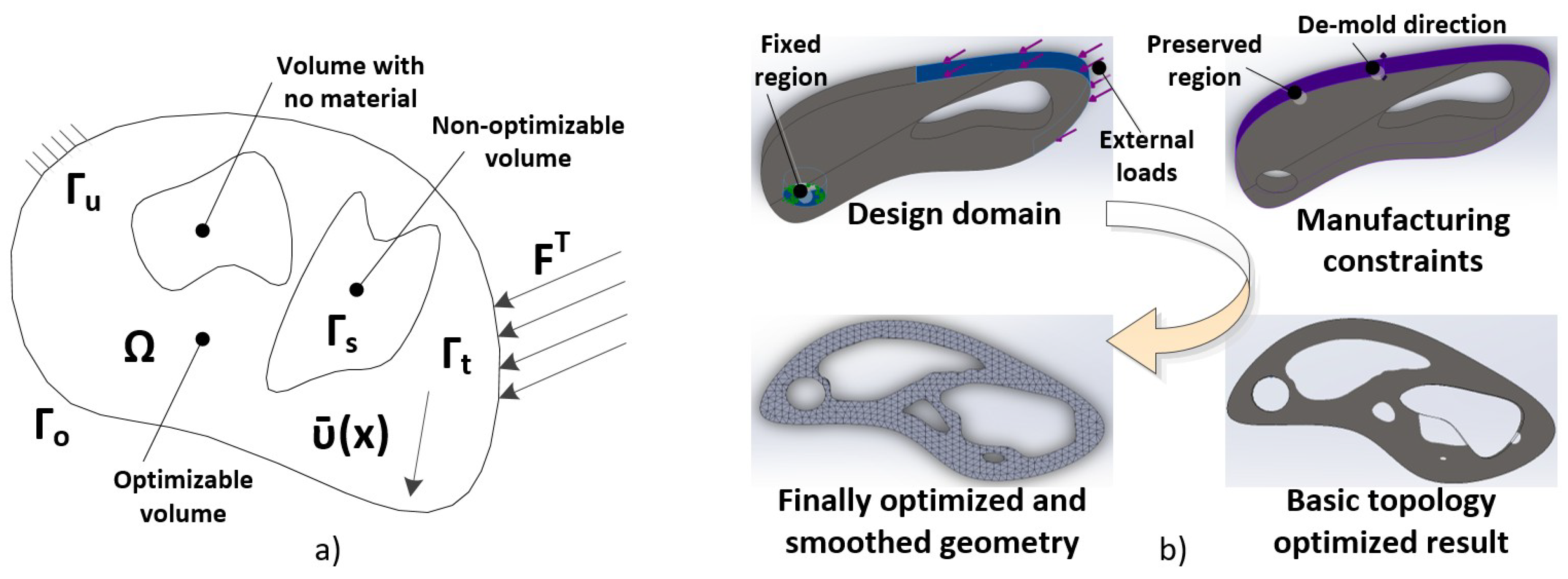There are also a number of variations and modifications of these basic methods aimed at solving specific optimization problems [8]. In general, topology optimization is a mathematical method that optimizes material layout within a given design space Ω, as shown in Figure 1a. Usually it uses given design space Ω, loads condition L, boundary conditions Γ consisting of Γ_o, Γ_s, Γ_t, and Γ_u parts, where Γ = Γ_u ∪ Γ_o ∪ Γ_t ∪ Γ_s and one or more manufacturing constraints. The surface tractions “t” are applied at region Γ_t; regions Γ_u represent the support conditions; regions Γs denote the non-optimizable areas; and Γo are the geometric boundaries of the design space Ω.

For finding the optimum layout of a structural system composed by linearly elastic isotropic material, the material distribution methods can be used [14]. The main question here is how to distribute material volume into domain Ω in order to minimize a specific criterion. The usually most used criterion is the compliance C. Density values x (distributed over the domain Ω) are used to control the distribution of the material volume in the domain. It is controlled by design parameters that are represented by the densities x assigned to the finite element (FE) discretization of domain Ω. The densities x take values in the range (0−1), where zero means no material in the specific point (s).

A topology management optimization problem can be written in the general form as [14]

$$\begin{array}{ll}\mathrm{minimize}\mathrm{x}& C\left(x\right)=F^T·\overline{u}\left(x\right)\\ \mathrm{subject}\mathrm{to}:& \frac{V\left(x\right)}{V_0}=f\\ & F=K\left(x\right)·\overline{u}\left(x\right)\\ & 0<x_{min}\le x\le 1.\end{array}$$

(1)

where:

• C(x) represents the compliance of the structure;
• F^T is an applied vector of forces;
• $\overline{u}\left(\mathrm{x}\right)$ denotes the corresponding global displacement vector.

The second expression of Equation (1) refers to a volume constraint, where f is the volume fractions of domain Ω that the optimized layout should occupy. The global stiffness matrix K(x) of the structural system takes place in the third expression of Equation (1) and corresponds to the equilibrium equation, and the last inequality represents the definition set of the density values.

The topology optimization approach usually involves four major stages, as shown in Figure 1b. The first phase includes the definition of the original (i.e., not optimized) 2D or 3D geometry of the object. The following model parameters are set here: the design material characteristics, the fixed surfaces of the model, the surfaces to which the external loads are applied, the type and magnitude of the external loads, etc. The second phase involves setting manufacturing constraints, such as preserved regions that will not be modified during a topology optimization, de-mold direction, load symmetry about a specified plane, minimum wall thickness that prohibits the creation of very thin or very thick regions that may be difficult to manufacture, etc. The third stage involves obtaining the basic topology optimized result after the FE analysis is performed. At this step, it is possible to adjust the volume ratio of the remaining and removed material precisely, as well as to use surface smoothing algorithms in order to remove or modify elements that create jagged edges and/or sharp angles. At the last stage of the topology optimization process, Computer Aided Design (CAD) software tools are used to transform the “organic looking” areas from the optimized model into simpler ones in order to facilitate the manufacturing process.

Topology optimization modules have been developed and integrated into many contemporary CAD-CAE (Computer Aided Engineering) software products for 2D and 3D designing, such as SIMULIA Abaqus and Tosca Structure (Dassault Systèmes, Vélizy-Villacoublay, France), SOLIDWORKS (SolidWorks Corporation, Waltham, MA, USA), ANSYS (ANSYS, Inc., Canonsburg, PA, USA), Fusion 360, Inventor and Nastran (Autodesk, Inc., San Rafael, CA, USA), COMSOL Multiphysics^® (COMSOL, Inc., Stockholm, Sweden), etc. Topology optimization capabilities are also integrated into some freeware open source 3D software products such as Blender, Top3d, etc. A more detailed list of software products that support topology optimization capabilities can be found in Reference [15].

3. Case Study of Weight Optimizing of Spur Gear Reducer Housing

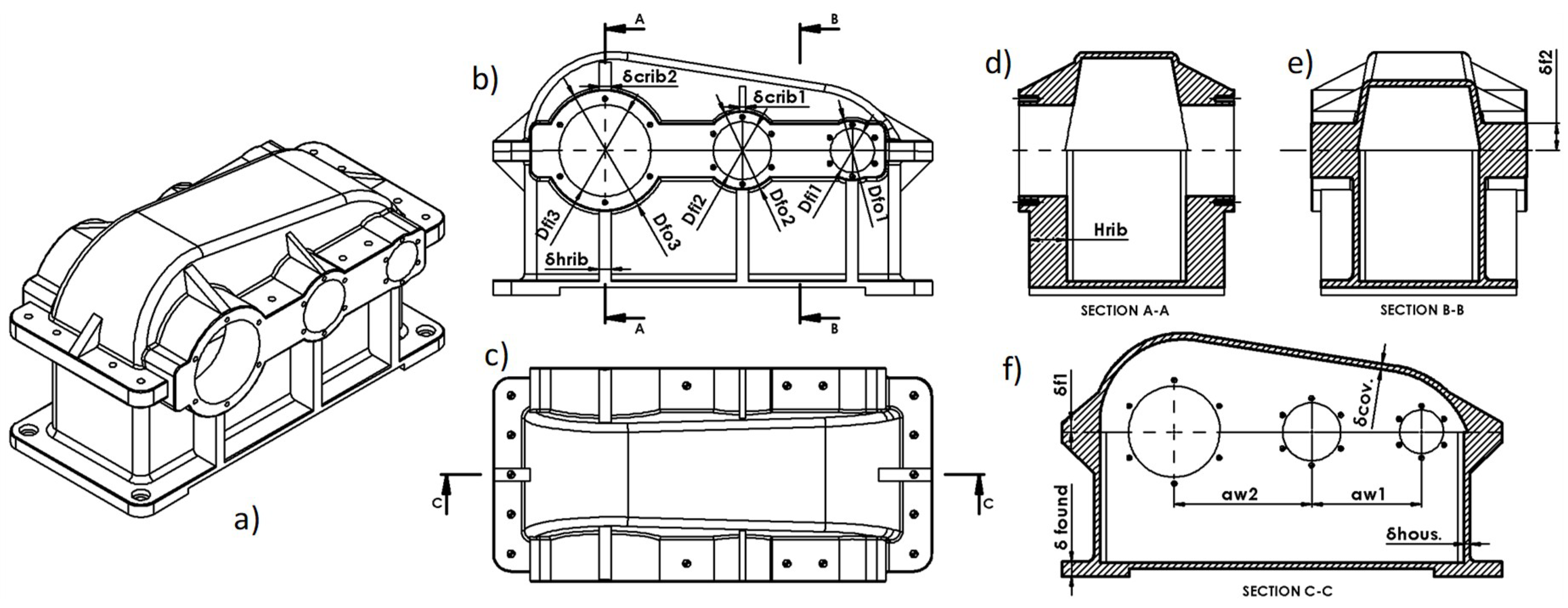
According to the primary objective of the present work, in this section the main steps of the process for topology management optimization will be described using a specific case study of a two-stage gear reducer housing and cover, whose constructive features are presented in Figure 2a–e.

3.1. Initial Constructive Features of the Housing and Cover of the Reducer

In the Figure 2 are presented two views, as shown in Figure 2b,c, and three section views, as shown in Figure 2d–f, on which the dimensions of the constructive elements of a spur gear reducer housing and cover (assembled to each other) are shown.

The dimension labels and their calculated values are shown in

Table 1. Calculated dimensions’ values of the characteristic elements of the housing body and cover.

Dimension Labels	Empirically Calculated Values (mm)	Description
δcov.	9.0	Thickness of the side walls of reducer cover
δhous.	10.0	Thickness of the side walls of reducer housing
δf1	17.0	Thickness of the side part of reducer cover flange (side part of reducer housing flange has the same value)
δf2	45.0	Thickness of the front part of reducer cover flange (front part of reducer housing flange has the same value)
δfound.	24.0	Thickness of the foundation of the reducer
δhrib	15.0	Thickness of the housing ribs located below bearing seats
δcrib1	10.0	Thickness of the cover rib located above bearing seat
δcrib2	10.0	Thickness of the cover rib located above bearing seat
Hrib	164.0	Height of the housing ribs located below bearing seats
aw1	180.0	Distance between axes of the shafts on first stage
aw2	225.0	Distance between axes of the shafts on second stage
δb1= Dfo1 − Dfi1	14.0	Thickness of the bearing seats around the input shaft
δb2= Dfo2 − Dfi2	17.5	Thickness of the bearing seats around the middle shaft
δb3= Dfo3 − Dfi3	25.0	Thickness of the bearing seats around the output shaft

. The values were calculated using the empirical equations or table data with recommended values, purposed in the References [2,3].

3.2. Preparatory Steps for Topology Optimization Process

In order to perform needed finite element analysis and carry out topology management optimization of the objects using the simulation module of SOLIDWORKS [16], the following particular steps must be completed.

3.2.1. Digitization of the Model

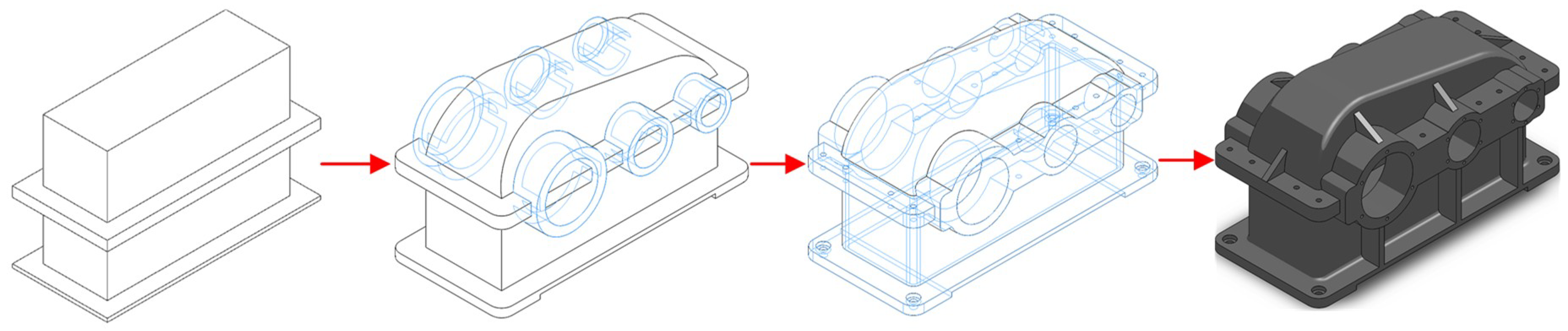
The digitization process of the model was carried out using the 3D modeling capabilities and powerful design automation tools integrated in SOLIDWORKS. Although, in reality the housing and the cover of the gear reducer are separate parts, here they were modelled as a single (monolithic) body, as shown in Figure 3. This is an important condition, because the topology optimization module of SOLIDWORKS does not allow simultaneous optimizing of several parts or assemblies. In order to speed up the process of topology optimization, the construction of the 3D model was simplified by removing some auxiliary elements such as oil inlets, vents, oil level indicators, service hatch, etc.

In the case that the housing elements are pre-modelled as separate parts, in order to be able to perform the topology optimization in SOLIDWORKS, they must be combined into a single body.

3.2.2. Material Selection

Gray cast iron G150 (according ISO 185 [17]) was selected as a material of the 3D model, because the housing body and cover parts will be produced by the sand casting method. It is a widely used material in heavier gearboxes, which have sufficient rigidity and good vibration damping properties. The grade G150 cast iron material used in model had the following mechanical characteristics: elastic modulus = 66,178.1 (N/mm²); Poisson’s ratio = 0.27; shear modulus = 50,000 (N/mm²); mass density = 7200 (kg/m³); tensile strength = 151.66 (N/mm²); Compressive Strength = 572.17 (N/mm²).

The Material Dialog Box of the SOLIDWORKS was used to assign the material to the 3D model.

3.2.3. Defining the External Loads and Fixtures

The loads of the housing elements depend on the constructive configuration of the gear reducer and its specific input parameters. They usually involve: transmission ratio i; inclination angle of the teeth β, (^°) in case of helical gears; the transmitted power P, (kW); the input speed n₁, (rev/min), and the largest required distance between axes a_w^max, (mm), and they can be separated into two main groups:

• The radial loadsFR_i,X and FR_i,Y, i = 1, 2, 3. They were transmitted by the rolling bearings to the bearing seats and cause contact stresses. They arose from the radial and tangential forces acting on the toothing of the spur gear wheels. When the reducer has helical gears, axial load occurs. The direction of this load was parallel to the axes of the shafts and must also be taken into account in the calculations;
• The axial loads in “bolt-nuts” connections for fastening the gear reducer to the foundation and for the bolts fastening the cover flange to the flange of the housing body.

The values of these loads can be calculated for each particular gearbox configuration using well-known techniques and formulas from Statics and Strength of Materials [1,2,18]. The spur gear reducer considered in this work has the input parameters that are shown in

Table 2. Main input parameters of the reducer.

Parameter	Value
Transmission ratio, i	22.78
Inclination angle of the teeth, β	0 (°), spur gears
Transmitted power, P	6.3 (kW)
Input speed, n1	1450 (rev/min)
Max distance between axes, awmax	see Table 1

. The spur gears from the stages were designed according to them using specialized software MITCalc [19], and the values of the radial load FR_i,X and FR_i,Y, i = 1, 2, 3 were calculated for the six roller bearings of the reducer, as shown in

Table 3. Calculated values of the radial loads in bearings.

Shaft №	Loads in the Bearings on the Left Side			Direct. of FRL	Loads in the Bearings on the Right Side			Direct. of FRR
	FRX, (N)	FRY, (N)	FRL, (N)	αL, (°)	FRX, (N)	FRY, (N)	FRR, (N)	αR, (°)
1	2364.38	1930.76	3052.56	50°, 46’	−21.07	1684.88	1685.02	359°, 11’
2	−28.92	−100.71	104.77	106°,01’	1257.11	3460.85	3682.09	19°, 57’
3	1551.90	4263.81	4537.45	20°,00’	789.81	2169.97	2309.24	20°,00’

.

The resultant magnitudes of bearing loads FR_i (i = 1, 2, 3), as shown in Table 3, applied in the bearing seats from left (L) and the right (R) side of the reducer were calculated as a vector sum using the equation

$$F{R}_i^{\left(\mathrm{L},\mathrm{R}\right)}=\sqrt{F{R}_{i,X}^{\left(\mathrm{L},\mathrm{R}\right)}{}^2+F{R}_{i,Y}^{\left(\mathrm{L},\mathrm{R}\right)}{}^2} \left(i=1,2,3\right),\left(\mathrm{N}\right).$$

(2)

The angles α_i^(L,R) of direction of resultant loads vector FR_i (i = 1, 2, 3) are calulated by use FR_X and FR_Y values of the reactions components in horizontal and vertical direction and sine, cosines, or tangent trigonometric functions. The calculated values for α_i^(L,R) are shown in Table 3 also.

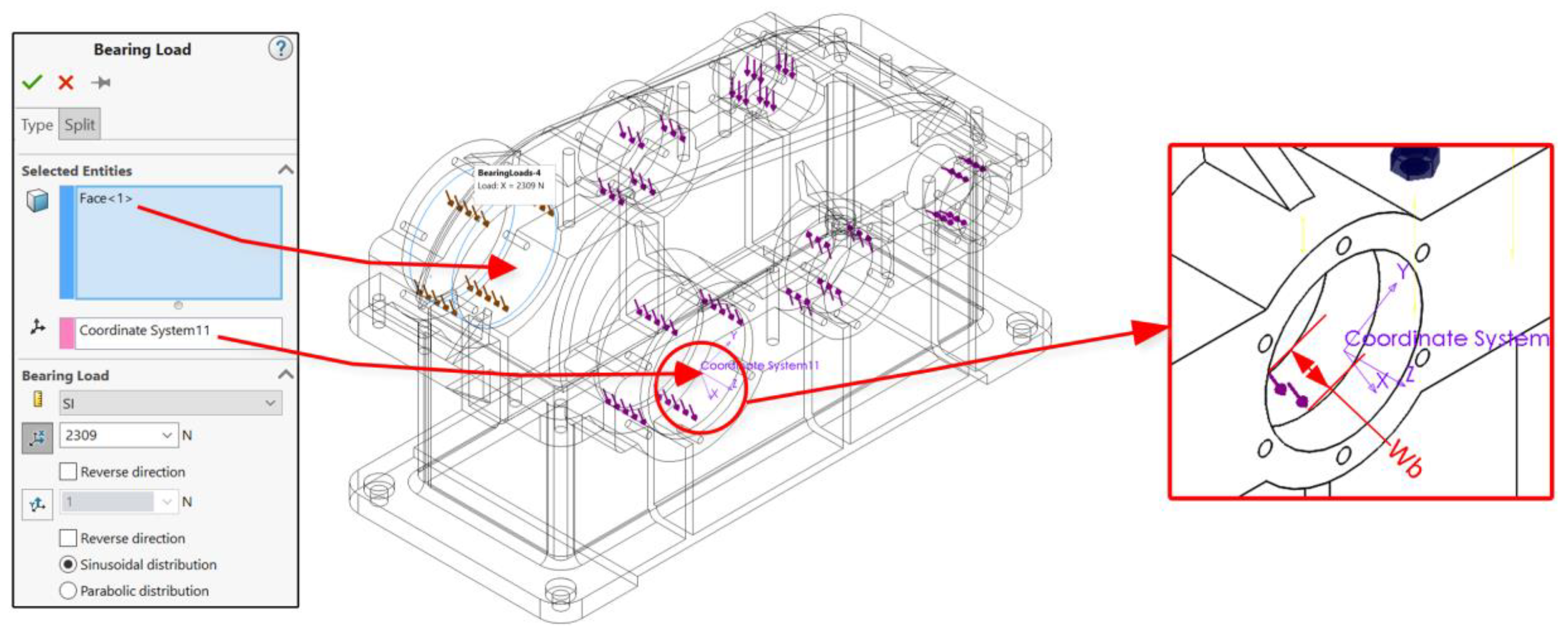
The calculated values of resultant loads FR_i^(L,R) by Equation (2) in Table 3 were set as a bearing load component [20] with sinusoidal distribution for every bearing seat in the 3D model in the section “External loads” of the SOLIDWORKS Simulation, as shown in Figure 4. The Bearing Load was used because this component distributes the applied bearing loads radially and non-uniformly along the cross-section of a cylindrical faces of the bearing seats. Thus, the bearing load are applied to the half of the selected faces only. In order to correctly set the loads, the cylindrical faces on which it is applied have a lesser width Wb, as shown in Figure 4, than the total width W of the bearing seats. Usually the dimension Wb is equal to the width of the chosen roller bearing. The directions of the applied bearing loads were defined using different Coordinate Systems in SOLIDWORKS. The Z-axis was always coincident with the rotating axis of the bearing, and the X-axis must be rotated at previously calculated angles α_i^(L,R).

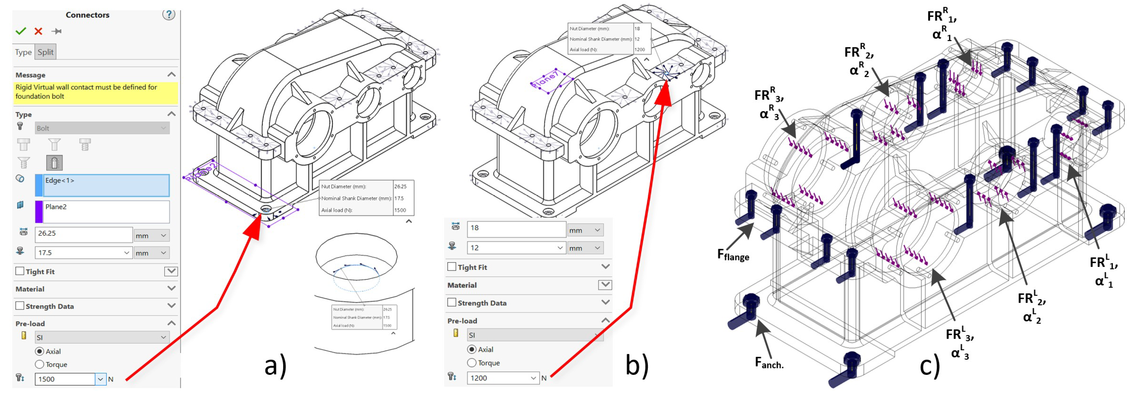
The axial loads in preloaded anchor bolt-nut connections and those in the flanges of the cover and base body were also calculated using MITCalc software. The obtained values were respectively 1500, (N) for anchor bolts, and 1200, (N) for flange connections. These two values were set in the SOLIDWORKS 3D model as bolt-connectors, as it is shown in Figure 5a,b.

The 3D model of the reducer housing with all bearing loads and fastening axial forces applied, produced by the fixtures, is shown in Figure 5c.

3.2.4. Defining Goals and Constraints of the Model

In this section of the topology optimization study, the optimization goals and constraints must be chosen. The topology study will try to find the stiffest structure possible given a certain amount of material removal. Defining the goal and constraints will impact the material removal. The optimization algorithm gives the shape of the most rigid components of the 3D model, defined by the amount of mass that will be removed from the original maximum design space Ω. When the “Best Stiffness to Weight ratio” option is selected, the algorithm will try to minimize the global compliance of the 3D model which is a measure of the overall flexibility (contrary to stiffness). Compliance is defined by the sum of strain energies of all elements. Constraints limit the Ω-space solutions by imposing the percentage of the mass that can be removed to be under a certain value, or by setting limits for the maximum displacement observed in the 3D model. In SOLIDWORKS Simulation (version 2018), up to two constraints for one optimization goal can be defined at the same time. For the current study, the option “Best Stiffness to Weight ratio” and 30% reduction of the mass, were chosen (i.e., applied settings by default). In this way, from the initial mass of 106.93 (kg) of the considered gear reducer housing, after the topology optimization, theoretically its mass will be reduced to 74.86 (kg) (or by 30%).

3.2.5. Defining the Manufacturing Controls

The topology optimization process creates a layout of the material that corresponds to the optimization goal at the specified geometric constraints. However, the 3D model may be impossible to manufacture using usual manufacturing processes, such as casting or forging. The formation of undercuts and hollow parts can be prevented by applying proper manufacturing controls in the optimization model. Manufacturing restrictions ensure that the optimized 3D model can be extracted from a mold for example, or can be stamped properly. SOLIDWORKS Simulation allows four types of manufacturing controls. They are as follows:

• Thickness Control. Sets a limitation to the topology optimization of the model that prevents the production of too thin walls or very thick regions that would be difficult to manufacture.
• Preserved Region(s). This property adds preserved region(s) to the 3D model that will not be modified during topology optimization, and thus leaving unchanged the geometry of those surfaces that are important to its proper operation.
• Symmetry Control. Symmetry control forces the optimized 3D model to be symmetric to a specified plane or planes. A half, quarter, or one-eighth planar symmetry can be chosen depending on the design configuration.
• De-mold Control. This property can be used to ensure that the optimized 3D model can be extracted from a mold.

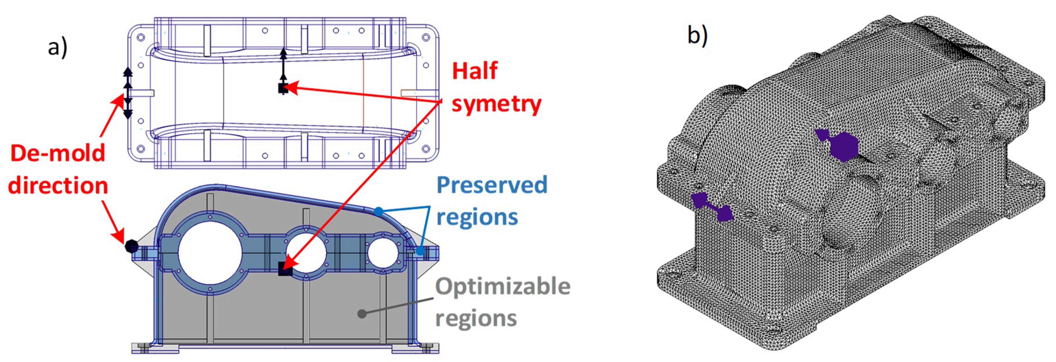
Half-symmetry and de-mold manufacturing controls were used in the current study in addition to several preserved regions, as shown in Figure 6a. Preserved regions in the model include the fundament area of the reducer and flanges both of the body and the cover. As can be seen from Figure 6a, some of the fillets located at the corners and along the edges of the body and the cover are included in the list of the preserved regions. The preservation of these elements of the design aims to facilitate the closure process of the housing elements after topology optimization. The depth of all the preserved regions that will remain unchanged during optimization was set to 8 mm, according to the recommended minimal thickness of the side walls for gray cast iron.

The 3D model is divided into 308,263 finite elements, as shown in Figure 6b, with standard solid mesh which has 498,985 nodes. The minimal element size is 7.25 (mm) with a tolerance of 0.363 (mm) and its size is smaller than the thickness of preserved regions (8 mm).

3.3. Results Obtained after Implementation of the Topology Management Optimization

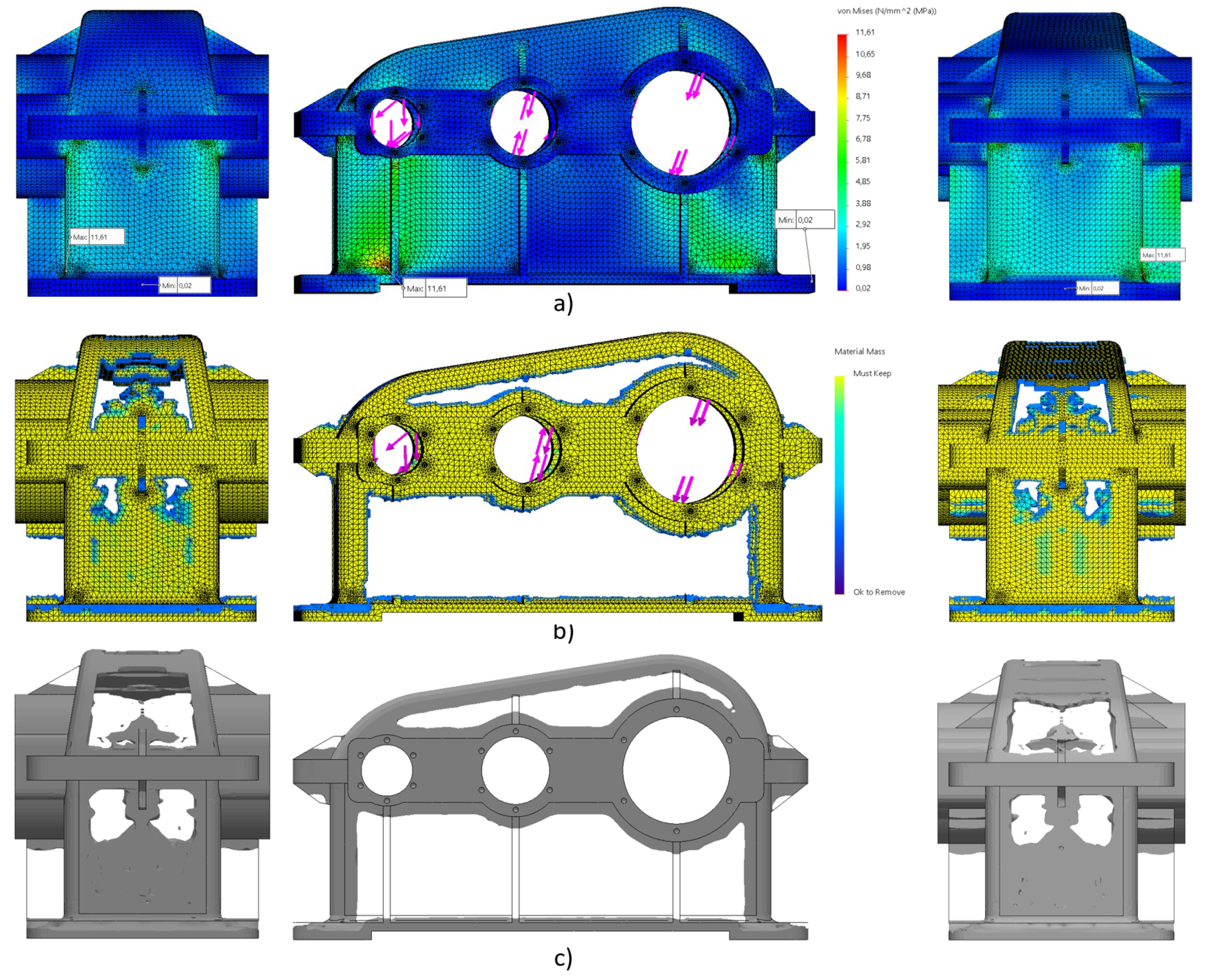
The topology optimization study was carried out using the SOLIDWORKS Simulation module with the particular load scenario, boundary conditions, and manufacturing controls as described in Section 3.2. The resultant stress (von Mises) plots that show the distribution of the stresses in the material of the reducer housing elements are shown in Figure 7a.

Three views of the resultant topology optimized 3D model are shown in Figure 7b. The topology optimization algorithm couple material’s Young’s modulus of each mesh element with a relative mass density factor ranging from 0.0001 for a void element without any load-carrying capacity to 1.0 for a solid element with load-carrying capacity. Here, the “soft” elements selected as “Ok to Remove” (with relative mass density less than 0.3) are deep purple. They do not contribute significantly to the stiffness of the reducer housing elements and were removed from the design. The elements selected by the algorithm as “Must Keep” (with high relative mass densities larger than 0.7) are yellow. After deleting the “soft” elements of the design, the mass was reduced to 73% in comparison to the initial one.

Because the optimized 3D model, shown in Figure 7b, has a very “organic” shape with many jagged edges and sharp angles after the topology optimization, it was not very suitable for further processing and closing the side walls of the reducer housing. For this reason, additional smoothing of the optimized model was carried out with maximum possible iteration cycles to obtain a smoother surface mesh of the optimized model.

The final mass plot of the reducer housing elements after applying additional smoothing of the surfaces is shown in the Figure 7c. After the topology optimization was carried out, the initial mass 106.93 (kg) was reduced to 76.30 (kg) or 71% of the original mass.

4. Post-Processing of the Topology Optimized Gear Reducer Housing and Cover

As it can be seen from Figure 7c, all elements considered as “soft” were removed from the design and the reducer housing elements acquires a near to “building carcass” structure. They cannot be left in this way (as a carcass structure) because in this shape they will not be able to fully meet their functional purpose; besides balancing power loads, also being able to keep the lubricant in the operating area of the gears, and to isolate them from the impact of the environment (such as moisture, dustiness, etc.). Therefore, all voids and openings obtained in the gearbox housing after optimization should be suitably closed. Closure of the gaps in the 3D model can be done by adding material with a minimum wall thickness defined only by the casting manufacturing requirements, and in particular from the fluidity index of the used cast iron grade.

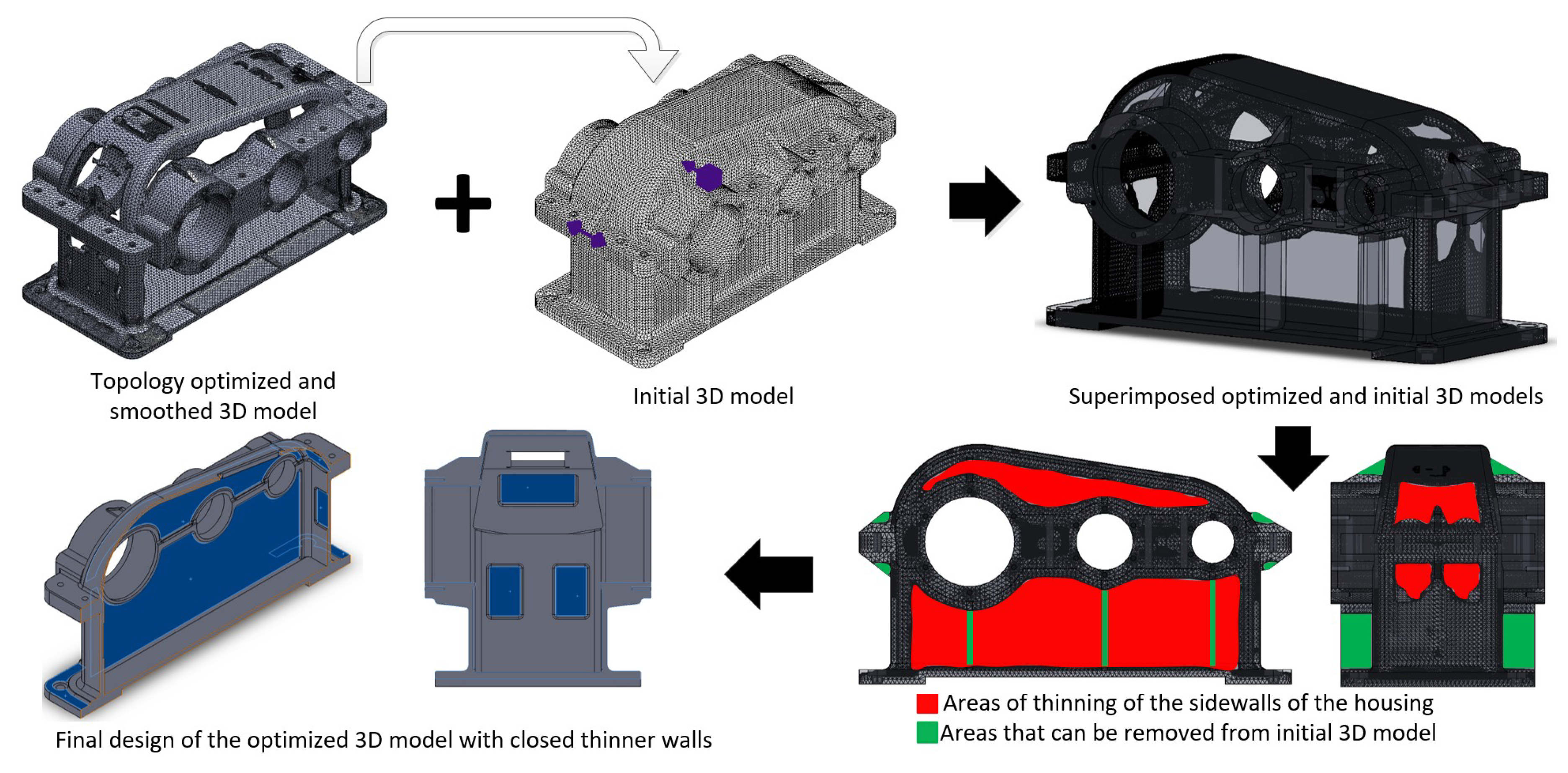
The optimized 3D model can be exported as graphic body, solid body, or surface body. The options “Surface body” and “Solid body” are useful when the model will be printed on a 3D printer without further editing of the design. The option “Graphic body” exports optimized design in the boundary geometry representation format, which is more suitable for further editing and modifying. SOLIDWORKS allows exported graphic body to be inserted in the initial 3D model of the gear reducer housing, as can be seen in Figure 8. The first step after superimposing two 3D models is to estimate the differences between them. The easiest way to do this is to change the transparency of the initial model to semitransparent and keep the optimized model as opaque.

As can be seen from Figure 8, some areas from the sidewalls of the reducer housing elements (coloured in red) are suitable for thinning (because the gear housing can not remain as open structure), while other areas like the material around the lifting holes and the ribs above and below the bearing’s seats (coloured in green) can be partially removed. When modifying the 3D model it is necessary to comply with the requirements for designing parts which are manufactured by sand casting, i.e., minimum sidewall thickness, drafts, and to have rounded transitions between the thin and thick sections of the construction [21,22,23].

Using integrated SOLIDWORKS CAD-tools, all optimized areas were adjusted or removed according to the above mentioned conditions and the final result is shown in Figure 8. Тhe final 3D model can be sliced into two different parts—the housing body and cover, and some additional features, such as holes for oil inlets, vents, oil level indicators, service hatch, etc. can be added to the design. The position of the hole of the upper service hatch is selected in accordance with the topology optimized results of the top side of the housing cover. The mass properties of the initial, the topology optimized, and the final optimized 3D models are shown in

Table 4. Mass properties of the initial, the topology optimized, and the final optimized 3D models.

Mass Properties	Initial 3D Model	Topology Optimized 3D Model	Finally Optimized Model
Mass, (kg)	106.94	76.30	99.10
Volume, (mm3)	14,852,768.38	10,238,437.15	13,902,279.95

.

As can be seen from Table 4, the mass of the topology optimized 3D model was decreased by 28.65%, which is close to the set target value (30%) in the goal parameter of the topology optimization study. The mass of the finally optimized model after adjusting geometry was decreased by 7.33% from those of the initial 3D model.

5. Verification by Static Load and Natural Resonant Frequencies Studies of the Initial and Optimized 3D Models

For verification of the behavior of the optimized 3D design, static load FE-analysis to check the stress levels and displacement, and simulations of the resonant frequencies before and after the optimization of the reducer housing elements, were carried out. In these simulations was used the same load pattern as in the topology optimization study.

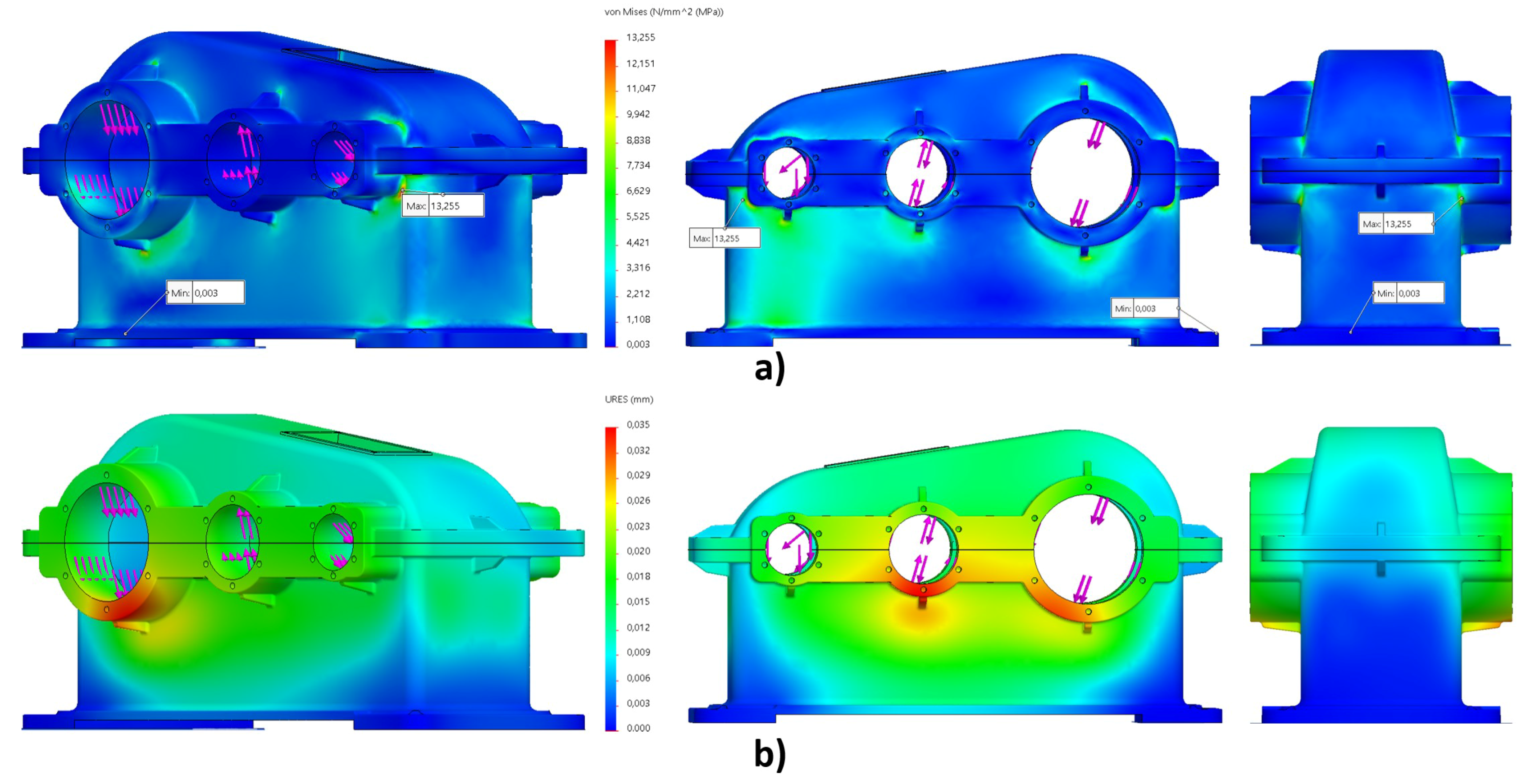
The resultant stresses (von Mises) from the static load simulation is shown in Figure 9a and the displacement diagrams are shown in Figure 9b. As can be seen, the obtained maximum equivalent stress values 13.26 (MPa) were much lower than the modulus of elasticity 6.62 × 10⁴ (MPa) of gray cast iron. Corresponding to the obtained stress values, the maximum displacement value was 0.035 (mm). The minimal obtained factor of safety (FOS) value was 11.44. These static study results show that the final optimized housing 3D model of the reducer will withstand the loads from the gears without the risk of plastic deformation or rupture.

Thinning of the specific areas of the reducer housing and the removal of material from its initial construction will affect the natural resonant frequencies of the finally optimized design. As the gear housing is subjected to forced oscillations, resulting from the transmission of the load on the gears, it is necessary to check for the possibility of falling into resonance after the optimization. For this purpose, two similar natural frequencies studies were carried out, firstly for the initial design of the reducer housing model, and secondly for the finally optimized model. Here, the same load and fixture patterns as in the topology optimization and in the static studies were used again. The obtained results from the studies for the first four modes are shown in

Table 5. Obtained results for the first four modes and natural frequencies.

Mode №	Initial 3D Model		Final Optimized 3D Model		Forced Oscilation
	Frequency (Hz)	Frequency (rev/min)	Frequency (Hz)	Frequency (rev/min)	Frequency (Hz)	Frequency (rev/min)
1	235.48	14,128.8	263.2	15,792.0	24.17	1450
2	316.86	19,011.6	480.28	28,816.8
3	410.66	24,639.6	539.97	32,398.2
4	480.56	28,833.6	552.79	33,167.4
5	509.60	30,576.0	652.62	39,157.2

.

Comparison of the obtained results in Table 5 show that the natural frequencies for the first five modes of the final optimized 3D model are greater than those for the initial 3D model. The increase in natural frequency values is explained by the decrease in mass of the final optimized model while the stiffness of the gearbox housing elements remains almost unchanged due to the nature of the used topology management optimization approach. As can be seen from Table 5, the natural frequencies of the final optimized 3D model was far away in comparison to the frequencies of the forced oscillations. The resonant frequency 263.20 (Hz) or 15.792 (rev/min) for first mode was 10.89 times greater than the highest rotational speed 1450 (rev/min) of the input shaft (or 24.17 (Hz)) of the gear reducer. Therefore, it can be concluded that thinning the sidewalls of the gear reducer housing based on carried out topology management optimization will not lead to falling into resonance condition during its regular operation.

6. Conclusions

Because the topology optimization module of SOLIDWORKS does not allow assemblies to be subjected to the topology optimization algorithm, but only the single part (i.e., the single 3D body), the 3D models of the parts of the housing body and cover were combined into a single 3D body, and the result was saved as a part file. Thus, the limitations of the simulation module were overcome in the presented case study. Additionally, as demonstrated by the exemplary topology optimization of the gear reducer housing, the embedded algorithm in SOLIDWORKS Simulation can be successfully applied even for relatively complex 3D models of device and machine housings.

Another point that must be considered were the results obtained from the static stress analysis and nodal displacements of the topology optimized and smoothed 3D model, as shown in Figure 7c. In the simulation results section of SOLIDWORKS, there is a notification which alerts that the obtained values are based on the entire optimized model which may contain porous elements that are less rigid than fully dense elements. For this reason, these values should be thought of as a rough estimate on how the topology optimized model might behave [16]. For example, in the present topology optimization study, the obtained values for the static stress reach 4943.94 (MPa) and the obtained maximal nodal displacement is 15.45 (mm), which obviously can not be achieved by real physical construction. Therefore, it is not advisable to take these results as valid, and static analysis should be conducted on the final closed 3D design, as shown in Figure 9, as it was described in Section 5. To avoid obtaining resonance, the natural frequencies must be determined before and after the topology based optimization of the model, and they should be compared to the frequency of forced oscillations arising from the drive of the gearbox. For stable and reliable operation of the device, there must be no approximation between them.

By applying the finite element method to analyse an exemplary gear reducer housing element and carried out topology optimization, a reduction in the total weight of these parts within about 7.33% has been achieved. At first glance, this may not sound like a very large reduction in the weight of the gear reducer, relative to a single piece of a product, but with a larger production series, the effect of saving the material will be felt. The proposed approach can also be applied to the optimization of the housing elements of heavy gear reducers and gearboxes, which are usually designed with increased factors of safety; for example, for use in large ships and marine equipment, as well as in lifting, construction, and/or metalworking machinery.

In conclusion, it should be noted that the results obtained in the present work are strictly related to the used model and construction of gearbox and its input parameters, as shown in Table 2. In other gear designs and operational parameters, topology management optimization results may differ materially from those shown in this work. Therefore, each construction should be considered individually, in accordance with the constructional features and requirements of the final product.

It should also be noted that the presented topology management optimization was based only on the load of the housing elements of the gear reducer. It did not include some additional factors, such as gearbox heating, noise emissions, etc., which may also affect its design parameters. Opportunities for further development of the present work can be the creation of approaches and algorithms for implementing the topology management optimization approach of similar three-dimensional housing bodies of other types of devices and machines, taking into account the influence of additional factors in their operation, besides only the work load from the transmitted forces, torques, and/or reactions in the bearings.