Article

Regression Model for the Prediction of Total Motor Power Used by an Industrial Robot Manipulator during Operation

Faculty of Engineering, University of Rijeka, Vukovarska 58, 51000 Rijeka, Croatia
*
Author to whom correspondence should be addressed.
These authors contributed equally to this work.
Machines 2024, 12(4), 225; https://doi.org/10.3390/machines12040225
Submission received: 26 February 2024 / Revised: 26 March 2024 / Accepted: 26 March 2024 / Published: 28 March 2024
(This article belongs to the Special Issue Design and Control of Electrical Machines II)

Abstract

:
Motor power models are a key tool in robotics for modeling and simulations related to control and optimization. The authors collect the dataset of motor power using the ABB IRB 120 industrial robot. This paper applies a multilayer perceptron (MLP) model to the collected dataset. Before the training of MLP models, each of the variables in the dataset is evaluated using the random forest (RF) model, observing two metrics-mean decrease in impurity (MDI) and feature permutation score difference (FP). Pearson’s correlation coefficient was also applied Based on the scores of these values, a total of 15 variables, mainly static variables connected with the position and orientation of the robot, are eliminated from the dataset. The scores demonstrate that while both MLPs achieve good scores, the model trained on the pruned dataset performs better. With the model trained on the pruned dataset achieving R ¯ 2 = 0.99924 , σ = 0.00007 and M A ¯ P E = 0.33589 , σ = 0.00955 , the model trained on the original, non-pruned, data achieves R ¯ 2 = 0.98796 , σ = 0.00081 and M A ¯ P E = 0.46895 , σ = 0.05636 . These scores show that by eliminating the variables with a low influence from the dataset, a higher scoring model is achieved, and the created model achieves a better generalization performance across five folds used for evaluation.

1. Introduction

The power use of robots is one of the key physical quantities when discussing robotics modeling and control. Precise modeling of robot power can be key when discussing robot dynamics as it’s directly related to torque [1], energy use of robots [2], or for general control of robotic manipulators [3,4]. Motor power is a possible input to different models—such as fault detection based on machine-learning type observers [5], path control and correction [6], energy consumption optimization [7], and general performance monitoring [8].
Robot power measurements are commonly collected during the operation, using measurements. This process achieves satisfying results for initial modeling and live monitoring—but the creation of computational models for power prediction can be extremely useful in case a larger number of simulations are necessary—such as may be the case in optimization via evolutionary computing algorithms [9,10].
Multiple researchers have performed the modeling of motor power use, or the directly connected energy use, of industrial robotic manipulators. Jaramillo-Morales et al. (2020) [11] attempt to create a direct numerical model for this target. Authors test the performance on different types of trajectories, achieving the fitment of prediction between 96.64% and 81.25% depending on the trajectory path. Jiang et al. (2023) [12] demonstrate that better results can be achieved using ML-based techniques, namely LSTM deep neural networks. The authors use measurements on a KUKA KR60-3 robot, and the models created based on the collected data achieve a M A P E error of 4.21%. LSTM-based prediction is demonstrated by Lin et al. (2024) [13]. Authors apply batch-normalized long short-term memory, using a public test dataset from Yaskawa robots, and authors achieve an error of 3.67 %. A similar is demonstrated by Huang et al. (2021) [14], for electrical motors, achieving a M A P E error of 3.30%. For later comparison, the state-of-the-art results are included in the Table 1. In studies with ranges and multiple results presented, the best results were selected.
We can see that, while there is interest by researchers in modeling the power use of industrial robotic manipulators, most research focuses on using LSTM networks for predictions. These networks are used in the prediction of one-dimensional time-series [15], and while this approach has its uses, there may be shortcomings to it based on the desired application. There may be instances where the power use of the robot may need to be tested in the given instant, based on other variables except past values of the energy use. This is especially interesting in cases where the movement of the robot requires rapid changes in speed and direction. Due to this, the research performed in this paper will focus on the creation of a dataset that is meant to be used in a regression task, where the instantaneous total motor power of an industrial robot manipulator can be predicted based on connected variables. A regression model based on variables that do not include a set of previous values of the targeted variable would allow for shorter-term prediction and instantaneous modeling of energy power.
In this paper, the authors demonstrate the utilization of data-driven techniques for predicting the total power of an industrial robot manipulator. The main goal is to develop an ML-based model for integration into further tasks, such as optimization. Beyond that, authors have multiple minor goals—collecting the dataset for power modeling based on data, testing the individual parameter influence of measured quantities on the data output, and attempting modeling based on a full and limited set of variables.
To help clarify the goals of this paper and the knowledge gap it is trying to address, the authors pose the following research questions:
  • RQ1—Can a data-driven model for total motor power use of an industrial robotic manipulator be developed based on the data collected during operation?
  • RQ2—What are the feature importances of the parameters that may be collected during this process, and are some lower than the others?
  • RQ3—Can some of the collected parameters be removed without sacrificing the performance of the data-driven machine learning-based model?
In the previous work by the authors [1], an attempt was made to model the dynamics of an industrial robotic manipulator using a similar methodology to the one applied in this paper (an MLP regression ANN). In that paper, the authors applied the MLP to regress the moments of torsion that appear on the motors during the operation. Compared to that work, the work that the authors present in this paper addresses the following gaps in knowledge:
  • Utilization of real, experimentally collected data, compared to the mathematical models, should create a more robust model, as the data may include noise and other minor measurement errors not present in the data created by a mathematical model.
  • The testing of the importance of individual features was not performed in the previous work, mostly because the model was based on the mathematical model developed with a method requiring predetermined variables (speeds, accelerations, and positions of the robot joints). With the models newly developed in the presented work, features can be simply eliminated, allowing authors to test the possible benefits of that type of preprocessing.
  • The model developed in the aforementioned paper did not make use of certain variables that were not available to the model but may have a certain influence on the output—such as kinematic variables pertaining to the limits and singularities.
To summarize, the presented work aims to improve the existing research by applying a similar methodology to a real, laboratory environment. The dataset pruning methods are applied to simplify the dataset collection process, which is now performed on an actual robot and the created models may potentially be applied to the real data measured directly from the industrial robot. This is further validated by the application of the models on the simulation data for different industrial robotic manipulators.
While a model of the total motor power in a given moment can be developed mathematically, without the application of ML-based techniques, there are some pitfalls with this approach. First, ML-based models may be significantly faster than the traditional deterministic models [16,17]. This is important in such applications as path planning and optimization, where the recalculation of the motor power needed to achieve a movement may need to be repeated a large number of times. In addition to that, data-driven models may include intricacies in the data that may not be thought to be included in the model, such as minute differences in the construction of the particular analyzed industrial robot. This can lead to a more precise model when applied in practice [18].
The authors will first present a dataset collection procedure and the process of dataset analysis and preparation for regression modeling. This will include the variable influence analysis. The regression modeling process will be then briefly described. The results of the above process will be discussed and the conclusions presented.

2. Materials and Methods

This section will present how the dataset was collected and the variable pruning processes. Then, the process of training and evaluating models is explained.

2.1. Dataset Collection

The dataset is collected using an industrial robotic manipulator IRB 120, produced by ABB, with the datasheet given in [19]. The collection process is performed on its control unit using the RobotStudio 2024.1.1 software package, produced by the same manufacturer [20]. The laboratory setup on which the measurement was performed can be seen in Figure 1, with the IRB 120, manufactured by ABB Ltd., Zurich, Switzerland shown in the front, and the control unit used for measurement given in the back.
The measurement is performed by a random selection of points in the joint space of the robot, along with the movement speed and zone. The robot was programmed using ABB RAPID programming language. To achieve the desired movement, the following RAPID [21] code was used:
FOR i FROM 0 TO SIMULATION_COUNT DO
   ! Randomly select joint 1--6, speed and zone, and move to that position
   MoveAbsJ [[((RAND()/RAND_MAX)∗(J1_HI-J1_LO))+J1_LO,
         ((RAND()/RAND_MAX)∗(J2_HI-J2_LO))+J2_LO,
         ((RAND()/RAND_MAX)∗(J3_HI-J3_LO))+J3_LO,
         ((RAND()/RAND_MAX)∗(J4_HI-J4_LO))+J4_LO,
         ((RAND()/RAND_MAX)∗(J5_HI-J5_LO))+J5_LO,
         ((RAND()/RAND_MAX)∗(J6_HI-J6_LO))+J6_LO],
         [9E9,9E9,9E9,9E9,9E9,9E9]], 
         SPEED_ARR{1+ROUND((RAND()/RAND_MAX)∗(SPEED_NUMBER-1))},
         ZONE_ARR{1+ROUND((RAND()/RAND_MAX)∗(ZONE_NUMBER-1))}, 
         tool0;
ENDFOR
As can be seen from the code, the process is repeated a total of SIMULATION_COUNT times, which is selected to be 500. The command MoveAbsJ will move the robot to the position of the joint space specified by the first six values (in the case of a six-degree-of-freedom robot, such as ABB IRB 120 used in this research), with the given speed and zone selected from the appropriate arrays. The random values are generated using RAND function, which is a built-in RAPID function [21]. It returns a value between 0 and 32,767. To normalize this value to the range of [ 0 , 1 ] , the returned value is divided by RAND_MAX which is a variable that equals 32,767. The random values for each of the joint targets R i are limited using the equation given below. In the equation l i represents the lower end of the range and h i the higher end of the range for joint i (these values were coded as Ji_LO and Ji_HI in the given code example), with r being the random variable obtained randomly uniformly in the range [ 0 , 32 , 767 ] :
R i = [ r 32 , 767 ( h i l i ) ] + l i
Because of the limitations posed by the robot configuration and the laboratory setup, the movement cannot be allowed to happen on the full possible range of the robot. By experimenting with the robot setup and the laboratory walls within the simulation the limits of the joints were selected to ensure no collisions happen, and they are given in Table 2.
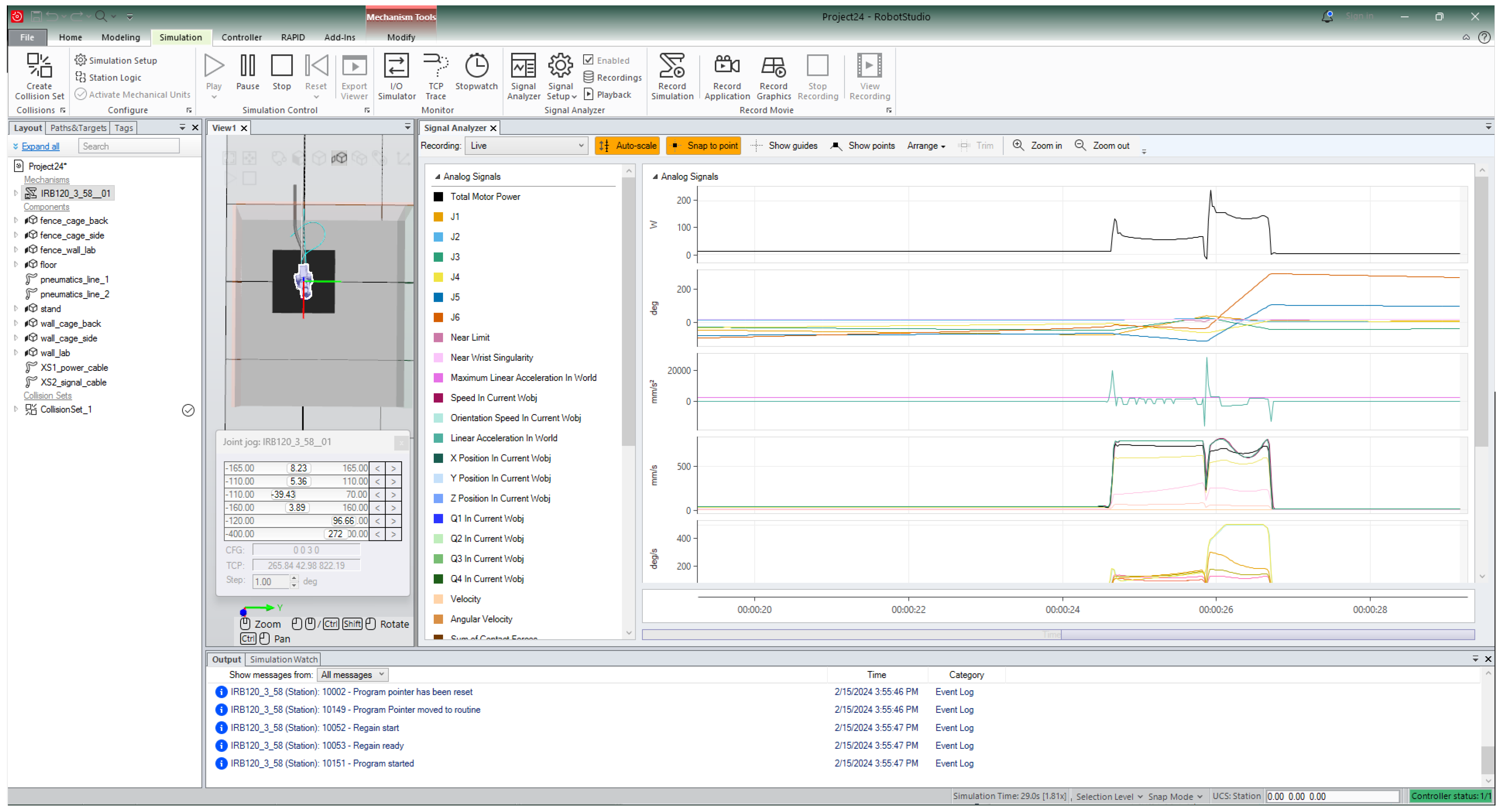
After connecting to the robot and uploading the RAPID code, the simulation in the RobotStudio software package is set up to measure different values. The values measured during the robot movement are:
  • total Motor Power,
  • for each of the joints (J1–J6):
    position in degrees,
    linear velocity,
    angular velocity, and
  • At the end effector:
    linear speed,
    orientation speed,
    linear acceleration,
    position:
    X,
    Y, and
    Z,
    orientation:
    Q1,
    Q2,
    Q3, and
    Q4,
    nearness of limit, and
    nearness of wrist singularity.
To set up RobotStudio to measure the listed values, the first step is to connect the computer running the software package to the control unit of the robot. Then, the code is executed, and the measurement is performed. This appearance of this measurement in RobotStudio can be seen in the Figure 2.
The sampling frequency of the measurement is f s = 40 Hz. Over approximately 1 h and 22 min, this process collected a dataset of 132,192 data points. The simulation time may vary depending on randomly selected speeds of the robot movement. These values, a list of which was given previously, are then exported to a comma-separated value (CSV) file, in such a way that each variable is stored in a separate column. This CSV file will be used for further processing and measurement. The dataset collected in this part of the research is made publicly available [22].

2.1.1. Correlation Analysis

The correlation analysis is performed between all of the values in the dataset. Pearson’s correlation coefficient is calculated between each of the parameters in the dataset. Between two variable sets x 1 and x 2 of length n, the Pearson correlation coefficient r is calculated as:
r = Σ i = 1 n ( x i 1 x ¯ 1 ) ( x i 2 x ¯ 2 ) Σ i = 1 n ( x i x ¯ ) 2 Σ i = 1 n ( y i y ¯ ) 2 .
Based on the correlation coefficient, the dataset is pruned using the following rule: if an input variable has a correlation coefficient lower than 0.2 to the output variable ‘Total Motor Power’ it is eliminated.

2.1.2. Feature Importance

Feature importance is determined with the random forest (RF) algorithm. RF algorithm creates a large number of weak predictors which attempt to regress the target. The created models are tree-based, and as such they are both simple and analyzable [23]. The analysis of models can be performed using two metrics—the mean decrease in impurity (MDI) and feature permutation (FP). FP tests the change of performance when one of the variables is randomly permuted [24], while MDI measures the change of result quality when the feature is added or removed [25]. Based on the results of the feature importance, the dataset is pruned from variables if the MDI or FP value is lower than 0.01.
MDI is calculated according to the impurity. If y i is the value of the output, then I can be calculated per:
I = 1 n i = 1 n ( y i 1 n i = 1 n y i ) 2 .
The MDI is calculated by observing I of the tree model before the variable is included in the model, and I after it was added in the model. Then, the difference Δ I = I I is calculated. The more important the variable is in the modeling of the output, the greater its decrease of impurity should be after the inclusion in the model. FP is calculated by training the dataset normally and noting the R 2 score of the model. Then, one of the variables is randomly shuffled, and the training is performed again. The performance of the two models—one trained on the original dataset, and one trained on the dataset with a single variable randomly shuffled is compared. If the variable is important then the score should decrease significantly, while if the variable has a low influence on the output the score should not change significantly.
In addition to the described techniques for dataset feature preprocessing, several other techniques can be used to remove features with a low influence on the output. One of the main benefits of the applied RF method, which is a tree-based method is that the method provides a simple list of variables that have a low influence and may be removed, allowing for an easy application in conjunction with correlation-based analysis. Decomposition methods are also commonly applied by researchers, such as the principle component analysis (PCA) methods which serve to transform the dataset into a set of principal components [26,27]. Compared to the used approach, the PCA approach does not provide a clear list of variables to be removed (or simply not collected), but the transformation needs to be performed every time new data is collected, before using the developed regression model, possibly adding time to the very fast prediction time of the developed MLP [28]. A more direct approach would be the application of Lasso or Ridge regression to determine the coefficients of the variables and lower them to zero to eliminate the low-influenced ones from the dataset [29]. Still, RF does have some benefits in comparison to these methods such as robustness to non-linearity and multicollinearity, lower sensitivity to outliers and unscaled features, and automatic variable interaction capturing [30,31].

2.2. Regression Methodology

The dataset regression is performed using the MLP method. As stated in the introduction, the goal of using a regression technique instead of an LSTM or similar approaches is the ability to perform the modeling of the instantaneous power. In other words, the authors want to establish a model which will be able to predict the motor power of the industrial robot at any moment—with this prediction being based on the other measured variables such as speed and position, and not the previous values of motor power, as this may enable different optimization schemes. While many regression techniques could have been applied to a dataset of this type authors have selected MLP based on two features, and those are the high performance in similar modeling tasks in the previous research [1] and a high computational speed of the trained models. MLP is constructed from neurons, arranged in layers. Each neuron sums the values of the neurons in the previous layer, multiplied by the values of the weighted connections. These connection weights are values that are updated during the training process [32]. In the training process, the output value—which is the value of the single neuron in the last layer (so-called output neuron), is compared to the expected output for a set of inputs. The error of this prediction is then backpropagated—adjusting weights based on the error gradient in the direction from the output neuron to the input neurons. By repeating this process for each of the data points, over multiple training iterations, the model parameters (weights) are tuned to minimize the error [33].
In addition to the parameters, the neural network also has the so-called hyperparameters. These values describe the initial model of the network, regardless of the trained parameters. These parameters include the number of layers in the network and the number of neurons per layer. In addition, they include the learning rate value and adjustment type which control how quickly are the parameters of the network adjusted during the backpropagation, the activation function of the neurons which is the function that controls the individual neuron output, the regularization parameter which controls the influence of individual variables, and the solver—the algorithm used for recalculating the weights [34]. Hyperparameter tuning is key to obtaining a high-performing dataset, as hyperparameters have a great influence on the model performance [35]. To determine the best set of parameters the grid search procedure is used in this research. First, a set of discrete values is selected for each of the hyperparameters, based on previous research targeting similar topics [1]. These values are given in Table 3. Then, the MLP is trained for each of the possible combinations of hyperparameters. Results are evaluated for each to determine the performance, as it’s described below.
Two separate sets of MLPs are trained in this research. Both target the total motor power of the industrial robotic manipulator, but one attempts to regress it with the entire collected dataset (30 inputs), and the second attempts to regress it with the dataset pruned according to the rules given in the previous section, the results of which are discussed in the following section.
The final structure of the model will consist of the neurons arranged in three types of layers—the input layer, one or more hidden layers, and an output layer. Out of these layers, the simplest one to define is the output layer. This layer will consist of a single neuron. The value of this neuron will represent the predicted value for a given set of inputs, as determined by the forward propagation through the hidden layers. As for the hidden layers, their size will depend on the grid search procedure. As the grid search procedure attempts to tune both the number of hidden layers (between one and five) and the number of neurons in all of the selected layers (selected as 2 n for n [ 0 , 7 ] ), the size of hidden layers can vary between a single layer with one neuron at the smallest and five layers with 128 neurons at the largest. This means that the smallest model would consist of | | x | | + 1 parameters—where | | x | | is the size of the input vector and the + 1 comes from the connection to the output layer. The largest model on the other hand would consist of I + H + O parameters, where I = | | x | | · 128 (connection of the input layer to the first layer), H = 4 × 128 2 (connections between all neurons of one hidden layer to the next), and finally O = 128 (connections of the last hidden layer to the output layer). In other words, this is 128 · | | x | | + 65,664 parameters. The input layer can also vary in size, between two values. This is due to the dataset pruning which is described in the following section. This means that, for the original dataset, the size of the input layer is equal to 30. This means that for it, the model ranges in size from 31 to 69,504 parameters. For the pruned dataset, the input layer is shortened to 15 elements, as shown in the following sections, making its total model parameters range from 16 to 67,584.

Regression Model Evaluation

Each of the models trained in the grid search procedure is subjected to the process of five-fold cross-validation. This process is performed to ensure that the data is not overfitted, and the model generalizes well across data [36]—as the model could overfit on a single part of the dataset and falsely provide good performance metrics. This process is performed in the following manner [37]:
1.
Randomly split the dataset into five subsets F i F 1 , F 2 , F 3 , F 4 , F 5 .
2.
For i in the range from 1 to 5:
  • Create a dataset F t r a i n / t e s t consisting of the four folds whose index doesn’t equal i.
  • Split the F t r a i n / t e s t train and test datasets by randomly selecting points in such a way that F t r a i n is 70% of the dataset, and F t e s t is 30% of the dataset.
  • Perform the training procedure using the two datasets and obtain a trained model.
  • Calculate the performance indexes on the fold F i which was not used in the training set and save them.
3.
Calculate the mean score and the standard deviation of the performance indexes across all folds.
This means that for each of the possible combinations of hyperparameters, the model is trained five times, each time using a different part of the dataset for validation. In each of these five iterations, 74,028 data points are used as the training set ( F t r a i n ), and 18,507 points are used as the test set ( F t e s t ) during training, with results validated on the 39,657 data points. As mentioned, each of these folds is evaluated by using two separate performance indexes—coefficient of determination R 2 and mean absolute percentage error M A P E . These values were selected because they are commonly used in the evaluation of regression models, with R 2 evaluating how well the predicted data follow the trends of the original data across different outputs [38,39], and M A P E defines the absolute difference between the predicted data and the real data across different inputs [40,41]. These two values are utilized because individually they may not provide a good picture of model performance—e.g., a model that has a good variance prediction but a large error will have a good R 2 and a poor M A P E , while the model which follows the data closely, but without taking the trends across inputs into account will demonstrate the opposite.
As mentioned R 2 demonstrates the amount of variance of the original dataset Y = [ y 1 , y 2 , , y N ] contained in the predicted dataset Y ^ = [ y 1 ^ , y 2 ^ , , y N ^ ] [42]. It ranges between [ 0 , 1 ] , where 1 indicates the entirety of variance being contained in the predictions. The higher values of R 2 indicate a higher regression quality. R 2 is defined as:
R 2 = 1 i = 0 N ( y i y ^ i k ) i = 0 N ( y i y ¯ i k ) .
R 2 will provide good scores for models that follow the variance, i.e., the trends contained in the data. But to better express the absolute error of predicted points an error metric should be used. M A P E was selected, as it performs similarly to a popular M A E , but defines the absolute error expressed as a percentage which makes it more straightforward to interpret [43]. It ranges from [ 0 , 100 ] , with the lower values indicating a better regression model. It is calculated per [44]:
M A P E = 1 n Σ i = 0 N | y i y ^ i k y i | .

3. Results

The results will be presented and discussed in this section. First, the results of the metrics for dataset pruning will be considered, as these are needed to prune the dataset for MLP training. Then the results of the models will be presented—with the hyperparameters of the best models given, along with the comparison of the scores between models trained on pruned and original datasets.

3.1. Dataset Pruning Results

The MDI, FP, and r values calculated for the dataset are given in Table 4. If MDI is observed, according to the rules given in the methodology the following variables would be eliminated: speed, X, Y, Z, Q1, Q2, Q3, Q4, Near Limit, Near Singularity, J1, J2, J3, J4, J5, J6, J1 velocity, and angular speed, J3 velocity, and finally J4 velocity and angular speed. Values that are eliminated according to FP are similar, although some values that were eliminated by MDI were kept by FP—namely speed, J4 angular velocity, and J1 angular velocity. The values that would be eliminated according to FP are X, Y, Z, Q1, Q2, Q3, Q4, Near Limit, Near Singularity, J1, J2, J3, J4, J5, J6, J1 velocity, J3 velocity, and finally J4 velocity. Finally, the Pearson’s correlation coefficient can be observed, with the following values showing a lower correlation: linear acceleration, X, Y, Z, Q1, Q2, Q3, Q4, Near Limit, Near Singularity, J1, J2, J3, J4, J5, and J6.
Only those variables that were noted as unimportant by all three sets of methods used for feature importance were removed from the dataset. According to this, the following values are eliminated: X, Y, Z, Q1, Q2, Q3, Q4, Near Limit, Near Wrist Singularity, J1, J2, J3, J4, J5, J6. For easier understanding, the data in Table 4, is visualized in the Figure 3. Here, the stark difference in the influence of positional values compared to the dynamic values connected to the speed of the industrial robotic manipulator is easily visible.
Notably, all of the eliminated values have to do with the positioning of the robotic manipulator. The joint positions J1 through J6 are in fact kinematically connected to the position in tool-space (X, Y, and Z position and orientations Q1–Q4). The same can be said for the information of closeness to limit and singularity. These values having low importance and correlation to an output such as motor power make sense, as they are not dynamic properties.

3.2. Regression Results

The scores for regression are given in Table 5. The scores are given for the complete dataset and the pruned dataset, for both metrics. Scores are given for each of the trained folds, with the average value and standard deviation ( σ ) calculated. Minimum and maximum values are also separated. For the completed dataset, the best average R 2 score is 0.98876, with M A P E of 0.49895. This was achieved by a neural network consisting of five layers with 128 neurons, an adaptive learning rate of 0.0001, a ReLU activation function, and a regularization factor of 0.1. The pruned dataset achieves better results with the same methods—with an average R 2 of 0.99904 and M A P E of 0.33589. Not only are these values lower they are achieved with a smaller neural network of five layers, but with 64 neurons in each layer instead of 128. The network used the same activation function and learning rate as the one used on the original dataset. The smaller network implies that the second problem was simpler to regress, as the network needed fewer parameters to model it. Another notable difference is the value of the regularization factor, which is smaller in the case of the pruned dataset at 0.001. This implies that the first network attempted to lower the influence of variables with higher influence, probably because the parameters that were kept in the pruned dataset had a much higher influence on the output. This was unnecessary in the case of the pruned dataset, as those values are eliminated, and as such the influence of variables does not need to be adjusted by the network during training.
One of the key issues with the application of any pre-processing to ML-based modeling is the issue of increased time and computational complexity added to the modeling process. A benefit of the pre-processing approach to dataset pruning is that it is completed in advance. Compared to the application of methods such as PCA the variable selection is performed in advance. All the future modeling can be based on the subset of variables collected, which can even simplify the dataset collection and processing due to the smaller dataset size (notably, the not-pruned dataset is 33.38 MB in size, while the pruned dataset is 11.00 MB in size—a 67% decrease in size. When it comes to the preprocessing time that is additionally taken up by the dataset pruning, the average time needed for the application of all three feature importance methods (RF with FP and MDI, and Pearson’s correlation) was 4 min and 11 s, with the standard deviation of 9 s. It should be noted that the analyzed dataset is very large, and the modeling was performed on a desktop computer with an Core(™) i5-6400 CPU, manufactured by Intel, Santa Clara, California, USA (six cores and six logical processors, base clocked at 2.9 GHz), and 32 GB of RAM. Scikit-learn Python library [34] was used to determine the feature importances based on RF, while Pandas Python library [45] was used to calculate the correlation. Considering that the MLP models took approximately two days of training on a workstation consisting of an Epyc 7532 processor, manufactured by AMD, Santa Clara, California, USA (24 cores and 48 threads, base clock of 2.3 GHz) and 128 GB of RAM, the time added by the processing of the dataset using feature importance analysis is practically negligible. Considering the possible benefits (lower model complexity, lower training time, a smaller dataset, and most importantly improved scores with the same method), it can be concluded that there is a clear advantage to the application of the suggested method.
The score comparison is apparent in the Figure 4. Not only is the a difference in scores, with pruned achieving better scores—higher for R 2 and lower for M A P E . But also, the pruned dataset shows a better generalization performance. The standard deviation across folds is 0.0007 for pruned and 0.00081 for original datasets considering R 2 metric, and 0.00955 versus 0.05636 considering M A P E . This is apparent in ranges between maximum and minimal values as well. For pruned the difference between the maximum and minimum R 2 score is 0.00020, compared to 0.00228 for the original dataset. For M A P E , the difference between the maximum and minimal score is 0.02916 for the pruned dataset and 0.16318. It can be seen that the differences across folds are a whole magnitude lower for the pruned dataset in comparison to the complete dataset. All of this points towards the fact that pruning the dataset of static values which had a low feature importance causes not only a better performing model but a better generalizing one. Even not taking the generalization performance across folds, the minimum value of the best model is higher than the maximal value for R 2 and lower than the minimal for M A P E —making the performance of the pruned dataset-based model on the worst fold better than the performance of the complete dataset-based set on its best-performing fold.
Comparing the results to the ones achieved by the previous researchers, as shown in Table 1, the applied methodology achieves significantly better results, when the average scores are observed, with an improvement of almost 3% when MAPE is observed and 0.02 increase in the R 2 score. As the improvement is present even when the focus is given to the minimal scores, it can be concluded that the given method of using regression techniques instead of focussing on time-series modeling has a definite merit. The same holds true when the additional validation is performed on different simulated robots as shown in the following section.

3.3. Validation of Results on Different Industrial Robotic Manipulators

To further validate the obtained results, the authors have evaluated different industrial robotic manipulators in a simulated environment. The simulated environment was chosen, due to lack of access to similar robots to the authors. It has to be noted that this process has some limitations—for example, any simulated measurements will not include any noise that may appear during the process of measurement on the real industrial robotic manipulator. Additionally, a real industrial manipulator may have certain influences which affect its motor power use—such as the environment temperature, or the component condition, which are not included within a simulated environment. Despite this, the measurement should be similar enough that a prediction can be established. The process of performing the measurement is done in much the same way as the original data collection. The main change lies in the fact that there is no connection to the robot controller. Instead, an internal virtual controller, included in the ABB RobotStudio [20] is used to control the robot and simulate the measurement. The code used to generate the simulation points is the same, except the limits of the robots are adjusted to reflect the limits provided by the manufacturer in the technical documentation and reference of each robot used for validation—as there are no potential collision points with the environment (e.g., fences, cables, pneumatic lines…) that exist in the real laboratory environment. The robots selected were: IRB 1010, IRB 1100, IRB 1200, IRB 1410, IRB 2600, IRB 4600, IRB 5710. The comparison between the robots is given in Figure 5 The robots were selected as ones having the same virtual controller and overall configuration of joints and degrees-of-freedom as ABB IRB 120—in other words, robots capable of providing the same measurements, with multiple different sizes of robots selected.
Due to this being validation, only ten random points were selected for the database, resulting in datasets that ranged between 300 and 400 individual data points. The measurement was performed only on the variables remaining after the pruning, according to the previously presented methodology. Then, the prediction was performed using the best-performing MLP model given in the previous subsection. The average R 2 and M A P E were calculated between the simulated Total Motor Power and the predicted one, and given in Table 6, below. In the table, the results for IRB 120 are shown both on the separate validation set collected in the laboratory environment and within the simulation.
The results show that there is a significant drop in performance between the real and simulated IRB 120 robot data, with the MAPE increasing from 0.33 to 0.70—more than doubling. Other robots used in the validation procedure also show drops in performance. With the error increasing the more different the robot configuration is (this is mostly addressing the size of the robot). Interestingly, the IRB 1100, which is the ABB replacement for IRB 120 has the lowest error, after the simulated IRB 120. All the other robots, even though the error is increased, still fall within a satisfactory range for M A P E and R 2 . For simplicity, the data is also visually represented in Figure 6.

4. Conclusions

In the presented work a dataset was collected using an ABB IRB 120 industrial robotic manipulator. The dataset in question measured a multitude of quantities related to the position and the speed of the industrial robotic manipulator during the movement. This dataset was analyzed using RF feature importance metrics—MDI and FP and Pearson’s correlation coefficient. Then, variables that had a low significance according to these features were eliminated. An MLP was trained using both the full dataset and the pruned dataset.
The evaluation shows that the model trained on the pruned dataset achieves higher scores compared to the one trained on the original dataset. Comparing the scores, pruning the dataset shows the improvement in the average R 2 score of 0.01128 and the average M A P E score of 0.13306 . The achieved results are better than the results achieved by similar past research focused on using different network types, proving that regression may be a useful approach to this type of modeling, as opposed to using time-series modeling. In addition to this observing standard deviations and minimum/maximum scores across folds shows a better generalization performance for the model trained on the pruned dataset. Based on this, the following conclusions are apparent: (RQ1) A data-driven model with high performance can be developed using the dataset created in this process. (RQ2) Some of the features, namely the static features describing the position of the robotic manipulator in the joint and tool spaces, have a significantly lower influence on the output when analyzed using RF feature importance analysis and Pearson’s correlation coefficient. (RQ3) Not only does the elimination of the variables with lower influence not hurt the performance, but this process also improves the performance across all metrics and subsets used in evaluation, with a smaller neural network.
A limitation of the presented paper is the use of a single industrial robotic manipulator for the dataset creation. Shuffling together data sourced from multiple different manipulators could show a better generalizing model, that could be more securely applied to the power use prediction of different robots. Due to the complexity and cost of accessing multiple industrial robots for these measurements, this research was kept to a single robot—but in the future, based on the positive results it could be expanded to multiple robots using the same methodology. This could serve to improve the performance of the model on different industrial robotic manipulators, as the validation shows a significant drop in performance between models. Future work should also focus on the application of more advanced regression techniques to test if the results could be improved, even without resorting to feature importance-based pruning.

Author Contributions

Conceptualization, S.B.Š. and N.A.; methodology, S.B.Š.; software, S.B.Š.; validation, J.Š. and Z.C.; formal analysis, Z.C.; investigation, J.Š.; resources, Z.C.; data curation, S.B.Š. and N.A.; writing—original draft preparation, S.B.Š.; writing—review and editing, N.A., J.Š. and Z.C.; visualization, J.Š.; supervision, Z.C.; project administration, Z.C. and N.A.; funding acquisition, N.A. and Z.C. All authors have read and agreed to the published version of the manuscript.

Funding

This research has been (partly) supported by the CEEPUS network CIII-HR-0108, the Erasmus+ project WICT, under the grant 2021-1-HR01-KA220-HED-000031177; the University of Rijeka, under scientific grants uniri-tehnic-18-275-1447 and uniri-mladi-technic-22-61.

Data Availability Statement

The original data presented in the study are made openly available by the authors in “Robot Motor Power Dataset” at https://doi.org/10.34740/KAGGLE/DSV/7874548.

Conflicts of Interest

The authors declare no conflicts of interest. The funders had no role in the design of the study; in the collection, analyses, or interpretation of data; in the writing of the manuscript; or in the decision to publish the results.

Abbreviations

The following abbreviations are used in this manuscript:
MLPMultilayer Perceptron
MLMachine Learning
RFRandom Forest
MDIMean Decrease in Impurity
FPFeature Permutation

References

  1. Baressi Šegota, S.; Anđelić, N.; Šercer, M.; Meštrić, H. Dynamics Modeling of Industrial Robotic Manipulators: A Machine Learning Approach Based on Synthetic Data. Mathematics 2022, 10, 1174. [Google Scholar] [CrossRef]
  2. Zhang, H.; Zhang, Y.; Yang, T. A survey of energy-efficient motion planning for wheeled mobile robots. Ind. Robot. Int. J. Robot. Res. Appl. 2020, 47, 607–621. [Google Scholar] [CrossRef]
  3. Farooq, M.U.; Eizad, A.; Bae, H.K. Power solutions for autonomous mobile robots: A survey. Robot. Auton. Syst. 2023, 159, 104285. [Google Scholar] [CrossRef]
  4. Bern, J.M.; Schnider, Y.; Banzet, P.; Kumar, N.; Coros, S. Soft robot control with a learned differentiable model. In Proceedings of the 2020 3rd IEEE International Conference on Soft Robotics (RoboSoft), New Haven, CT, USA, 15 May–15 July 2020; pp. 417–423. [Google Scholar]
  5. Wang, T.; Zhang, L.; Wang, X. Fault detection for motor drive control system of industrial robots using CNN-LSTM-based observers. CES Trans. Electr. Mach. Syst. 2023, 7, 144–152. [Google Scholar] [CrossRef]
  6. Lin, Y.; Zhao, H.; Ding, H. Real-time path correction of industrial robots in machining of large-scale components based on model and data hybrid drive. Robot. Comput.-Integr. Manuf. 2023, 79, 102447. [Google Scholar] [CrossRef]
  7. Benotsmane, R.; Kovács, G. Optimization of energy consumption of industrial robots using classical PID and MPC controllers. Energies 2023, 16, 3499. [Google Scholar] [CrossRef]
  8. Al-Tameemi, M.I.; Hasan, A.A.; Oleiwi, B.K. Design and implementation monitoring robotic system based on you only look once model using deep learning technique. IAES Int. J. Artif. Intell. 2023, 12, 106. [Google Scholar] [CrossRef]
  9. Baressi Šegota, S.; Anđelić, N.; Lorencin, I.; Saga, M.; Car, Z. Path planning optimization of six-degree-of-freedom robotic manipulators using evolutionary algorithms. Int. J. Adv. Robot. Syst. 2020, 17, 1729881420908076. [Google Scholar] [CrossRef]
  10. Kudela, J.; Juříček, M.; Parak, R. A Collection of Robotics Problems for Benchmarking Evolutionary Computation Methods. In Proceedings of the International Conference on the Applications of Evolutionary Computation (Part of EvoStar), Brno, Czech Republic, 12 April 2023; Springer: Berlin/Heidelberg, Germany, 2023; pp. 364–379. [Google Scholar]
  11. Jaramillo-Morales, M.F.; Dogru, S.; Gomez-Mendoza, J.B.; Marques, L. Energy estimation for differential drive mobile robots on straight and rotational trajectories. Int. J. Adv. Robot. Syst. 2020, 17, 1729881420909654. [Google Scholar] [CrossRef]
  12. Jiang, P.; Wang, Z.; Li, X.; Wang, X.V.; Yang, B.; Zheng, J. Energy consumption prediction and optimization of industrial robots based on LSTM. J. Manuf. Syst. 2023, 70, 137–148. [Google Scholar] [CrossRef]
  13. Lin, H.I.; Mandal, R.; Wibowo, F.S. BN-LSTM-based energy consumption modeling approach for an industrial robot manipulator. Robot. Comput.-Integr. Manuf. 2024, 85, 102629. [Google Scholar] [CrossRef]
  14. Huang, K.C.; Yang, H.H.; Chen, W.T. Multi-Scale Aggregation with Self-Attention Network for Modeling Electrical Motor Dynamics. In Proceedings of the 2021 IEEE/RSJ International Conference on Intelligent Robots and Systems (IROS), Prague, Czech Republic, 27 September–1 October 2021; pp. 7097–7103. [Google Scholar]
  15. Kontopoulou, V.I.; Panagopoulos, A.D.; Kakkos, I.; Matsopoulos, G.K. A review of ARIMA vs. machine learning approaches for time series forecasting in data driven networks. Future Internet 2023, 15, 255. [Google Scholar] [CrossRef]
  16. Moein, M.M.; Saradar, A.; Rahmati, K.; Mousavinejad, S.H.G.; Bristow, J.; Aramali, V.; Karakouzian, M. Predictive models for concrete properties using machine learning and deep learning approaches: A review. J. Build. Eng. 2023, 63, 105444. [Google Scholar] [CrossRef]
  17. Šegota, S.B.; Anđelić, N.; Mrzljak, V.; Lorencin, I.; Kuric, I.; Car, Z. Utilization of multilayer perceptron for determining the inverse kinematics of an industrial robotic manipulator. Int. J. Adv. Robot. Syst. 2021, 18, 1729881420925283. [Google Scholar] [CrossRef]
  18. Husnain, A.; Rasool, S.; Saeed, A.; Hussain, H.K. Revolutionizing Pharmaceutical Research: Harnessing Machine Learning for a Paradigm Shift in Drug Discovery. Int. J. Multidiscip. Sci. Arts 2023, 2, 149–157. [Google Scholar] [CrossRef]
  19. ABB Ltd. ABB IRB 120 3/0.6 Product Manual; ABB Ltd.: Zurich, Switzerland, 2022. [Google Scholar]
  20. ABB Ltd. Operating Manual RobotStudio; ABB Ltd.: Zurich, Switzerland, 2022. [Google Scholar]
  21. ABB Ltd. Technical Reference Manual—RAPID Instructions, Functions and Data Types; ABB Ltd.: Zurich, Switzerland, 2022. [Google Scholar]
  22. Baressi Šegota, S. Robot Motor Power Dataset. 2024. Available online: https://www.kaggle.com/datasets/sandibaressiegota/robot-motor-power-dataset (accessed on 27 March 2024).
  23. Sevšek, L.; Šegota, S.B.; Car, Z.; Pepelnjak, T. Determining the influence and correlation for parameters of flexible forming using the random forest method. Appl. Soft Comput. 2023, 144, 110497. [Google Scholar] [CrossRef]
  24. Molnar, C.; Freiesleben, T.; König, G.; Herbinger, J.; Reisinger, T.; Casalicchio, G.; Wright, M.N.; Bischl, B. Relating the partial dependence plot and permutation feature importance to the data generating process. In Proceedings of the World Conference on Explainable Artificial Intelligence, Lisbon, Portugal, 26–28 July 2023; Springer: Berlin/Heidelberg, Germany, 2023; pp. 456–479. [Google Scholar]
  25. Scornet, E. Trees, forests, and impurity-based variable importance in regression. Ann. L’Institut Henri Poincare (B) Probab. Stat. 2023, 59, 21–52. [Google Scholar] [CrossRef]
  26. Gárate-Escamila, A.K.; El Hassani, A.H.; Andrès, E. Classification models for heart disease prediction using feature selection and PCA. Inform. Med. Unlocked 2020, 19, 100330. [Google Scholar] [CrossRef]
  27. Anđelić, N.; Baressi Šegota, S. Development of symbolic expressions ensemble for breast cancer type classification using genetic programming symbolic classifier and decision tree classifier. Cancers 2023, 15, 3411. [Google Scholar] [CrossRef]
  28. Gu, J.; Hua, W.; Yu, W.; Zhang, Z.; Zhang, H. Surrogate model-based multiobjective optimization of high-speed PM synchronous machine: Construction and comparison. IEEE Trans. Transp. Electrif. 2022, 9, 678–688. [Google Scholar] [CrossRef]
  29. Fahimifar, S.; Mousavi, K.; Mozaffari, F.; Ausloos, M. Identification of the most important external features of highly cited scholarly papers through 3 (ie, Ridge, Lasso, and Boruta) feature selection data mining methods: Identification of the most important external features of highly cited scholarly papers through 3 (ie, Ridge, Lasso, and Boruta) feature selection data mining methods. Qual. Quant. 2023, 57, 3685–3712. [Google Scholar]
  30. Afrin, S.; Shamrat, F.J.M.; Nibir, T.I.; Muntasim, M.F.; Moharram, M.S.; Imran, M.; Abdulla, M. Supervised machine learning based liver disease prediction approach with LASSO feature selection. Bull. Electr. Eng. Inform. 2021, 10, 3369–3376. [Google Scholar] [CrossRef]
  31. Yang, X.; Wen, W. Ridge and lasso regression models for cross-version defect prediction. IEEE Trans. Reliab. 2018, 67, 885–896. [Google Scholar] [CrossRef]
  32. Afzal, S.; Ziapour, B.M.; Shokri, A.; Shakibi, H.; Sobhani, B. Building energy consumption prediction using multilayer perceptron neural network-assisted models; comparison of different optimization algorithms. Energy 2023, 282, 128446. [Google Scholar] [CrossRef]
  33. Xu, Y.; Li, F.; Asgari, A. Prediction and optimization of heating and cooling loads in a residential building based on multi-layer perceptron neural network and different optimization algorithms. Energy 2022, 240, 122692. [Google Scholar] [CrossRef]
  34. Pedregosa, F.; Varoquaux, G.; Gramfort, A.; Michel, V.; Thirion, B.; Grisel, O.; Blondel, M.; Prettenhofer, P.; Weiss, R.; Dubourg, V.; et al. Scikit-learn: Machine learning in Python. J. Mach. Learn. Res. 2011, 12, 2825–2830. [Google Scholar]
  35. Almeida, L.B. Multilayer perceptrons. In Handbook of Neural Computation; CRC Press: Boca Raton, FL, USA, 2020; p. C1–2. [Google Scholar]
  36. de Rooij, M.; Weeda, W. Cross-validation: A method every psychologist should know. Adv. Methods Pract. Psychol. Sci. 2020, 3, 248–263. [Google Scholar] [CrossRef]
  37. Xiong, Z.; Cui, Y.; Liu, Z.; Zhao, Y.; Hu, M.; Hu, J. Evaluating explorative prediction power of machine learning algorithms for materials discovery using k-fold forward cross-validation. Comput. Mater. Sci. 2020, 171, 109203. [Google Scholar] [CrossRef]
  38. Chen, G.; Muriki, H.; Sharkey, A.; Pradalier, C.; Chen, Y.; Dellaert, F. A Hybrid Cable-Driven Robot for Non-Destructive Leafy Plant Monitoring and Mass Estimation using Structure from Motion. In Proceedings of the 2023 IEEE International Conference on Robotics and Automation (ICRA), London, UK, 29 May–2 June 2023; pp. 11809–11816. [Google Scholar]
  39. Meattini, R.; Caporali, A.; Bernardini, A.; Palli, G.; Melchiorri, C. Self-Supervised Regression Of sEMG Signals Combining Non-Negative Matrix Factorization with Deep Neural Networks for Robot Hand Multiple Grasping Motion Control. IEEE Robot. Autom. Lett. 2023, 8, 8533–8540. [Google Scholar] [CrossRef]
  40. Peng, F.; Lu, Y.; Wang, Y.; Yang, L.; Yang, Z.; Li, H. Predicting the formation of disinfection by-products using multiple linear and machine learning regression. J. Environ. Chem. Eng. 2023, 11, 110612. [Google Scholar] [CrossRef]
  41. Efendi, S.; Nasution, M.K.; Herman, M. The Role of Detection Rate in MAPE to Improve Measurement Accuracy for Predicting FinTech Data in Various Regressions. In Proceedings of the 2023 International Conference on Computer Science, Information Technology and Engineering (ICCoSITE), Jakarta, Indonesia, 16 February 2023; pp. 874–879. [Google Scholar]
  42. Chicco, D.; Warrens, M.J.; Jurman, G. The coefficient of determination R-squared is more informative than SMAPE, MAE, MAPE, MSE and RMSE in regression analysis evaluation. PeerJ Comput. Sci. 2021, 7, e623. [Google Scholar] [CrossRef]
  43. Wang, Y.Q.; Wang, H.C.; Song, Y.P.; Zhou, S.Q.; Li, Q.N.; Liang, B.; Liu, W.Z.; Zhao, Y.W.; Wang, A.J. Machine learning framework for intelligent aeration control in wastewater treatment plants: Automatic feature engineering based on variation sliding layer. Water Res. 2023, 246, 120676. [Google Scholar] [CrossRef] [PubMed]
  44. Li, C.; Cheang, B.; Luo, Z.; Lim, A. An exponential factorization machine with percentage error minimization to retail sales forecasting. ACM Trans. Knowl. Discov. Data (TKDD) 2021, 15, 1–32. [Google Scholar] [CrossRef]
  45. McKinney, W.; Team, P. Pandas-Powerful python data analysis toolkit. Pandas—Powerful Python Data Anal. Toolkit 2015, 1625. [Google Scholar] [CrossRef]
Figure 1. The IRB 120 industrial robotic manipulator used for measurements.
Machines 12 00225 g001
Figure 2. The measurement data collected in the RobotStudio software, prior to CSV export.
Machines 12 00225 g002
Figure 3. The visualization of variable influences on the output.
Machines 12 00225 g003
Figure 4. Graphical comparison of scores between two datasets.
Machines 12 00225 g004
Figure 5. The robots used in the validation — in order from left to right: IRB 1010, IRB 120, IRB 1100, IRB 1200, IRB 1410, IRB2600, IRB 4600, IRB 5710.
Machines 12 00225 g005
Figure 6. Comparison of validation results across different robots.
Machines 12 00225 g006
Table 1. The best results demonstrated in relevant previous studies.
PaperScore
Jaramillo-Morales et al. [11] R 2 = 0.97 %
Jian et al. [12] M A P E = 4.21 %
Lin et al. [13] M A P E = 3.67 %
Huang et al. [14] M A P E = 3.30 %
Table 2. The lower and upper limits of joints used in the simulation.
Joint iLower Limit l i [deg]Higher Limit h i [deg]
1−9090
2−1045
3−10040
4−160160
5−120120
6−400400
Table 3. The hyperparameters used in the grid search.
HyperparameterPossible ValuesCount
Number of layers1, 2, 3, 4, 55
Number of neurons1, 2, 4, 8, 16, 32, 63, 1288
ActivationReLU, Identity, Logistic, Tanh4
SolverAdam, LBFGS2
Learning rate typeConstant, Adaptive, Inverse Scaling3
Initial learning rate0.5, 0.1, 0.01, 0.001, 0.0001, 0.000016
L2 regularization0.1, 0.01, 0.001, 0.00014
Table 4. The feature importance metrics calculated on the dataset.
VariableMDIFPr
Speed0.0066330.0228680.864878
Orientation Speed0.0155120.062970.786160
Linear Acceleration0.0184310.013540.100195
X0.0031130.0022590.015793
Y0.0042710.0024720.004599
Z0.0049530.0059730.006784
Q10.0016890.000749−0.008261
Q20.002850.001533−0.012481
Q30.0020230.0008230.005319
Q40.0019470.0007310.005534
Near Limit0.0009530.0005340.023404
Near Wrist Singularity0.0004640.000076−0.031361
J1 Position0.0058470.0028960.009030
J2 Position0.0039840.00390.012479
J3 Position0.003370.002305−0.012455
J4 Position0.0038760.003745−0.082532
J5 Position0.0047410.004204−0.019140
J6 Position0.0044880.003533−0.002446
J1 Velocity0.005090.0083280.869247
J1 Angular Velocity0.0069350.0136660.869241
J2 Velocity0.0114750.0128080.842528
J2 Angular Velocity0.027470.0246380.892606
J3 Velocity0.0044540.0087340.842867
J3 Angular Velocity0.6124070.3874110.905022
J4 Velocity0.0057420.0043140.880788
J4 Angular Velocity0.0092640.015360.853524
J5 Velocity0.0854470.0422040.884634
J5 Angular Velocity0.0177170.0152530.859018
J6 Velocity0.0206850.0165910.882829
J6 Angular Velocity0.1041680.0391640.793835
Table 5. The scores for best-performing models on pruned and complete datasets, per each fold, with calculated average and standard deviation across folds, as well as minimal and maximum values separated.
DatasetMetricFoldAVG σ MINMAX
12345
Pruned R 2 0.999350.999290.999220.999210.999150.999240.000070.999150.99935
M A P E 0.324320.334420.333790.333430.353490.335890.009550.324310.35349
Complete R 2 0.989530.987920.987660.987440.987250.987960.000810.987250.98953
M A P E 0.411370.469540.574540.433790.455490.468950.056360.411360.57454
Table 6. The validation results on the simulation data, per robot.
Robot R 2 MAPE
IRB 120-laboratory0.995380.34914
IRB 120-simulation0.989430.70443
IRB 10100.976580.93569
IRB 11000.980140.81644
IRB 12000.972130.97089
IRB 14100.970251.01027
IRB 26000.951341.11287
IRB 46000.953451.23064
IRB 57100.951521.26427
Disclaimer/Publisher’s Note: The statements, opinions and data contained in all publications are solely those of the individual author(s) and contributor(s) and not of MDPI and/or the editor(s). MDPI and/or the editor(s) disclaim responsibility for any injury to people or property resulting from any ideas, methods, instructions or products referred to in the content.

