Improved PVTOL Test Bench for the Study of Over-Actuated Tilt-Rotor Propulsion Systems

Abstract

In recent years, applications exploiting the advantages of tilt-rotors and other vectored thrust propulsion systems have become widespread, particularly in many novel Vertical Takeoff and Landing (VTOL) configurations. These propulsion systems can provide additional control authority, enabling more complex flight modes, but the resulting control systems can be challenging to design due to the mismatch between the vehicle degrees of freedom and physical input variables. These propulsion systems present both advantages and difficulties because they can exert the same overall forces and moments in many different propulsive configurations. This leads to the traditional non-uniqueness problem when using the inverse dynamics control allocation approach, which is the basis of many popular VTOL control algorithms. In this article, a modified Planar VTOL (PVTOL) test bench configuration, which considers an arbitrary number of co-linear tilting rotors, is introduced as a benchmark for the study of the control allocation problem. The resulting propulsion system is then modeled and linearized in a closed and compact form. This allows a simple and systematic derivation of many of the currently used control allocation approaches. According to the proposed PVTOL configuration, a two-rotor test bench is implemented experimentally and a decoupling control allocation strategy based on Singular Value Decomposition (SVD) analysis is developed. The proposed approach is compared with a traditional input mixer algorithm based on physical intuition. The results show that the SVD-based solution achieves better cross-coupling reduction and preserves the main properties of the physically derived approach. Finally, it is shown that the proposed PVTOL configuration is effective for studying the control allocation problem experimentally in a controlled environment and could serve as a benchmark for comparing different approaches.

1. Introduction

Recently, Vertical Takeoff and Landing (VTOL) aircraft configurations have attracted a high degree of interest from the research community and the aeronautics industry. The novelty of these vehicles introduces a set of challenging issues because many of the well-established design methodologies, used for conventional aircraft configurations, do not apply directly. This has also attracted the attention of the authorities, which have proposed several novel specifications to address many of these challenges (see, for example, [1,2]).

The majority of the reports found in the literature deal with a specific VTOL configuration. For instance, in [3,4], the authors study a commonly used arrangement, in which the tilt-rotors are used to generate either lift force in hover or thrust force in horizontal flight (i.e., as the one used in the V-22 Osprey). In this case, the authors propose a nonlinear observer and control approach to stabilize the vehicle with good results. Many other aspects of this configuration have been researched, for instance, in [5], the dynamic properties of the vehicle are studied by calculating the linear stability and control derivatives of the vehicle. This study shows that it is possible to evaluate the well-known flight modes of a traditional airplane such as phugoid, short period, Dutch roll, and spiral subsidence. Using a similar approach. In [6], it is shown that a linear control approach can be used to stabilize the full nonlinear dynamics of the vehicle. In this case, the authors noticed a serious degree of cross-coupling when the vehicle operated in helicopter mode. A similar configuration, which considers that the aircraft remains in hover with a vertical fuselage orientation, is studied in [7]. In this report, the authors used a scheduled linear control approach to stabilize the vehicle. These reports show that, although this VTOL configuration results in a highly coupled and nonlinear system, the use of linear control approaches is preferred in some instances due to its simplicity and the possibility of evaluating the closed loop dynamics in terms of classical flight dynamics modes.

Although the configuration mentioned in the previous paragraph is common, it is far from being the only one used in VTOL applications. In particular, tilt-rotors can be found in several configurations, ranging from all the rotors being tilt-rotors to a single rotor used as a tilt-rotor. For instance, in [8], a fixed-wing aircraft with one fixed and two tilting rotors is presented. In this case, a set of nested control loops with linear controllers is used to stabilize the vehicle. Several reviews dealing with VTOL configurations can be found in the literature [9,10,11]. From these reports, the following insights can be obtained:

• There is a high degree of heterogeneity in the propulsion system configurations, including number, distribution, and operating conditions.
• There is an increasing use of distributed tilting rotors (or similar thrust vectoring elements).
• The multiplicity of propulsors and control surfaces results in a high number of control inputs, introducing an over-actuation problem, which is normally denoted as the control allocation problem in the literature (although under-actuation problems have also been treated as allocation problems by some authors).
• The control allocation problem is commonly dealt with by separating the vehicle into two parts: (1) a rigid body, which is driven by virtual control inputs (i.e., force and moment vectors), and (2) the propulsion subsystem, which is driven in such a way that the desired force and moment vectors are obtained. In practice, it is difficult to pair specific physical inputs to a particular force or moment component without introducing cross-coupling in the rigid body control loop.
• Although many control approaches have been proposed, linear Proportional Integral Derivative (PID) controllers are still used in many practical setups due to their simplicity and low computational overhead.

The control allocation problem is one of the main issues found in novel vehicle configurations with many tilting propulsors. The simplest approach for the allocation problem consists of pairing specific physical inputs with the desired outputs in a fully decentralized control manner. In other cases, physical insight allows proposing a simple allocation strategy [8]. Although these approaches have been used for traditional configurations (i.e., classical pairings, such as elevator surface and pitch angle), many novel VTOL configurations cannot be operated using this scheme due to excessive cross-coupling.

In cases where the cross-coupling introduced by a simple control allocation algorithm is excessive, a preferred approach consists of establishing virtual (decoupled) inputs and attempting to solve the inverse actuator dynamics to determine the necessary physical inputs [9]. This approach is easy and effective if the propulsion subsystem inverse dynamics exist and are unique. A well-known example of this is the typical quad-rotor control allocation algorithm, where a vector of four virtual inputs is related to the angular velocities of the four propellers through a fixed and invertible 4x4 matrix [12]. It is also interesting to note that this approach has proven to be highly successful even though the propulsion model used to derive it is arguably over-simplified, as it neglects several important aerodynamic factors [13]. This proves that it is possible to obtain effective allocation solutions using simplified propulsion models.

In more recent years, VTOL configurations have become more complex so that inverse propulsion dynamics either do not exist or are not unique. In particular, over-actuated systems are more common due to the increased number of actuators. In these cases, a simple solution consists of using physical insights to add additional constraints to reduce the dimension of the control input vector. For example, in [14], the control allocation for a spacecraft using two kinds of actuators was solved by a proportional distribution of the desired control torque considering the characteristics of each actuator. Physical insight has also been used to refine Cascade-Generalized Inversion (CGI) approaches, such as in [15], where a test bench for a vehicle with multiple tilting rotors was controlled by grouping several physical actuators in a hierarchical manner. There are also several mathematical tools which can aid in solving the allocation problem, such as the Moore–Penrose pseudo-inverse matrix and the Karush–Kuhn–Tucker (KKT) optimality conditions [16]. Many of these approaches rely on a linear approximation approach, whose range can be expanded by the use of scheduling techniques [16]. Non-linear approaches have been also proposed; however, the resulting solutions can be too taxing for the computational systems on board small vehicles. Therefore, fast linear or scheduling approaches are still preferred in many applications [16,17].

More recently, in [17], a review article dealing with the taxonomy of vehicles with multiple rotors showed that there are still many challenges in the study of these propulsion systems. Among these, the heterogeneity of the propulsion configurations, the aerodynamic interaction of the various actuators (also noted in [13]), and the actuator limitations (including actuator saturation and response times) are the most relevant. One of the tools observed in [17] which has been used to overcome some of these problems is the use of co-linear or co-planar propulsor arrangements.

The previous paragraphs illustrate how the popularization of VTOL vehicles with a wide range of configurations, particularly those that contain an arbitrary number of tilting rotors, has motivated the study of the control allocation problem, from both theoretical and practical points of view. In this context, it is appropriate to recall that during the emergence of the modern quad-copter drone, in the early 2000s and later, several novel technical and theoretical developments were made. One of the tools that proved to be very valuable for researchers was the so called Planar Vertical Takeoff and Landing (PVTOL) configuration, which was widely adopted by researchers in a simplified two degrees of freedom (DoF) test bench version. This simplified model allowed both researchers and prospective control engineers to study novel control strategies and to perform preliminary experimental tests in a safe environment before performing actual flight tests. The sheer number of contributions to control, sensor, and modelling theory that still rely on the PVTOL configuration is a testament to its usefulness. From neural network backstepping control [18] to the study of robust feedback linearization [19] and noise-rejecting active disturbance controllers [20], the PVTOL model is still widely used by researchers. In many ways, the PVTOL has become a de facto benchmark platform.

While the PVTOL is a good approximation of simple vehicles such as the quad-copter, this simplification fails to capture the main difficulties of many current VTOL vehicles. In particular, many of these vehicles include some form of tilt-rotor or other similar thrust vectoring propulsion system. There have been some attempts to propose a more general PVTOL configuration, which also include the complications of tilting rotors. For example, in [21], a tilting rotor PVTOL was introduced with good results; however, in this report, only simulations are presented and the allocation problem is reduced by neglecting the reactive torque of the propellers.

Finally, a summary of the main elements found in the literature review is as follows:

• There is a high level of heterogeneity in the propulsion configuration of recent VTOL vehicles with a movement towards a higher number of actuators.
• The resulting control allocation problems are highly dependent on the propulsion configuration. Therefore, the study of this issue can yield vehicle-specific results.
• The use of simplified test benches (such as the PVTOL) can aid in the study of prospective control strategies while preserving many of the dynamic and experimental complexities, allowing a more rapid development of novel/better solutions.
• The typical PVTOL test bench configuration is unable to represent many of the difficulties found in recent VTOL vehicles.
• Although non-linear control and allocation approaches can deliver improved performance for wider operating ranges, in many Unmanned Aerial Vehicle (UAV) applications, linear controllers and allocation approaches are still being used and researched due to their simplicity and efficiency.

Considering the previous context, in this article, the control allocation problem is studied both theoretically and experimentally. In particular, the following elements are presented:

• A novel PVTOL test bench configuration containing an arbitrary number of co-linear tilting rotors is proposed as a progression of the traditional PVTOL test bench configuration. This configuration can reproduce several of the interesting issues found in novel VTOL vehicles, mainly the control allocation and cross-coupling problems. In addition, this configuration can be easily extended to include an arbitrary number of co-planar tilting propulsors, so that a wider range of vehicles can be mimicked.
• A general method for obtaining a closed form of the linearization of the propulsion model for the modified PVTOL configuration is presented. This can be useful because, as mentioned before, many control allocation strategies depend on it.
• A simple test bench, based on the modified PVTOL configuration, is implemented experimentally. This simple test bench allows testing control allocation and cross-coupling problems.
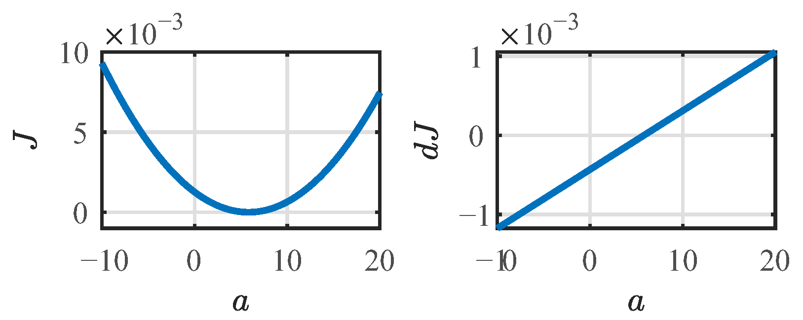
• A simple decoupling control allocation scheme for the test bench, based on a linear approximation derived through Singular Value Decomposition (SVD), is presented. This approach allows defining an optimal solution for the allocation problem of the modified PVTOL configuration. The resulting optimization can solve the over-actuation problem by introducing a wide range of considerations. In this case, low-error and practical physical considerations are used.
• The proposed SVD control allocation approach is compared with a more traditional input mixer algorithm, derived from physical insight, both through simulations and using the experimental test bench. The results show that the proposed control allocation scheme allows decreasing the cross-coupling with a simple static decoupling matrix.

The authors also want to emphasize that the test bench presented here (as well as the proposed allocation algorithm) should be considered an initial step towards a generalized study of the control allocation problem through the use of a prospective standardized test bench configuration based on the modified PVTOL configuration. The authors believe that the proposed test bench could be used by the scientific community for this purpose; however, those seeking additional complexity may consider adding more co-linear propulsors (or even co-planar propulsors in an arbitrary matrix configuration). This would result in an even more complex over-actuation problem. The authors hope that the use of such a family of test benches could potentially become a widely used benchmark as an aid in the study and development of novel propulsion systems for VTOL vehicles.

2. Materials and Methods

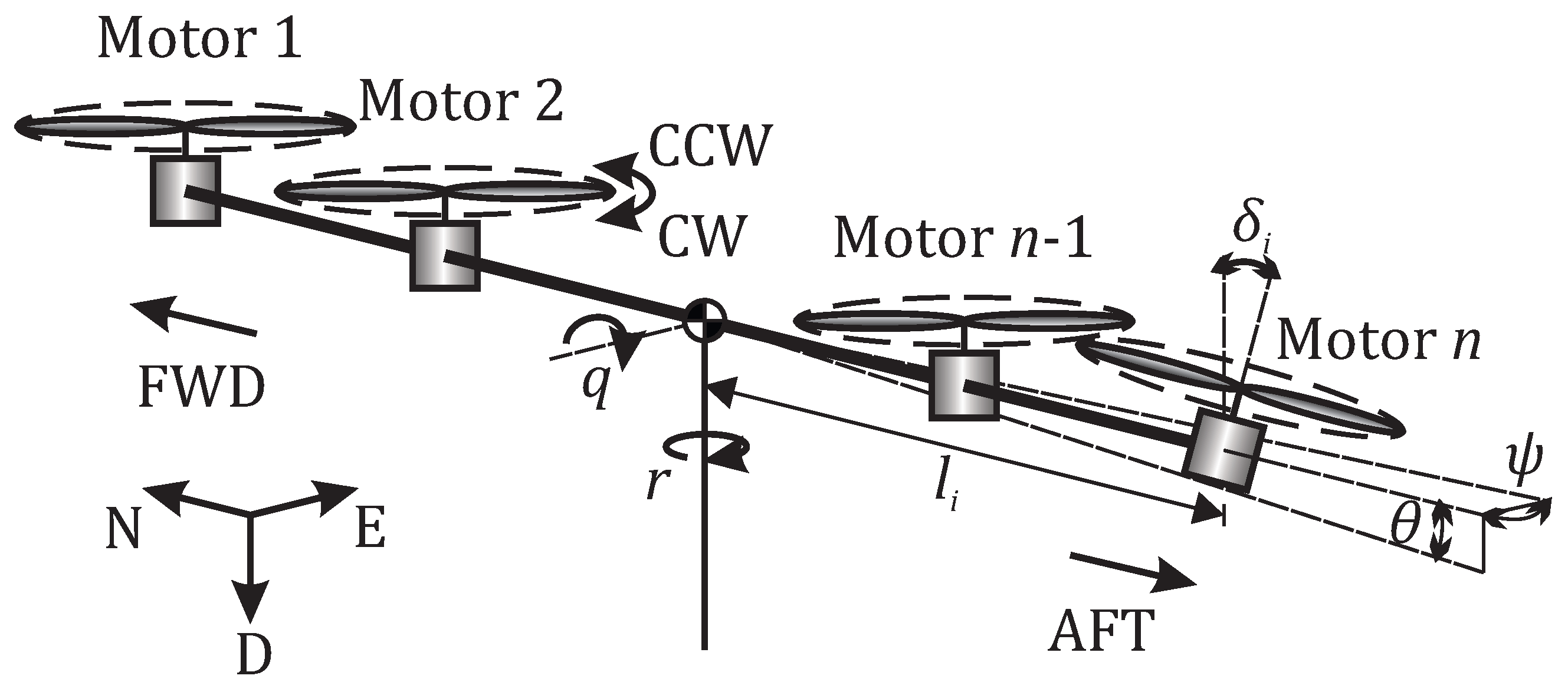
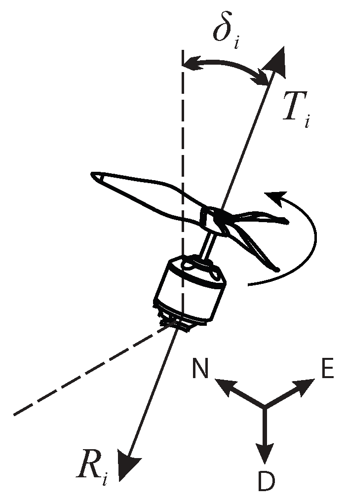
2.1. A PVTOL with an Arbitrary Number of Co-Linear Tilting Rotors

This section introduces a PVTOL test bench with an arbitrary number of co-linear tilting rotors and derives the linearization of the resulting propulsion system model in a compact and closed form. This propulsion configuration was chosen because it can replicate many of the control allocation problems found in a wide range of vehicles and can be easily extended to a more complex arbitrary co-planar propulsion system by simple aggregation. In comparison with the typical PVTOL experimental test bench configuration, which is restricted to a single DoF (pitch angle), the proposed configuration adds yaw angle as an additional DoF. This enables the introduction of a multivariable control problem (i.e., two outputs instead of one), which facilitates a better study of the control allocation problem.

It must be noted that adding further DoFs to the test bench (for example, roll angle) could increase its research potential at the cost of increased mechanical complexity. In this regard, it is important to recognize that a successful test bench benchmark must balance the trade-off between its mechanical/manufacturing complexity and its research value potential. To support this claim, consider the classical PVTOL test bench, which is normally restricted to pitch angle movement. Although this restriction is clearly not completely representative of vehicles such as the quad-copter, as mentioned in the introduction, this has not precluded the classical PVTOL test bench from being used for a wide range of studies related to quad-rotor applications. In this case, the proposed configuration remains simple enough to be cost- and mechanically accessible, but complex enough for the control allocation and multivariable cross-coupling problems to appear. Therefore, we believe that the proposed configuration (in particular, the two-rotor version presented in an upcoming section) represents a similar sweet spot for these problems, as the classical PVTOL test bench is for the typical quad-rotor.

Figure 1 shows the propulsion system with an arbitrary number (n) of tilting rotors, where the distance of each rotor from the center of gravity is denoted by $l_i$ and the tilt angle of each rotor is denoted by ${\delta }_i$, with $i=1,2,3,\dots n$. The figure also depicts the angular positions and rates of the PVTOL in a typical inertial North-East-Down (NED) reference frame, where $\theta$ and $\psi$ denote the pitch and yaw angles, respectively, and q and r denote the pitch and yaw rates, respectively.

Each motor/propeller induces a thrust force $T_i$ and a moment $R_i$ aligned with its tilt angle, as shown in Figure 2. Because $R_i$ is produced by rotational drag, its direction is opposite to the propeller rotation. According to simplified propeller modelling, typically used for multi-rotor vehicles, force $T_i$ and moment $R_i$ can be modelled as [13]:

$$\begin{array}{c}{T}_i=\frac{1}{2}\rho S{C}_T{{\omega }_i}^2\hfill \\ R_i=\frac{1}{2}\rho S{C}_Q{{\omega }_i}^2\hfill \end{array}$$

(1)

where S is the disc area of the propeller, $C_T$ is the thrust coefficient, $C_Q$ is the reactive moment coefficient, $\rho$ is the air density, and ${\omega }_i$ is the angular speed of propeller i. Accordingly, $R_i$ can be rewritten as $R_i=k_i{T}_i$ with $k_i=C_Q/C_T$, which is convenient to reduce the number of independent input variables.

This article studies the control allocation problem for the pitching and yawing moments, denoted as M and N, respectively, since these are the two natural degrees of freedom for a test bench with the modified PVTOL configuration of Figure 1. Following this configuration, the resulting pitching and yawing moments are:

$$\begin{array}{c}M={\displaystyle \sum _{i=1}^n}{T}_i{l}_{i}cos{\delta }_i{(-1)}^{{\alpha }_i}-{\displaystyle \sum _{i=1}^n}{T}_i{k}_{i}sin{\delta }_i{(-1)}^{{\beta }_i}\hfill \\ N={\displaystyle \sum _{i=1}^n}{T}_i{k}_{i}cos{\delta }_i{(-1)}^{{\beta }_i}+{\displaystyle \sum _{i=1}^n}{T}_i{l}_{i}sin{\delta }_i{(-1)}^{{\alpha }_i}\hfill \end{array}$$

(2)

with:

$${\alpha }_i=\left\{\begin{array}{cc}0,\hfill & \mathrm{if}\mathrm{position}\mathrm{FWD}\hfill \\ 1,\hfill & \mathrm{if}\mathrm{position}\mathrm{aft}\hfill \end{array}\right.$$

(3)

$${\beta }_i=\left\{\begin{array}{cc}0,\hfill & \mathrm{if}\mathrm{rotation}\mathrm{CCW}\hfill \\ 1,\hfill & \mathrm{if}\mathrm{rotation}\mathrm{CW}\hfill \end{array}\right.$$

(4)

where CW, CCW, and FWD denote clockwise, counterclockwise, and forward respectively.

For instance, considering a simple two-rotor arrangement, with a FWD propeller ($i=1$) rotating CCW and an aft propeller ($i=2$) rotating CW, the resulting moment equations yield:

$$\begin{array}{c}M=T_1{l}_{1}cos{\delta }_1-T_2{l}_{2}cos{\delta }_2-T_1{k}_{1}sin{\delta }_1+T_2{k}_{2}sin{\delta }_2\hfill \\ N=T_1{k}_{1}cos{\delta }_1-T_2{k}_{2}cos{\delta }_2+T_1{l}_{1}sin{\delta }_1-T_2{l}_{2}sin{\delta }_2\hfill \end{array}$$

(5)

Although the non-linear propulsion model given by Equations (2) and (5), is useful for many applications, such as simulation, evaluation, and non-linear control design, many control allocation methods are based on a linear representation of the propulsion subsystem. As follows, the linear approximation of the two-propeller case will be derived and then extended for the general case.

The linear approximation of (5) is given by the Jacobian matrix P of the moment vector ${\left[MN\right]}^T$, that is:

$$\left[\begin{array}{c}\mathsf{\Delta }M\\ \mathsf{\Delta }N\end{array}\right]=P\left[\begin{array}{c}\mathsf{\Delta }{T}_1\\ \mathsf{\Delta }{\delta }_1\\ \mathsf{\Delta }{T}_2\\ \mathsf{\Delta }{\delta }_2\end{array}\right]$$

(6)

with

$$P={\left[\begin{array}{cccc}\frac{\partial M}{\partial T_1}& \frac{\partial M}{\partial {\delta }_1}& \frac{\partial M}{\partial T_2}& \frac{\partial M}{{\delta }_2}\\ \frac{\partial N}{\partial T_1}& \frac{\partial N}{\partial {\delta }_1}& \frac{\partial N}{\partial T_2}& \frac{\partial N}{{\delta }_2}\end{array}\right]}_0$$

(7)

where ${\left[\mathsf{\Delta }M\mathsf{\Delta }N\right]}^T$ and ${\left[\mathsf{\Delta }{T}_1\mathsf{\Delta }{\delta }_1\mathsf{\Delta }{T}_2\mathsf{\Delta }{\delta }_2\right]}^T$ are the resulting linear output and input vectors, and the sub-index 0 denotes evaluation in the equilibrium point.

Matrix P is also called the propulsion matrix in the literature and its properties (e.g., range) are a determining factor when calculating the physical control inputs (i.e., ${\left[T_1{\delta }_1{T}_2{\delta }_2\right]}^T$) necessary to reach a desired combination of input moments (i.e., ${\left[MN\right]}^T$). In this case, since the control inputs vector $\in \mathbb{R}{}^4$, while the moment vector $\in \mathbb{R}{}^2$, this PVTOL configuration yields an over-actuation problem, which will be studied in more detail later in the article.

From (6), it follows that:

$$P={\left[\begin{array}{cccc}{l}_{1}cos{\delta }_1-k_{1}sin{\delta }_1& -T_1{l}_{1}sin{\delta }_1-k_1{T}_{1}cos{\delta }_1& -l_{2}cos{\delta }_2+k_{2}sin{\delta }_2& T_2{l}_{2}sin{\delta }_2+k_2{T}_{2}cos{\delta }_2\\ l_{1}sin{\delta }_1+k_{1}cos{\delta }_1& T_1{l}_{1}cos{\delta }_1-k_1{T}_{1}sin{\delta }_1& -l_{2}sin{\delta }_2-k_{2}cos{\delta }_2& -T_2{l}_{2}cos{\delta }_2+k_2{T}_{2}sin{\delta }_2\end{array}\right]}_0$$

(8)

Matrix P can be further decomposed as:

$$P=A{P}_1=\left[\begin{array}{cccc}{l}_1& -k_1& -l_2& k_2\\ k_1& l_1& -k_2& -l_2\end{array}\right]{\left[\begin{array}{cccc}cos{\delta }_1& -T_{1}sin{\delta }_1& 0& 0\\ sin{\delta }_1& T_{1}cos{\delta }_1& 0& 0\\ 0& 0& cos{\delta }_2& -T_{2}sin{\delta }_2\\ 0& 0& sin{\delta }_2& T_{2}cos{\delta }_2\end{array}\right]}_0$$

(9)

Furthermore, matrix $P_1$ can also be decomposed as:

$$P_1=BC={\left[\begin{array}{cccc}cos{\delta }_1& -sin{\delta }_1& 0& 0\\ sin{\delta }_1& cos{\delta }_1& 0& 0\\ 0& 0& cos{\delta }_2& -sin{\delta }_2\\ 0& 0& sin{\delta }_2& cos{\delta }_2\end{array}\right]}_0{\left[\begin{array}{cccc}1& 0& 0& 0\\ 0& T_1& 0& 0\\ 0& 0& 1& 0\\ 0& 0& 0& T_2\end{array}\right]}_0$$

(10)

Therefore, matrix P can be rewritten as:

$$P=ABC=\left[\begin{array}{cccc}{l}_1& -k_1& -l_2& k_2\\ k_1& l_1& -k_2& -l_2\end{array}\right]{\left[\begin{array}{cccc}cos{\delta }_1& -sin{\delta }_1& 0& 0\\ sin{\delta }_1& cos{\delta }_1& 0& 0\\ 0& 0& cos{\delta }_2& -sin{\delta }_2\\ 0& 0& sin{\delta }_2& cos{\delta }_2\end{array}\right]}_0{\left[\begin{array}{cccc}1& 0& 0& 0\\ 0& T_1& 0& 0\\ 0& 0& 1& 0\\ 0& 0& 0& T_2\end{array}\right]}_0$$

(11)

Following the structure of (11), a generalization for the system with n propulsors can be derived. In particular, following a similar analysis, the linearization of the full non-linear propulsion subsystem (2) is given by:

$$\left[\begin{array}{c}\mathsf{\Delta }M\\ \mathsf{\Delta }N\end{array}\right]=P\left[\begin{array}{c}\mathsf{\Delta }{T}_1\\ \mathsf{\Delta }{\delta }_1\\ ⋮\\ \mathsf{\Delta }{T}_n\\ \mathsf{\Delta }{\delta }_n\end{array}\right]$$

(12)

where $P=ABC$ and $A\in {\mathbb{R}}^{2\times 2n}$, $B\in {\mathbb{R}}^{2n\times 2n}$, and $C\in {\mathbb{R}}^{2n\times 2n}$.

As follows, each of the elements which comprise (12) will be derived in a closed and compact form. First, matrix A, which contains information regarding the location and orientation of each rotor, can be written as the concatenation of sub-matrices $A_i$:

$$A=\left[\begin{array}{cccc}{A}_1& A_2& \cdots & A_{{}_n}\end{array}\right]$$

(13)

with

$$A_{{}_i}=\left[\begin{array}{cc}{l}_i{(-1)}_i^{\alpha }& k_i{(-1)}^{{\beta }_i+1}\\ k_i{(-1)}_i^{\beta }& l_i{(-1)}_i^{\alpha }\end{array}\right]$$

(14)

In addition, B comprises a set of 2D rotation sub-matrices as:

$$B=diag\{B_1,B_2,\dots ,B_n\}$$

(15)

with

$$B_i={\left[\begin{array}{cc}cos{\delta }_i& -sin{\delta }_i\\ sin{\delta }_i& cos{\delta }_i\end{array}\right]}_0$$

(16)

Finally, matrix C contains information regarding the equilibrium thrust of each propeller:

$$C=diag\{C_1,C_2,\cdots ,C_n\}$$

(17)

with

$$C_i={\left[\begin{array}{cc}1& 0\\ 0& T_i\end{array}\right]}_0$$

(18)

This completes the derivation of the linear approximation of the propulsion subsystem of the PVTOL of Figure 1. The structure obtained here is useful because it allows separating the three main physical properties that determine the resulting propulsion matrix P. In particular:

• Matrix A contains information regarding the physical position and rotation direction of each propeller. Since these properties are normally constant, updating matrix A is not necessary when calculating a linear approximation on a different operating point. However, analyzing its structure could be useful to determine which particular propulsive configuration is better for particular applications.
• Matrix B contains information regarding the tilt angle of each of the propellers. Depending on the operating range and behavior of the propulsion system, this matrix could be the most sensible for operating point modifications, and should be updated accordingly in scheduling approaches.
• Matrix C contains information regarding the thrust force of each propeller. This matrix could also require regular updates in a scheduling approach depending on the operating behavior of the vehicle.

In many cases, matrices B and C may not require a full update if only a sub-set of rotors change their operating point. Instead, updating sub-matrices $B_i$ and $C_i$ may be sufficient.

Although, in this case, the derivation and decomposition of the propulsion matrix was performed for the modified PVTOL, it may be possible that a similar decomposition could be useful for other complex propulsion systems, which is the motivation for this analysis (i.e., as a proof of concept).

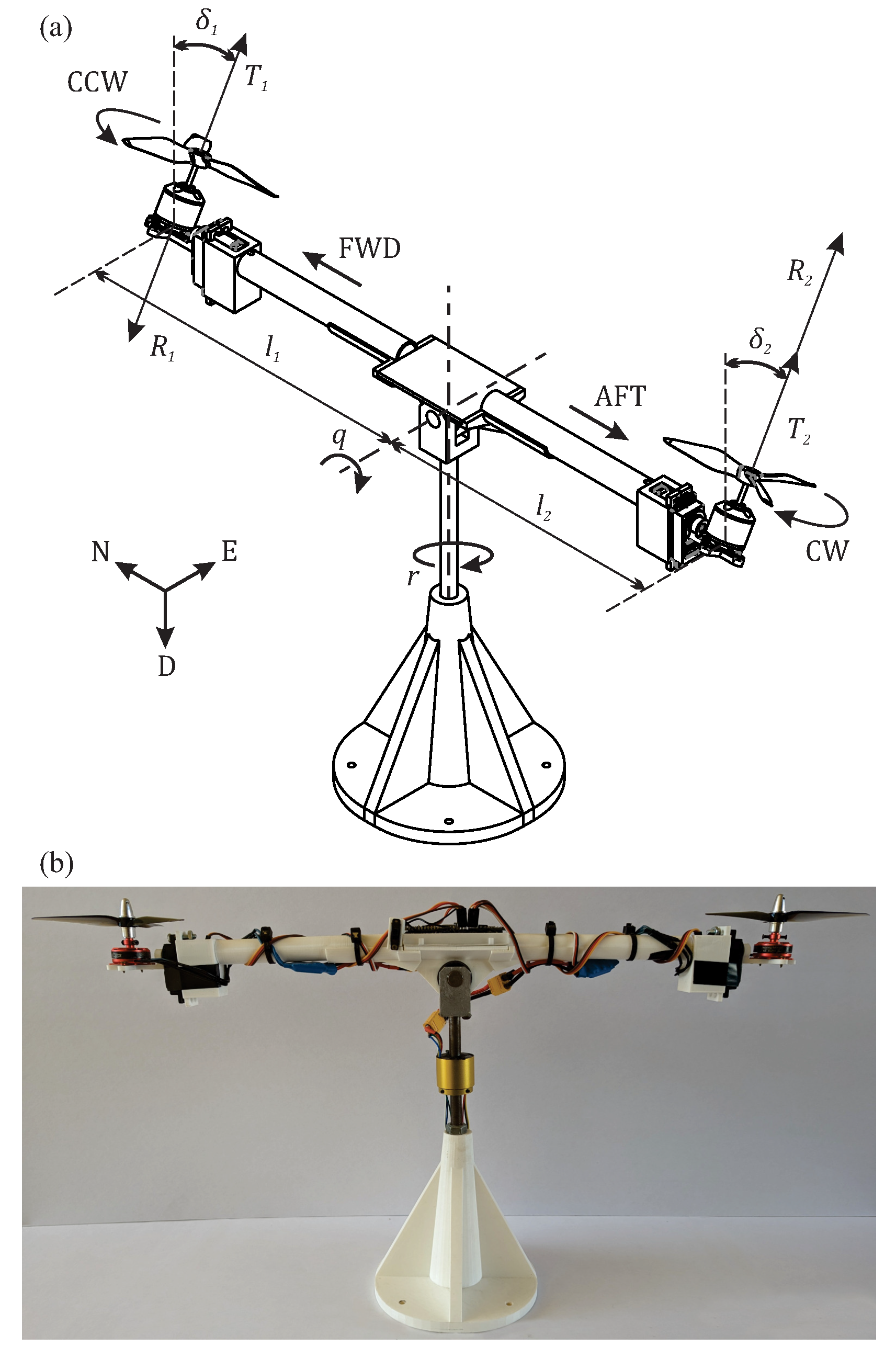
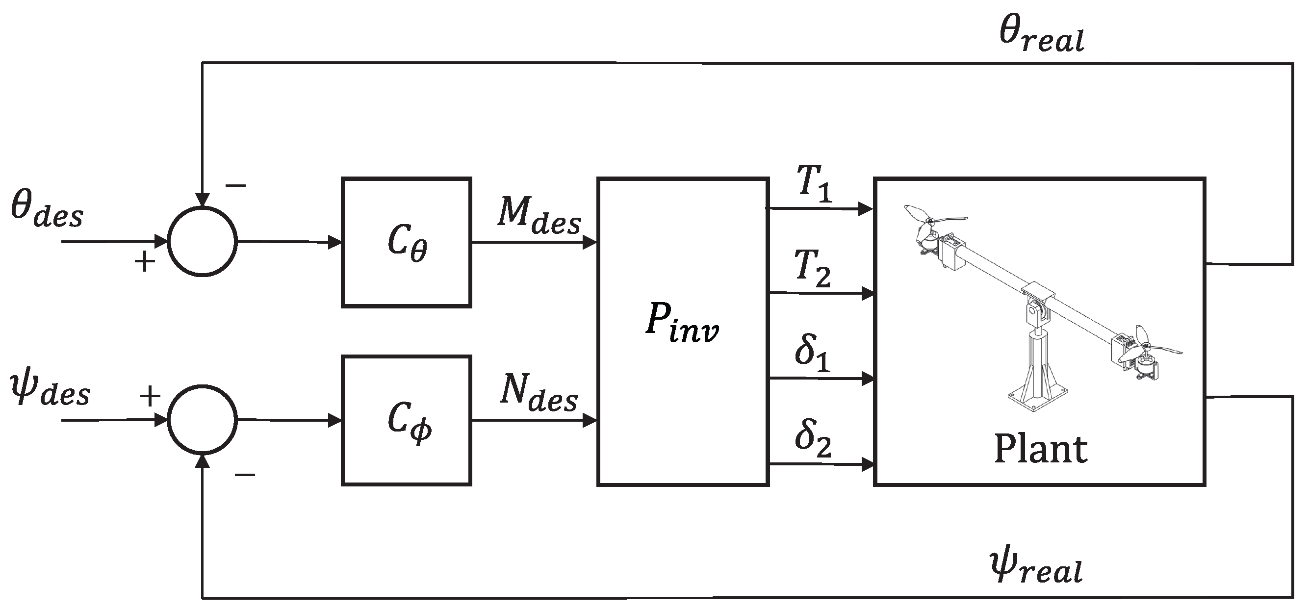
2.2. Experimental Test Bench

In this section, an experimental test bench considering the modified PVTOL configuration proposed in the previous section is introduced. The schematic of the test bench is shown in Figure 3a, while Figure 3b shows the actual prototype. Although this is a simple two-rotor setup, this configuration yields an over-actuated system (as noted in the previous section); thus, it is sufficient to study the control allocation problem.

The test bench consists of a base with a transverse rod connecting a servo-motor at each end. Two bearings allow the system to move freely on two degrees of freedom. Brushless motors with propellers are attached to each of the servo-motors. A summary of the technical specifications of the test bench is as follows:

• Two 2304 Racestar brushless motors (81 W max power).
• Two Gemfan 51466 three-blade propellers, one CW and one CCW.
• Two MG995 servo-motors.
• One BNO055 absolute orientation sensor.

The orientation angles are measured using the BNO055 absolute orientation sensor array, which consists of a 3-axis accelerometer and gyroscope combined with a Kalman filter for the pitch and yaw angle reconstruction. These kinds of sensors are normally able to deliver measurements with a mean error of under 1.5 deg/s and 0.5 m/s${}^2$ for the gyroscope and accelerometer, respectively [22,23,24]. This configuration can yield a low level of angle measurement error in applications where no axial acceleration is present, so that the main source of measured acceleration is the gravity, as in the present application [25].

The test bench was operated with an external power source with a fixed voltage of 12 V, which provided enough current for all the operating conditions tested. The control algorithms were implemented in an ATmega2560 microcontroller, which is a low-power 8-bit micro controller capable of 6 MIPS at 16 MHz. The possibility to implement the proposed control allocation algorithm in this low-computational-power microcontroller is a salient characteristic, since most low-cost autopilot UAV solutions have limited computational power.

The microcontroller code was directly generated with Simulink/Matlab without further optimization operating at a sampling rate of 5 ms. Figure 4 shows the overall Simulink program used for the implementation of the control algorithms presented in this article.

An Atmel-based microcontroller board was programmed for the test bench. A summary of the resulting input and output variables for the test bench is shown next.

• Input variables:

  –

  Right motor thrust $T_1$;

  –

  Left motor thrust $T_2$;

  –

  Tilt angle of right motor ${\delta }_1$;

  –

  Tilt angle of left motor ${\delta }_2$.

• Output variables:

  –

  Pitch rate $\dot{\theta }=q$;

  –

  Yaw rate $\dot{\psi }=r$;

  –

  Pitch angle $\theta$;

  –

  Yaw angle $\psi$.

Further details regarding the experimental and simulation setups are shown in Section 3, together with the corresponding experiments and simulations.

Recalling Equation (5), the resulting motion equations are given by:

$$\begin{array}{c}{I}_{yy}\dot{q}=T_1{l}_{1}cos{\delta }_1-T_2{l}_{2}cos{\delta }_2-T_1{k}_{1}sin{\delta }_1+T_2{k}_{2}sin{\delta }_2\hfill \\ I_{zz}\dot{r}=T_1{k}_{1}cos{\delta }_1-T_2{k}_{2}cos{\delta }_2+T_1{l}_{1}sin{\delta }_1-T_2{l}_{2}sin{\delta }_2\hfill \end{array}$$

(19)

where $I_{yy}$ and $I_{zz}$ are the pitch and yaw inertial masses, respectively.

Accordingly, the resulting model considering the linearized propulsion model yields:

$$\left[\begin{array}{cc}{I}_{yy}& 0\\ 0& I_{zz}\end{array}\right]\left[\begin{array}{c}\mathsf{\Delta }\dot{q}\\ \mathsf{\Delta }\dot{r}\end{array}\right]=P\left[\begin{array}{c}\mathsf{\Delta }{T}_1\\ \mathsf{\Delta }{\delta }_1\\ \mathsf{\Delta }{T}_2\\ \mathsf{\Delta }{\delta }_2\end{array}\right]$$

(20)

with $P\in {\mathbb{R}}^{2\times 4}$ as in Equation (11).

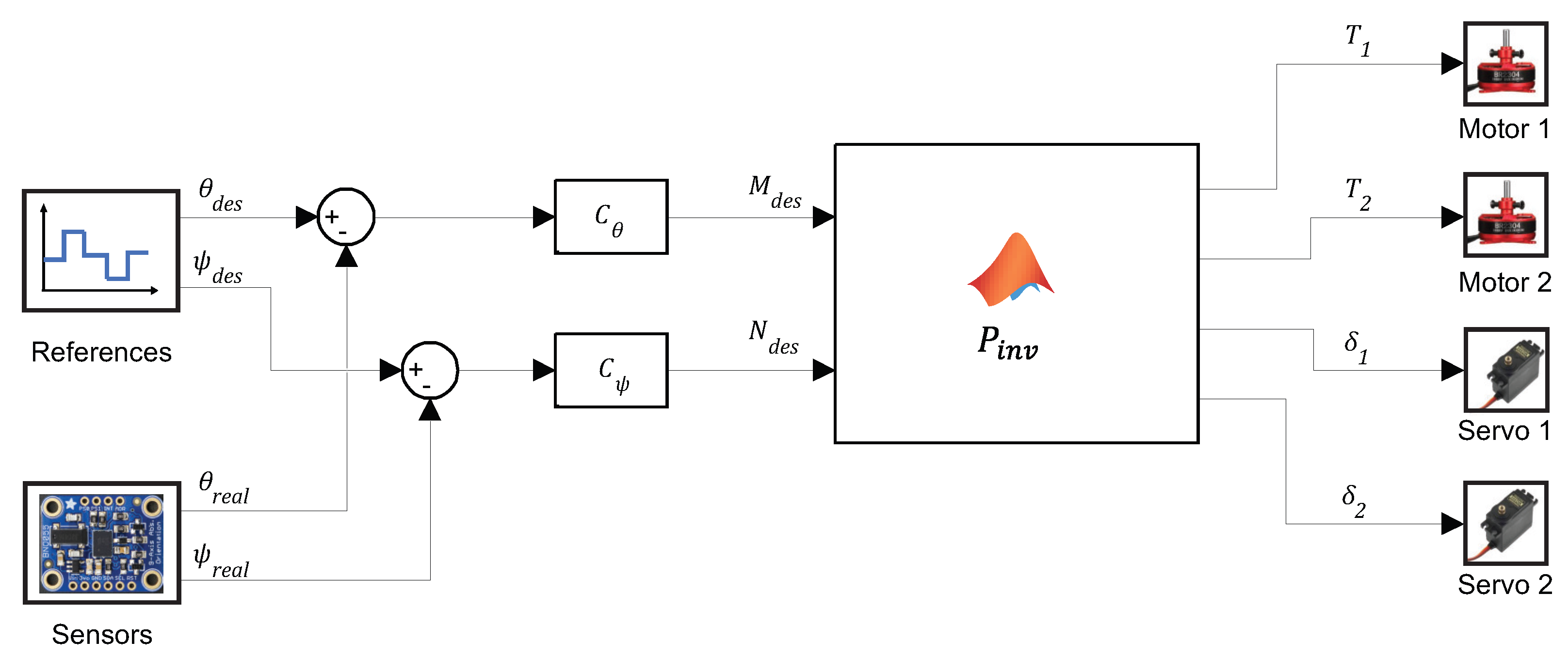
2.3. Control Allocation Problem

The objective is to design a linear controller for the pitch and yaw angles of the test bench using the input vector ${\left[T_1{\delta }_1{T}_2{\delta }_2\right]}^T$. According to (20), this results in an over-actuated and a multivariable control problem. Although there are several control approaches which can deal with multivariable cross-coupling, an ideal approach would be to have an input-decoupling scheme which incorporates two virtual inputs, that is:

$$\left[\begin{array}{cc}{I}_{yy}& 0\\ 0& I_{zz}\end{array}\right]\left[\begin{array}{c}\mathsf{\Delta }\dot{q}\\ \mathsf{\Delta }\dot{r}\end{array}\right]=\left[\begin{array}{c}{M}_{des}\\ N_{des}\end{array}\right]$$

(21)

where $M_{des}$ and $N_{des}$ are the two arbitrary virtual inputs.

Therefore, in this case, the control allocation problem consists in finding a matrix $P_{inv}$ such that $I=P{P}_{inv}$ so that the required physical input variables can be calculated for a particular value of the desired virtual inputs, that is:

$$\left[\begin{array}{c}{T}_1\\ {\delta }_1\\ T_2\\ {\delta }_2\end{array}\right]=P_{inv}\left[\begin{array}{c}{M}_{des}\\ N_{des}\end{array}\right]$$

(22)

In this article, two approaches to solve the control allocation problem will be compared: (1) a decentralized control approach based on physical intuition and (2) a mathematical approach based on SVD and optimization.

2.3.1. Physical Intuition-Based Decentralized Control Allocation

In this section, a proposal for the input signal mixer will be derived based on physical intuition and the following assumptions:

• A decentralized control approach for the pitch and yaw angles is sufficient to stabilize the test bench. This implies that pitch and yaw moments are derived separately without considering their interaction. This normally implies, for instance, that when calculating the pitch angle input mixer (directly related to $M_{des}$), it is assumed that $N_{des}=0$. In addition, if the pitch angle mixer also affects the yawing moment N, then these effects are neglected, or at best considered as input perturbations for the yaw angle controller. That is, any residual cross-coupling is neglected.
• A small range of operation for the tilt-rotors is enough to stabilize the test bench. This assumption allows maintaining the focus of this study on the linear elements of the control allocation problem, which is the basis of most scheduling approaches. Later, it will be confirmed experimentally that indeed only small tilt angles are required for the stabilization of this PVTOL configuration. Nonetheless, extension of these results for wider operating ranges will be forthcoming in future studies.

For small angles, the system tends to behave as a classical PVTOL configuration with a single degree of freedom in the pitch angle and propeller thrust as inputs. In this case, the resulting pitching moment yields:

$$M=l_1{T}_1-l_2{T}_2$$

(23)

Thus, it is reasonable to use the differential thrust of propellers to induce pitching moment. In addition, when no pitching moment is required, it is also desirable for both propellers to maintain a specific equilibrium thrust $T_0$. This yields the well-known PVTOL pitching moment input mixer:

$$T_1=T_0+\frac{M_{des}}{2l_1}{T}_2=T_0-\frac{M_{des}}{2l_2}$$

(24)

On the other hand, in the case of the yaw angle, if $T_1\approx T_2$ (i.e., $M_{des}\approx 0$), then the yawing moment yields:

$$N=T_1\left(k_{1}cos{\delta }_1-k_{2}cos{\delta }_2\right)+T_1\left(l_{1}sin{\delta }_1-l_{2}sin{\delta }_2\right)$$

(25)

Accordingly, noticing that $T_1\approx T_2$ in (24) implies $T_1\approx T_0$, the small angle approximation for the yawing moments is:

$$N=T_0{l}_1{\delta }_1-T_0{l}_2{\delta }_2$$

(26)

Therefore, the input mixer for the yawing moment is proposed as:

$${\delta }_1=\frac{N_{des}}{2T_0{l}_1}{\delta }_2=-\frac{N_{des}}{2T_0{l}_2}$$

(27)

Equations (24) and (27) will be used for the decentralized control allocation approach. It is clear that in this case, the pitching moment is achieved by modifying the propeller thrust, whereas the yawing moment is achieved by modifying the rotor tilt angle. Therefore, this solution is also easy to understand and to implement.

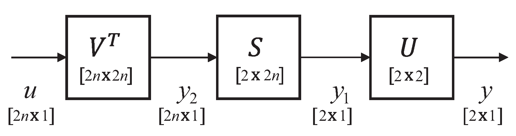
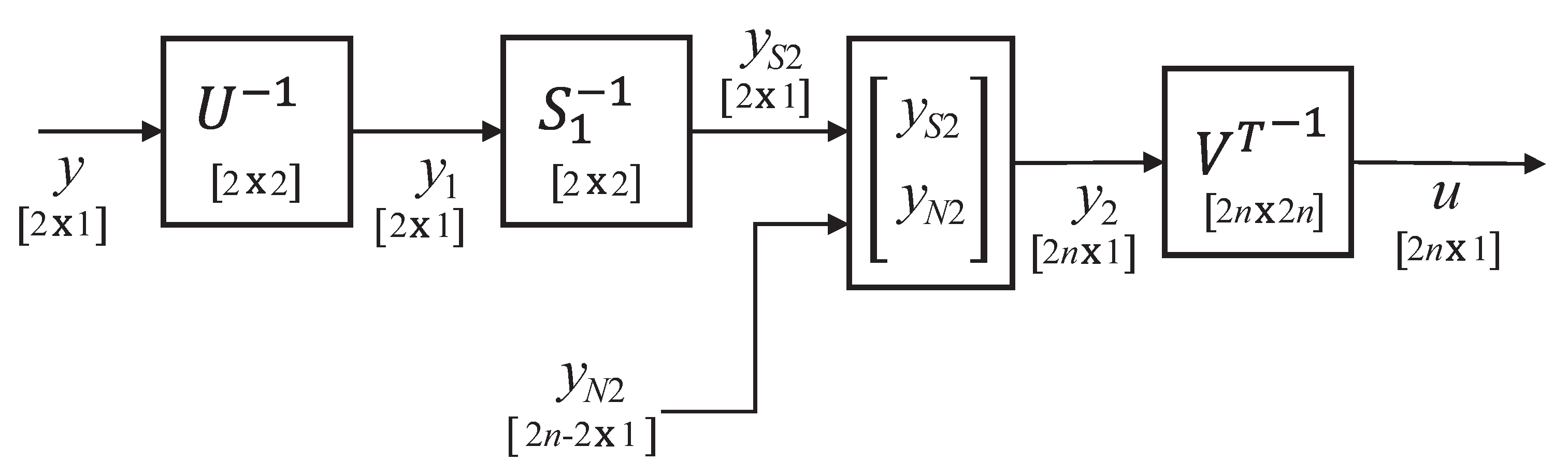
2.3.2. Singular Value Decomposition Control Allocation

In this section, a simple control allocation solution will be derived using the SVD analysis of the linearization of the propulsion system. Recalling Equation (6), the SVD of matrix P yields:

$$P_{2\times 2n}=U_{2\times 2}{S}_{2\times 2n}{V}_{2n\times 2n}^T$$

(28)

where the sub-indexes show the size of each matrix.

Matrix S is a rectangular diagonal matrix called the singular values matrix, whose diagonal elements $s_i$ are always positive, typically written in descending order, and are called the singular values of matrix P. In addition, matrices S and V are orthogonal. The rank of matrix P is equal to the number of non-zero singular values. Thus, matrix P can be considered as a linear transformation of $R^{2n}$ into $R^{r_s}$, where $r_s=rank\left(S\right)$ is the number of non-zero $s_i$ values, which in this case, since $S\in R^{2\times 2n}$, can only be at most 2. Finally, this analysis shows that for the modified PVTOL configuration with arbitrary number of tilting rotors, a fully decoupling control allocation solution exists iff $r_s=2$.

The SVD of matrix P also allows viewing the linear transformation between an input vector $u\in R^{2n}$ and an output vector $y\in R^2$ as a series of intermediate linear transformations, as shown in Figure 5, where the intermediate transformed vectors are $y_2\in R^{2n}$ and $y_1\in R^2$, that is:

$$y_2=V^{T}u{y}_1=S{y}_{2}y=U{y}_1$$

(29)

Figure 5 shows that the loss of dimension introduced by matrix P occurs in the intermediate transformation $y_1=S{y}_2$ and is due to the rank of matrix S. In particular, matrix S has the following structure:

$$S=\left[\begin{array}{cc}{S}_1& 0_{2\times 2n-2}\end{array}\right]$$

(30)

where $0_{2\times n-2}$ denotes a zero matrix of the indicated size and $S_1$ is given by:

$$S_1=diag\{s_1,s_2\}$$

(31)

If the rank of P is two (i.e., $S_1$ is invertible), then all the possible input combinations u which produce a particular desired output y can be calculated with:

$$\begin{array}{c}{y}_1=U^{T}y\hfill \\ y_{2S}={S_1}^{-1}{y}_1\hfill \\ y_2=\left[\begin{array}{c}{y}_{2S}\\ y_{2N}\end{array}\right]\hfill \\ u=V{y}_2\hfill \end{array}$$

(32)

where $y_{2N}\in R^{2n-2}$ is an arbitrary vector which does not have any effect over the resulting output vector y.

If $y_{2N}=0$, then Equation (32) yields the Moore–Penrose pseudo-inverse. In particular, $y_{2N}$ introduces additional degrees of freedom which account for the null subspace of S. The process of using this pseudo-inverse transformation to calculate an input u which produces a particular desired output y is represented in Figure 6. This allows injecting an arbitrary vector $y_{2N}$ which can be selected according to additional practical considerations. Note that in this case, the SVD analysis was preferred over the direct pseudo-inverse approach because of the additional flexibility that the SVD decomposition yields, such as more precise control of the null space injection and information contained in matrices S and V.

2.3.3. SVD-Based Control Allocation Configuration

In the previous section, a control allocation approach based on SVD was presented for the general case of n co-linear tilting rotors. This method introduced additional degrees of freedom which could be potentially used to better comply with additional specifications. In this section, the SVD control allocation method will be applied to the two-rotor modified PVTOL test bench and the additional degrees of freedom will be configured according to practical considerations.

Considering the physical parameters of the test bench, and the equilibrium points reported in

Table 1. Test bench parameters and equilibrium points.

Variable	Value
$T_{1_0}$	$4.12$$\mathrm{N}$
$T_{2_0}$	$4.12$$\mathrm{N}$
${\delta }_{1_0}$	0°
${\delta }_{2_0}$	0°
$l_{1,2}$	$0.205$   $\mathrm{m}$
$k_{1,2}$	$0.0103$   $\mathrm{m}$

, the propulsion matrix P (i.e., the linear approximation of the propulsion system) yields:

$$P=\left[\begin{array}{cccc}0.2050& -0.0424& -0.2050& 0.0424\\ 0.0103& 0.8446& -0.0103& -0.8446\end{array}\right]$$

(33)

Using Equations (28) and (32) with $u={\left[T_1{\delta }_1{T}_2{\delta }_2\right]}^T$ and $y={\left[M_{des}{N}_{des}\right]}^T$ yields:

$$\left[\begin{array}{c}{T}_1\\ {\delta }_1\\ T_2\\ {\delta }_2\end{array}\right]=\left[\begin{array}{cccc}2.433& 0.122& 0.707& -0.025\\ -0.029& 0.592& 0.025& 0.707\\ -2.433& -0.122& 0.707& -0.025\\ 0.029& -0.592& 0.025& 0.707\end{array}\right]\left[\begin{array}{c}{M}_{des}\\ N_{des}\\ a\\ b\end{array}\right]$$

(34)

where the vector containing the additional degrees of freedom is given by $y_{2N}={\left[ab\right]}^T$.

Parameters a and b can be selected freely according to the designer considerations. In this case, the first consideration is that it is desirable that ${\delta }_1={\delta }_2=0$ when $M_{des}=N_{des}=0$. Physically, this implies that, in equilibrium, the rotors should point upwards. Therefore, from (34), it is required that

$$0.025a+0.707b=0$$

(35)

Thus, b is set as:

$$b=-0.035a$$

(36)

Next, parameter a is selected so that the quadratic error considering the non-linear propulsion model is minimized. This yields the following minimization problem:

$$\underset{a}{min}J=(e_M^2+e_N^2)$$

(37)

with:

$$\left[\begin{array}{c}{e}_M\\ e_N\end{array}\right]=\left[\begin{array}{c}M\\ N\end{array}\right]-P{P}_{inv}\left(a\right)\left[\begin{array}{c}{M}_{des}\\ N_{des}\end{array}\right]$$

(38)

where M and N are as in Equation (5), P is from (33), and $P_{inv}\left(a\right)$ is matrix (34) with an arbitrary a value.

A simple numerical exercise, shown graphically in Figure 7, reveals that the optimal value for this parameter is $a=5.82$.

Finally, the resulting input mixer yields:

$$\left[\begin{array}{c}{T}_1\\ {\delta }_1\\ T_2\\ {\delta }_2\end{array}\right]=\left[\begin{array}{c}2.433M_{des}+0.122N_{des}+4.12\\ -0.029M_{des}+0.592N_{des}\\ -2.433M_{des}-0.122N_{des}+4.12\\ 0.029M_{des}-0.592N_{des}\end{array}\right]$$

(39)

2.3.4. Final Mixer Algorithm Comparison

In this section, the resulting mixer algorithms using both approaches will be compared for $T_1$ and ${\delta }_1$ (note that $T_2$ and ${\delta }_2$ are similar). In particular, the decentralized control approach using the parameters of Table 1 and Equations (24) and (27) yields:

$$T_{1,dec}=4.12+2.43M_{des}{\delta }_{,dec}=0.592N_{des}$$

(40)

On the other hand, from Equation (39), using the SVD approach yields:

$$T_{1,dec}=4.12+2.43M_{des}+0.122N_{des}{\delta }_{,dec}=0.592N_{des}-0.029M_{des}$$

(41)

Examination of Equations (40) and (41) reveals that both approaches arrive at similar results, with the main difference being that the SVD approach introduces additional decoupling factors. In addition, this also shows that the selection of the free parameters during the SVD approach design is an important element which allowed for the incorporation of similar physical insights as the decentralized approach.

3. Results

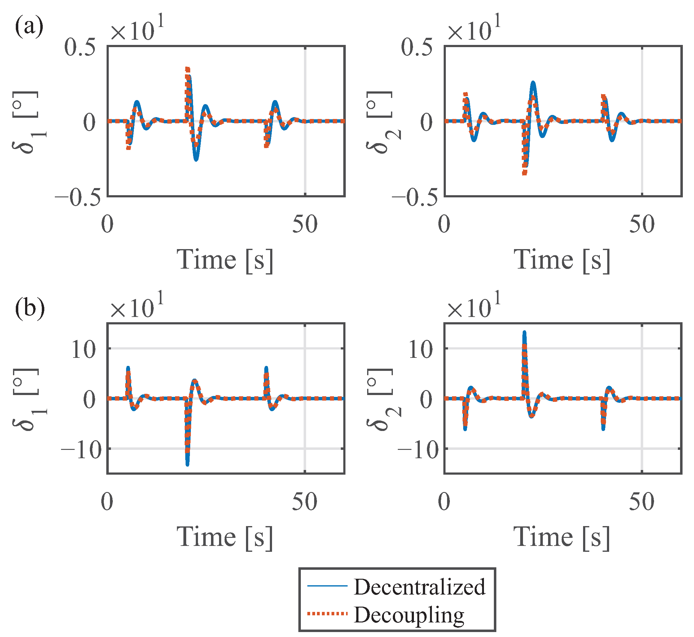
3.1. Simulation Results

In this section, the effectiveness of both control allocation approaches is tested through simulations using the control scheme shown in Figure 8, where the inverse propulsion system dynamics (i.e., $P_{inv}$) is obtained according to the control allocation schemes of the previous section.

A pair of PID controllers was designed for the pitch and yaw angles, $C_{\theta }$ and $C_{\psi }$, respectively, using Equation (21) as a design model. That is, it was assumed that the propulsion system is fully decoupled and compensated. This assumption yields a pair of simple double-integrator dynamics, which are controlled through direct pole placement and the specifications of

Table 2. Specifications.

Requirement	Pitch $\mathit{\theta }$	Yaw $\mathit{\psi }$
Overshoot $M_p$	<35%	<25%
Settling Time $T_s$	<11 s	<15 s

. These specifications aim at introducing a certain degree of bandwidth separation between the orientation angles and consider a slower response time for the propeller tilting servos than the propeller thrust. This aspect will become an important issue for the experimental implementation and is commented on later in the article. The resulting PID gains are reported in

Table 3. Simulation PID controller gains.

Constant	Pitch	Yaw
Proportional	2	1.5
Integral	0.1	0.1
Derivative	1.5	1

.

The simulations were performed with both control allocation approaches (i.e., decentralized and SVD-decoupled), the previously mentioned PID controllers and the non-linear model of the modified PVTOL test bench from Equation (19). In order to assess the resulting cross-coupling due to the input mixer algorithms, the following conditions were simulated:

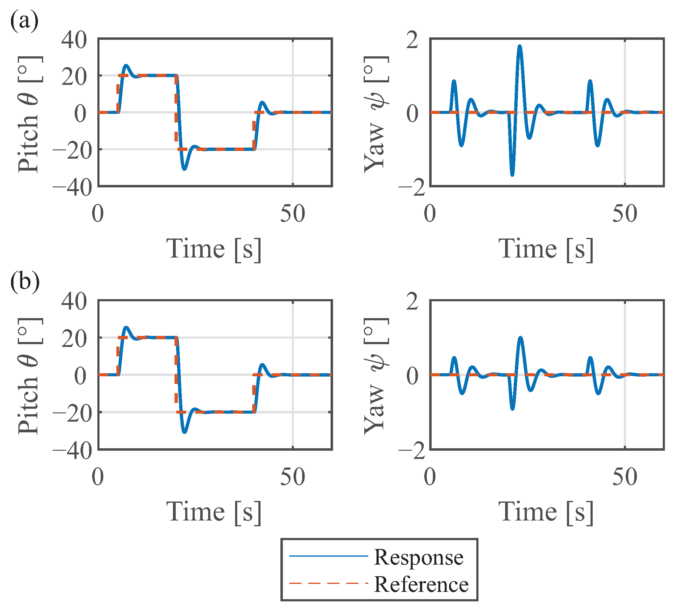
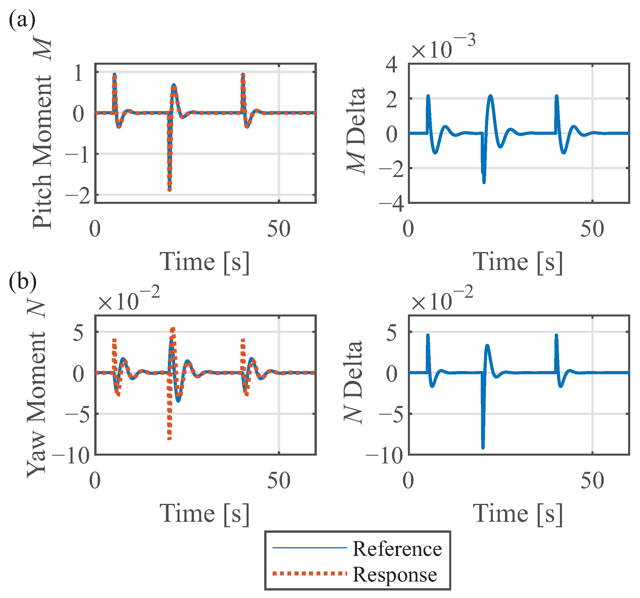
• Pitch-Varying Case: The pitch $\theta$ reference changes in steps, while the yaw $\psi$ reference remains constant at zero.
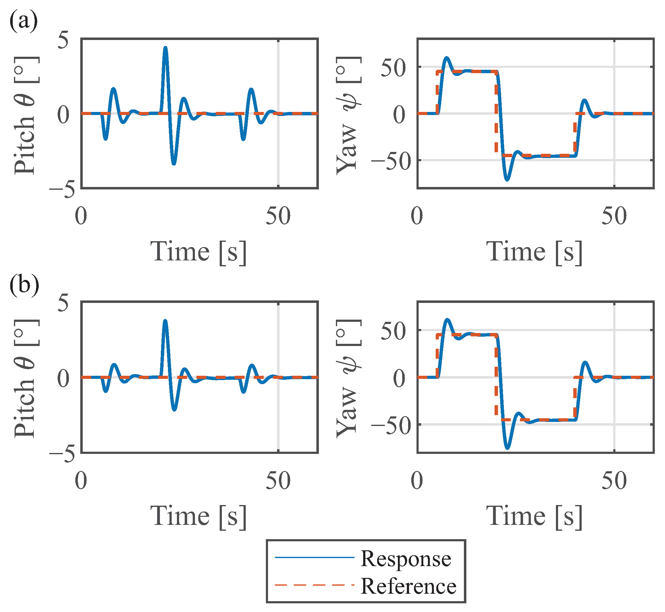
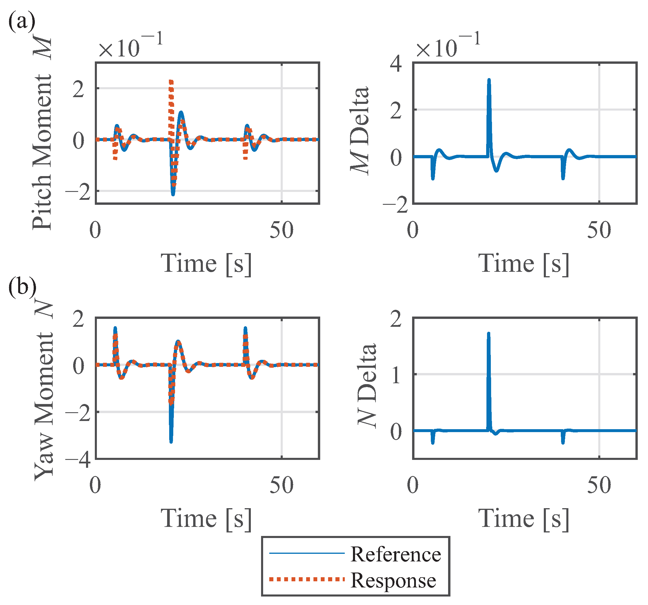
• Yaw-Varying Case: The yaw $\psi$ reference changes in steps, while the pitch $\theta$ reference remains constant at zero.

3.1.1. Pitch-Varying Case

Figure 9a shows the simulated responses of the pitch and yaw angles for the decentralized approach, while Figure 9b presents the same variables using the SVD-decoupling algorithm. This figure shows that while the pitch angle response of both approaches is similar and within the control specifications, the cross-coupling introduced in the yaw angle is significantly greater in the case of the decentralized input mixer.

In order to better assess the effectiveness of the SVD-decoupling control allocation approach, Figure 10 presents a comparison between the reference moments (i.e., $M,N$ and $M_{des},N_{des}$) and the actual moments exerted by the propulsion system for the simulation of Figure 9 with the SVD-decoupling approach. This figure shows that the resulting SVD-decoupling mixer has a very low error level (N and M deltas) and very good tracking capabilities. The greatest error level is observable in the case of the yawing moment at the time of the pitch angle step movement, which is when the propulsion system cross-coupling is at its highest.

3.1.2. Yaw-Varying Case

For the yaw variation simulations, Figure 11a shows the simulated responses of the pitch and yaw angles for the decentralized approach, while Figure 11b presents the same variables using the SVD-decoupling algorithm. Similarly to the pitch-varying case, the cross-coupling in the pitch angle due to variations in the yaw angle reference is reduced by using the SVD-decoupling mixer.

Finally, Figure 12 presents a comparison between the reference moments (i.e., $M,N$ and $M_{des},N_{des}$) and the actual moments exerted by the propulsion system for the simulation of Figure 11 with the SVD-decoupling approach. The greatest error level is observable in the case of the pitching moment at the time of the yaw angle step movement, which is when the propulsion system cross-coupling is at its highest.

3.1.3. Discussion

The previous results show that, in a simulated environment, the SVD-decoupling approach is effective in reducing the resulting cross-coupling, even when considering non-linear propulsion dynamics. In addition, the proper setting of the free variables when calculating the propulsion system inverse dynamics allowed obtaining similar responses to the physical insight approach. That is, the SVD-decoupling approach allows integrating physical insight easily. This is an important feature, because in most real applications, practical considerations have to be taken into account. For example, Figure 13 presents a comparison between the tilt-rotor angles for the simulations of the previous section considering both control allocation approaches. This figure shows that both approaches essentially produce the same overall tilt-rotor angles; however, the SVD-decoupling approach introduces slight adjustments, which resulted in a reduced cross-coupling.

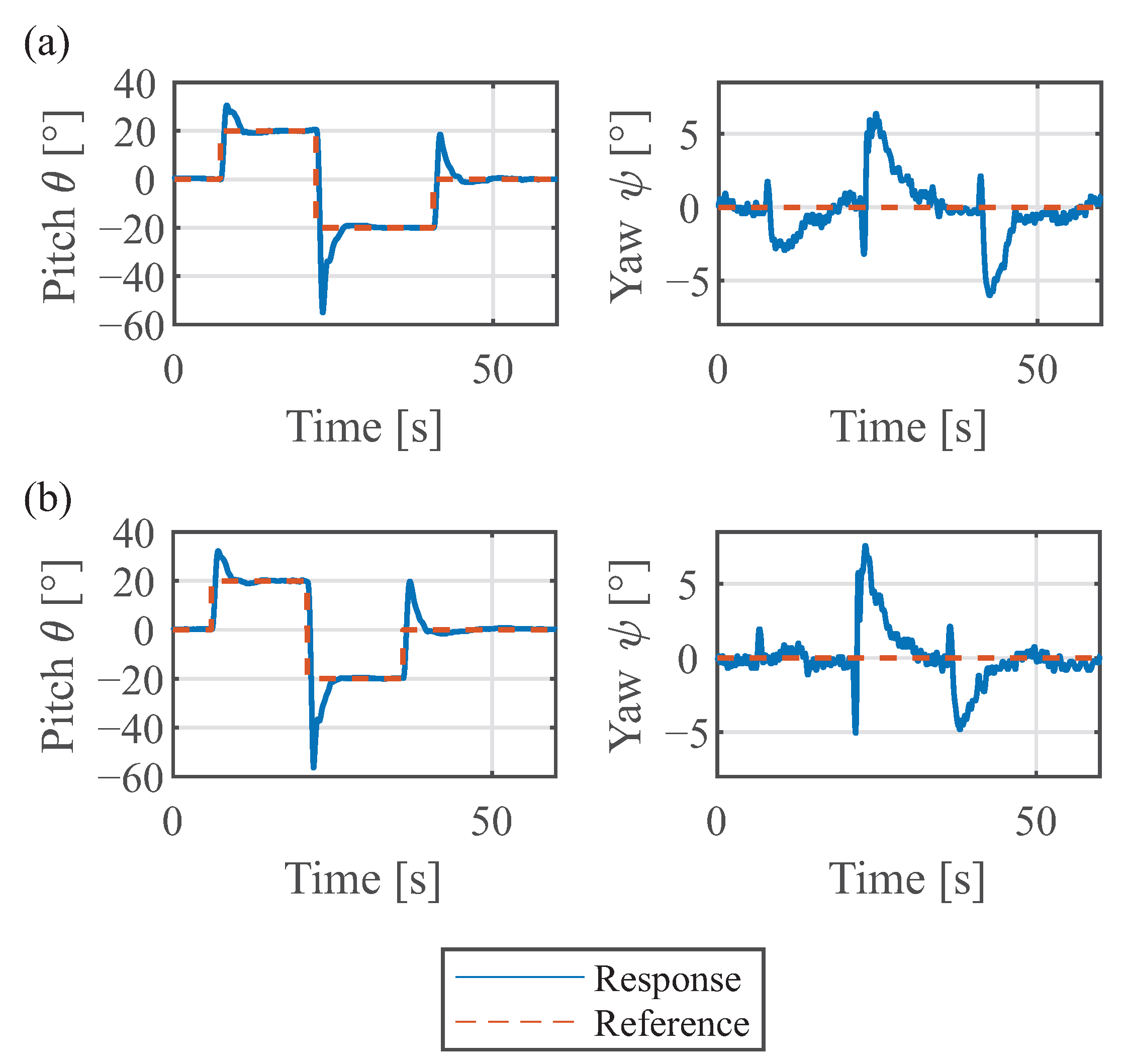
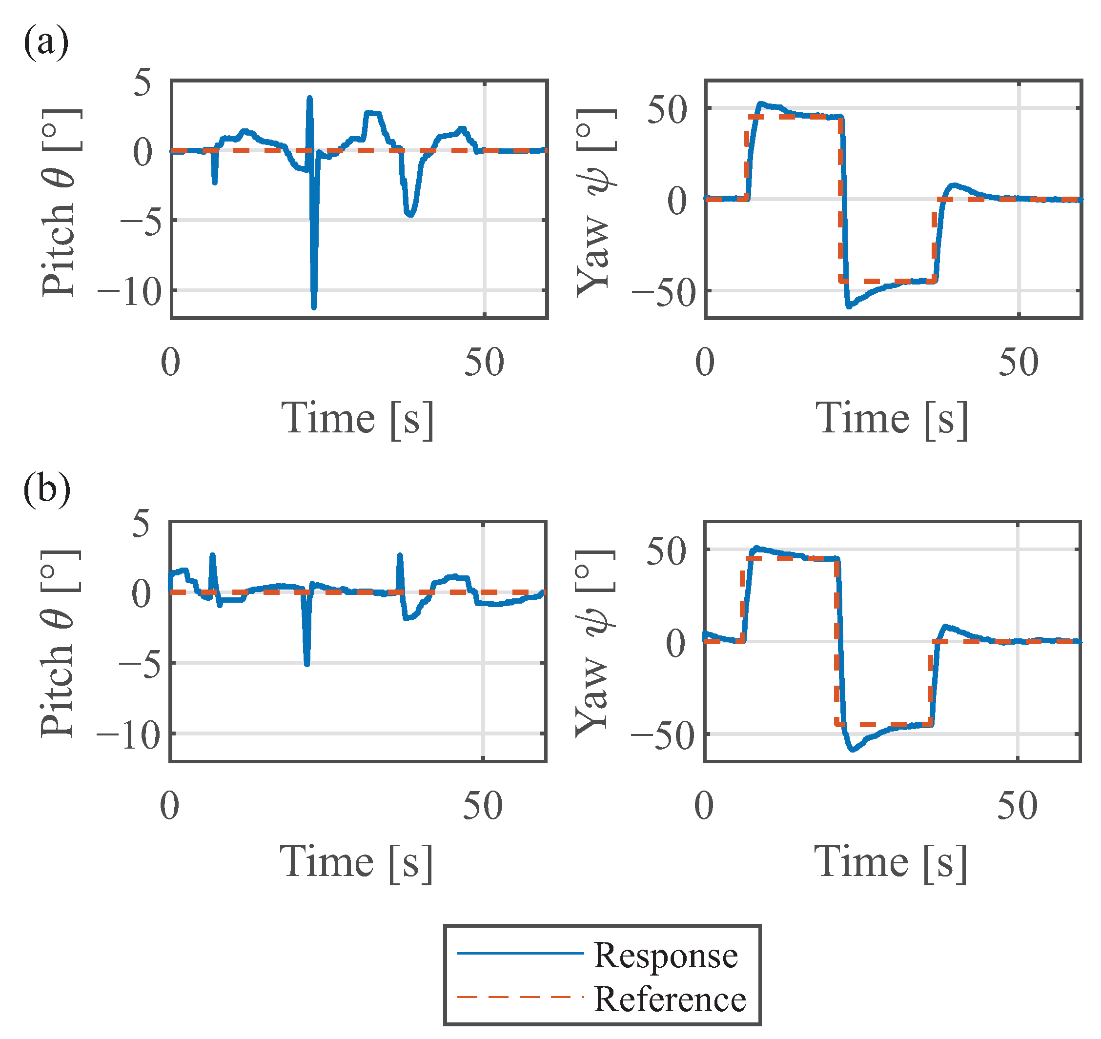
3.2. Experimental Results

The control system of Figure 8 was implemented experimentally using the test bench of Figure 3 and a similar set of experiments to those presented in the simulations was performed.

The PID gains of the previous section (i.e., simulation) were taken as a baseline in the tuning of the prototype’s controller. Since the simulated test bench equations (Equation (19)) did not account for friction damping, a slight adjustment of the PID gains was necessary to maintain the control specifications. A comparison of the frequency-domain response of the original (i.e., simulated) and the experimentally adjusted PID controllers is presented in Figure 14. This figure confirms that the main differences between these controllers are (1) decreased phase (damping) in the experiment and (2) increased gain for the experimental PID controller, which is in line with the effects of a higher level of friction in the experimental setup. The resulting PID gains used for the experiments are presented in

Table 4. Experimental PID controller gains.

Constant	Pitch	Yaw
Proportional	1.5	1.5
Integral	1	0.5
Derivative	0.5	1

. Both control allocation schemes were implemented using the same PID controllers.

3.2.1. Pitch-Varying Case

The experimental responses of the test bench when the pitch reference is modified for both control allocation approaches are shown in Figure 15. In comparison with the simulated responses from Figure 9, this figure shows that the pitch angle responses are more affected by the amplitude of the pitch angle variation in both approaches. For instance, the overshoot when moving the pitch angle reference from 20° to −20° is larger than in the simulated response. This could be mostly due to actuator saturation (absolute or rate) or other non-modelled dynamics. The effect is that the cross-coupling reduction in the yaw angle of the SVD-decoupling approach is reduced in the largest pitch reference modification (40° magnitude), but it is maintained in the other cases (20° magnitude). In addition, a greater reduction was observed for the positive pitch angle variation than the corresponding negative of the same magnitude. This suggests that there could be imbalances in the test bench, either mechanical or due to actuator mismatch.

3.2.2. Yaw-Varying Case

Figure 16 shows the experimental results when varying the yaw angle reference. In this case, the cross-coupling reduction in the pitch angle introduced by the SVD-decoupling approach is maintained in all cases, while the overall yaw angle response performance is similar for both approaches. The contrast with the pitch-varying case, where the cross-coupling was greater in the largest magnitude reference change, suggests an asymmetry in the response times of the main pitch and yaw actuators (i.e., electronic speed controllers for pitch and tilt servos for yaw in this case).

3.3. Quantitative Analysis

A quantitative summary of the experimental responses is presented in

Table 5. Mean Squared Error comparison between decentralized and decoupling controllers for pitch $\theta$ and yaw $\psi$ reference variations.

Experiment	DoF	Decentralized	Decoupling	$\mathsf{\Delta }$%
Pitch $\theta$	Pitch $\theta$	37.4525	38.2600	2.1560
Variation	Yaw $\psi$	4.1196	3.2768	−20.4583
Yaw $\psi$	Pitch $\theta$	2.3904	0.7042	−70.5405
Variation	Yaw $\psi$	118.6156	120.5088	1.5960

, which shows the Mean Squared Error (MSE) of the experimental responses of Figure 15 and Figure 16.

Comparing both control allocation approaches when varying the pitch angle reference, there was a reduction of $20.4\%$ in the MSE of the yaw angle cross-coupling when using the SVD-decoupling scheme. A reduction of $70.5\%$ in the MSE of the pitch angle cross-coupling was also observed when the yaw angle reference was modified with the SVD-decoupling scheme.

On the other hand, Table 5 also reveals that, interestingly, the cross-coupling reductions of the SVD-based scheme came at the cost of a slight increase in MSE at the reference angle responses. In particular, increases of $2.15\%$ and $1.59\%$ were observed for the pitch and yaw angles, respectively.

This trade-off of cross-coupling reduction and main angle tracking performance was not observed in the simulated responses, which suggests again that actuator limitations and asymmetry may be a possible explanation.

Figure 17 and Figure 18 present the error distribution of the experimental responses. A closer look at Figure 17, which corresponds to the experiment where the pitch angle reference is modified, shows that the error distribution for the yaw angle is considerably reduced with the SVD-decoupling approach, with much tighter quartiles overall, while the median is similarly close to zero in both cases. In contrast, for the pitch angle, the SVD-decoupling approach yields similarly large quartiles with a slightly larger range. In addition, the distribution of the inner quartiles with the SVD-decoupling approach is significantly skewed compared with the decentralized approach, while maintaining the same overall size, resulting in the median being farther from zero in the SVD-decoupling approach, which can explain the slight increase of MSE in this case.

In the case of the yaw varying experiment, Figure 18 shows that the error distribution of the pitch angle, which represents the cross-coupling in this experiment, is also considerably reduced with the SVD-decoupling approach, with all quartiles much closer to zero as well as the median. For the yaw angle, the SVD-decoupling approach yields a very similar error distribution to the decentralized approach, with the main differences being a median closer to zero and a slight skew to negative errors for the outer quartiles.

These figures confirm and extend the observations made with Table 5. That is, introducing the SVD-decoupling scheme reduces the cross coupling significantly while only slightly affecting the reference angle performance.

4. Discussion and Conclusions

In this article, a modified PVTOL configuration with an arbitrary number of co-linear tilting rotors was introduced as a baseline to study the control allocation problem found in many of the recently proposed VTOL aircraft designs. A general model for the resulting propulsion subsystem, as well as its linearization, was also developed. This linearization, which is necessary for many of the current control allocation strategies, is presented in a general and structured manner, to facilitate a better understanding of the effects of each of the physical parameters of the propulsion system.

Following the proposed modified PVTOL configuration, a two-tilting-rotor test bench was implemented experimentally. This test bench yields an over-actuated system which can be used to study the control allocation problem theoretically and experimentally. An SVD control allocation approach was developed for the resulting test bench. The proposed approach allows deriving an adequate input mixer algorithm for the over-actuated system, and it is shown that the remaining free degrees of freedom can be used to integrate physical insight and to solve general optimization goals (in this case, the minimization of error due to linearization).

The resulting SVD control allocation scheme is compared with a more traditional scheme derived by physical insight. It is shown that both approaches yield a similar use of the available control variables, with the SVD-based scheme introducing minor input modifications which allow obtaining a considerable decrease in cross-coupling in the test bench orientation angles.

Simulation and experimental results validate that the SVD control allocation scheme allows decreasing cross-coupling while maintaining the same overall performance as the traditional approach. The main deviations from the simulated and experimental results are due to the presence of friction damping in the experimental test bench, which was expected.

Interestingly, other smaller deviations suggest that actuator discrepancies can also have a significant effect on the resulting performance, that is, differences in actuator time responses, saturation levels, etc., due to the type of actuator, for instance, tilt-rotor servo dynamics vs. electric motor controller and propeller dynamics. Further research which incorporates better specific actuator properties is required to extend the benefits of decoupling control allocation schemes in general. This is an important finding, since many applications which require control allocation solutions use a mixture of dissimilar actuators.

Finally, the results support the continued use of the proposed modified PVTOL configuration, in either the presented two-rotor version or in a more complex configuration, for the study of the control allocation problem.

References

- EASA. MOC SC-VTOL, Proposed Means of Compliance with the Special Condition VTOL; Technical Report; European Union Aviation Safety Agency: Cologne, Germany, 2022. [Google Scholar]
- EASA. RMT.0731, Terms of Reference for Rulemaking Task, New Air Mobility; Technical Report; European Union Aviation Safety Agency: Cologne, Germany, 2021. [Google Scholar]
- Wang, X.; Cai, L. Mathematical modeling and control of a tilt-rotor aircraft. Aerosp. Sci. Technol. 2015, 47, 473–492. [Google Scholar] [CrossRef]
- Kong, Z.; Lu, Q. Mathematical Modeling and modal switching control of a novel tiltrotor UAV. J. Robot. 2018, 2018, 8641731. [Google Scholar] [CrossRef]
- Lu, K.; Liu, C.; Li, C.; Chen, R. Flight Dynamics Modeling and Dynamic Stability Analysis of tilt-rotor aircraft. Int. J. Aerosp. Eng. 2019, 2019, 5737212. [Google Scholar] [CrossRef]
- Sheng, H.; Zhang, C.; Xiang, Y. Mathematical Modeling and Stability Analysis of tiltrotor aircraft. Drones 2022, 6, 92. [Google Scholar] [CrossRef]
- Çakıcı, F.; Leblebicioğlu, M.K. Modeling and simulation of a small-sized tiltrotor UAV. J. Def. Model. Simul. Appl. Methodol. Technol. 2011, 9, 335–345. [Google Scholar] [CrossRef]
- Chen, C.; Shen, L.; Zhang, D.; Zhang, J. Mathematical Modeling and control of a tiltrotor UAV. In Proceedings of the 2016 IEEE International Conference on Information and Automation (ICIA), Ningbo, China, 1–3 August 2016. [Google Scholar] [CrossRef]
- Liu, Z.; He, Y.; Yang, L.; Han, J. Control techniques of Tilt Rotor Unmanned Aerial Vehicle Systems: A Review. Chin. J. Aeronaut. 2017, 30, 135–148. [Google Scholar] [CrossRef]
- Hegde, N.T.; George, V.; Nayak, C.G.; Kumar, K. Design, dynamic modelling and control of tilt-rotor uavs: A Review. Int. J. Intell. Unmanned Syst. 2019, 8, 143–161. [Google Scholar] [CrossRef]
- Bacchini, A.; Cestino, E. Electric VTOL Configurations Comparison. Aerospace 2019, 6, 26. [Google Scholar] [CrossRef]
- Amezquita-Brooks, L.; Liceaga-Castro, E.; Gonzalez-Sanchez, M.; Garcia-Salazar, O.; Martinez-Vazquez, D. Towards a standard design model for quad-rotors: A review of current models, their accuracy and a novel simplified model. Prog. Aerosp. Sci. 2017, 95, 1–23. [Google Scholar] [CrossRef]
- Amezquita-Brooks, L.; Hernandez-Alcantara, D.; Santana-Delgado, C.; Covarrubias-Fabela, R.; Garcia-Salazar, O.; Ramirez-Mendoza, A.M.E. Improved Model for Micro-UAV Propulsion Systems: Characterization and Applications. IEEE Trans. Aerosp. Electron. Syst. 2020, 56, 2174–2197. [Google Scholar] [CrossRef]
- Grau, S.; Kapitola, S.; Weiss, S.; Noack, D. Control of an over-actuated spacecraft using a combination of a fluid actuator and reaction wheels. Acta Astronaut. 2021, 178, 870–880. [Google Scholar] [CrossRef]
- Qin, Z.; Liu, K.; Zhao, X. A smooth control allocation method for a distributed electric propulsion VTOL aircraft test platform. IET Control Theory Appl. 2023, 17, 925–942. [Google Scholar] [CrossRef]
- Santos, M.; Honório, L.; Moreira, A.; Garcia, P.; Silva, M.; Vidal, V. Analysis of a Fast Control Allocation approach for nonlinear over-actuated systems. ISA Trans. 2022, 126, 545–561. [Google Scholar] [CrossRef] [PubMed]
- Hamandi, M.; Usai, F.; Sablé, Q.; Staub, N.; Tognon, M.; Franchi, A. Design of multirotor aerial vehicles: A taxonomy based on input allocation. Int. J. Robot. Res. 2021, 40, 027836492110259. [Google Scholar] [CrossRef]
- Zheng, X.; Yang, X. Improved adaptive NN backstepping control design for a perturbed PVTOL aircraft. Neurocomputing 2020, 410, 51–60. [Google Scholar] [CrossRef]
- Bonilla, M.; Blas, L.; Azhmyakov, V.; Malabre, M.; Salazar, S. Robust structural feedback linearization based on the nonlinearities rejection. J. Frankl. Inst. 2020, 357, 2232–2262. [Google Scholar] [CrossRef]
- Łakomy, K.; Madonski, R. Cascade extended state observer for active disturbance rejection control applications under measurement noise. ISA Trans. 2021, 109, 1–10. [Google Scholar] [CrossRef] [PubMed]
- Offermann, A.; Castillo, P.; Miras, J.D. Control of a PVTOL with tilting rotors. In Proceedings of the 2019 International Conference on Unmanned Aircraft Systems (ICUAS), Atlanta, GA, USA, 11–14 June 2019. [Google Scholar] [CrossRef]
- Harindranath, A.; Arora, M. A Systematic Review of User-Conducted Calibration Methods for MEMS-based IMUs. Measurement 2023, 114001. [Google Scholar] [CrossRef]
- Otegui, J.; Bahillo, A.; Lopetegi, I.; Díez, L.E. Performance Evaluation of Different Grade IMUs for Diagnosis Applications in Land Vehicular Multi-Sensor Architectures. IEEE Sens. J. 2021, 21, 2658–2668. [Google Scholar] [CrossRef]
- de Alteriis, G.; Conte, C.; Lo Moriello, R.S.; Accardo, D. Use of Consumer-Grade MEMS Inertial Sensors for Accurate Attitude Determination of Drones. In Proceedings of the 2020 IEEE 7th International Workshop on Metrology for AeroSpace (MetroAeroSpace), Pisa, Italy, 22–24 June 2020; pp. 534–538. [Google Scholar] [CrossRef]
- Villarreal Valderrama, J.F.; Takano, L.; Liceaga-Castro, E.; Hernandez-Alcantara, D.; Zambrano-Robledo, P.D.C.; Amezquita-Brooks, L. An integral approach for aircraft pitch control and instrumentation in a wind-tunnel. Aircr. Eng. Aerosp. Technol. 2020, 92, 1111–1123. [Google Scholar] [CrossRef]