1. Introduction
Multirotor systems in the present day have drawn major attention owing to their versatility in carrying out various applications [
1]. Their ability to transport payloads from point to point opens their usage in many different fields, including agriculture, military, postage, and media. However, carriage of suspended payloads poses a challenge to multirotor operation as the system’s dynamics are altered by the extra mass and swinging motion of the payload. The addition of a suspended payload adds an extra 2 Degrees of Freedom (DoF) to the existing 6 DoF multirotor UAV system. A multirotor-slung load system has different characteristics to that of a conventional multirotor, with the addition of a mass moment of inertia and the dynamics of the payload it carries. To this degree, the effects of payload mass, size, and distribution on the system’s stability and control have previously been analyzed by researchers. Additional stability and control issues are introduced by the payload’s swinging motion as they tend to cause disruptions and instability. Keeping the payload stable and maneuverable while maintaining the UAV’s location and orientation poses a challenge in terms of control.
There have been several control strategies proposed to tackle this interesting problem. In Ref. [
2], an Adaptive Linear Quadratic Regulator with input shaping is proposed, with an output weighing variation, where the work seeks to track desired trajectory of a quadcopter together with reducing the swing of the payload it carries. Hanafy et al. create a new genetic-based Fuzzy Logic Controller to reduce the oscillations caused by a quadrotor-suspended load in Ref. [
3]. They use a genetic algorithm, attempting to optimize membership function distributions of the control inputs and outputs. In Ref. [
4], a cable-suspended weight is tracked using the Lyapunov theory aided by backstepping methods to obtain a specific trajectory described using a time-parameterized position vector. The dynamics of both the quadrotor-slung load and cable direction, in addition to the coupling that they possess with the quadcopter, are taken as one single part of the nonlinear backstepping controller design. By developing a fractional order sliding mode control, El Ferik et al. [
5] intend to propose a new method of controlling a quadrotor-slung load system, in addition to the swing angle of an imposed suspended load. A robust tracking control problem dealing with a quadrotor subject to system nonlinearities, coupling of inputs, aerodynamic irregularities, and external factors, such as wind, is analyzed through quantitative simulation studies in Ref. [
6], focusing on position and attitude control. With tracking control and disturbance elimination of multirotor-slung load systems, Liu et al. [
7] examine an adaptive hierarchical sliding mode controller, employing a sliding mode disturbance observer operating such that it converges in a fixed time interval. To address the issue of underactuated features, the projection operator is used to build the adaptive law, and the hierarchical sliding mode control concept is employed to establish the controller. In Ref. [
8], a quadrotor subjected to disturbances is controlled by an integral non-singular hyperplane SMC scheme, which also assures precise tracking when these disturbances are present. With the consideration that wind gusts make the tracking operation of a drone more difficult, in order to complete tracking tasks when wind gusts emerge, a Proportional-Integral-Derivative (PID) control, which can tune itself to adjust to these changes, is derived in Ref. [
9]. A supervisory control created with the Lyapunov method is introduced to display the stability of this approach when taking bounded disturbances into account. Cui et al. propose a Linear Active Disturbance Rejection Control, coupled with an input shaper, to create an attitude controller in Ref. [
10]. In Ref. [
11], the robust H control methodology known as linear matrix inequality (LMI), which is widely used, is chosen for the linear controller design. In addition, an observer is introduced for estimating load angles. Previous control strategies include Linear Quadratic Regulator (LQR) [
12], fault tolerant flight control [
13], geometric control [
14], nonlinear model predictive control [
15], and neural networks [
16].
In recent years, multi-surface sliding mode control (MSSC) has become a promising control method. Aiming to improve robustness and tracking precision in dynamic systems, it tackles the constraints of standard sliding mode control (SMC) by introducing numerous sliding surfaces. In traditional sliding mode control, the system’s states are guided down a desired trajectory by a single sliding surface. It can be subject to uncertainties, disturbances, and nonlinearities, which can result in performance degradation even though it can be beneficial in some situations. By separating the control space into numerous sliding surfaces, MSSC overcomes these difficulties. Various applications of MSSC, such as those in robotics, aerospace, automotive, and power systems, have been studied by researchers. For example, in robotics, where precise trajectory tracking is essential, MSSC has been used to operate manipulator arms and mobile robots. To manage uncertainties related to atmospheric conditions and outside disturbances, it has also been used in flight systems. MSSC offers improved robustness to uncertainty, where the control system can adjust to various operating situations by using several sliding surfaces, effectively reducing the effect of uncertainties on system performance. Additionally, it provides better tracking precision, as multiple sliding surfaces enable more accurate control and improved tracking of desired trajectories by allowing the control action to be tuned to areas of the control space. It has been used across different fields as an effective control method. A class of single-input, single-output (SISO) systems was the primary target for the development of multi-surface sliding control (MSSC). In this study, the MSSC is extended from SISO systems, such that it addresses a specific kind of Multi-Input Multi-Output (MIMO) system. In addition, the underactuated systems, which are analyzed in this work, may be altered into high-order MIMO nonlinear systems with mismatched uncertainties by changing the co-ordinate, as the MSSC is resilient against unknown disturbances. Then, this UAV control problem can be directly solved using the MSSC algorithm. Additionally, MSSC designs for UAV systems with suspended payloads are still in the early stages. Many control methods for such systems are created by decoupling the longitudinal and lateral dynamics separately due to the coupling effect of UAV dynamics [
17]. Our approach provides a comprehensive control methodology by cascading the translational and rotational systems in addition to addressing the underactuated concerns. A reliable and desired control methodology for SISO systems has been demonstrated using MSSC [
18] and high-order sliding mode control [
19] for the regulation of underactuated nonlinear systems subjected to mismatched uncertainties, as in Refs. [
20,
21]. Numerous desirable characteristics of adaptive MSSC, including its resistance to both matched and mismatched uncertainties of several types, such as parametric variations and external disturbances, as well as the system’s convergence to zero error, are useful for flight dynamic control. With this being considered, MSSC has been used in different applications as an effective control method. Ref. [
22] addresses the issue of chained stabilization of a class of nonholonomic systems with known and unknown disturbances. The suggested design strategy is based on an adaptive MSSC applied to a discontinuous transformation of the perturbed nonholonomic system. In Ref. [
23], a Takagi–Sugeno fuzzy model (TSFM)-based multi-objective resilient control scheme is proposed for a set of indeterminate nonlinear systems, which is then applied to a two-link robot system containing both matched and mismatched uncertainties. Hamood et al. track and control the height and angles of a 3-Degree-of-Freedom helicopter using a control strategy derived from the MSSC. In Ref. [
24], Alqumsan et al. analyze the operation of continuum robots while taking mismatched uncertainties into account and propose a control strategy. Cosserat rod theory is used to construct the dynamic model of the system to develop the controller, and multi-surface sliding mode control is used to ensure robustness of the system against mismatched uncertainties. In Ref. [
25], a multiple-surface sliding mode control based on disturbance observers is developed. It estimates the uncertainties as well as the derivatives of the virtual inputs.
Finite-time control is essential for control systems in terms of quick response to real-world situations, optimization of transient response, reduction in energy consumption, and efficacy of safety and performance. Previous finite-time control approaches have been proposed, such as a super-twisting algorithm [
26], a nonlinear cascade structure [
27], geometric control [
28], and trajectory tracking control [
29]. Taking these factors into consideration, this paper will propose both a robust and an adaptive finite-time multi-surface sliding mode control. The main contribution of this paper lies in the derivation and subsequent application of a finite-time multi-surface sliding mode control to a multirotor-slung load system. Unlike most existing studies, which consider planar (2D) dynamics for a pendulum, the slung load is modeled using the spatial (3D) dynamics of a single pendulum. While the dynamic model of the single pendulum slung load itself is defined, its effect upon the behavior of multirotor UAVs is unknown and hence, can be used to represent other such disturbances to the normal behavior of the UAV. These disturbances may arise due to external factors, such as wind and obstacles, or internal factors such as parametric changes occurring due to additions to the drone’s structure, including the addition of a suspended payload itself.
The rest of this paper is outlined as follows. First, the dynamics of a multirotor will be derived, together with those of a single pendulum, representing a slung load to be transported by the multirotor. The dynamics of these two systems will cascade to form a single system (
Section 2.1 and
Section 2.2). A multi-surface sliding mode control strategy will then be proposed and its stability verified in
Section 2.3. An adaptive version of the same controller will then be derived in
Section 2.4. In
Section 3, both these controllers will individually be applied to the multirotor-slung load system for the stabilization of the multirotor on its travel path, along with the suppression of the slung load oscillations that take place. Their performance in different scenarios and with imposition of external disturbances will be presented. An analysis of the results obtained from these simulations will be analyzed in
Section 4.
Section 5 provides some conclusions.
2. Methodology
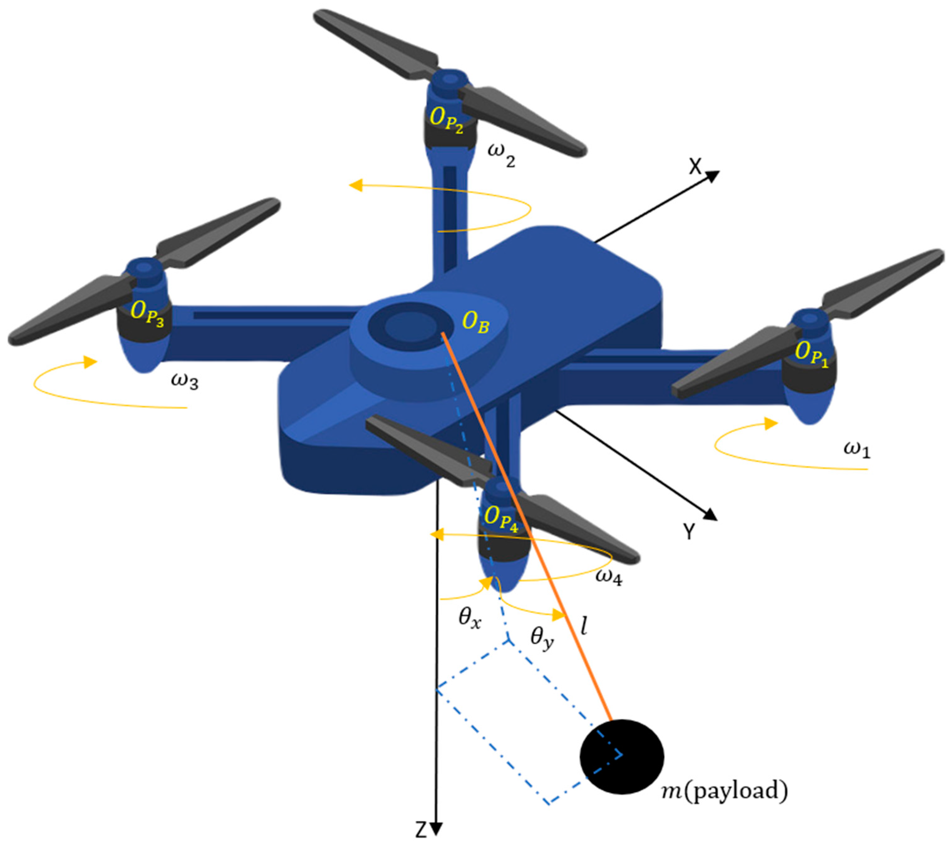
In this section, we define the dynamics of a multirotor and its suspended payload, which are then cascaded together to form a single system. This is the system upon which the proposed controllers will be applied and subsequently compared. The characteristics of the multirotor slung load system are as shown in
Figure 1. Let
and
denote the translational and rotational state vectors of the system, such that
represents the overall system state vector, with
, and
denoting the multirotor position along their respective co-ordinate axes,
, and
representing the roll, pitch, and yaw about each respective co-ordinate axis, and
and
being the payload tilt angle about the
x-axis and
y-axis, respectively. We take the mass of the multirotor to be
and the payload it is carrying to have a mass
2.1. Multirotor Dynamics
We consider a multirotor, specifically a quadrotor with 4 rotors, with the dynamics defined in our previous work [
30].
represents the rotation of a frame 2 into a frame 1.
These are the standard rotational matrices of the frame in terms of its roll, pitch, and yaw, where shorthand notation is used to complete the rotational matrix, such that
and
.
where
where i = 1…, n (for this quadrotor, n = 4), and L is the multirotor arm’s length, measured from the body frame center (
to the center of a propeller (
). The torque acting on any propeller
, denoted as
, is first obtained using Euler’s angular momentum theory:
where
represents each propeller’s inertia matrix,
denotes vector
’s
z-axis component,
, the modulus of elasticity between
and the counter-rotating torque about
axis,
and
the angular velocity of the
propeller. If
is the
propeller’s produced thrust, we obtain
where
is a fixed proportionality constant. Applying the fundamental theorem of mechanics for the body frame, together with Euler’s angular momentum theory, we obtain
where
is the inertial matrix governing the multirotor body, and
represents force due to drag.
Considering an n-propeller multi-copter, where
and
and using the above equations, we acquire
2.2. Slung Load Dynamics
In this section, the slung load dynamic model is derived using Lagrange’s modeling approach, in which we take the suspended payload to be a simple pendulum. When the payload is considered a point mass (
), the kinetic energy is only translated. The spatial angle of the cable can be used to determine the precise location of the payload by ignoring cable hoisting and keeping the cable length fixed at
. The pendulum displacements are characterized by
and
, which denote the rotation of the payload about the inertial x- and y-axes, respectively. A linear damping term is used to mimic the physical dampening of the pendulum swing. Using Kane’s equation, the dynamical model is given by
where
represents the mass–inertia matrix,
denotes the Coriolis force matrix,
represents a vector containing the forces of gravity acting upon the system, and
is a Jacobian matrix for the system input vector
. The payload orientation and position along the co-ordinate axes are first defined, aiding in deriving the Lagrangian model of the system. For this, we take the payload co-ordinates to be
Differentiating (12) with respect to time and accounting for angular velocity, we obtain
which gives us the velocity vectors of the hook.
Differentiating (13) and accounting for the angular acceleration, we have
Now, according to Lagrange’s modeling equation,
Here, two independent variables, and , are considered as the generalized co-ordinates, collectively taken as . The associated hook-and-payload pendulum system is controlled by the input variables collected from the drone position variables x, y, and z.
The difference between the system’s potential and kinetic energies yields the Lagrangian, i.e.,
The potential energy,
, is obtained as
The kinetic energy,
, is then found using
Substituting (12) into (17) and (13) into (18) provides results for the potential and kinetic energies. Substituting these results into (16) provides the Lagrangian
, which is then substituted into (15) to provide the equations governing the slung load pendulum:
We rearrange (11), such that the acceleration, and subsequently the velocity and position of the system, can be obtained—giving us an idea of the quadrotor’s behavior—which can be performed as follows:
where
represents the desired position of the system. The coefficients of
in (19)–(23) define the contents of matrix
. Similarly, the coefficients of
yield the contents of matrix
, and the vector
comprises vectors dependent on gravitational acceleration
. The pendulum dynamics cascade with the quadrotor’s linear dynamics, represented as
.
Defining
,
and rearranging subsystems
and
yield
where
where the external disturbances affecting the system’s rate of change in angular and linear momenta are denoted by
and
, respectively.
and , respectively, denote the system’s linear and angular co-ordinates in the body frame.
Differentiating
with respect to time, we acquire
where
It is understood that and can be defined like , while and can be defined like .
We can rewrite (32) as
where
These represent the Jacobian matrices, which multiply the control law, , of the multirotor. This control law is defined for the two controllers in the next two sections.
2.3. Finite-Time MSSC
In this section, a robust finite-time multi-surface sliding mode control is presented. This is applicable to Multi-Input Multi-Output (MIMO) systems. First, we show that the sliding surfaces of the controller can achieve stability in a finite time. For this, we use the Lyapunov stability theory.
Let us consider a nonlinear system which is time-invariant, where . This system is said to be globally asymptotically stable if for every trajectory for the system, we have as , where is known as the system equilibrium point, such that . Furthermore, considering a function , the function is said to be positive definite if
- (i)
- (ii)
- (iii)
as
Hence, if we consider a function such that V is positive definite and , with , then the system is said to be globally asymptotically stable, i.e., all trajectories converge to zero as .
With this in consideration, let us take a system
, nonlinear and continuous in nature, such that f(0) = 0. If there exists a Lyapunov function
and real numbers
and
where
then we can say that the start of the nonlinear system is universally fast finite-time stable, and its settling time is given by
Alternatively, a control Lyapunov function (CLF), satisfying , which is nonlinear and dynamic in nature, may also guarantee universal finite-time convergence of the system, where the settling time is given by However, comparing the nonlinear CLF previously defined with linear dynamic equation , the latter provides a slower converging time when its initial condition is distant from zero. However, the finite-time convergence is understood by its growth rate, which is exponential in nature, as , since as for , . As a result, converges faster than for large , albeit the linear CLF closed-loop system-based asymptotic stability.
One quick resolution to this issue is to consider a CLF in agreement with (39). Looking at settling times and , if , we find since .
From this, we can say the closed-loop system with CLF, in agreement with (39), is a fast finite-time stable system. For
, let
, where
and
are positive odd integers, such that
. Some sliding variables
are first presented as
where
denotes a virtual controller.
represents the information of each variable describing the system, in this case its position, velocity, and acceleration, depending on the value of
. Therefore, it may be utilized to design a sliding variable and subsequently a controller. The proposed sliding variable (41) is utilized for a set of high-order nonlinear systems.
In (46), the virtual controller is designed in the form
where
If the multi-surface variables,
, this results in
, subsequently implying that
.
To further analyze the control, a few lemmas are explained below:
Lemma 1. The following Minkowski’s inequality [
31]
holds good for all real numbers zi, where i = 1,…,n, and 0 < k ≤ 1: Lemma 2. For some positive real numbers and some real-valued functions , > 0, the following holds true, according to [
32]:
The necessary sliding mode control laws may now be developed, attempting to ensure the convergence of the sliding surfaces in n steps.
We take the first sliding variable
Choosing the Lyapunov function
, we acquire
Let us consider a virtual control law
, defined as
with
,
, and
. Using the inequality
, we obtain
At step k − 1, where
, let as assume that the
virtual control is given by
such that
satisfies
where
is some known positive smooth function. Using induction, it can be shown that
Taking k = k + 1 to obtain the (k + 1)th virtual controller in (48), with
yields
For the final step, using the inductive argument carried out so far, we can show that
Theorem 1. For the sliding variable , taking the virtual control, as defined in (46) and (48), and the final control aswhere
and
, and is some known smooth positive function, the sliding variables are found to converge to the sliding surfaces in a fast finite time , where with denoting the Lyapunov candidate function’s initial value in (57). Proof. We see that if
, then
If
if the design process in the above Equations (46)–(55) is carried out, using the property
, the following Lyapunov function may be utilized:
We can show that the final controller in (55), with
, results in
From (58) and the Lyapunov function, as defined in (52) and (57), where with , results in , while with the definition of in (45), it can be concluded that all sliding variables converge at the sliding surfaces in a fast finite time .
From (48) to (58), it is seen that the sliding variables where can converge at the sliding surfaces in time . □
2.4. Adaptive Fast Finite-Time MSSC
In this section, an adaptive version of the controller defined in
Section 2.3 will be proposed. Initially, some assumptions are made in investigating the control:
- (i)
For , some undefined functions exist, such that .
- (ii)
A known continuous function exists, where , and .
We consider the same sliding variables as in (41), but for the subsystem such that . Considering that is unknown, an adaptive virtual control law is designed to ensure the system’s finite-time stability.
Lemma 3. Taking assumption (i) into consideration, if the subsystem defined above has and a virtual controller is selected aswhere , with adaptive parameter updated as Then —the initial condition of the system:
Case 1: if
, the state vector
will arrive at zero in a finite time
, such that
Case 2: if
,
will arrive at zero in a finite time
, such that
where
represents the Lyapunov function candidate such that
and
.
To verify the convergence of to zero within time , we will show that .
Let
be some new unknown parameter,
be its estimate, and
. Differentiating
with respect to time, we obtain
Combining (59),(60), and (63), for
, we arrive at
Case 2(a): For , since By (61), arrives at zero in finite time.
Case 2(b): For
as
and considering
. The time taken,
, for
to reach zero can be obtained as
which is like case 2 (62). After reaching time
the system state
takes a finite time
to converge to zero. Thus, with these conditions,
arrives at zero in finite time
.
For step
, when
similar steps are followed for the subsequent process as in step 1. For the subsystems,
For stability of the system within the pre-determined finite time, along with the existence of the adaptive control laws, the following requirements must be satisfied:
Under Assumption (i), consider
subsystems (68), such that
. If
and some Lyapunov functions
and
exist, and a set of virtual controllers
given by
such that
are continuous functions and
where
then for
—the initial condition for each system state:
Case 3: if
,
will arrive at zero in finite time
where
, with representing the peak of the unmatched functions.
Case 4: if , similar to case 2(a), arrives at zero within finite time , such that , with .
Step n: Considering the principle of mathematical induction as in [
33], it is understood that
where
represents the Lyapunov function candidate that we consider, such that
.
From (72), we can now verify that the overall system controller is defined by
with updating law
where
results in
From (75), it is understood that every path of the closed-loop system from (68) to (74) universally provides finite-time stability when taking Lyapunov stability criteria into consideration.
Theorem 2. For a set of unmatched nonlinear systems, if the control laws are designed as in (59), (69), and (73), respectively, where , , and are taken in accordance that the inequalities below are satisfied:then the state will arrive at zero in finite time where the true control signal is bounded. Proof. Considering a continuous, nonlinear system
, let there be a
Lyapunov function and some real numbers
, where
is positive definite and
Then, the origins of the system
are universally fast finite-time stable and the settling time, dependent on
(the initial state), can be obtained using
The inequalities in (77) and (78) ensure faster finite-time stability. From this, we see that the sliding surfaces converge in sequence within finite time T. We obtain , then . Similarly, . The point of equivalence, , is arrived at. From (71), as (76) holds good and , then the virtual controllers stay bounded, from which it is deduced the actual control signal also remains bounded. □
3. Results
To verify the effectiveness of the proposed controllers, each control is applied to the quadrotor-slung load system whose dynamics are defined in this work. While applying the robust and variable controllers to the system model derived in
Section 2.1 and
Section 2.2, the following vectors are considered for the dynamics of the overall system.
The parameters defining the multirotor and the slung load are displayed in
Table 1. In each case, the initial flight condition is taken as (x, y, z) = (0, 0, 0) and
. The desired trajectory is varied according to the simulation being implemented. The controller parameters are selected as
; a diagonal matrix of order
,
and
where
and
are also matrices of the same order as
.
, where represents the position of the multirotor, denotes the position of the slung load as defined in (12), and represents the orientation of the multirotor. Furthermore, , with calculated as defined in (13), and and representing the linear and angular velocities of the multirotor, respectively. Finally, , with calculated as in (14), and denoting the respective linear and angular accelerations of the system.
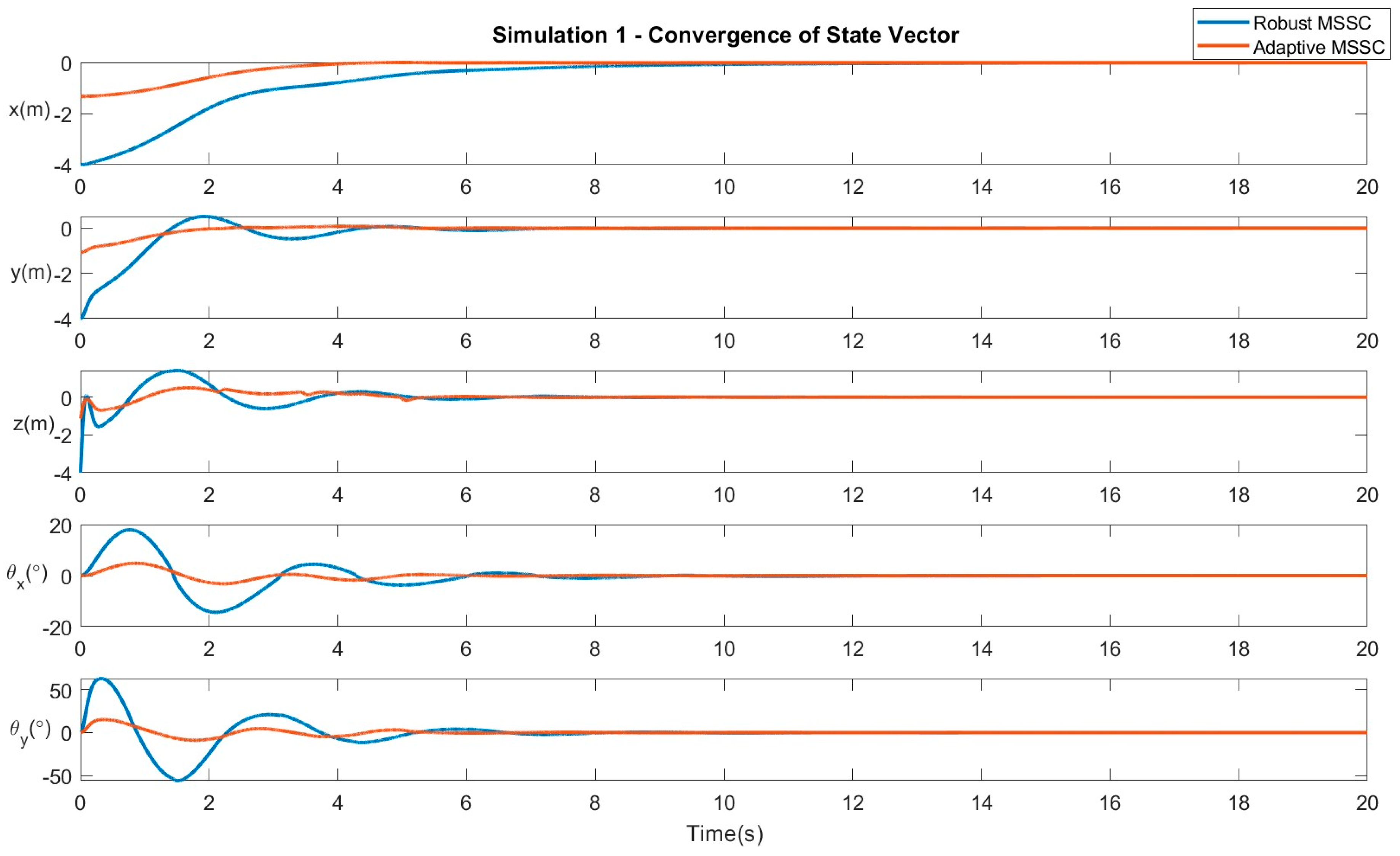
Four different MATLAB simulations are implemented to display the behavior of the quadrotor-slung load system upon application of the robust and adaptive MSSC in all planes. The aim is to suppress the oscillations of the pendulum slung load (, while simultaneously ensuring the arrival of the multirotor at its desired locations, in addition to the suppression of any external disturbances within a finite time (<2 s). The error in the position of the multirotor and the oscillation of the slung load pendulum about the co-ordinate axes should tend to zero within a finite-time interval.
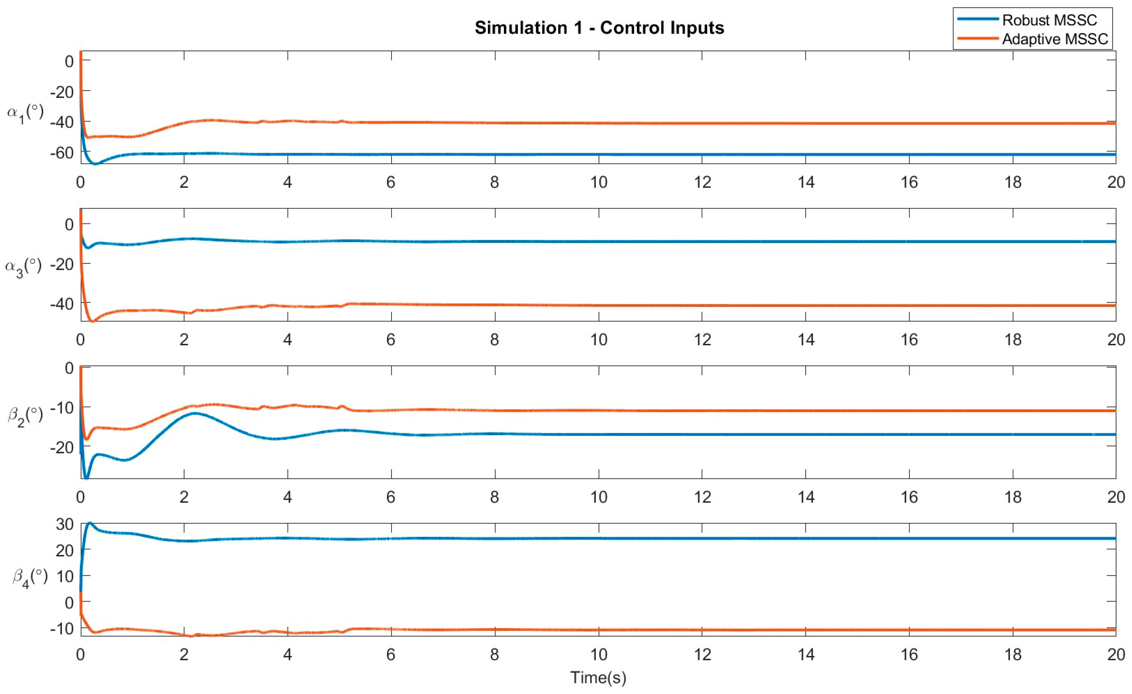
Simulation 1 − Linear movement: The system follows a path from the origin (0,0,0) to a point (3,2,1) in space. Hence,
.
Figure 2 verifies the convergence of the system states, i.e., the quadrotor position and the payload swing angle, to the desired position.
Figure 3 displays the control efforts necessary for the robust and adaptive variants of the proposed controller.
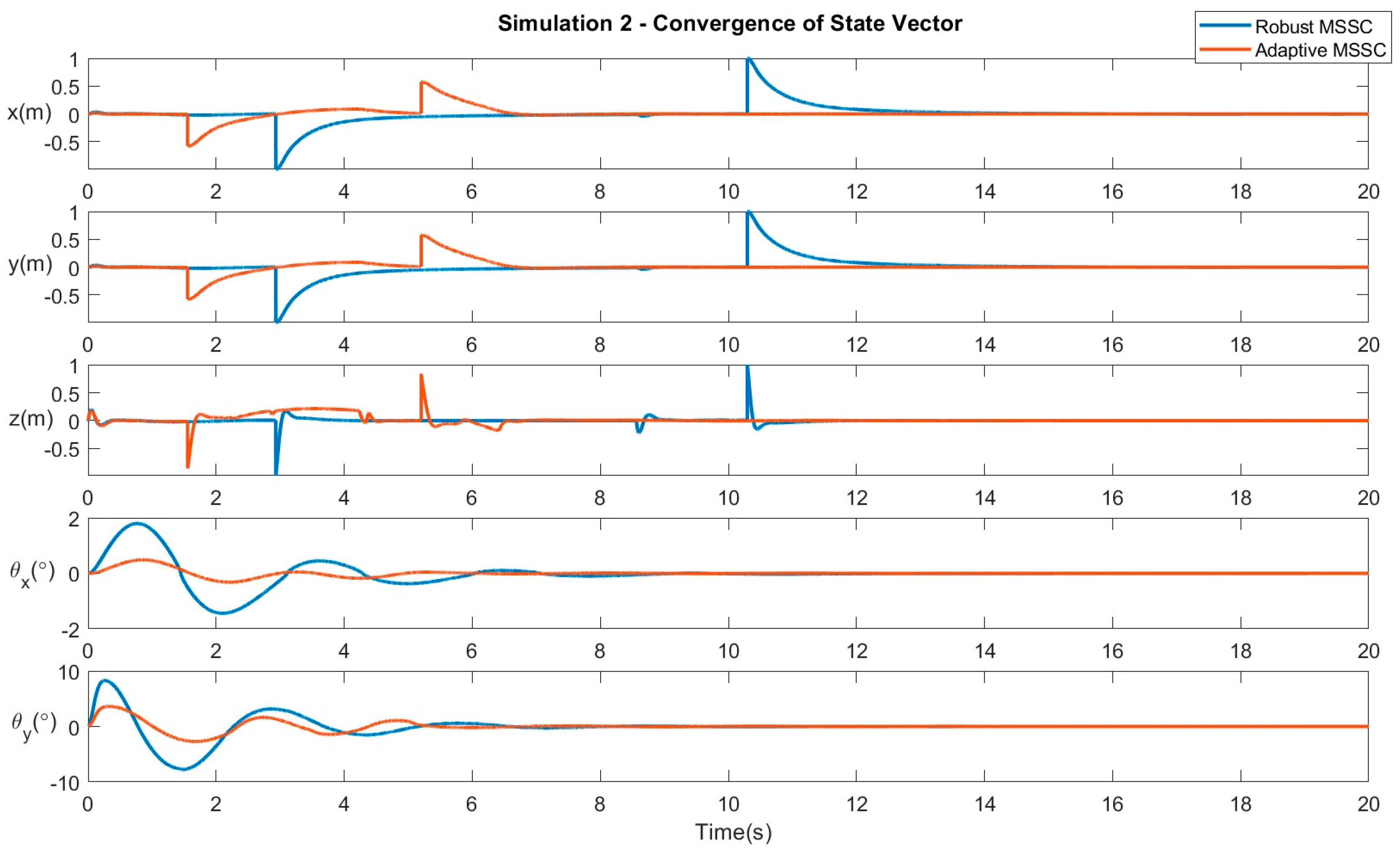
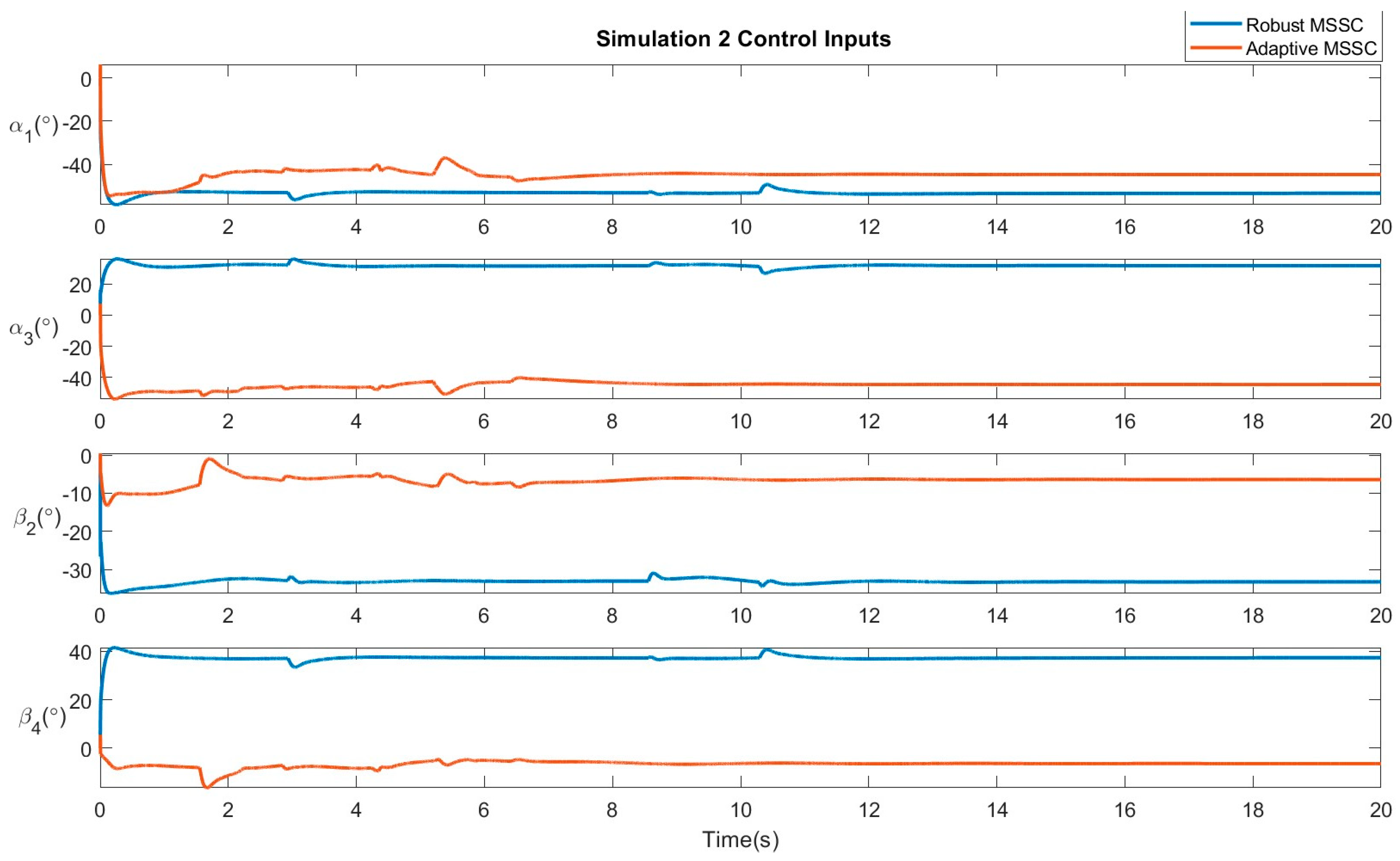
Simulation 2 − Movement along a pre-defined square path: In this scenario, the quadrotor follows a path along a square of unit length in an anti-clockwise direction.
The system traces the path
.
Figure 4 verifies the convergence of the system states to the desired position.
Figure 5 displays the control efforts necessary for the robust and adaptive variants of the proposed controller.
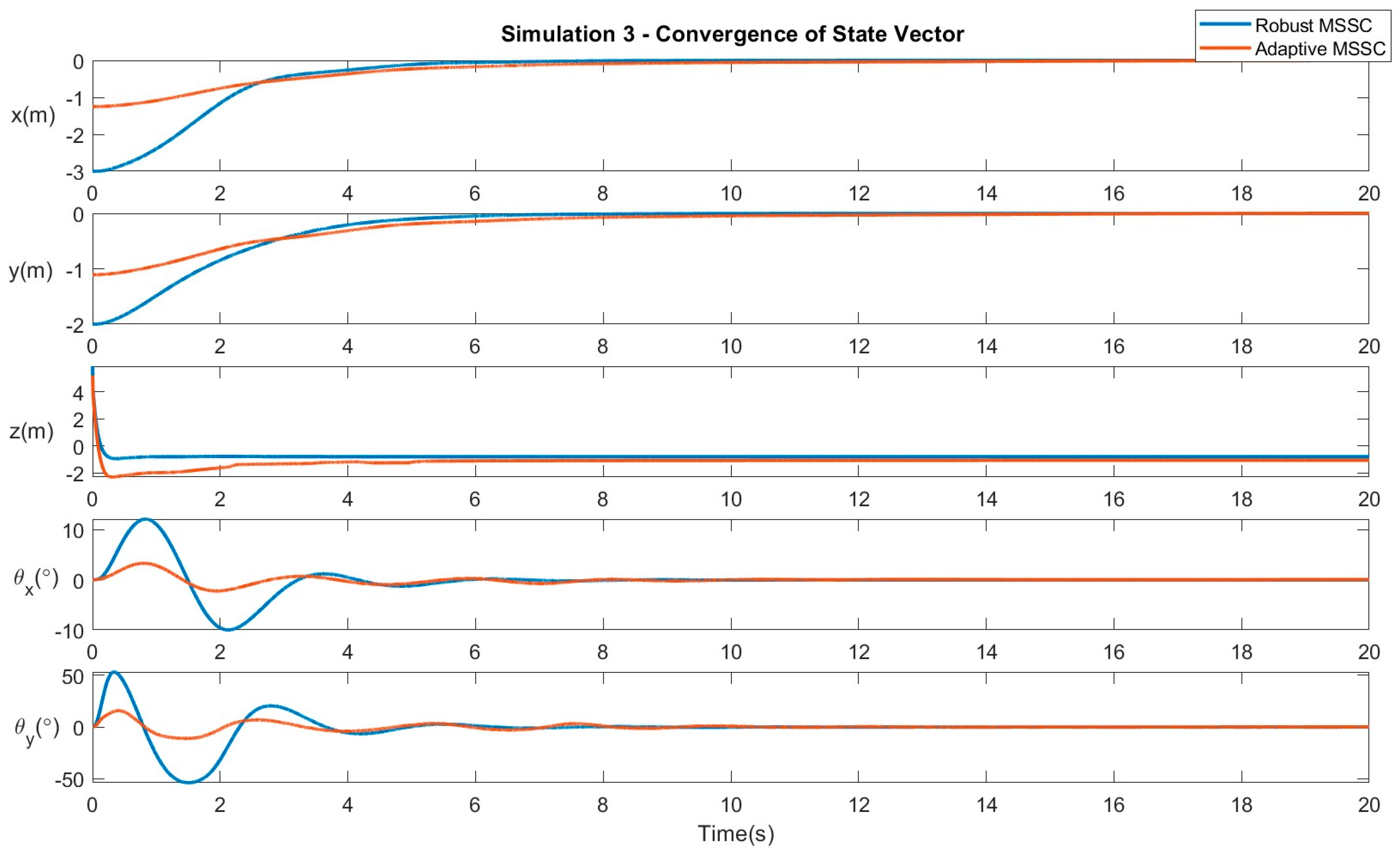
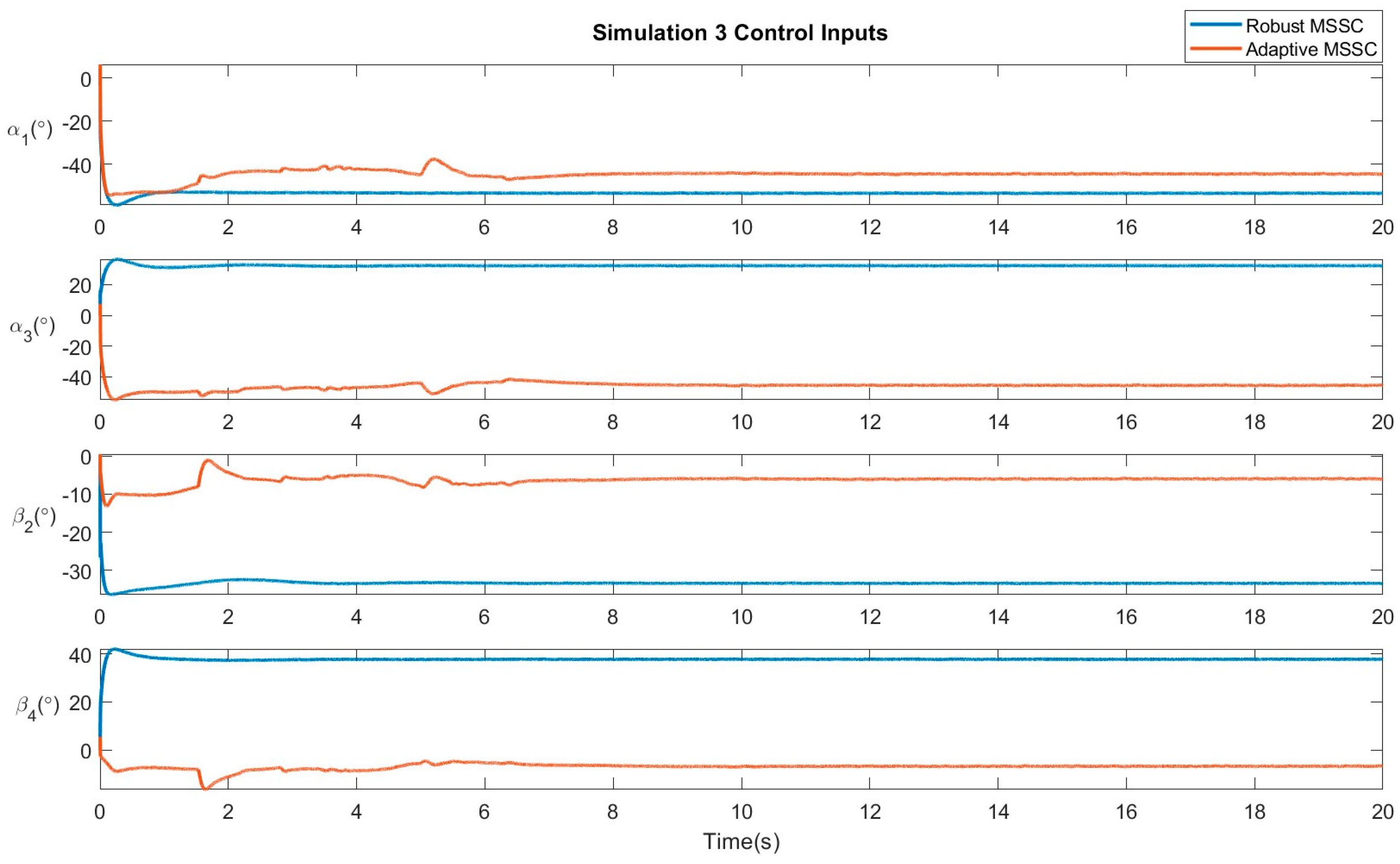
Simulation 3 −Linear movement in the presence of a consistent disturbance vector (impulse): The drone here follows the same path as in the first scenario, but in the presence of an impulse disturbance vector acting along the co-ordinate axes, which is an addition to the dynamic model of the system. The disturbance vector is defined by
where rand() represents a random disturbance vector.
Figure 6 verifies the convergence of the system states to the desired position.
Figure 7 displays the control efforts necessary for the robust and adaptive variants of the proposed controller.
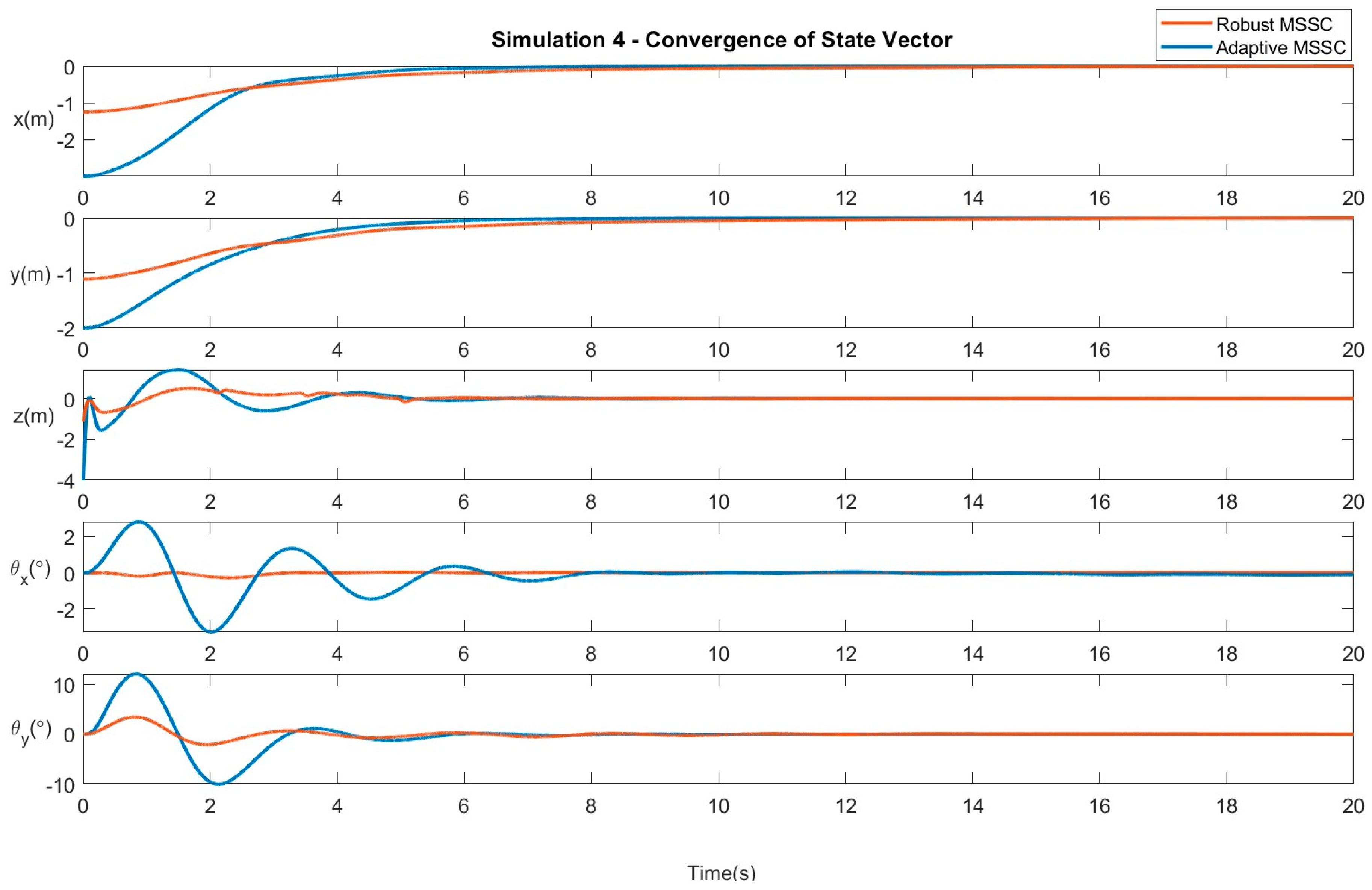
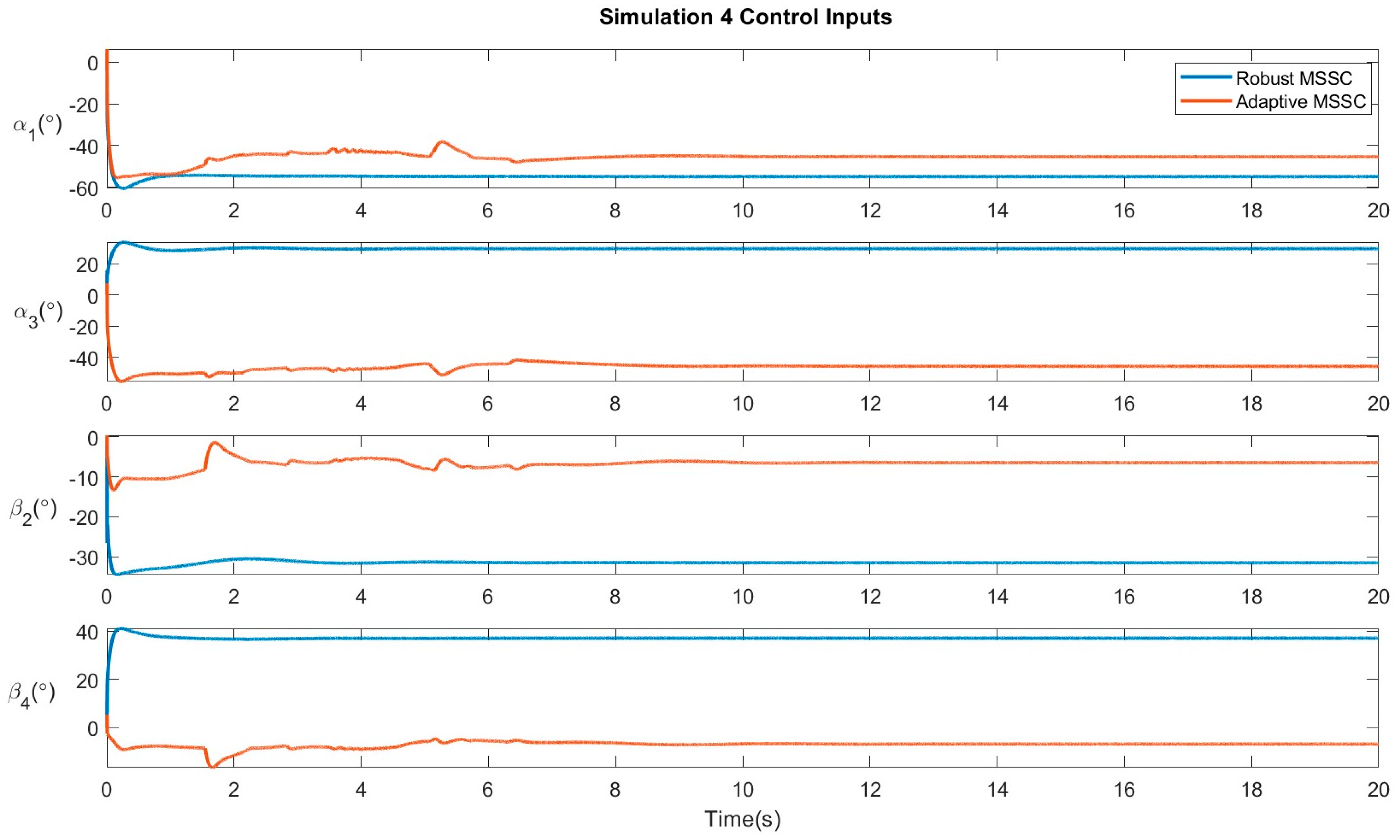
Simulation 4 −Random Disturbances at unspecified time intervals (intermittent disturbances): In the final simulation, the system is subjected to event-triggered disturbances, which are introduced at non-uniform time intervals. The magnitude of these disturbances is variant in nature, ranging from −5 × rand(1) to 5 × rand(1) along each of the co-ordinate axes.
Figure 8 verifies the convergence of the system states to the desired position.
Figure 9 displays the control efforts necessary for the robust and adaptive variants of the proposed controller.


