1. Introduction
The development of an aircraft that combines the advantages of both fixed-wing and rotorcraft, to overcome their weakness, has prompted the creation of a wide variety of new aircraft designs, which have been classified as hybrid VTOLs (H-VTOLs). This type of aircraft offers several advantages over the traditional ones, since its VTOL capabilities eliminate the need for runways, enabling it to operate in confined spaces or remote areas, and providing enhanced versatility [
1,
2]. Zong et al. [
3] mentioned that the primary focus of developing this type of aircraft revolves around urban air mobility applications, given the potential to effectively and safely handle urban transportation needs. Furthermore, prominent organizations such as NASA and Uber are considering how the utilization of H-VTOLs could bring revolutionary changes in industries such as transportation, search and rescue, package delivery, and security patrols.
Despite their advantages, H-VTOLs also face challenges that require further research and development, such as the need for additional power to conduct vertical take off, compared with the power required for the fixed-wing phase. This increased power demand can affect the overall efficiency and endurance of the vehicle, limiting its flight time or its payload capacity. In this sense, the key points that must be taken into account in the design of these vehicles include the addition of dead weight; the requirement for higher speeds, which might not be achieved if the same propulsion system is used for both flying phases; the fact that VTOL efficiency means greater lift and less required power; the fact that cruising efficiency means greater lift and less drag; and, finally, the need for safer aircraft, seeking to reduce the number of accidents, at least compared with the number of accidents with conventional aircraft [
4].
Nowadays, there exist many configurations of H-VTOLs, which are mainly classified as compound aircraft, tilt-rotor, tilt-wing, tail-sitter, lift-fan, and vectored-thrust vehicles [
5]. These types of configurations are clearly exemplified by the Jump 20 [
6], a compound aircraft with a conventional plane configuration that includes a dedicated quadrotor system for multirotor flight; the Quantum Systems Tron F90 [
7], a tilting-rotor aircraft, similar to the Jump 20 UAV with the addition of a tilting mechanism that uses the same propulsion system for vertical and cruise flight; the JAXA’s QTWUAV AKITSU tilt-wing [
8], which consists of tandem tilting wings and propellers mounted on the leading edge of each UAV wing; and the WintraOne [
9], a tail-sitter UAV with two propellers that allow taking-off vertically and a mechanism to tilt the whole airframe forward for cruise flight. All of these aircraft address the issue of the extra power consumed during multirotor flight by reducing the dead weight through using the same propulsion system for all phases of flight, with the exception of the compound aircraft whose main advantage lies in separating each propulsion system, in order to optimize them for each phase of flight.
Alternatively, in order to increase the VTOL efficiency of the H-VTOl aircraft, the distributed electric propulsion (DEP) technique integrates the propulsion system from multiple small-size engines and propellers instead of using a large motor with an equally large propeller. In this technique, propulsion units are distributed on the frame to stabilize the attitude of the aircraft, which features a higher propulsion efficiency [
10,
11,
12]. The effectiveness of this technology has been demonstrated by Kim et al. [
13], where the authors employed DEP on a NASA demonstration aircraft, a conventional take-off and landing vehicle (CTOL) called X-57. This aircraft was reconfigured with a much smaller wing than the reference aircraft Tecman P2006T. Such a smaller wing was achieved thanks to the lift provided by 12 small electric propellers along the leading edge of the wing during the take-off and landing phases of flight [
14].
Similarly, the Joby S2 concept incorporates DEP technology, positioning its engines throughout the aircraft, without increasing mechanical complexity and weight. This aircraft incorporates twelve motors with twelve fixed-pitch rotors. During aircraft mode, the induced velocity generated by the rotors, which become propellers, provides the vehicle with a lift-enhancing effect, similar to that produced by hyper-sustainable mechanisms, as demonstrated by Stoll et al. [
15]. The Greased Lightning GL-10 vehicle, a joint effort of the Advanced Aircraft Company and NASA is an aircraft that incorporates 10 rotors for multirotor flight, which subsequently change to propellers through a tilting system, to propel the vehicle as a fixed wing [
16]. The Langley Aerodrome 8 is a tandem tilt-wing electric VTOL configuration that has two tilt wings, eight electric motors, and several control surfaces, for a total of twenty independent control actuators. This aircraft is utilized for testing and evaluation of new technologies for H-VTOL vehicles, such as the examination of new developments in DEP, advanced flight control systems, and complex aerodynamics [
17].
1.1. Related Work
In 2016, the Lilium company conducted a flight test of its all-electric two-passenger VTOL vehicle. This aircraft consists of thirty-six ducted fans mounted along its 10 m wingspan. When taking-off, the engines are pointed downwards, to produce lift, and then the engines rotate to the horizontal position to produce thrust for the aircraft mode [
18]. Similarly, the Lightning Strike VTOL X-Plane, an aircraft that began as a project by DARPA, features twenty-four electric ducted fans distributed across the vehicle’s wingspan and canard surface, whose functionality was validated through conducting flight tests with a scaled-down version [
19]. In 2018, Zhao and Zhou [
20] presented a lift-propulsion VTOL concept, which adopted the idea of the supporting body incorporating the fuselage as a lift element and the wing section. The drive unit composed two main ducted fans at the wingtips and another two at the rear of the fuselage, to generate thrust in airplane mode. They presented the aircraft design, the prototype construction, and vertical flight tests. In [
21], Hoeveler et al. developed a fan-in-wing VTOL using two ducted fans in the wing. In their design, the authors incorporated a step for each ducted-fan outlet at the bottom of the wing, in order to obtain a better performance during airplane mode. This vehicle has a tilting ducted fan on the front, used to perform the transition in flight. In their research work, the geometry of the duct with the added step was analyzed and compared against a wing with a standard duct and a wing without ducts. The lift/drag relation for the three studied cases showed an increase of up to 66% when the step at the bottom of the wing was used. However, the performance with respect to the ductless wing characteristics was considerably improved.
In this research work, two H-VTOL concepts are presented: the XEVTOL-2FNW and XEVTOL-4FNW. The two experimental vehicles consist of a flying wing aircraft with a tilting system incorporated at the front for the flight transition and one or two rotors embedded in the wing, according to the 2FNW or 4FNW configuration. These concepts deal with the extra power demanded during the VTOL phase using a tilt-rotor configuration, which reduces the dead weight through using the cruise propulsion as a lift system during multirotor flight. The DEP technique was employed, together with the incorporation of ducted-fans to increase the efficiency of the propulsion system during the VTOL phase, and we performed a comparison of the 2FNW and 4FNW concepts, making use of model-in-the-loop (MIL) simulations. The aim of these simulations was to evaluate the performance of the aircraft when the required thrust is distributed throughout a different number of ducted-fans and, simultaneously, to evaluate their effects on the aerodynamics of the aircraft.
1.2. Main Contributions
The main contributions of this work can be summarized as follows:
A mathematical model of two unconventional H-VTOLs was derived, to obtain the corresponding flight controllers;
An evaluation is presented regarding the advantages and drawbacks of using 4 or 6 ducted fans during the cruising phase by conducting a study of the performance of the two platforms based on MIL simulations using X-Plane flight simulator and Matlab.
The remainder of this paper is organized as follows:
Section 2 presents the XEVTOL-2FNW and XEVTOL-4FNW concepts, proposed to reduce energy consumption and to increase the lift produced by the rotor during multirotor flight and incorporating DEP technology, as well as a description of the dynamic model of the XEVTOL-2FNW using the Newton–Euler formulation, considering the forces generated by the rotors, as well as the aerodynamic forces and moments generated by the aircraft wing.
Section 3 presents a 3D model of the two aircraft concepts developed on Plane Maker and the flight controllers implemented for the model-in-the-loop simulations using the X-Plane flight simulator and Matlab-Simulink.
Section 4 shows the simulation results of the two vehicles, and the energy parameters of the aircraft are compared to evaluate the advantage of the DEP and the drawbacks of increasing the number of ducted fans. Finally, concluding remarks about this research are provided in
Section 5.
2. Mathematical Model of the XEVTOL-2FNW
The XEVTOL-2FNW and XEVTOL-4FNW aircraft concepts are based on DEP technology, which states that it is more efficient to have several light small engines, distributed along a vehicle than having a single powerful but heavy engine. This implies that the engines operate in a more efficient region, where they generate more lift with a lower energy consumption (g/W). In addition, ducted fans were utilized for thrust generation in multirotor flight, to improve the energy efficiency of each rotor and provide an additional layer of safety since the blades are enclosed within the housing provided by the ducts, reducing the risk of injury or damage to surrounding objects or people in close proximity to the aircraft [
22,
23,
24]. The design of both aircraft concepts was based on the commercial UAV Mapper V1.8, manufactured by TUFFWING [
25], a flying wing with a wingspan of 120 cm.
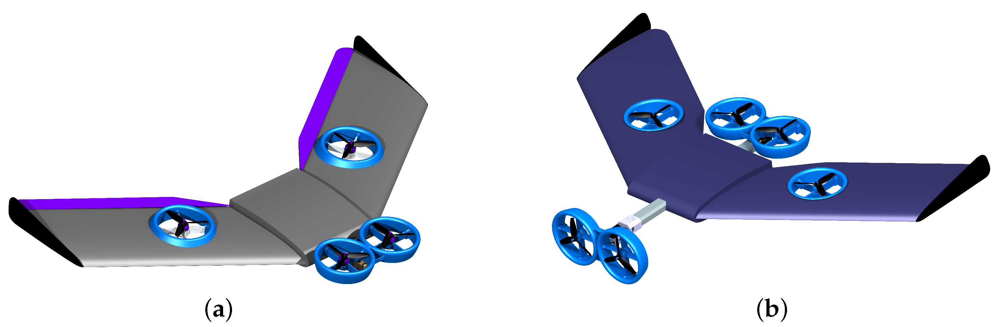
Based on the above considerations, the proposed XEVTOL concepts can be defined as a flying wing aircraft with a dedicated lift system of ducted fans in the wing, with a tilting dual-ducted fan on the front of the aircraft for the transition phase (see
Figure 1). The XEVTOL-2FNW concept incorporates two ducted fans embedded in the wing and a tilting dual-ducted fan in the front of the vehicle. The tilting ducted fans allow carrying out the transition from the multirotor to the fixed-wing mode and vice versa. In the fixed-wing phase, two elevons, acting as the elevator and the aileron, are the control surfaces. For the XEVTOL-4FNW, two ducted fans were added at the rear of the vehicle, which required increasing the distance of the tilting dual-ducted fan from the fuselage, in order to counterbalance the torque of the rear ducted fans.
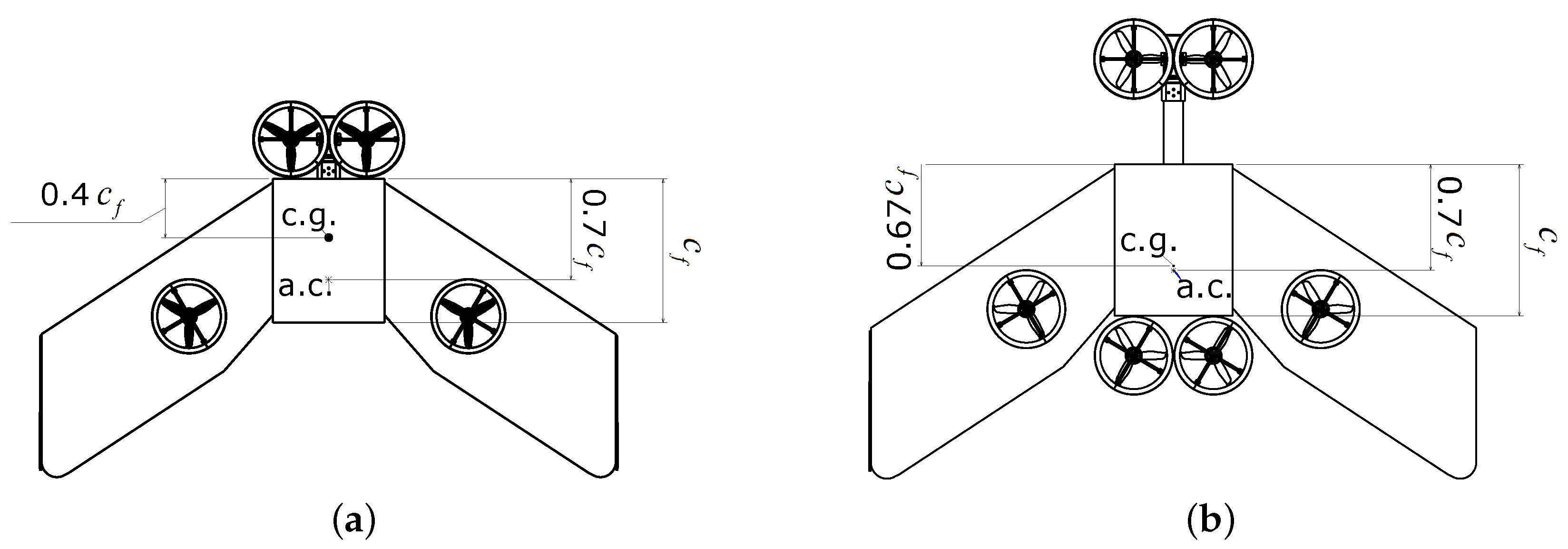
Furthermore, the addition of two rear ducted fans to the XEVTOL-4FNW configuration primarily altered the center of gravity (c.g.), the MTOW of the platform and, to a minor degree, the aerodynamic center (a.c.), given that the latter is more influenced by the characteristics of the wings. The c.g. of the XEVTOL-4FNW is located at 40% of the fuselage chord, while for the XEVTOL-4FNW it is located at 67% of the fuselage chord. The empty weight for the XEVTOL-2FNW is 2.1 kg, while for the XEVTOL-4FNW configurations it is 2.7 kg.
Figure 2 depicts the location of the c.g and the a.c. for both platforms.
MIL simulations were utilized to evaluate the effects of incorporating the additional ducted fans on the vehicle’s performance during the VTOL phase. The XEVTOL-2FNW and XEVTOL-4FNW concepts were introduced to assess factors such as energy efficiency, power consumption, and lift and drag forces. In this sense, the development of the mathematical model is described below, in order to obtain the corresponding flight controllers to be implemented in the MIL simulations.
The mathematical model of XEVTOL-2FNW was derived using the Newton–Euler formalism. To this end, in addition to the forces generated by the rotors, the contribution of the aerodynamic forces and the moments generated by the aircraft wing was considered.
2.1. Dynamics
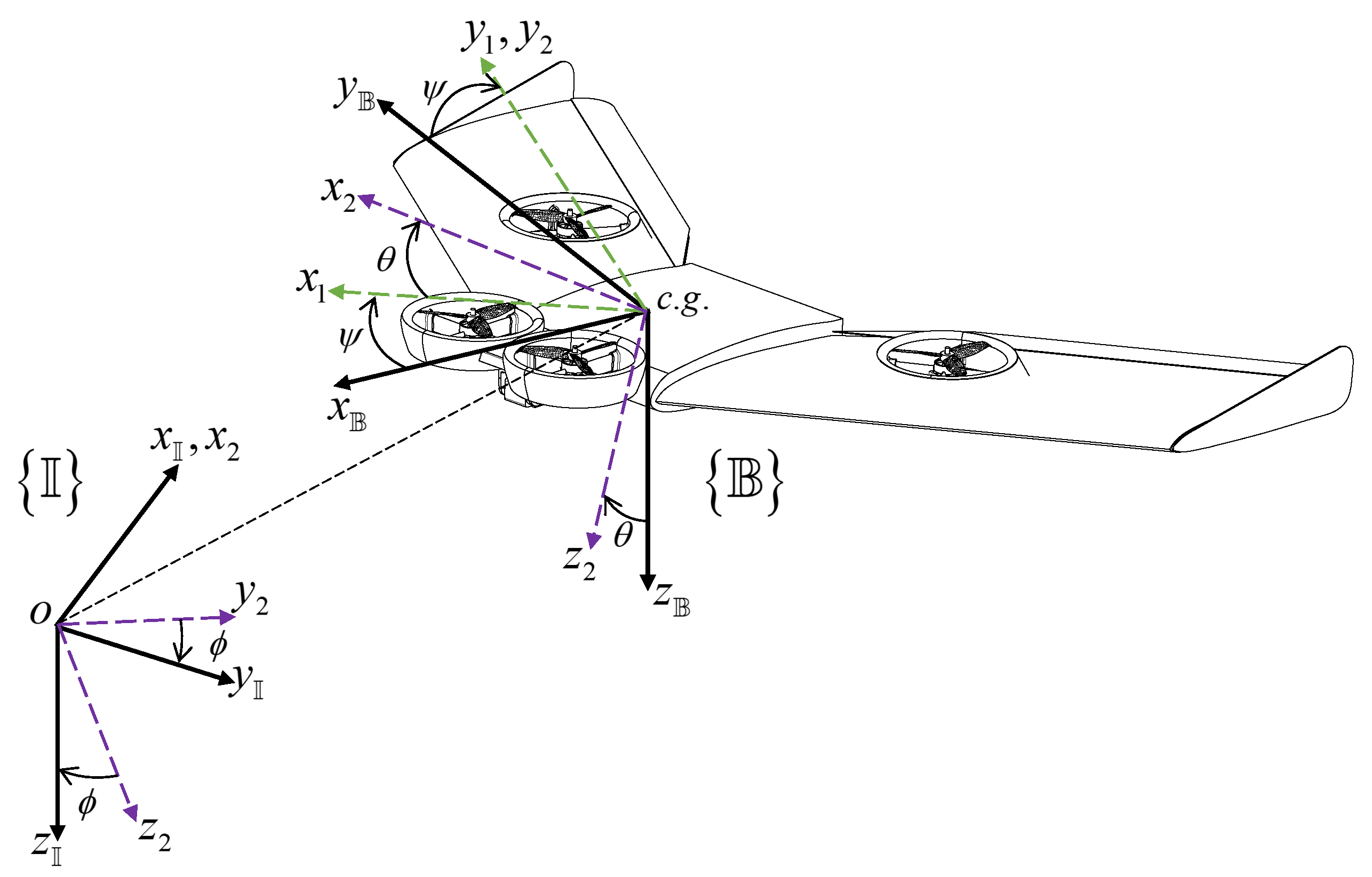
Consider the XEVTOL-2FNW aerial platform as a rigid body with six degrees of freedom with a body frame
located at its c.g. and an inertial frame
fixed in the earth as shown in
Figure 3.
The mathematical model of the aircraft was derived using the Newton–Euler formalism [
26] as:
where
m is the mass of the aircraft, and
and
are the identity matrix and the zero matrix, respectively. The linear velocity in the body frame is denoted by
, where
represent the linear velocity about the
axes, respectively, and whose derivative with respect to time is denoted as
. The angular velocity in the body frame is given as
, where
p,
q, and
r represent the rate of change in the pitch, roll, and yaw angle expressed in the body frame, respectively. The derivative with respect to time of this angular velocity is denoted as
.
and
represent the forces and moments on the body frame acting on the c.g. of the aircraft. The matrix
is the inertia tensor that contains the vehicle’s moments of inertia. Since the
-
plane is symmetric,
and
[
27], and the inertia tensor is defined as
Equation (
1) is defined in the body frame {
} and it has to be transformed to the inertial frame {
}, in order to obtain the mathematical model in terms of the inertial frame. This is done by performing axis rotation, first rotating about the
axis a yaw angle (
). Then, rotating about the
axis a pitch angle (
). Finally, rotating about the
axis a theta angle (
. Obtaining the
matrix, which is an orthogonal rotation matrix leading from the body frame to the inertial frame [
28], is given as:
where
and
.
While the matrix
gives us the equation for the rotational kinematics as a function of the angular velocities [
28], which is given by
Then, by grouping Equations (
3) and (
4), the transformation that permits the transfer of linear and angular velocities and accelerations from the body frame to the inertial frame is obtained. Equation (
5) presents the transformation of linear and angular acceleration from the body to the inertial frame:
The linear acceleration vector in the inertial frame is defined as , while the angular acceleration vector in the inertial frame is .
2.2. Forces
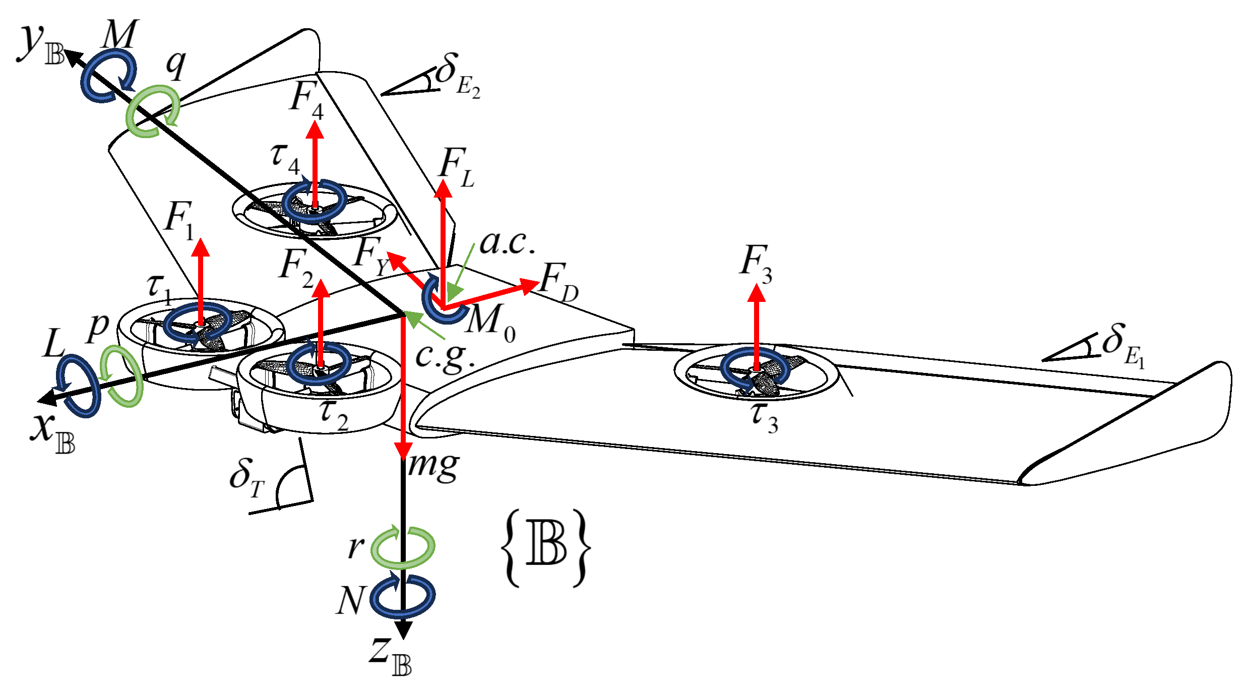
Figure 4 depicts the forces (red arrows) and moments (blue arrows) in the body frame, the c.g. of the body on the diagram, and the a.c. and the origin of the inertial frame {o}. The total force on the vehicle given in Equation (
6) is expressed as
, and this is given by the vector sum of 3 types of forces: the propulsion forces
due to propellers/rotors, the aerodynamic forces
due to the wing, and the gravitational force
.
2.2.1. Propulsion Forces
The propulsion forces generated by the vehicle are denoted by Equation (
7). Where
,
define the thrust forces of the prop/rotors,
k is a proportional constant, and
is the angular velocity of the motor. The thrust forces due to the front ducted fans (
and
) have a contribution to the body frame
or
, depending of the tilting angle
[
26]. It can be observed that the ducted fans
and
only make a contribution in the vertical axis
.
Note that for the multirotor mode and for the fixed-wing mode.
2.2.2. Aerodynamic Forces of the Wing
The aerodynamic forces are mainly due to the interaction of the wing with the wind, generating the lift force
, the drag force
, and the lateral force
, as defined in Equation (
8):
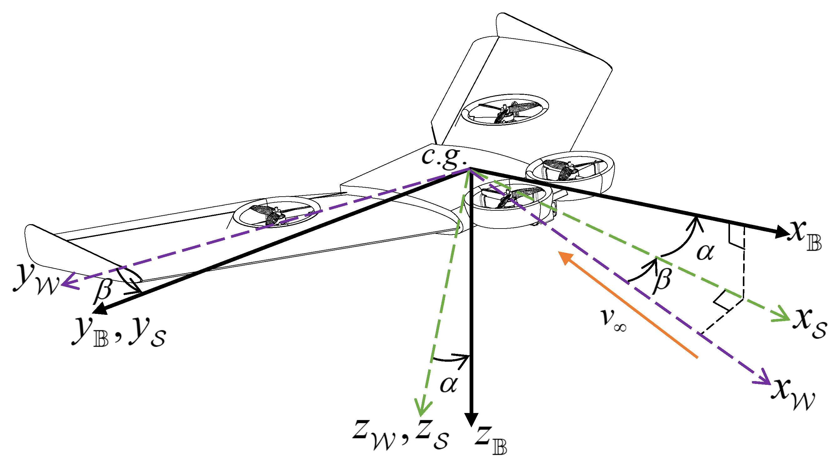
The rotation matrix
in Equation (
9) allows these aerodynamic forces to be transformed from the wind reference frame to the body frame [
29], by performing rotations of the wind frame
about the
with a slip angle
and a rotation of the stability frame
about the
and incidence angle
, as shown in
Figure 5.
which can be written as
where
is the wing density;
is the relative wind speed,
S is the wing surface;
is the wing drag coefficient;
is the wing drag coefficient at zero lift;
is the drag coefficient due to wing lift;
is the lateral force coefficient;
is the lift coefficient of the wing;
,
, and
,
are the aerodynamic coefficients;
is the angle of deflection of the elevon; and
is the elevon trim [
30,
31].
2.2.3. Gravitational Force
Since, in Equation (
6), the force of gravity is defined in the inertial frame
, a rotation is performed as a function of the Euler angles
and
, in order to transfer this force to the body frame
using Equation (
11), where
m/s
is the gravitational acceleration.
2.3. Moments Acting on the Aircraft
The moments acting on the platform are due to the propulsion systems
, the gyroscopic effect
, and the aerodynamics moments
, whose total sum is denoted as:
2.3.1. Propulsion Moments
The moments generated by the propulsion system are given by two phenomena. The first is due to the force generated by the motors because of their position with respect to the c.g. and are denoted as
. The second results from the torque produced by the motors during their rotation and is denoted as
. Combining these two expressions, the moments due to the propulsion system are given as
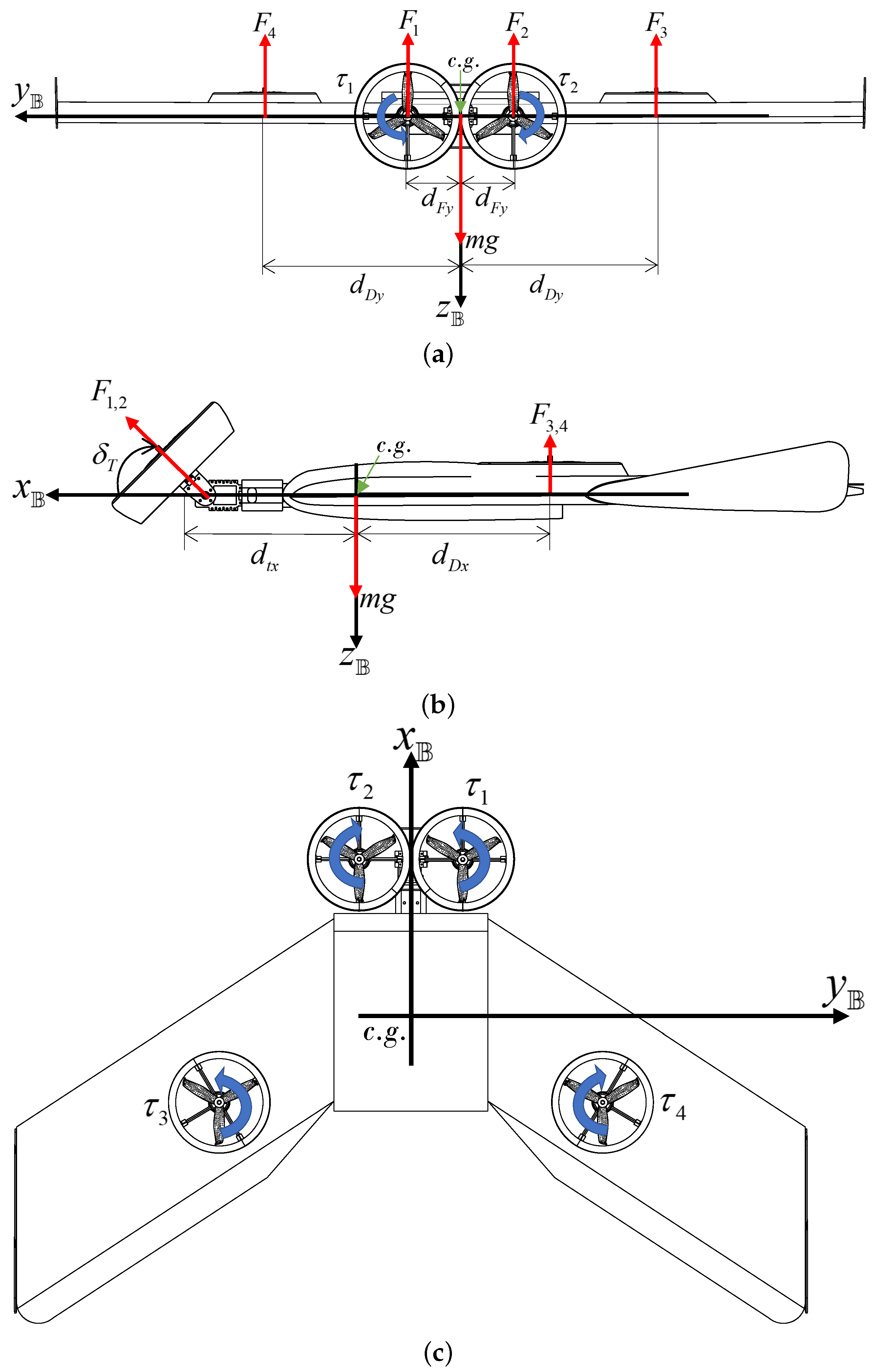
Figure 6 shows the body diagrams used for the analysis of the moments about the three axes of the vehicle (
,
,
), which are given by:
where
,
1, 2, 3, 4 is the torque generated by the motors and
is a proportional constant used to relate the force generated by the motors with the torque they produce [
26].
2.3.2. Gyroscopic Moments
The gyroscopic moments of the propellers are given in Equation (
15). In the first term of the right hand side of Equation (
15), i.e., inside the vector product between the angular speed of the body and each motor, a rotation of each motor is modeled as a function of the tilting angle
, which applies only to motors 1 and 2, since they change their gyroscopic moment contribution depending on their orientation, due to the variation of the
angle, while motors 3 and 4 remain fixed to the body:
where
,
is the moment of inertia of the propellers about the axes of rotation of the engines [
32].
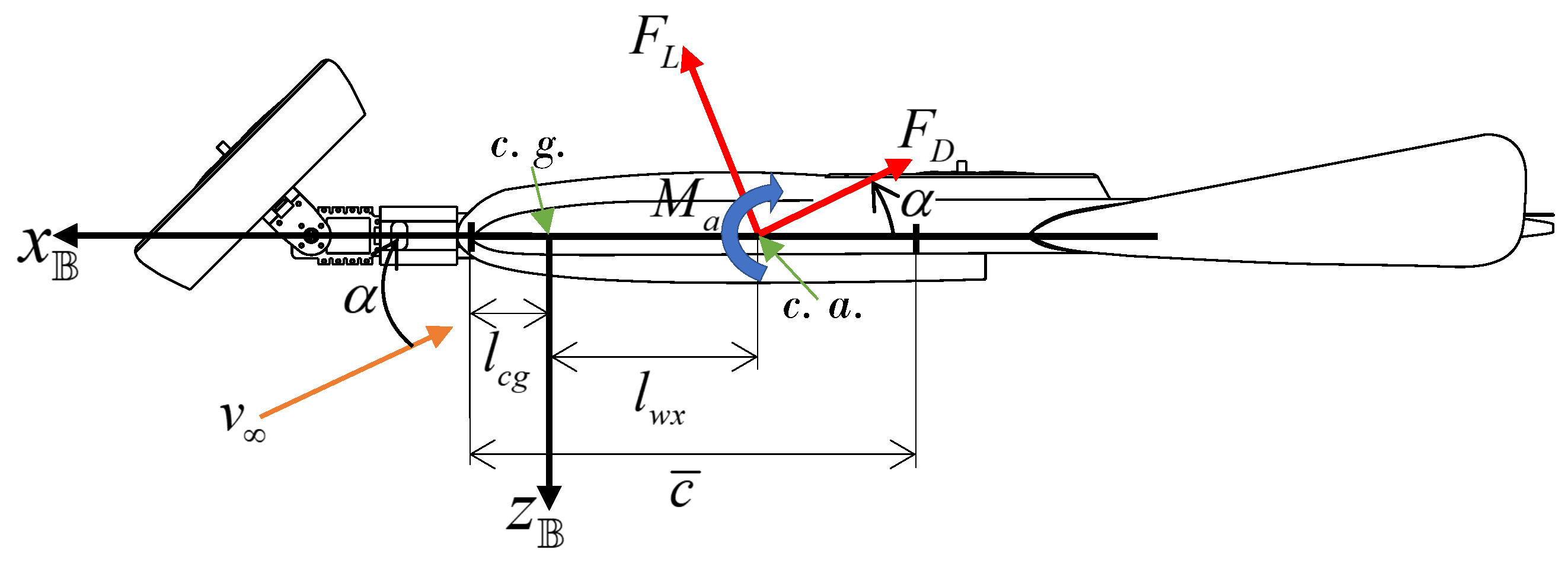
2.3.3. Aerodynamic Moments
For delta wing aircraft, the moments are generated exclusively by the aerodynamic effects of the wing, since they lack the stabilizing surfaces present in conventional aircraft. This contribution of aerodynamic moments is linked to the wing coefficients. The aerodynamic moments of the aircraft are expressed by the Equation (
17), derived from the diagram shown in
Figure 7. These moments result from the aerodynamic forces
, acting at a distance
from the a.c. to the c.g.
As shown in
Figure 7, the aerodynamic moments that act on the vehicle are determined by the aerodynamic forces and the distances to the c.g. (
) and to the c.a. (
) from the mean aerodynamic chord (
) of the wing, and they are given as follows:
where
is the position vector of the a.c. in the body frame,
b is the wingspan,
is the mean aerodynamic chord, and the vector
represents the aerodynamic moments as a function of the dimensionless aerodynamic coefficients
,
and
[
33].
2.4. Equations of Motion
From the Newton–Euler formulation, it can be observed that the equations of motion of the XEVTOL-2FNW for the multirotor, transition, and fixed-wing modes are given as
Equations (
19) and (
20) represent the linear and angular velocities of the vehicle with respect to the inertial frame, while Equations (
21) and (
22) represent the linear and angular velocities referring to the body axes.
Since the XEVTOL-4FNW configuration is similar to the one developed in this section, the derivation of its mathematical model is omitted for brevity. The main difference between the two configurations is in the forces and moments acting on the vehicle, due to the addition of another two ducted fans in the XEVTOL-4FNW configuration. In this sense, only the corresponding terms of forces and moments for the propulsion system will be modified.
Multirotor Flight Mode Simplification
During multirotor flight, the tilting engines are in the vertical position
, with an incidence angle
and a slip angle
. The aerodynamic forces and moments are neglected, i.e.,
and
. For hovering flight conditions, the vehicle’s roll, pitch, and yaw angles have small variations, so the angular velocities can be considered as
,
q,
≈
, 0,
. Since
,
q,
, 0,
and the inertia of the propellers is small, the gyroscopic effects of the propellers are neglected. Considering the body axes coincide with the main axes of the vehicle, the inertia product
is zero [
29]. Applying these considerations to Equations (
19)–(
22), the dynamic model for multirotor flight yields
where
is control force and
,
, and
are the control moments.
3. Model-in-the-Loop Simulations in X-PLANE
Testing control algorithms in a physical aircraft is an expensive and time-consuming process that requires many repetitive tests during the development phase. In addition, current UAV regulations are too restrictive, since experimental testing is a dangerous task. Moreover, a possible failure of the aircraft sensors could cause the estimates made by the vehicle to be inaccurate. This does not allow correct evaluation of the control algorithms and other systems during flight tests. Therefore, a common alternative for flight validation is to develop flight tests using virtual environments by performing model-in-the-loop (MIL) simulations [
34].
MIL simulations refer to a type of simulation where a mathematical or computational model is incorporated into a closed-loop system. The model interacts with other components of the system, such as sensors, actuators, and control algorithms, to simulate the behavior of the overall system. In MIL simulations, the model is typically a simplified representation of the real system, often developed using mathematical equations or computer-based algorithms. The purpose of using a model is to simulate the system’s behavior under various conditions, test different control strategies, or evaluate the performance of specific components [
35].
In this sense, MIL simulations were employed to evaluate and compare the performance of the two XEVTOL concepts. The position and attitude of the XEVTOL concepts were obtained using the software X-Plane, which is a flight simulator developed by Laminar Research with realistic flight physics. This allowed us to verify, in this case, the XEVTOL concepts, providing pivotal feedback for the design phase and for the design of control strategies, and obtaining simulation results of the aircraft performance close to a flight in real conditions. To this end, X-Plane utilizes blade element momentum theory (BEMT) to analyze the geometric configuration of an aircraft and computes its flight behavior. This approach involves subdividing the aircraft into smaller elements and continuously calculating the forces acting on each element. These forces are then translated into accelerations, which are integrated over time to derive the aircraft’s velocities and positions, to describe the dynamics of the aircraft motion in the simulation [
36].
Thong [
37] tested the accuracy of X-Plane by means of a series of simulations with a model of a F-15E. They concluded that the simulator was accurate in the sense that the input parameters were captured as close to reality as possible. Moreover, the information obtained through the simulations was compared with that obtained both analytically and from the aircraft flight manuals. Similarly, Fayyaz [
38] developed simulations with the Pilatus PC-9 modeled in X-Plane 10 with the least number of discrepancies with respect to the real aircraft. The simulation results were compared with theoretical and real data, showing that the performance and stability characteristics of the aircraft remained within a range of ten percent compared to the theoretical/actual values, with the exception of lateral stability.
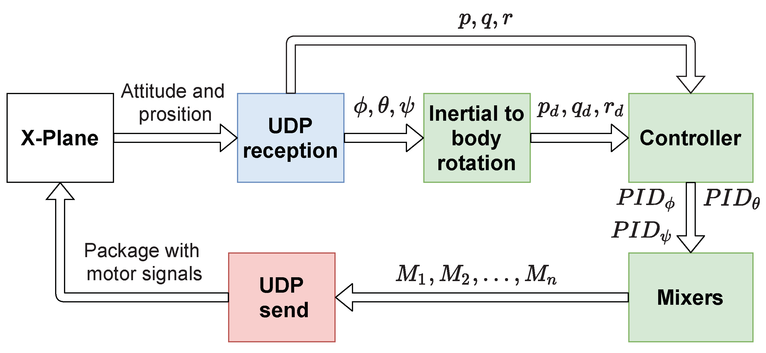
In our simulation environment, the scheme used to conduct MIL simulations used X-Plane and Matlab-Simulink. In this case, the X-Plane program was in charge of generating the dynamic model of the vehicle from a 3D model developed in Plane Maker software. The position and orientation of the vehicle was sent to Simulink through the UDP protocol. Once in Simulink, this information was used to compute the corresponding flight controllers and, finally, the obtained control signals were sent to the vehicle engines in X-Plane for the operation of the vehicle.
Figure 8 schematizes this simulation process.
The development of the 3D model of the XEVTOL concepts in Plane Maker, as well as the control scheme used for the development of the MIL simulations, are described in
Section 3.1.
3.1. Plane Maker 3D Model
Plane Maker is the software part of X-Plane that allows users to create and edit their customized aircraft, based on existing models or entirely new designs. By setting different physical attributes such as the weight, wingspan, control surfaces, propulsion system, and wing profile, among others, users can define the characteristics of their custom aircraft. Once the model has been developed and imported into X-Plane, the software estimates and simulates how the aircraft would perform in real conditions [
39].
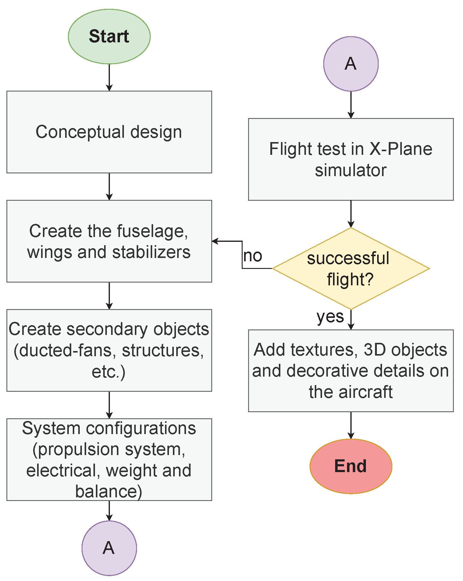
The design methodology used to obtain the 3D model of the aircraft in plane maker is presented in the diagram in
Figure 9. This corresponds to the design of the XEVTOL-2FNW concept; however, the same methodology applies for the design of the XEVTOL-4FNW version. The main difference is in the definition of the propulsion system, as two additional engines needed to be incorporated for the XEVTOL-4FNW version.
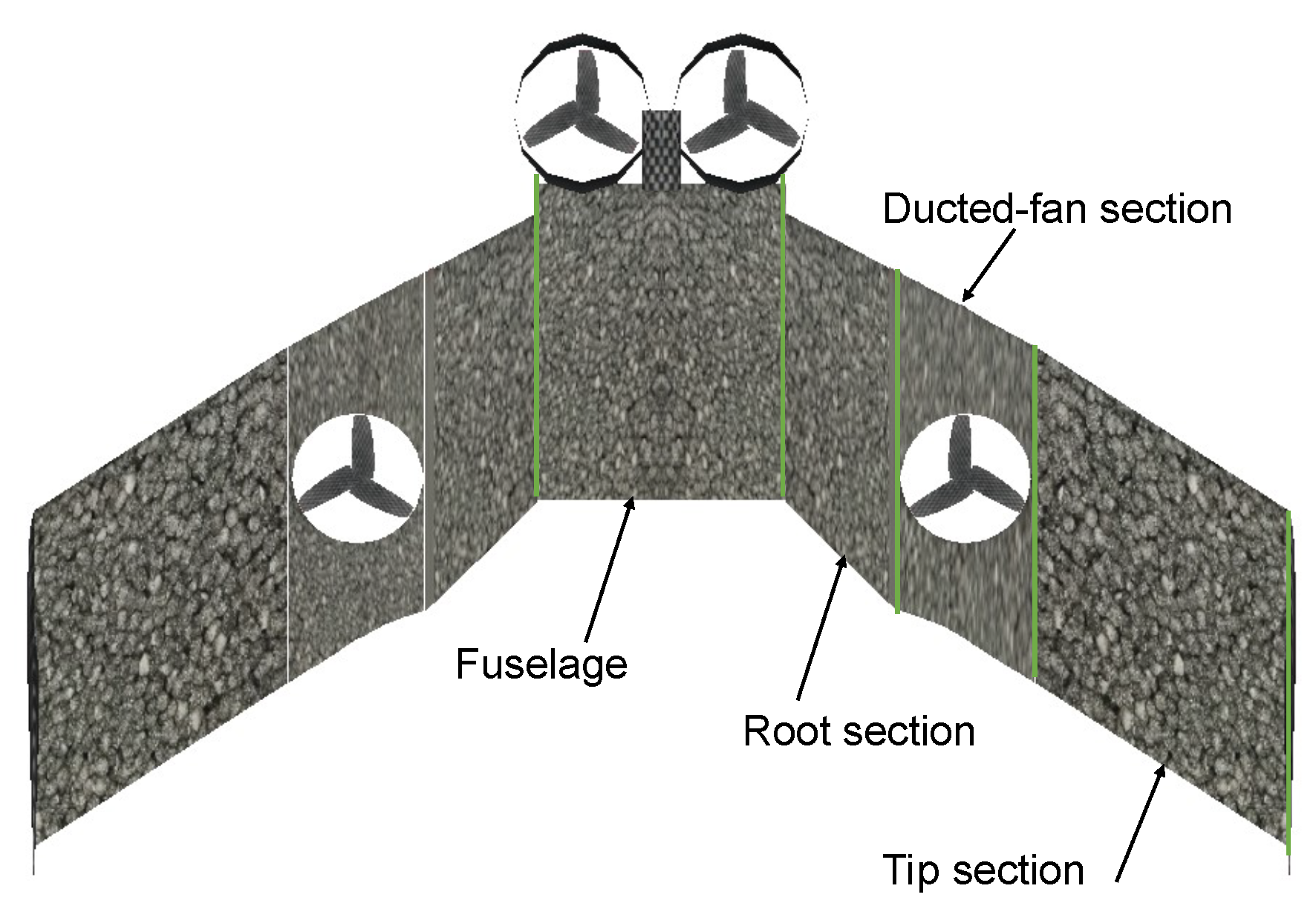
The geometry of the vehicle’s wing was defined in the following way: the central part of the vehicle that serves as the fuselage is part of the aircraft’s wing, so it was modeled like a wing section, considering this section as a rectangular wing. The right semi-wing was considered in three sections, with two wing sections located at the tip and root, and a central part where the ducted-fan is located, as shown in
Figure 10.
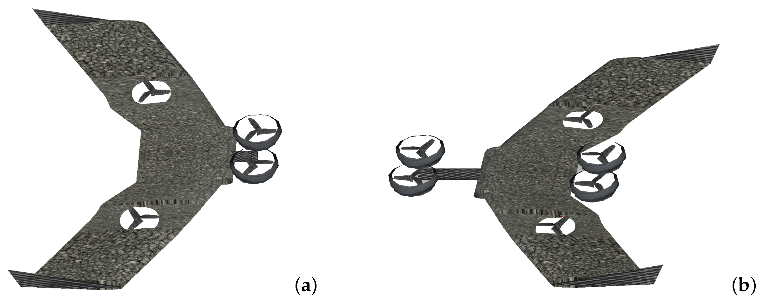
Next, the electrical system was configured in the Systems module within the Standard tab in Plane Maker. The electrical parameters to be used during the simulation were determined, including the source of the electrical energy, the buses through which the energy is distributed, and the inverters. A 59 Wh battery, a single channel, and no inverters were defined. The weight and balance of the aircraft were defined using the module “Weight & Balance” where the location of the c.g. on the longitudinal axis was defined, indicating a maximum and minimum value, and the c.g. on the vertical axis was also indicated; defining for the flying wing a c.g. at 40% and 67% of the fuselage chord, an empty weight of 2.1 kg and 2.7 kg for the XEVTOL-2FNW and XEVTOL-4FNW configurations, respectively. The 3D models of the XEVTOL concepts developed in Plane Maker are shown in
Figure 11.
3.2. Multirotor Flight Control
From the mathematical model for multirotor flight presented in Equations (
23)–(
28), the complete system was divided into four subsystems: the altitude, directional, lateral, and longitudinal subsystems. To control each subsystem, PID controllers were utilized, as described below.
3.2.1. Altitude Controller
The altitude dynamics are given by Equation (
25) as:
then, defining the altitude error
, where
is the desired altitude, the following computation can be performed:
Substituting Equation (
29) into Equation (
30), the following equation is obtained:
. Since the control objective is to guarantee that
, a PD controller is proposed, resulting in:
. Solving for
, Equation (
31) is obtained as
and finally, substituting Equation (
31) into Equation (
29) and considering
as a constant, Equation (
32) is obtained as
where
.
3.2.2. Directional Controller
The dynamics given by Equation (
28) correspond to the directional dynamics represented by the yaw angle. By considering small angle approximations, i.e.,
, Equation (
33) is obtained as
and defining the error in yaw as
, where
is the desired yaw angle, yields
By substituting Equation (
33) into Equation (
34), the following equation is obtained:
. Since the control objective is to guarantee that
, a PD controller is proposed, resulting in
. By solving for
, Equation (
35) is obtained as
and, substituting Equation (
35) into Equation (
33), Equation (
36) is obtained as
where
3.2.3. Lateral Controller
The lateral subsystem is given in Equations (
24) and (
26). By considering small angle approximations
,
,
and substituting
from Equation (
31), the lateral sub-system is rewritten as in Equations (
37) and (
38) as
where the lateral error is defined as
, with
being the desired lateral position.
By substituting Equation (
37) into Equation (
39), the following equation is obtained
. Since the control objective is to guarantee that
, a PD controller is proposed, resulting in
. Solving for
yields that the desired angle to stabilize the lateral dynamics is given as in Equation (
40):
and substituting Equation (
40) into Equation (
37), Equation (
41) is obtained:
Defining the error in roll as
and substituting Equation (
38) into Equation (
42), given as
the following equation is obtained:
. To guarantee the convergence in the roll angle, a PD controller is proposed, and by solving for
, Equation (
43) is obtained as
and substituting Equation (
43) into Equation (
38) yields
where
.
3.2.4. Longitudinal Controller
The longitudinal subsystem is given by Equations (
23) and (
27). Considering small angle approximations
,
, and by substituting
from Equation (
31), the longitudinal subsystem is rewritten in Equations (
45) and (
46) as
where
is the trigonometric function tangent. Defining the longitudinal error as
, where
is the desired longitudinal position, yields
Following the same methodology used for the lateral controller, the desired pitch angle is obtained in Equation (
48) as
and
yields
By substituting Equation (
49) into the dynamic of
given by Equation (
46), the following equation is obtained:
where
.
Finally, the multirotor flight controllers for the translational dynamics are given as:
while for the rotational dynamics, this is given by
From the control law of the roll dynamics given in Equation (
55), it can be observed that
when
; thus, solving the right hand side of Equation (
55) for
, the expression
is obtained. Since
, the following is obtained:
In the same way, Equations (
59) and (
60) are obtained for the pitch and yaw angles:
where
,
, and
are positive constants relating the orientation error with the desired angular velocity. To relate the desired angular velocities of the inertial frame to the desired angular velocities in the body frame, the transformation matrix
is utilized. The angular velocity transformation using this matrix is given as
3.2.5. Control Laws for the Angular Velocities in the Body Frame
In order to guarantee that the desired angles given in Equations (
58)–(
60) can be achieved, the following PID controllers were employed in the body frame:
where
,
, and
,
are positive constants defined heuristically for tuning the corresponding control law.
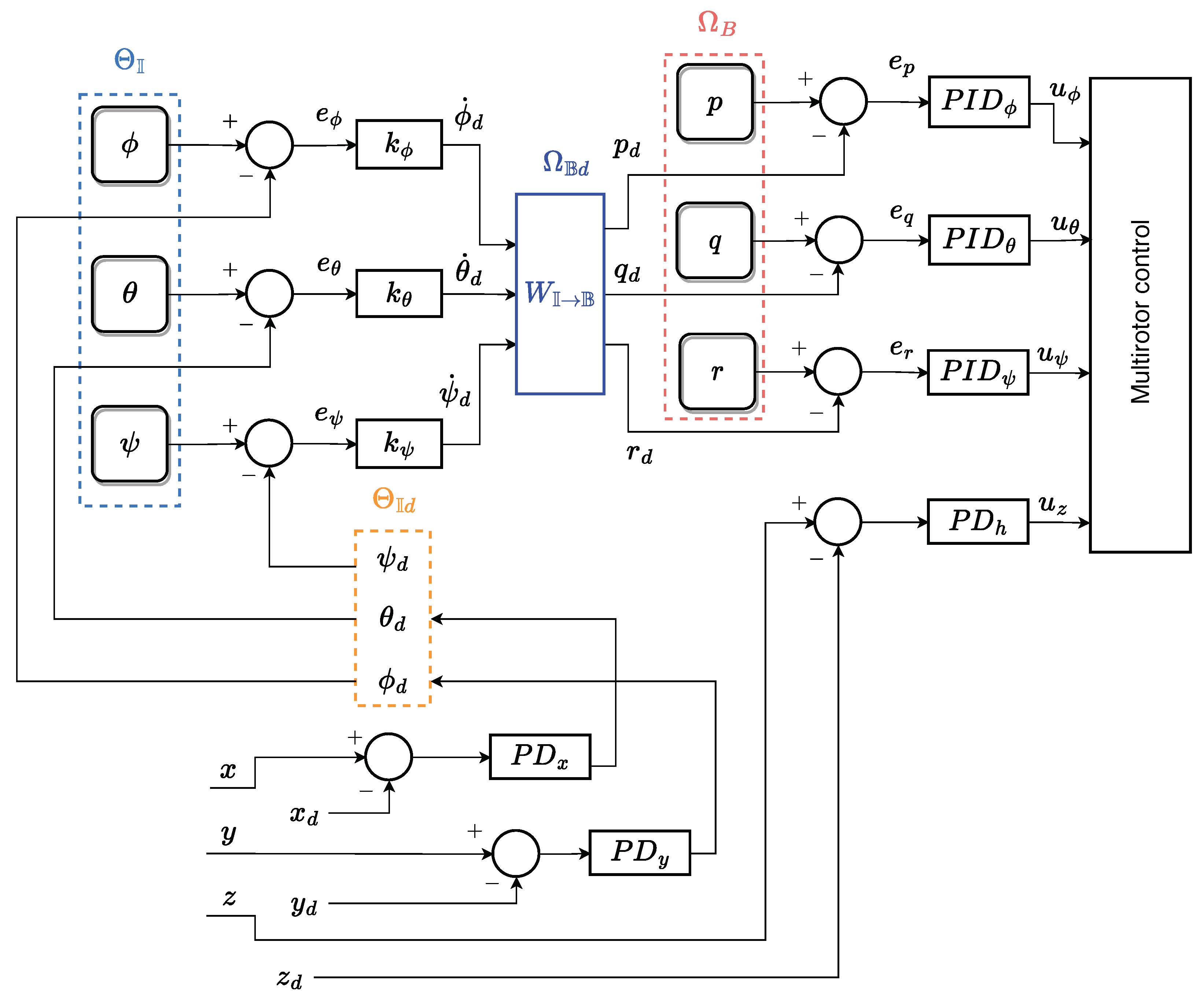
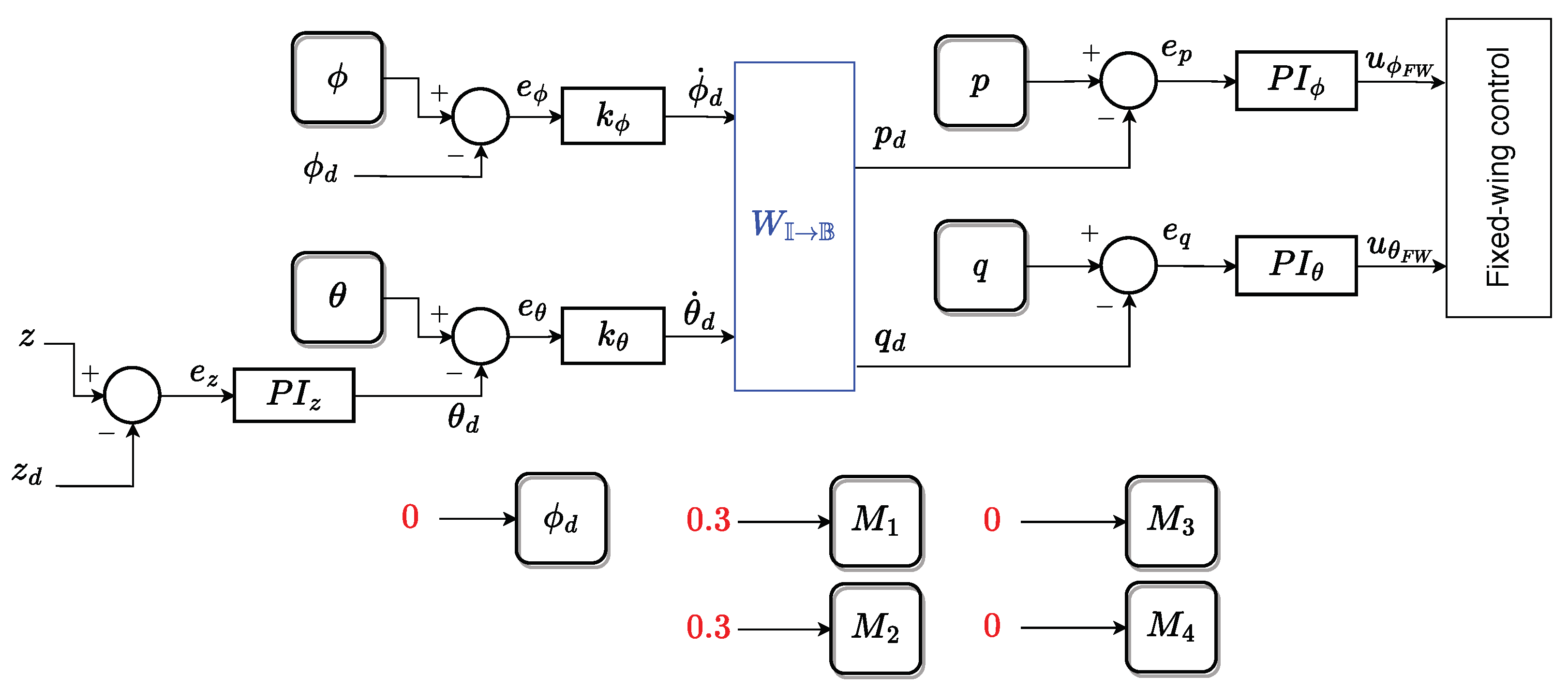
Finally,
Figure 12 shows a block diagram of the control laws for multirotor flight described above.
3.3. Control Schemes for Fixed-Wing and Transition Modes
The control scheme used for the flight phase in fixed-wing mode is shown in
Figure 13. The controllers used during this flight phase were adapted in the PX4 firmware of the Pixhawk autopilot, since the proposed aircraft were not defined in the available configurations of the firmware [
40]. With this control strategy, the dynamics of the roll and pitch angles were stabilized, as well as the aircraft altitude. Note that the desired roll angle is equal to zero, while the desired pitch depends on the altitude error.
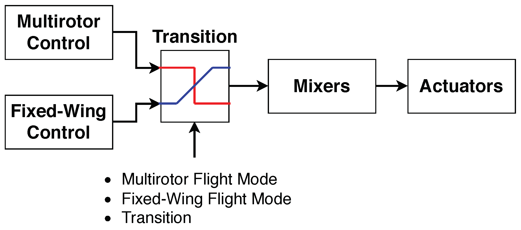
The multirotor and fixed-wing flight mode controllers are activated depending on the desired flight mode. They operate separately or together during the transition. The diagram in
Figure 14 depicts a simplified control diagram of the transition mode. It can be see that, depending on the selected flight mode, a customized mixer is used to send the control signals to the engines and control surfaces of the aircraft in X-Plane.
At the beginning of the flight transition, the aircraft tilts the frontal ducted fans to gain airspeed, while gradually activating the fixed-wing mode controller at the same time that the multirotor controller begins to lose authority, until it is completely deactivated and the vehicle is fully governed by the fixed-wing mode controller.
3.4. Mixers
In order to determine the control signals for each of the engines, the signals obtained from the PID controls are mixed, taking into account the location of the engines with respect to the c.g. of the aircraft, in order to consider the effects that they have on the vehicle dynamics.
The corresponding signal for each engine configuration of the vehicles are defined from the geometry of the aircraft depicted in
Figure 6. Based on such a geometry, the mixers for each motor
of both configurations are given in
Table 1.
4. Simulation Results and Discussions
This section describes the conditions used in the MIL simulations utilizing X-Plane and Matlab-Simulink. The results obtained from these simulations were obtained wih the XEVTOL-2FNW and XEVTOL-4FNW configurations. For both configurations, a comparison was made regarding the energy efficiency and aerodynamic performance.
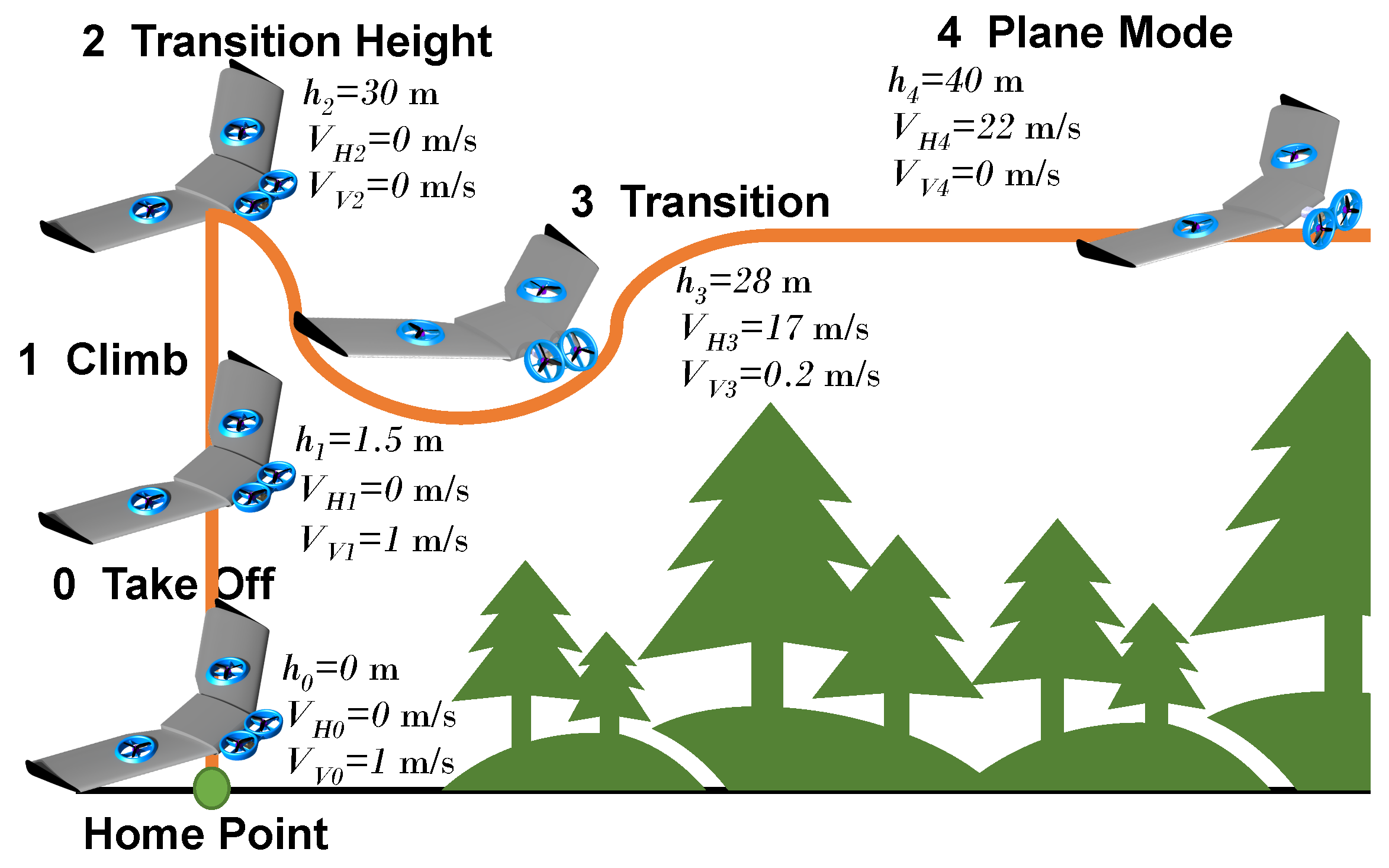
MIL flight simulations were carried out under the atmospheric conditions of Mexico City (see
Table 2). The test consisted of the vehicles taking-off in multirotor flight, climbing until the aircraft reached a transition height defined at 30 m, and then starting the transition phase to plane mode, and once this was completed, maintaining a height of 30 m in straight and level flight. This mission is illustrated in
Figure 15. The same scenario was used to perform a direct comparison between the two VTOL UAV concepts with embedded ducts. By using the same test environment, a fair and accurate evaluation of the performance of both configurations under identical conditions was ensured.
The MIL flight tests were conducted using two computers connected in parallel, one running X-Plane 11.5 and the other one Matlab-Simulink 2022a. The flight tests were carried out with the minimum graphical characteristics, keeping the number of frames per second during the simulation within 30 frames per second (fps), where an interval between 25–35 fps is considered ideal for simulation [
41]. The specifications of the computers used for the development of these simulations were as follows: Laptop ASUS ROG GL752VW with processor Intel Core I7-6700HQ 2.60 GHz, 16 GB RAM, graphics NVIDIA Geforce GTX 960M and Windows 10 Home, and Xtreme PC Gamer AMD Radeon Vega Renoir Ryzen 7 5700G 3.8 GHZ, RAM 16GB, and Windows 10 Pro.
Figure 16,
Figure 17,
Figure 18 and
Figure 19 show the simulation results for height, attitude (pitch and roll), transition signals, energy parameters, and aerodynamic performance using X-Plane and Simulink after simulating each of the vehicles using MIL under the same conditions.
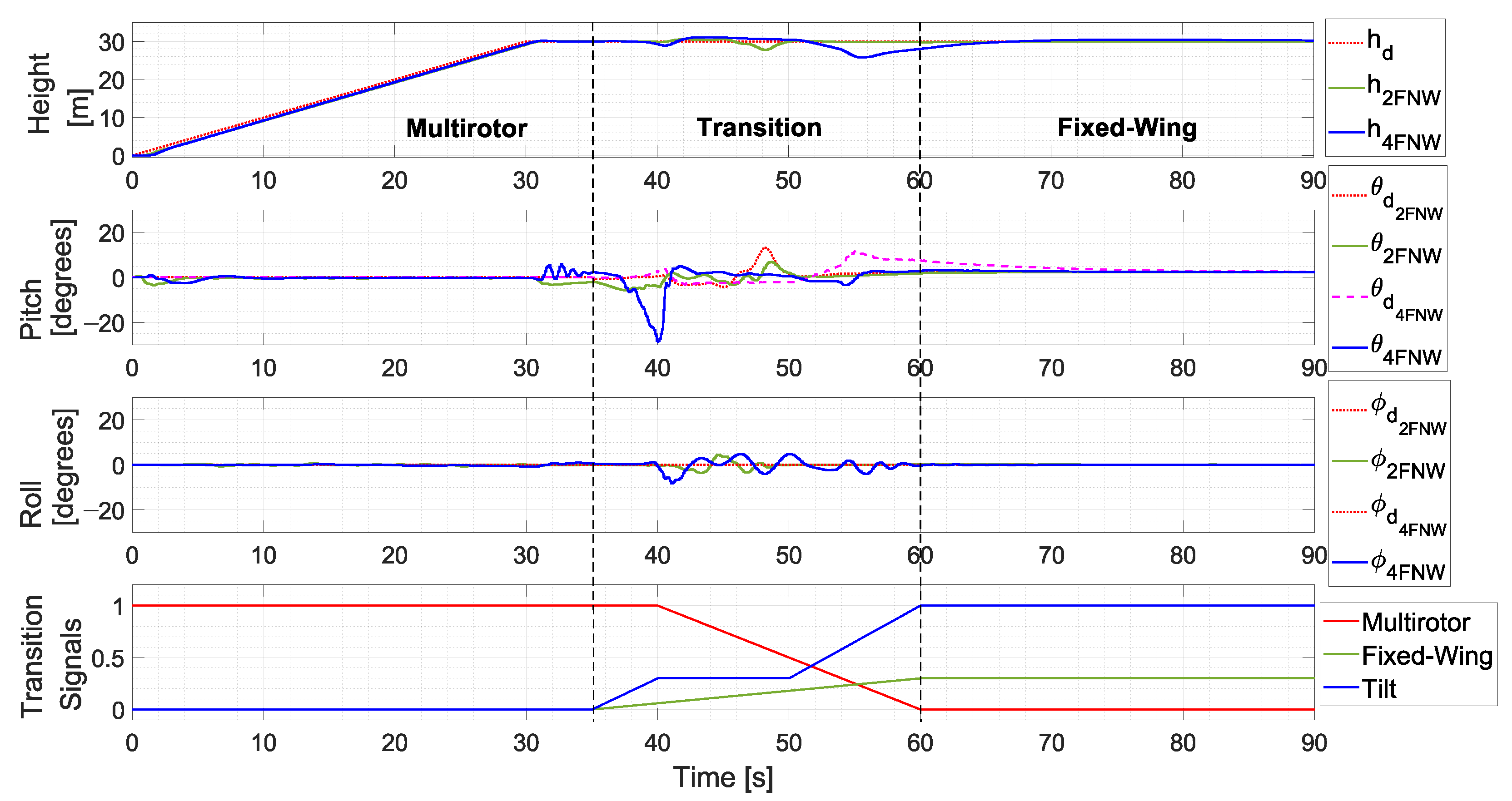
It can be seen from the height plot of the
Figure 16 that the vehicle ascended to a height of 30 m in multirotor flight at a climb velocity of 1 m/s, remaining at this height for 5 s. Then, it began the transition to fixed-wing mode 35 s after taking-off. First, it rotated forward the tilting mechanism in a step-wise manner, while gradually increasing the thrust of its two front engines until it reached 30% of the throttle, in order to gain airspeed. At 40 s, the multirotor mode controller action started to decrease, along with the dedicated ducted fans embedded inside the wing; turning them off avoids pushing air through the duct, eliminating the additional resistance caused by the spinning blades and reducing the total energy consumption and increasing the aircraft’s endurance.
During the transition, the engines were controlled by two systems: the multirotor controller, and the fixed-wing controller. Due to this tilting action, the front engines experienced a decrease in performance related to pitching dynamics, resulting in a noticeable nose-down pitch of the vehicle, as shown in
Figure 16. This nose-down pitch during the transition, as long as it is small, has no influence on the roll dynamics. However, if its magnitude increases, it starts to affect the roll of the vehicle. The transition phase ends at 60 s, when the propulsion reaches its established throttle at 30%, the roll and pitch angles converge to zero degrees, while the vehicle flies level at a height of 30 m.
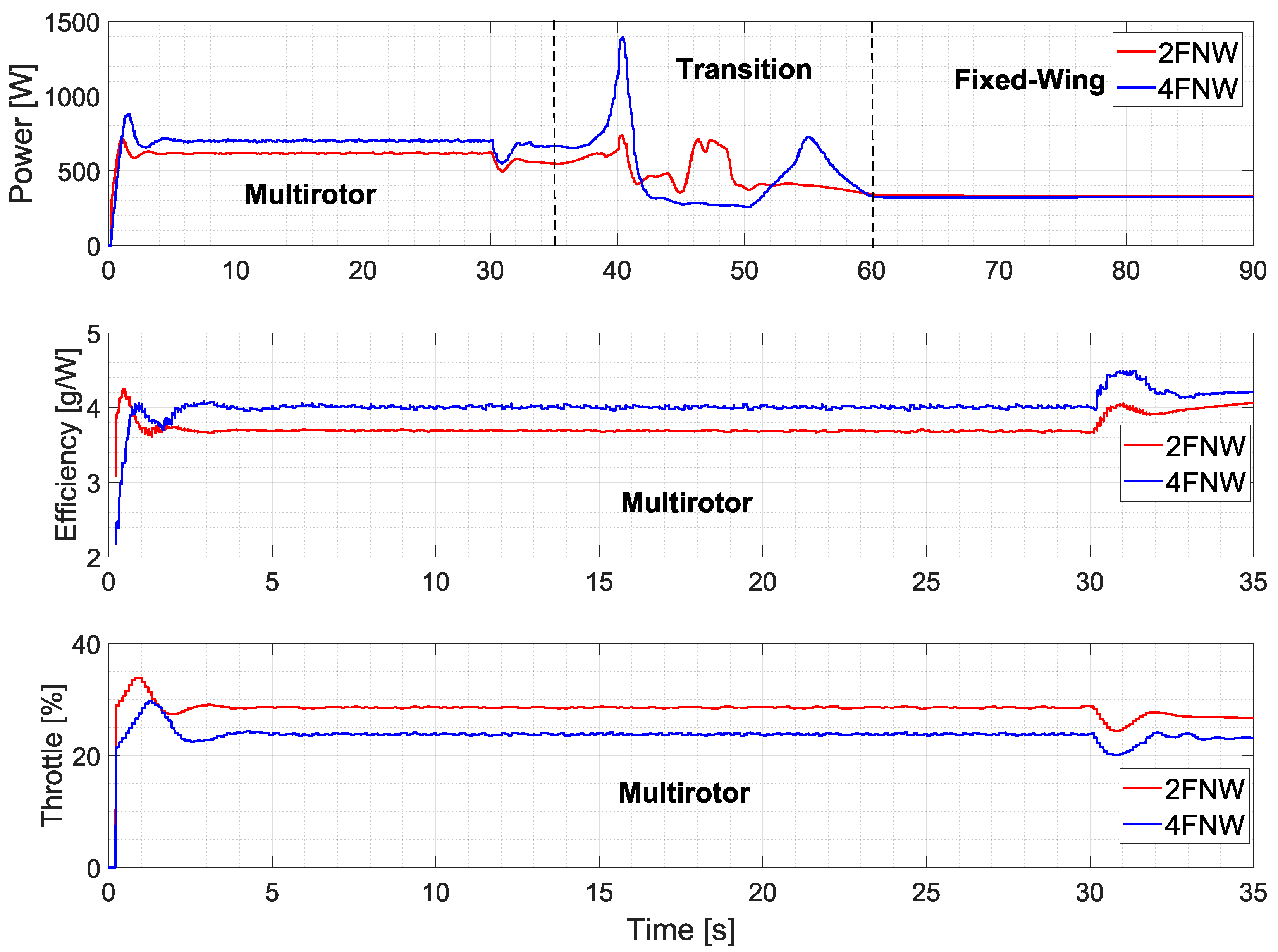
The results depicted in
Figure 17 show three energy parameters obtained during the simulation of the two vehicles. The power graph shows the electrical power consumption of the propulsion system from second 0 to 35 during the multirotor phase. From second 35 to 40, the power consumption increased, since at this point the vehicle was transitioning from the multirotor mode to the fixed-wing mode and it required more energy to compensate for the loss of altitude. After reaching the mark at second 40, a reduction in power consumption became evident. This was attributed to the gradual transition from multicopter mode to fixed-wing mode. In this phase, the aircraft entered into a nose-down dive due to the decrease in thrust generated by the front ducted fans and the insufficient lift to sustain fixed-wing flight mode. At this point, the altitude dynamic was commanded by the control surfaces, while the throttle input was increased until the vehicle reached sufficient airspeed to exclusively use the fixed-wing controller.
In
Figure 17, related to the obtained power results, the beginning and end of the transition phase are indicated by dashed lines at t = 35 s and t = 60 s, respectively. These lines represent the start of the tilting action and its conclusion. Once the transition was finalized, the tilting ducted fans only produced forward thrust, at t = 60 s. We can see that at second 60, there was a significant decrease of 100% in the power consumption during the fixed-wing phase. This reduction can be attributed to the aerodynamic lift generated by the wings, enabling efficient sustained flight. This contrasts with the multirotor mode, where the lift was primarily a result of rotors thrust, demanding a continuous power supply to maintain the vehicle flight.
Analyzing the multirotor phase, the 4FNW platform consumed additional power due to the inclusion of two extra ducted fans, in contrast to the 2FNW, which operated with a lower power demand; however, a closer examination of the energy efficiency graph reveals that the 4FNW reached an energy efficiency of 4 g/W, while for the 2FNW this was 3.6 g/W, proving that the 4FNW was the more energy efficient vehicle. This advantage stems from the distribution of the vehicle’s weight among a greater number of ducted fans, enabling them to function at lower throttle percentages and resulting in a more efficient operation. Looking at the throttle graph, it can also be seen that for the case of vehicles 2FNW and 4FNW, increasing the number of engines lowered the percentage of throttle required.
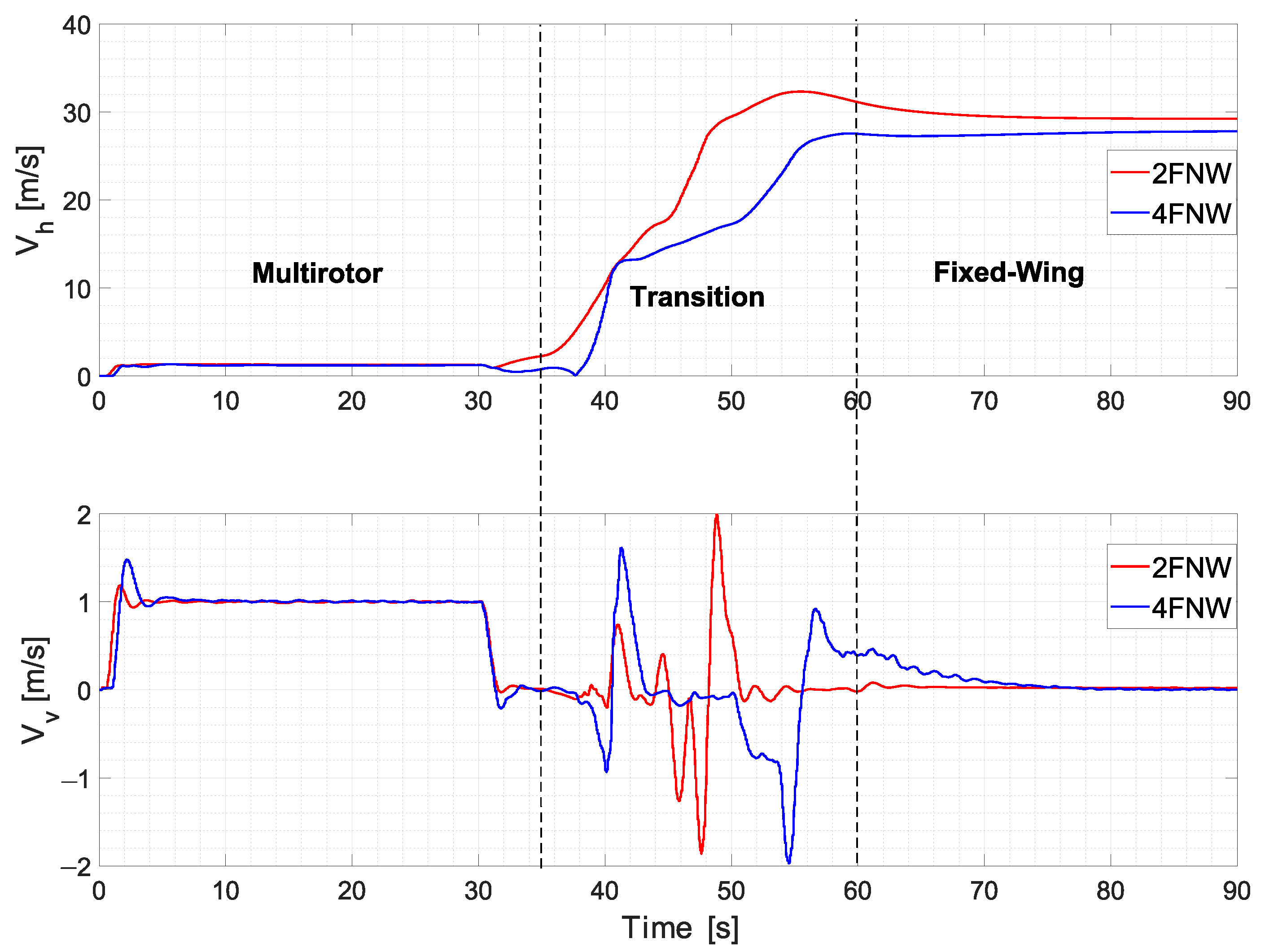
The graph in
Figure 18 shows the airspeed and climb speed. Both platforms were observed to ascend at a constant climb speed of 1 m/s during the multirotor flight. On the other hand, an increase in airspeed can be noticed as both aircraft reached their maximum speeds while flying fixed-wing, employing only 30% of throttle, and achieving an airspeed of 29 and 27 m/s for the 2FNW and 4FNW aircraft, respectively. The 2FNW vehicle, being lighter in weight compared to the 4FNW, achieved a higher airspeed.
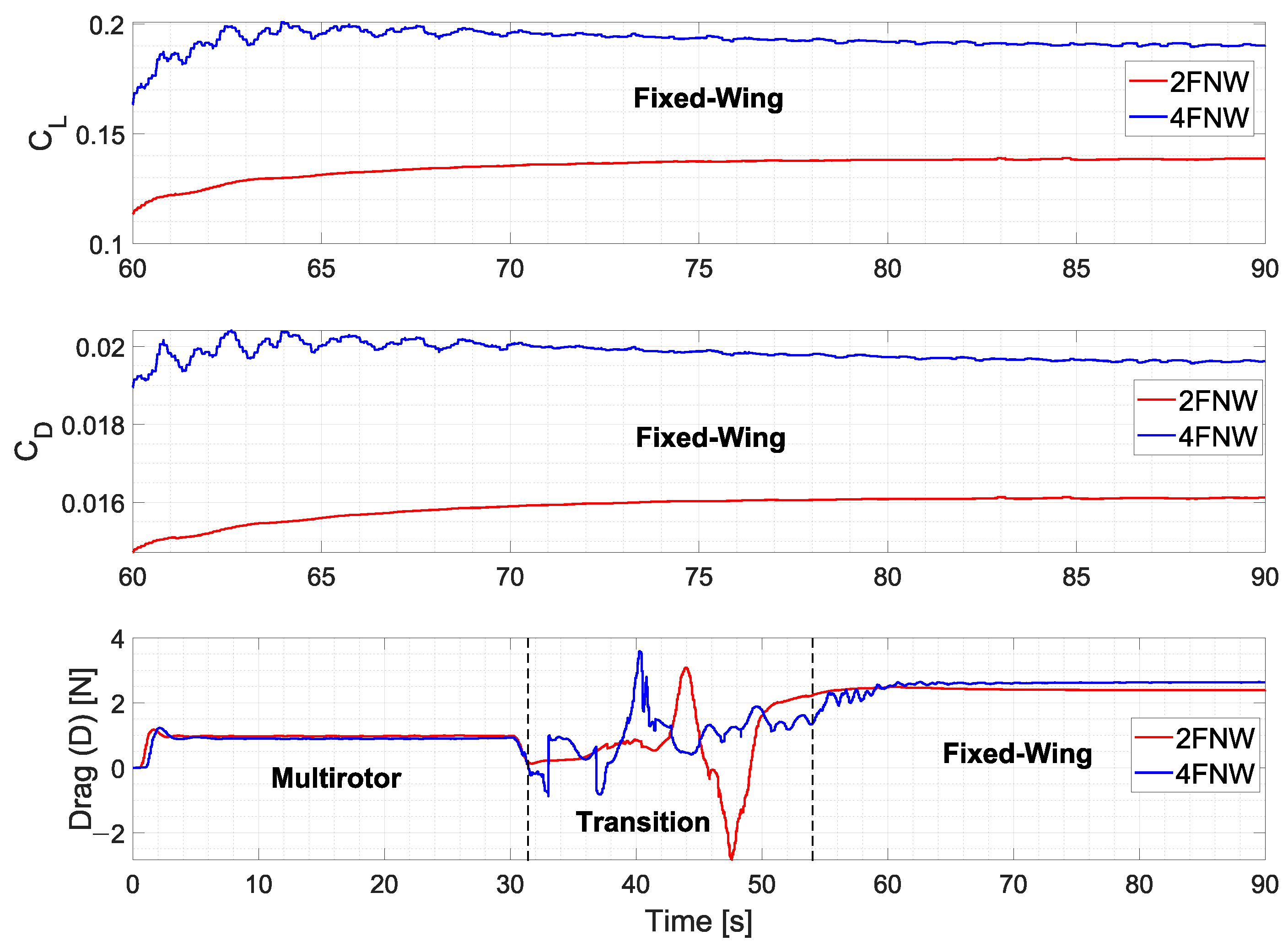
Figure 19 depicts the aerodynamic results obtained during the MIL simulations, and the three graphs correspond to the lift coefficient (
), drag coefficient (
), and the drag force (D).
The coefficient results are presented for the fixed-wing flight mode. It can be observed that, at the start of this phase, there was an increase in due to the vehicles needing to ascend to reach the target altitude. At the beginning of this phase, the vehicles were flying at low airspeed, and the method of compensating for this was raising the angle of attack. This adjustment led to an increase in . However, as the airspeed continued to rise, the coefficient decreased until it stabilized at a constant value. This stabilization indicated that the vehicle had entered a cruising phase. During cruising, the 4FNW was the vehicle with the higher , due to its greater weight compared to the 2FNW, necessitating increased lift.
On the other hand, the exhibited a similar behavior to the , increasing at the beginning due to induced drag, but then decreasing until it reached the minimum value during the cruise phase. This demonstrates the increase in drag for the 4FNW during this stage in comparison to the other aircraft. This can be attributed to the dirtier configuration resulting from the additional ducted fans.
The drag results during the multirotor flight presented a value of approximately 0.9 N, similarly for the two vehicles. Drag is encountered due to the fact that a vehicle generates a force that opposes its vertical displacement. This drag is influenced by factors such as the wing surface area and the rate of climb.
5. Conclusions and Future Work
This research addressed the challenge of improving the energy efficiency of H-VTOL aircraft. To deal with this issue, an innovative aerial vehicle design incorporating a DEP system in conjunction with ducted-fan rotors was proposed. Mathematical models for the XEVTOL-2FNW configuration were developed using the Newton–Euler formalism, enabling the design and implementation of a control strategy for conducting model-in-the-loop simulations in X-Plane. Two configurations were investigated, characterized by a different number of ducted-fan rotors: a four-rotor configuration and a six-rotor configuration. The developed MIL flight simulations enabled the evaluation and analysis of the performance of the proposed propulsion system, showing the following:
An increase of up to 10% in energy consumption for the 4FNW vehicle during the multirotor phase, attributed to the two extra ducted fans consuming more power compared with the 2FNW. However, the 4FNW proved to be 11% more energy efficient on a per rotor basis, as its propulsion system generated more thrust for the same power consumption.
A decrease in electrical power consumption on both platforms when switching from multirotor to the fixed-wing phase, reducing the power consumed by 100%. The power consumed by the 4FNW during the fixed wing phase, increased by only 1% compared with the 2FNW vehicle.
During the fixed-wing phase, the 2FNW vehicle achieved an up to 7.4% higher airspeed compared to the 2FNW vehicle during cruising, attributed to its lighter weight.
The aerodynamic results from the MIL simulation show that both platforms presented a drag force during vertical ascent due to the wing surface, which is in contrast to conventional multirotors, where this force is considered insignificant. Moreover, it was determined that during the fixed-wing flight in cruise condition, the 4FNW produced an increase of up to 46% in the lift coefficient, due to the fact that more lift was required because it is a heavier vehicle. With respect to the vehicle’s drag, the 4FNW produced an increase of up to 19% in the drag coefficient when the vehicle was in cruising flight, due to the extra ducted fans.
In forthcoming research, an analysis of the propulsion system performance will include an analysis of the drag generated by the wing surface during vertical take off, as well as the optimization of the climbing speed during the VTOL phase, in order to reduce the energy consumption due to the extra drag force. Moreover, integrating an altitude controller, through utilizing the pitch angle in conjunction with the thrust to enhance the vehicle’s altitude response during the transition and fixed-wing flight modes, will be considered in the future development of our project. Further certainty regarding the aerodynamic performance of these vehicles could potentially be obtained through additional analyses based on CFD and wind tunnel tests. The study of these XEVTOL concepts using software-in-the-loop and hardware-in-the-loop simulations could provide more information about the performance of these vehicles, to provide feedback for the design process. Similarly, conducting experimental flight tests to validate the numerical results obtained from the simulations will be considered. Finally, in order to improve the performance of the VTOL platforms in the transition phase, the possibility of using the embedded wing ducted fans to generate lift, compensating for the absence of airflow over the wings until the aircraft reaches the desired airspeed, will be evaluated.


 ,
, 


