Waypoint Generation in Satellite Images Based on a CNN for Outdoor UGV Navigation

Abstract

Moving on paths or trails present in natural environments makes autonomous navigation of unmanned ground vehicles (UGV) simpler and safer. In this sense, aerial photographs provide a lot of information of wide areas that can be employed to detect paths for UGV usage. This paper proposes the extraction of paths from a geo-referenced satellite image centered at the current UGV position. Its pixels are individually classified as being part of a path or not using a convolutional neural network (CNN) which has been trained using synthetic data. Then, successive distant waypoints inside the detected paths are generated to achieve a given goal. This processing has been successfully tested on the Andabata mobile robot, which follows the list of waypoints in a reactive way based on a three-dimensional (3D) light detection and ranging (LiDAR) sensor.

1. Introduction

With more information available in the environment, path-planning methods for an unmanned ground vehicle (UGV) can generate better results [1]. For off-road navigation, especially in uneven terrain, it is helpful to use a digital elevation map to avoid non-traversable zones for UGVs [2,3].

Long-range navigation of UGVs requires not only processing of onboard sensor data but also requires taking advantage of prior environmental knowledge provided by overhead data [4]. This is particularly convenient for less structured outdoors such as disaster areas [5], natural terrains [6], and agricultural fields [7].

On natural terrains, it is common to find footpaths employed by persons or animals that connect different places of interest. If present, they can be employed by UGVs to facilitate their movements because they usually represent the safer ways in such environments. These trails can be followed by an UGV [8] or an unmanned aerial vehicle (UAV) [9] to facilitate and to speed up autonomous navigation.

Images acquired from satellites provide a lot of information on wide areas that can be employed to detect paths for UGV usage [10]. Moreover, UAVs can collaborate with UGVs to acquire aerial photographs on site [11,12,13].

Semantic segmentation of aerial images represents a classic machine vision problem [14], which can be solved with supervised [15] and deep learning, mainly with convolutional neural networks (CNNs) [16,17,18,19]. For urban areas, the output classes of the CNN usually includes roads, buildings, cars, and trees [20].

Reliable CNN training requires a lot of images labelled pixel by pixel as input, which can be available in public datasets [21,22]. Synthetic data are a relevant alternative for training both traditional machine [23] and deep learning methods [24] because ground truth data can be labelled automatically, which avoids tedious and error-prone manual or assisted tagging [25].

In this paper, it is proposed to extract paths from satellite imagery to facilitate UGV navigation on outdoors. Its main contribution comes from the combination of the following procedures:

• A CNN has been trained with automatically labelled synthetic data to extract possible paths on natural terrain from a satellite image.
• Geo-referenced waypoints along the detected path from the current UGV location are directly generated from the binarised image.

Figure 1 shows a general scheme of the proposed method. Once the satellite image is captured from Google maps, its pixels are classified and geo-referenced. Then, a search algorithm is used to calculate a list of distant waypoints that an UGV can follow.

This processing has been applied for outdoor navigation of the mobile robot Andabata, using a three-dimensional (3D) light detection and ranging (LiDAR) sensor to follow reactively the generated waypoints.

The rest of the paper is organized as follows. The next section describes satellite image segmentation using a CNN which has been trained with synthetic data. Then, waypoint generation from the binarised image is described in Section 3. Section 4 presents the results of applying the proposed method. Finally, the paper ends with the conclusions and the references.

2. Image Segmentation

In this section, the generation of synthetic aerial images with the robotic simulation tool Gazebo is described first. Then, it is shown how these data can be automatically labelled and employed for training a CNN for path detection. Finally, validation results are presented with synthetic and real data.

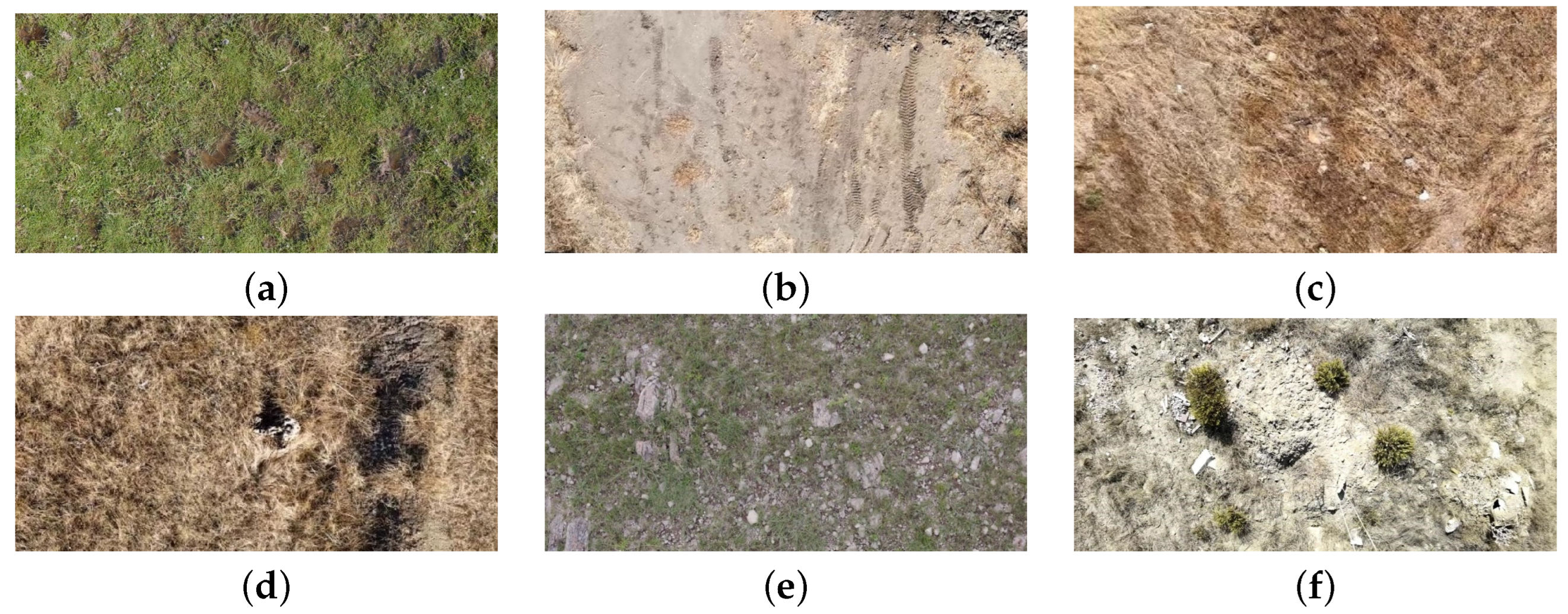
2.1. Natural Environment Modelling

Gazebo is an open-source 3D robotics simulator with integrated physics engine [26] that allows the development of realistic models of complex environments [25]. In this way, it has been used as a simulation environment for technological challenges [27].

The first step to model a natural environment with Gazebo is to build a two-dimensional (2D) map that contains the variable-width paths. There is no need for elevation maps for this purpose because it is assumed that images will be captured at sufficient height.

The map consists of a square with 300 $\mathrm{m}$ side and a resolution of 27,000 × 27,000 pixels. The terrain and path surfaces have been generated separately with the graphics software Blender v3.3 LTS (https://www.blender.org, accessed on 20 June 2023). The terrain surface contains gaps that exactly match the path surface (see Figure 2).

In addition, textures from real images have been employed to cover the terrain surface and mimic the visual aspect of natural environments. Figure 3 shows the textures used, which include diverse vegetation in sandy and rocky terrains. Similarly, three different textures can cover the surface of the paths (see Figure 4).

All these textures have been composed in terrain and path patchworks with the same square dimensions of the 2D map (see Figure 5). Then, these patchworks are stuck to their corresponding surfaces in Gazebo.

Additionally, several trees have been incorporated directly to the virtual environment (see Figure 6). These are the unique elements with height that can produce shadows. The final aspect of the modelled natural environment can be observed in Figure 7.

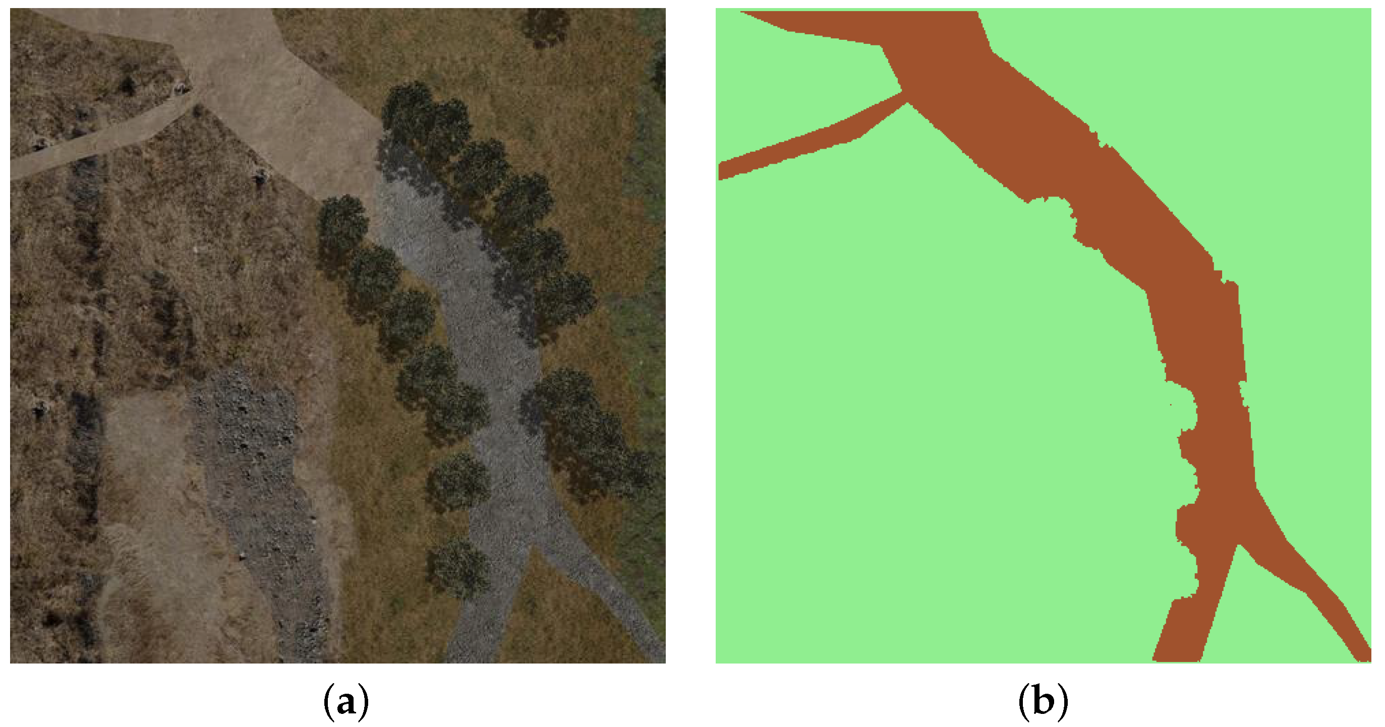
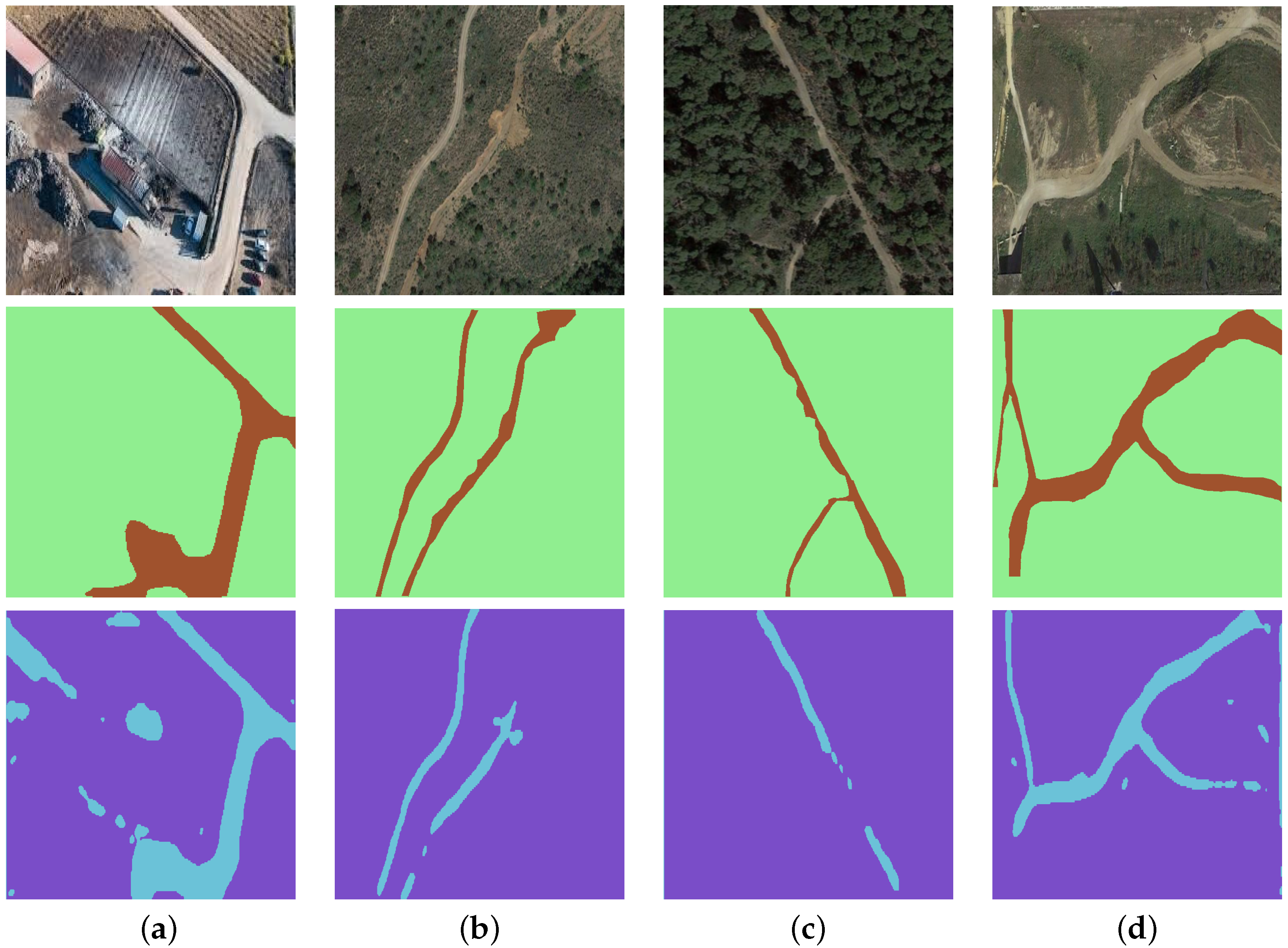
2.2. Annotated Aerial Images

A duplicate of the synthetic environment is used to obtain annotated images with its pixels classified into the path and non-path categories in red and green colours, respectively (see Figure 8). In the duplicate, textures have been replaced by flat colours and trees have been included into the non-path class. This map is very similar to the one shown in Figure 2, but it is not exactly the same.

The open-source Robot Operating System (ROS) [28] has been integrated into Gazebo [29] to acquire aerial images of the environment and record them on bag files. Concretely, photographs are obtained by simulating the camera provided by Gazebo with a resolution of 480 × 480 pixels.

The camera is placed 60 $\mathrm{m}$ above the map on spots so that no borders appears in the images. Two different photographs are acquired from the same location, one from the realistic environment and the other from the two-colour version, having both images an exact correspondence of pixels.

Figure 9 illustrates the image generation procedure with synthetic aerial photographs that corresponds to a given camera location above the map. All in all, 567 pairs of images (realistic and labelled) have been generated for training, and 115 pairs for validation. The classes are unbalanced: the majority of pixels of the annotated images belongs to the non-path class (87.7%) and the rest (12.3%) to the path class.

2.3. The ResNet-50 CNN

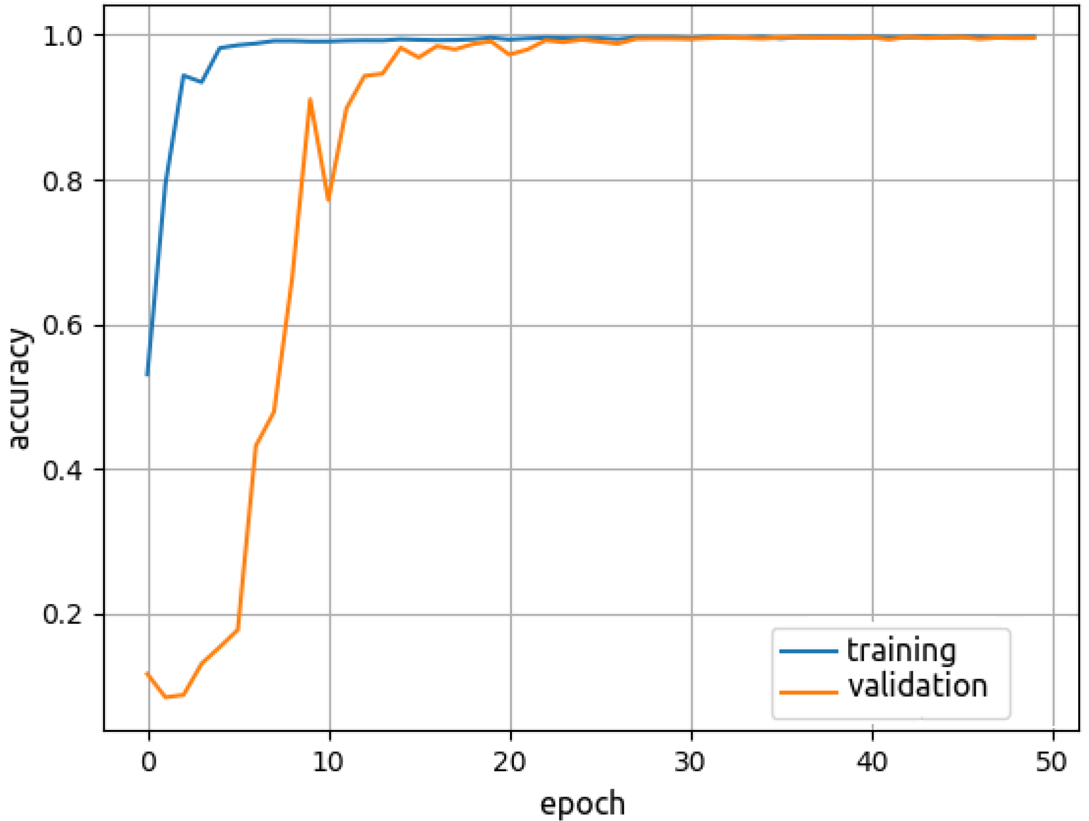
A CNN is a type of neural network architecture commonly used in computer vision tasks [30]. These networks implement in at least one of its layers a mathematical operation called convolution that serves to extract relevant features.

A ResNet (RESidual Neural NETwork) is the CNN chosen for path detection. It is characterized by adding residual shortcuts through the network for gradient propagation during training to avoid accuracy degradation [31]. The TensorFlow v2.9 library (https://www.tensorflow.org, accessed on 20 June 2023) [32], together with the Python interface provided by Keras [33,34], have been employed for developing the ResNet.

Figure 10 shows the ResNet structure implemented in Keras (https://github.com/divamgupta/image-segmentation-keras, accessed on 20 June 2023) for path detection with 50 different layers, which includes convolutional, identity (ID), pooling, rectification (RELU), batch normalization, flattening and fully connected blocks. The residual shortcuts are inside the blocks of the three stages shown in Figure 10. The input and output images of this ResNet have always a size of 480 × 480 pixels.

Resnet has been trained using 47 epochs and 10 steps per epoch. The selected CNN at the 27 epoch achieves an overall accuracy of 0.98 and avoids overfitting both in the training and validation data (see Figure 11).

2.4. Validation

Four segmentation examples of synthetic images from the validation data are shown in Figure 12, where purple and cyan colours represent the obtained non-path and path classes, respectively.

Table 1. Components of the confusion matrices for synthetic and real validation data.

Component	Synthetic Data	Real Data
True Positive (TP)	105,141	64,608
True Negative (TN)	800,324	813,920
False Positive (FP)	2434	18,497
False Negative (FN)	13,701	24,575

contains the components of the confusion matrix for the synthetic validation data of Figure 12 by considering negative and positive the non-path and path classes, respectively.

The CNN has been also applied to satellite images of natural environments using web mapping services. Satellite images are obtained through the Google maps API (https://developers.google.com/maps/documentation/maps-static, accessed on 20 June 2023) using a zoom level of 19 that adjusts a square of 143 $\mathrm{m}$ side with 640 × 640 pixels. These images are first rescaled to the size employed by ResNet-50 (480 × 480 pixels).

The four examples shown in Figure 13 have been manually labelled. In the first case, it can be observed that the CNN classifies the roof of a farm and part of the sown field as a path. In the others, there are path segments that are not detected. The components of the confusion matrix for these real data can be found in Table 1.

Performance metrics have been computed in

Table 2. Validation metrics in synthetic and real data for path detection with ResNet-50.

Metric	Formula	Synthetic Data	Real Data
Precision	$\frac{TP+TN}{TP+TN+FP+FN}$	0.9824	0.9533
Recall (RE)	$\frac{TP}{TP+FN}$	0.8847	0.7244
Specificity (SP)	$\frac{TN}{TN+FP}$	0.9969	0.9778
Balanced Accuracy	$\frac{RE+SP}{2}$	0.9408	0.8511

for both synthetic and real data, where good classification results can be observed. Although the obtained accuracy with real data is slightly worse than with synthetic data, the main paths remain well highlighted in these examples.

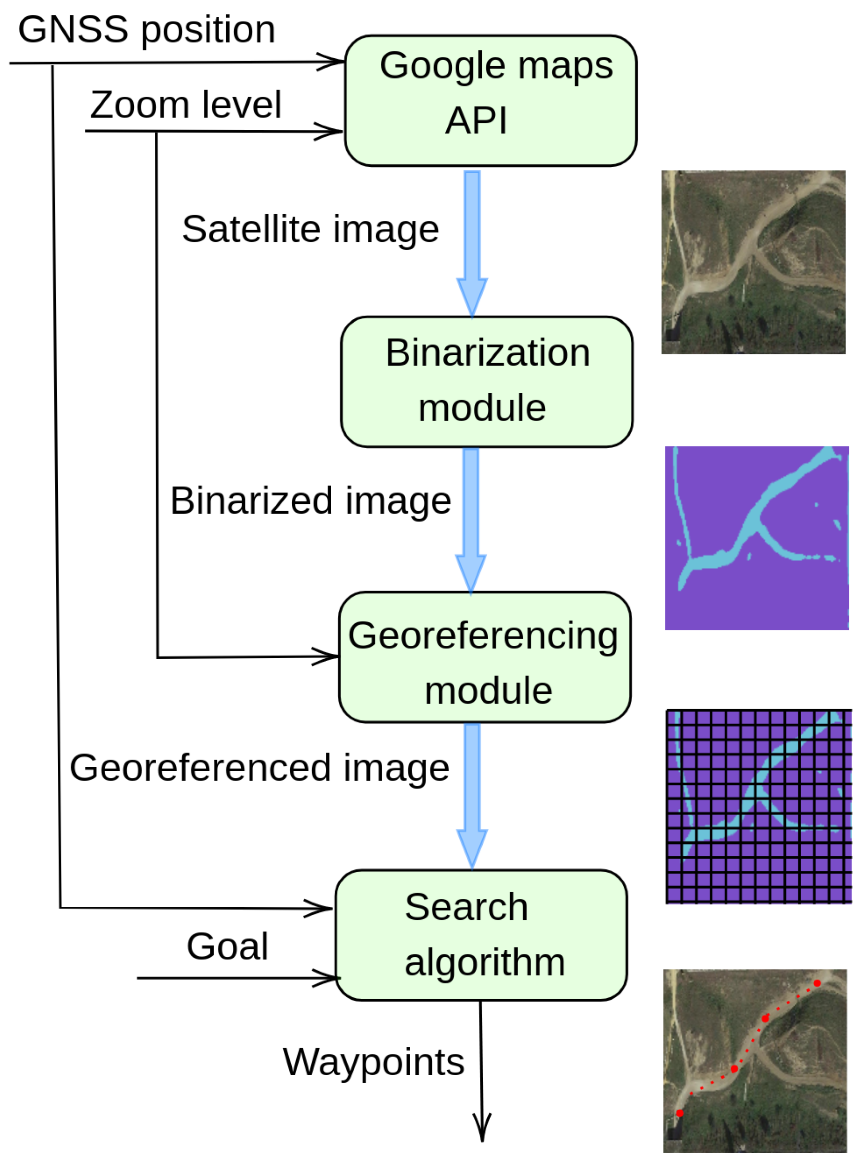
3. Waypoint Generation

In this section, the binarised pixels of the image are geo-referenced. Then, a search algorithm is applied to generate an ordered list of waypoints towards a goal. Lastly, a graphical user interface (GUI) for waypoint visualization is presented.

3.1. Pixel Geo-Referencing

Each pixel from a satellite image obtained through the Google maps API centred at the current UGV geodetic position need to be geo-referenced. Google Maps tiles employs a universal transverse Mercator (UTM) to assign coordinates to locations on the surface of the Earth, ignoring their altitude.

Binarised images are firstly rescaled to the original size (640 × 640 pixels). For a given latitude in degrees, the meters per pixel factor can be calculated as:

$$K_{pix}=\frac{cos(2\times \pi \times R\times \frac{latitude\times \pi }{180})}{256\times zoom},$$

(1)

where $zoom=19$ is the selected map zoom and $R$ = 6,378,137 m is the radius of the Earth.

Figure 14 shows the reference systems needed to assign UTM coordinates to every pixel in the image. The centre of the image correspond to the current UGV position, with the X and Y axes pointing to the east and to the north, respectively. Let u and v be the number of pixels from the upper-left corner of the image in the X and Y directions, respectively.

Given the UTM coordinates of the centre of the image (north $N_0$ and east $E_0$ obtained from the longitude and latitude coordinates of the UGV), it is possible to calculate the UTM coordinate of each pixel as:

$$E=E_0+(u-320)\times K_{pix},N=N_0+(320-v)\times K_{pix},$$

(2)

where 320 represents half of the image side.

3.2. Pixel Route

A standard A* algorithm [35] has been used to calculate a pixel route along the detected path on the binarised image. The search is performed by connecting the pixels that correspond to the centre of the image with the user-defined goal, assuming that both fall inside the same path.

The output of the A* algorithm is a list of adjacent pixels. Waypoints are chosen every 70 pixels (approximately with a separation of 18 $\mathrm{m}$). Finally, their corresponding UTM positions for UGV navigation can be obtained with (2).

3.3. Developed GUI

A GUI has been programmed in order to indicate the goal of the UGV and to supervise the whole process. The following buttons are available:

• “Get Map” to obtain a satellite view centred on the current UGV position.
• “Binarise” to segment the image using the trained CNN.
• “Global Plan” to calculate waypoints to the selected goal.
• “Toggle View” to alternate between the satellite view and the binarized one.
• “Quit” to abandon the application.

Figure 15 displays the appearance of the programmed interface. The cursor can be employed to indicate the desired goal on the segmented image. It can be observed the UGV location marked with a green dot and the available user buttons at the right.

4. Experimental Results

In this section, the proposed method is checked on an intricate satellite image. Then, it is tested for outdoor navigation of a mobile robot in an urban park.

4.1. Generating Waypoints

Figure 16 shows a satellite photograph where multiple paths are visible. Most of the paths have been detected well in the segmented image, including the one where the UGV is located.

The pixel routes calculated by A* in opposite directions along the UGV path are shown with red lines in Figure 17. It can be observed that they remain inside the inner part of the curves. The chosen waypoints are indicated with red dots. These waypoints are generated with a similar separation from the starting position with the exception of the distance between the goal and the last waypoint that may be less.

The following times have been obtained on a computer with an Intel Core i7-9700 processor with eight cores at $3.6$ $\mathrm{G}$$\mathrm{Hz}$: $0.9$ $\mathrm{s}$ for obtaining the image and 4 $\mathrm{s}$ for segmentation. For generating the more complex and simpler pixel routes, it lasts $8.6$ $\mathrm{s}$ and 6 $\mathrm{s}$, respectively.

4.2. Outdoor Navigation

The mobile robot Andabata consists of a wheeled skid-steer vehicle for outdoor navigation (see Figure 18). This battery-operated UGV is $0.67$ $\mathrm{m}$ long, $0.54$ $\mathrm{m}$ wide, $0.81$ $\mathrm{m}$ in height, and weighs 41 $\mathrm{k}$$\mathrm{g}$. The local coordinate frame is placed at the centre of the wheel contact points with the ground, with its local $X_p$, $Y_p$, and $Z_p$ axes pointing forward, to the left and upwards, respectively.

The computer of Andabata employs an inertial measurement unit (IMU), with inclinometers, gyroscopes, and a compass, and a global navigation satellite system (GNSS) receiver with a horizontal resolution of 1 $\mathrm{m}$ included in its onboard smartphone for outdoor localization [36]. The main exteroceptive sensor for navigation is a custom 3D LiDAR sensor with 360 ${}^{\circ }$ field of view built by rotating a 2D LiDAR [37].

Although waypoints for the UGV are calculated in the detected paths, reactivity is still necessary to avoid steep slopes and unexpected obstacles that are not visible on satellite images. Local navigation between distant waypoints has been implemented on Andabata with a previously developed actor–critic scheme, which was trained using reinforcement and curriculum learning [36].

Basically, acquired 3D point clouds are employed to emulate a 2D traversability scanner, which produces 32 virtual levelled ranges up to 10 $\mathrm{m}$ around the vehicle (see Figure 19). These data, together with the heading error of the vehicle with respect to the current waypoint ($p_t$), are employed by the actor neural network to directly produce steering speed commands while moving at a constant longitudinal speed [36]. When the distance to the current waypoint ($d_t$) is less than 1 $\mathrm{m}$, the next objective from the list is chosen.

Figure 20 shows the five waypoints calculated from the binarised satellite image with Andabata in an urban park. It can also be observed in this figure that streets and highways above and below the park, respectively, are not detected as footpaths by the trained CNN.

Two navigation experiments were performed to track the generated waypoints starting from the same position. In the first one, there were no unexpected obstacles. In the second experiment, the UGV meets with two pedestrians at the beginning and at the end.

The paths followed by Andabata with a longitudinal speed of $0.55$ $\mathrm{m}$/$\mathrm{s}$, as obtained by its GNSS receiver, are shown in Figure 21. In total, the UGV travelled $76.2$ $\mathrm{m}$ and 78 $\mathrm{m}$ during 142 $\mathrm{s}$ and 147 $\mathrm{s}$, in the first and second cases, respectively.

Smooth heading changes and a sharp turn at the end of the first trajectory can be observed in Figure 22. Additional heading changes are visible at the beginning and at the end of the second trajectory. Figure 23 contains different views of the detected path from the point of view of the mobile robot.

5. Conclusions

It is common to find footpaths on natural terrains that connect different places of interest. These trails can be detected from aerial images and employed by UGVs to facilitate their displacements.

The paper has presented a method for generating a list of waypoints from satellite images for outdoor UGV navigation. The image is first binarized into two classes according to the belonging of each pixel to a path or not using a CNN, which has been trained using synthetic data automatically labelled with Gazebo and ROS. The binarized image is then geo-referenced, and waypoints are calculated on the detected path between the current UGV position and a user-defined goal.

The implemented ResNet has achieved high accuracy with synthetic data and good results with real satellite data obtained from Google Maps tiles. Moreover, the proposed procedure has been successfully tested on the mobile robot Andabata. For this purpose, it was necessary to integrate waypoint tracking with reactive navigation based on its onboard 3D LiDAR to avoid steep slopes and unexpected obstacles.

Future work includes connecting together possible discontinuous segments of a detected path. It is also of interest to complement satellite data with images from the UGV camera to increase reliability in trail finding.

References

1. Sánchez-Ibáñez, J.R.; Pérez-del Pulgar, C.J.; García-Cerezo, A. Path Planning for Autonomous Mobile Robots: A Review. Sensors 2021, 21, 7898. [Google Scholar] [CrossRef]
2. Hua, C.; Niu, R.; Yu, B.; Zheng, X.; Bai, R.; Zhang, S. A Global Path Planning Method for Unmanned Ground Vehicles in Off-Road Environments Based on Mobility Prediction. Machines 2022, 10, 375. [Google Scholar] [CrossRef]
3. Toscano-Moreno, M.; Mandow, A.; Martínez, M.A.; García-Cerezo, A. DEM-AIA: Asymmetric inclination-aware trajectory planner for off-road vehicles with digital elevation models. Eng. Appl. Artif. Intell. 2023, 121, 105976. [Google Scholar] [CrossRef]
4. Vandapel, N.; Donamukkala, R.R.; Hebert, M. Unmanned Ground Vehicle Navigation Using Aerial Ladar Data. Int. J. Robot. Res. 2006, 25, 31–51. [Google Scholar] [CrossRef] [Green Version]
5. Delmerico, J.; Mueggler, E.; Nitsch, J.; Scaramuzza, D. Active Autonomous Aerial Exploration for Ground Robot Path Planning. IEEE Robot. Autom. Lett. 2017, 2, 664–671. [Google Scholar] [CrossRef] [Green Version]
6. Silver, D.; Sofman, B.; Vandapel, N.; Bagnell, J.A.; Stentz, A. Experimental Analysis of Overhead Data Processing To Support Long Range Navigation. In Proceedings of the IEEE/RSJ International Conference on Intelligent Robots and Systems, Beijing, China, 9–15 October 2006; pp. 2443–2450. [Google Scholar] [CrossRef] [Green Version]
7. Bodur, M.; Mehrolhassani, M. Satellite Images-Based Obstacle Recognition and Trajectory Generation for Agricultural Vehicles. Int. J. Adv. Robot. Syst. 2015, 12, 188. [Google Scholar] [CrossRef]
8. Thrun, S.; Montemerlo, M.; Dahlkamp, H.; Stavens, D.; Aron, A.; Diebel, J.; Fong, P.; Gale, J.; Halpenny, M.; Hoffmann, G.; et al. Stanley: The robot that won the DARPA Grand Challenge. J. Field Robot. 2006, 23, 661–692. [Google Scholar] [CrossRef]
9. Giusti, A.; Guzzi, J.; Ciresan, D.; He, F.L.; Rodriguez, J.; Fontana, F.; Faessler, M.; Forster, C.; Schmidhuber, J.; Caro, G.; et al. A Machine Learning Approach to Visual Perception of Forest Trails for Mobile Robots. IEEE Robot. Autom. Lett. 2016, 1, 661–667. [Google Scholar] [CrossRef] [Green Version]
10. Santos, L.C.; Aguiar, A.S.; Santos, F.N.; Valente, A.; Petry, M. Occupancy Grid and Topological Maps Extraction from Satellite Images for Path Planning in Agricultural Robots. Robotics 2020, 9, 77. [Google Scholar] [CrossRef]
11. Christie, G.; Shoemaker, A.; Kochersberger, K.; Tokekar, P.; McLean, L.; Leonessa, A. Radiation search operations using scene understanding with autonomous UAV and UGV. J. Field Robot. 2017, 34, 1450–1468. [Google Scholar] [CrossRef] [Green Version]
12. Meiling, W.; Huachao, Y.; Guoqiang, F.; Yi, Y.; Yafeng, L.; Tong, L. UAV-aided Large-scale Map Building and Road Extraction for UGV. In Proceedings of the IEEE 7th Annual International Conference on CYBER Technology in Automation, Control, and Intelligent Systems, (CYBER), Honolulu, HI, USA, 31 July–4 August 2018; pp. 1208–1213. [Google Scholar] [CrossRef]
13. Peterson, J.; Chaudhry, H.; Abdelatty, K.; Bird, J.; Kochersberger, K. Online Aerial Terrain Mapping for Ground Robot Navigation. Sensors 2018, 18, 630. [Google Scholar] [CrossRef] [PubMed] [Green Version]
14. Montoya-Zegarra, J.A.; Wegner, J.D.; Ladický, L.; Schindler, K. Semantic Segmentation of Aerial Images in Urban Areas with Class-Specific Higher-Order Cliques. ISPRS Ann. Photogramm. Remote Sens. Spat. Inf. Sci. 2015, II-3/W4, 127–133. [Google Scholar] [CrossRef] [Green Version]
15. Wang, M.; Chu, A.; Bush, L.; Williams, B. Active detection of drivable surfaces in support of robotic disaster relief missions. In Proceedings of the IEEE Aerospace Conference, Big Sky, MT, USA, 2–9 March 2013. [Google Scholar] [CrossRef]
16. Hudjakov, R.; Tamre, M. Aerial imagery terrain classification for long-range autonomous navigation. In Proceedings of the International Symposium on Optomechatronic Technologies (ISOT), Istanbul, Turkey, 21–23 September 2009; pp. 88–91. [Google Scholar] [CrossRef]
17. Krizhevsky, A.; Sutskever, I.; Hinton, G.E. ImageNet Classification with Deep Convolutional Neural Networks. In Advances in Neural Information Processing Systems; Pereira, F., Burges, C., Bottou, L., Weinberger, K., Eds.; Curran Associates, Inc.: Red Hook, NY, USA, 2012; Volume 25. [Google Scholar]
18. Sermanet, P.; Eigen, D.; Zhang, X.; Mathieu, M.; Fergus, R.; LeCun, Y. Overfeat: Integrated recognition, localization and detection using convolutional networks. In Proceedings of the 2nd International Conference on Learning Representations (ICLR), Banff, AB, Canada, 14–16 April 2014. [Google Scholar]
19. Delmerico, J.; Giusti, A.; Mueggler, E.; Gambardella, L.M.; Scaramuzza, D. “On-the-Spot Training” for Terrain Classification in Autonomous Air-Ground Collaborative Teams. In Proceedings of the 2016 International Symposium on Experimental Robotics, Nagasaki, Japan, 3–8 October 2016; Kulić, D., Nakamura, Y., Khatib, O., Venture, G., Eds.; Springer: Berlin/Heidelberg, Germany, 2017; pp. 574–585. [Google Scholar] [CrossRef]
20. Ding, L.; Tang, H.; Bruzzone, L. LANet: Local Attention Embedding to Improve the Semantic Segmentation of Remote Sensing Images. IEEE Trans. Geosci. Remote Sens. 2021, 59, 426–435. [Google Scholar] [CrossRef]
21. Máttyus, G.; Luo, W.; Urtasun, R. DeepRoadMapper: Extracting Road Topology from Aerial Images. In Proceedings of the IEEE International Conference on Computer Vision (ICCV), Venice, Italy, 22–29 October 2017; pp. 3458–3466. [Google Scholar] [CrossRef]
22. Chen, K.; Fu, K.; Yan, M.; Gao, X.; Sun, X.; Wei, X. Semantic Segmentation of Aerial Images With Shuffling Convolutional Neural Networks. IEEE Geosci. Remote Sens. Lett. 2018, 15, 173–177. [Google Scholar] [CrossRef]
23. Martínez, J.L.; Morán, M.; Morales, J.; Robles, A.; Sánchez, M. Supervised Learning of Natural-Terrain Traversability with Synthetic 3D Laser Scans. Appl. Sci. 2020, 10, 1140. [Google Scholar] [CrossRef] [Green Version]
24. Nikolenko, S. Synthetic Simulated Environments. In Synthetic Data for Deep Learning; Springer Optimization and Its Applications; Springer: Berlin/Heidelberg, Germany, 2021; Volume 174, Chapter 7; pp. 195–215. [Google Scholar] [CrossRef]
25. Sánchez, M.; Morales, J.; Martínez, J.L.; Fernández-Lozano, J.J.; García-Cerezo, A. Automatically Annotated Dataset of a Ground Mobile Robot in Natural Environments via Gazebo Simulations. Sensors 2022, 22, 5599. [Google Scholar] [CrossRef] [PubMed]
26. Koenig, K.; Howard, A. Design and Use Paradigms for Gazebo, an Open-Source Multi-Robot Simulator. In Proceedings of the IEEE-RSJ International Conference on Intelligent Robots and Systems, Sendai, Japan, 28 September–2 October 2004; pp. 2149–2154. [Google Scholar] [CrossRef] [Green Version]
27. Agüero, C.E.; Koenig, N.; Chen, I.; Boyer, H.; Peters, S.; Hsu, J.; Gerkey, B.; Paepcke, S.; Rivero, J.L.; Manzo, J.; et al. Inside the Virtual Robotics Challenge: Simulating Real-Time Robotic Disaster Response. IEEE Trans. Autom. Sci. Eng. 2015, 12, 494–506. [Google Scholar] [CrossRef]
28. Quigley, M.; Conley, K.; Gerkey, B.; Faust, J.; Foote, T.; Leibs, J.; Wheeler, R.; Ng, A. ROS: An open-source Robot Operating System. In Proceedings of the IEEE ICRA Workshop on Open Source Software, Kobe, Japan, 12 May 2009; Volume 3, pp. 1–6. [Google Scholar]
29. Bechtsis, D.; Moisiadis, V.; Tsolakis, N.; Vlachos, D.; Bochtis, D. Unmanned Ground Vehicles in Precision Farming Services: An Integrated Emulation Modelling Approach. In Information and Communication Technologies in Modern Agricultural Development; Springer: Berlin/Heidelberg, Germany, 2019; Volume 953, pp. 177–190. [Google Scholar] [CrossRef]
30. Murphy, K.P. Probabilistic Machine Learning: An Introduction; MIT Press: Cambridge, MA, USA, 2022. [Google Scholar]
31. He, K.; Zhang, X.; Ren, S.; Sun, J. Deep Residual Learning for Image Recognition. In Proceedings of the IEEE Conference on Computer Vision and Pattern Recognition (CVPR), Las Vegas, NV, USA, 27–30 June 2016; pp. 770–778. [Google Scholar] [CrossRef] [Green Version]
32. Abadi, M.; Agarwal, A.; Barham, P.; Brevdo, E.; Chen, Z.; Citro, C.; Corrado, G.S.; Davis, A.; Dean, J.; Devin, M.; et al. TensorFlow: Large-Scale Machine Learning on Heterogeneous Systems. In Proceedings of the 12th USENIX Symposium on Operating Systems Design and Implementation (OSDI), Savannah, GA, USA, 2–4 November 2016. [Google Scholar]
33. Gulli, A.; Pal, S. Deep Learning with Keras; Packt Publishing Ltd.: Birmingham, UK, 2017. [Google Scholar]
34. Gupta, D. A Beginner’s Guide to Deep Learning Based Semantic Segmentation Using Keras. 2019. Available online: https://divamgupta.com/image-segmentation/2019/06/06/deep-learning-semantic-segmentation-keras.html (accessed on 20 June 2023).
35. Foead, D.; Ghifari, A.; Kusuma, M.; Hanafiah, N.; Gunawan, E. A Systematic Literature Review of A* Pathfinding. Procedia Comput. Sci. 2021, 179, 507–514. [Google Scholar] [CrossRef]
36. Sánchez, M.; Morales, J.; Martínez, J.L. Reinforcement and Curriculum Learning for Off-Road Navigation of an UGV with a 3D LiDAR. Sensors 2023, 23, 3239. [Google Scholar] [CrossRef] [PubMed]
37. Martínez, J.L.; Morales, J.; Reina, A.; Mandow, A.; Pequeño Boter, A.; García-Cerezo, A. Construction and calibration of a low-cost 3D laser scanner with 360o field of view for mobile robots. In Proceedings of the IEEE International Conference on Industrial Technology (ICIT), Seville, Spain, 17–19 March 2015; pp. 149–154. [Google Scholar] [CrossRef]
Figure 1. Overview of the processing pipeline. Calculated waypoints on the detected path are indicated with red dots.
Machines 11 00807 g001
Figure 2. Terrain and path surfaces on the map represented in dark and light grey, respectively.
Machines 11 00807 g002
Figure 3. Terrain textures: green high grass (a), loose sand (b), dry grass (c), dry bushes (d), rocky terrain with grass (e) and hard sand with sparse bushes (f).
Machines 11 00807 g003
Figure 4. Path textures: reddish (a), brownish (b), and greyish (c).
Machines 11 00807 g004
Figure 5. Texture patchworks for the terrain (a) and the paths (b).
Machines 11 00807 g005
Figure 6. The 3D Gazebo models of trees included in the environment.
Machines 11 00807 g006
Figure 7. Realistic model of a natural environment.
Machines 11 00807 g007
Figure 8. Flat colour map of the natural terrain in Gazebo.
Machines 11 00807 g008
Figure 9. Synthetic aerial images with realistic (a) and flat (b) colours.
Machines 11 00807 g009
Figure 10. The implemented ResNet-50 structure.
Machines 11 00807 g010
Figure 11. Accuracy evaluation of ResNet-50 during training and with validation data.
Machines 11 00807 g011
Figure 12. Semantic segmentation on four synthetic validation examples (ad): realistic (top), labelled (middle) and classified (bottom) images.
Machines 11 00807 g012
Figure 13. Real (top), manually labelled (middle), and CNN-segmented (bottom) images from a farmland (a), mountain pathway (b), forest trail (c) and urban park (d).
Machines 11 00807 g013
Figure 14. Coordinate systems for the geo-referenced image.
Machines 11 00807 g014
Figure 15. Aspect of the developed GUI.
Machines 11 00807 g015
Figure 16. Satellite image with multiple visible paths (a) and segmentation result (b). The green dot at the center indicates the UGV location.
Machines 11 00807 g016
Figure 17. Waypoints generated in opposite path directions (a,c) and visualization on the satellite image (b,d). Pixel route is indicated with a red line and waypoints with red dots.
Machines 11 00807 g017
Figure 18. The mobile robot Andabata.
Machines 11 00807 g018
Figure 19. Representation of a virtual 2D traversability scan for Andabata [36]. A nearby obstacle is shown in grey.
Machines 11 00807 g019
Figure 20. Waypoints generated on the park environment on the binarized (a) and satellite images (b).
Machines 11 00807 g020
Figure 21. First and second paths followed by Andabata (red and blue lines, respectively) and calculated waypoints (black circles). The initial position of the mobile robot is marked with an X.
Machines 11 00807 g021
Figure 22. Heading of Andabata during the first and second experiments marked with red and blue lines, respectively.
Machines 11 00807 g022
Figure 23. Park views along the tracked path from the camera of the onboard smartphone.
Machines 11 00807 g023