1. Introduction
Vehicle suspension systems play a pivotal role in enhancing the comfort, driving safety, and handling stability of vehicles [
1,
2,
3]. In comparison to conventional steel plate springs, air springs offer notable advantages such as superior vibration isolation, cost-effectiveness, broad applicability, and convenient adjustability. Consequently, an increasing number of commercial vehicles are adopting air suspension system structures [
4,
5,
6]. Furthermore, with the advancements in vehicle networking technology, researchers now have easy access to extensive real-world vehicle driving data. Leveraging this operational data for evaluating or designing vehicle parameters can yield more optimal design solutions [
7,
8]. Hence, it is imperative to investigate and assess air suspension systems using operational data derived from vehicle networks.
Numerous scholars have extensively researched the optimization and design of air suspension systems [
9,
10,
11,
12,
13,
14]. However, several concerns regarding the design of air suspension systems for passenger vehicles remain unresolved. Firstly, most existing studies assume fixed suspension system parameters during the design process. However, the vibration isolation performance of the suspension system is adversely affected by the fluctuating sprung mass of the bus, which is contingent upon the number of passengers. This inconsistency leads to unstable performance. Secondly, only a limited number of studies have accounted for fluctuations in suspension system parameters [
15,
16]. These studies assume probability distributions based on empirical knowledge, but the inherent errors between the assumed and true probability distributions are evident.
Consequently, this study aims to resolve the issue of unstable vibration isolation performance caused by fluctuating sprung mass in the air suspension system. To achieve this, the sprung mass is treated as a random input, and the probability distribution range of the performance response of the system is analyzed. Moreover, to ensure the accuracy of the sprung mass probability distribution, a deep neural network (DNN) model is trained using experimental data for sprung mass identification. Using vehicle network data, the DNN model accurately identifies the sprung mass of a bus during operation and determines its true probability distribution.
Vehicle parameters are commonly assumed to be deterministic, but they can undergo variations due to design, manufacturing, assembly, and usage conditions [
17,
18]. For instance, the difference between the full and unladen mass of a bus can account for 40–50% of the vehicle’s total mass. These significant mass fluctuations profoundly impact the performance of suspension systems, necessitating the quantification of the influence of uncertain mass on suspension system performance variations [
19]. Various uncertainty propagation methods have been proposed in other domains. Nagy and Braatz categorized these methods into analytical, sampling, and response surface-based approaches [
20]. The analytical method, although highly efficient, requires knowledge of the explicit expression of the response function [
21]. The Monte Carlo method offers the highest accuracy [
22], but it demands a large number of samples and becomes computationally intensive when dealing with complex response calculation models. The response surface method trains the response function using input–output pairs from the computational model, but it also incurs significant computational costs during the training process [
23]. To address the computational burden associated with uncertainty analysis of suspension system performance, Xu et al. applied the polynomial chaos expansion method to evaluate the uncertainty response of the quarter air suspension system performance, thereby enhancing the analysis efficiency of the air suspension system [
15].
Uncertainty parameters are typically assumed to follow standard probability distributions, such as the normal distribution or exponential distribution. These distributions provide readily available random numbers that adhere to their specific properties [
24]. In this study, actual operational data is utilized to determine the mass, resulting in probability distribution functions that often deviate from standard types of distributions. To ensure the accuracy of the sprung mass probability distribution during uncertainty analysis, direct sampling of non-standard probability density functions is necessary. The accept-reject sampling method is capable of sampling arbitrary probability density functions [
25]. Hence, this paper incorporates the accept–reject sampling method in the uncertainty analysis of bus air suspension systems.
To accurately determine the probability density function of the sprung mass, it is imperative to identify the entire vehicle mass of an operational bus. Numerous approaches have been proposed by scholars for vehicle mass identification, depending on specific research requirements [
26,
27]. Initially, researchers incorporated additional sensors to gather suspension dynamic deflection data and then calculated the sprung mass using a suspension dynamics model [
28,
29]. Vahidi et al. proposed recursive least squares with forgetting factors to identify mass and slope under diverse road conditions [
30]. Sun et al. combined recursive least squares with a Kalman filter to identify road slope and mass for city buses [
31]. Zhang et al. utilized a two-layer reinforced estimator for mass and road-slope estimation of electric mining vehicles [
32]. This paper does not adopt these methods, as it lacks the dynamic deflection data required by the suspension dynamic deflection approach and aims to employ existing vehicle network data for mass identification. Recursive methods are prone to cumulative estimation errors, resulting in inaccurate estimates. Machine learning techniques are adept at mitigating cumulative estimation errors and can yield more precise outcomes when a large number of data are available. Consequently, this study intends to employ deep neural networks to estimate the overall vehicle mass of city buses. The main contributions of this paper can be summarized as follows:
- (1)
A data-driven process is proposed in this study for analyzing the uncertainties in an air suspension system. By utilizing vehicle data from the internet, a deep neural network model is employed to accurately identify the sprung mass of city buses and determine its probability distribution characteristics. Subsequently, the uncertainty analysis of the performance of the bus air suspension system is conducted using the rejection sampling method.
- (2)
The impact of the sprung mass and its varying probability distributions on the uncertain response of suspension system performance is analyzed. Both sinusoidal and broadband excitations are considered.
The remainder of this paper is structured as follows:
Section 2 establishes the dynamic model of the bus air suspension system.
Section 3 employs a deep neural network for the identification of the sprung mass. In
Section 4, we conduct an uncertainty analysis of the air suspension system using the rejection sampling algorithm. Finally,
Section 5 provides the conclusion.
3. Data-Driven Statistical Analysis of Sprung Mass
The aim of this section is to develop a quantitative model for uncertainty in the mass of a bus. In the uncertainty analysis and optimal design of air suspension systems, the probability distributions of the uncertainty parameters are usually used in a hypothetical way [
15,
16]. Obviously, there is bound to be some deviation between the assumed probability distribution and the actual probability distribution, which will lead to the uncertainty analysis results deviating from the real situation.
In order to solve the above problem, this section identifies the real mass data through operational data and performs statistical analysis to obtain an accurate probability distribution of sprung mass. The main steps are: establishing the longitudinal dynamics equations of the bus, which are used to determine the type of data to be collected; identifying sprung mass using DNN; and establishing statistically the probability distribution pattern of the sprung mass.
3.1. DNN-Based Bus Mass Identification
3.1.1. Feature Parameter Selection and Data Pre-Processing
We determined the chosen characteristic parameters based on the equations for the longitudinal dynamics of the bus.
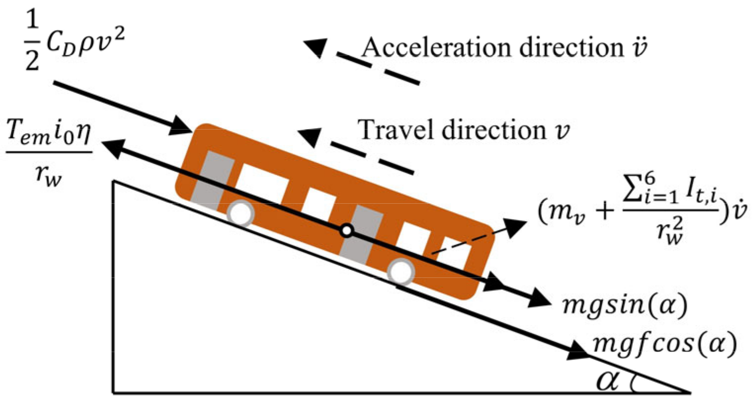
Figure 5 shows the forces on the body of a purely electric bus while driving. The longitudinal dynamics equation can be expressed as
where
Fi is the inertial force,
Fa is the aerodynamic force,
Fr is the rolling resistance,
Fg is the gravitational force,
Fp is the propulsion, and
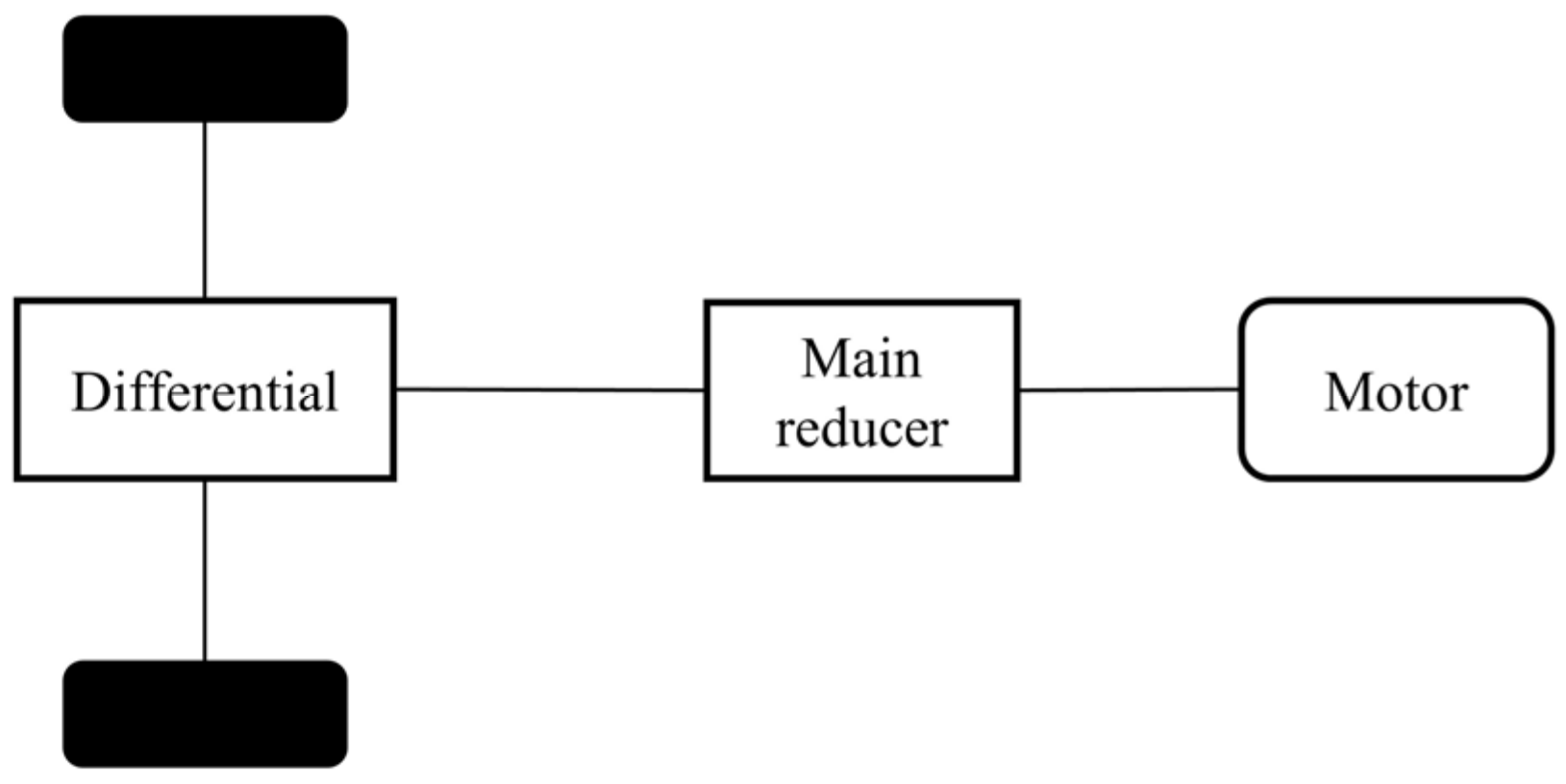
Fe is the system error. Based on automotive theory and the air suspension system configuration of the pure electric bus in
Figure 6, the expression for each force in Equation (13) can be derived as
mv is the overall vehicle mass,
It is the equivalent rotational inertia of the wheels,
rt is the tyre rolling radius,
v is the vehicle speed,
CD is the air resistance coefficient,
A is the windward area,
ρ is the air density,
g is the acceleration of gravity,
f is the rolling resistance coefficient,
α is the road gradient,
Tem is the motor torque,
i0 is the main gearbox speed ratio, and
η is the mechanical efficiency, and is taken as 0.9.
According to Equation (14), the vehicle mass and the road gradient are coupled. To achieve vehicle mass recognition, the road gradient needs to be estimated at the same time. The road gradient is related to the acceleration measured by the accelerometer, as follows, and the vehicle travel acceleration, the road gradient and the acceleration measured by the accelerometer are related as follows:
where
asensor is the acceleration signal measured by the accelerometer. Considering Equations (13) and (15) together, some vehicle design parameters are fixed and can be gradually adapted during the training of the neural network, whereas
v,
,
Tem and
asensor are variable in real time, in line with the driving process, and need to be handled separately.
Referring to [
35],
v,
,
Tem and
asensor are critical to the recognition accuracy of the mass. When the vehicle parameters are fixed, the value of the air resistance term depends on the vehicle speed; the magnitude of acceleration resistance depends on the acceleration; the motor torque, as the sole power source, determines the driving state of the vehicle; and the longitudinal acceleration sensor collected by the accelerometer can decouple the road slope and mass. So,
v,
,
Tem and
asensor are chosen as feature parameters.
The longitudinal acceleration can be obtained by differentiation of the velocity, so only the velocity signal and the time signal need to be acquired. In addition, when the driver brakes, there is a possibility of mechanical braking force, which is difficult to obtain accurately. In order to avoid the influence of the data during braking on the estimation results, it is necessary to exclude the periods when the braking force is not 0. The braking force can be judged according to whether the brake pedal signal Tbrake is 0 or not. In summary, the signals to be acquired are the moment, vehicle speed, motor torque, accelerometer signal and brake pedal signal.
The data collected are of different types and scales, and differ by several orders of magnitude. To avoid the calculation results being influenced by large values, the data collected are normalized using the z-score normalization method.
3.1.2. DNN Structure
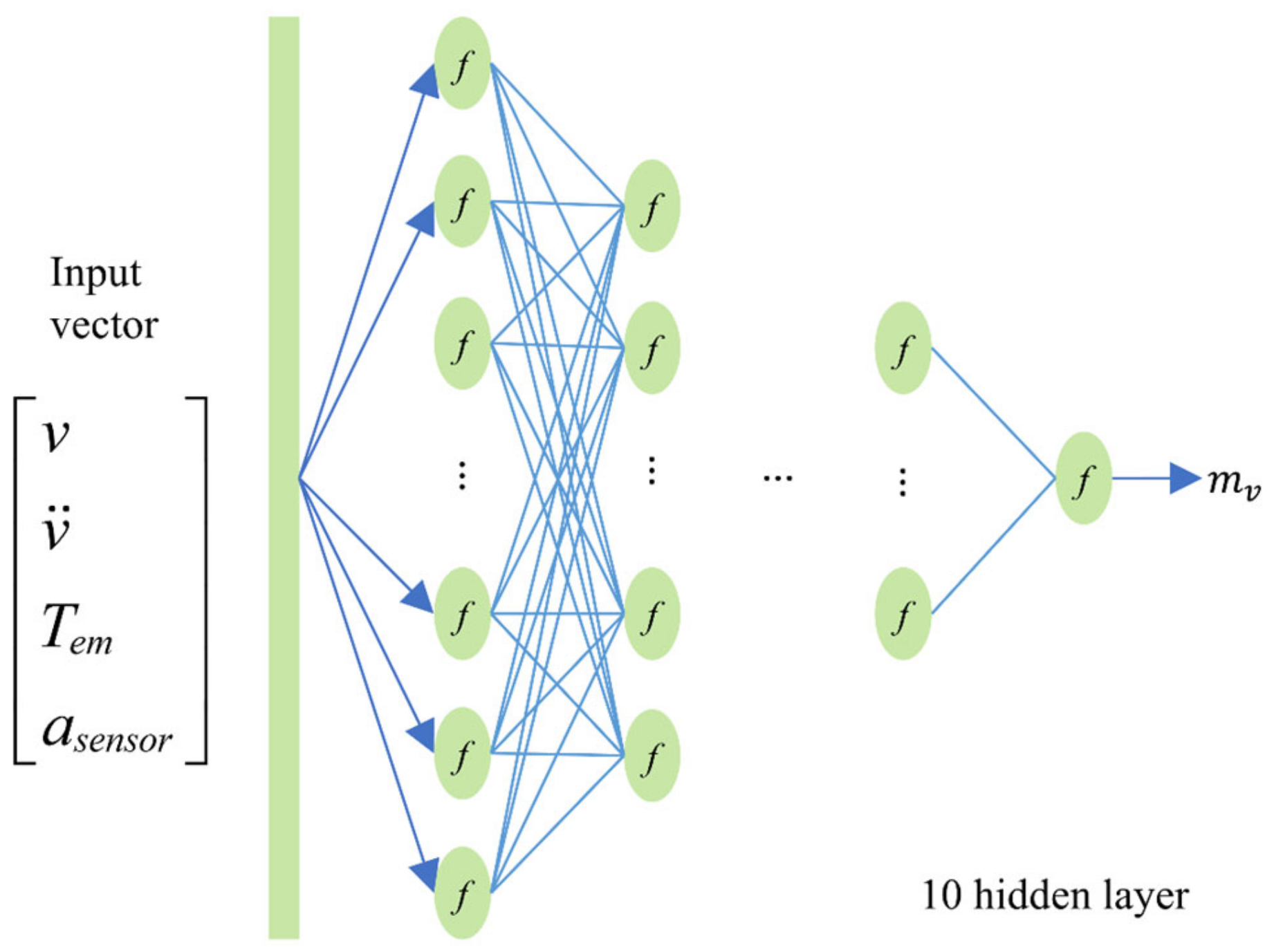
In order to estimate the mass of the whole vehicle, we considered a neural network with 10 hidden layers, the number of neurons in each layer being 100, 90, …, 10, 1, the output of each neuron being the input of the neuron in the next layer.
Figure 7 shows the structure of the DNN. When training the DNN, we chose the Leaky rectified linear unit function as the activation function
In addition, to prevent overfitting, regularization methods are usually used, and we choose the computationally efficient L2 regularization method. In this way, after setting the hidden layers, the number of neurons, the activation function and the regularization method, the feature parameters and quality labels are input into the DNN, and the weights and biases in the network are continuously optimized, resulting in a DNN that can be used for quality estimation.
3.1.3. Model Training and Validation
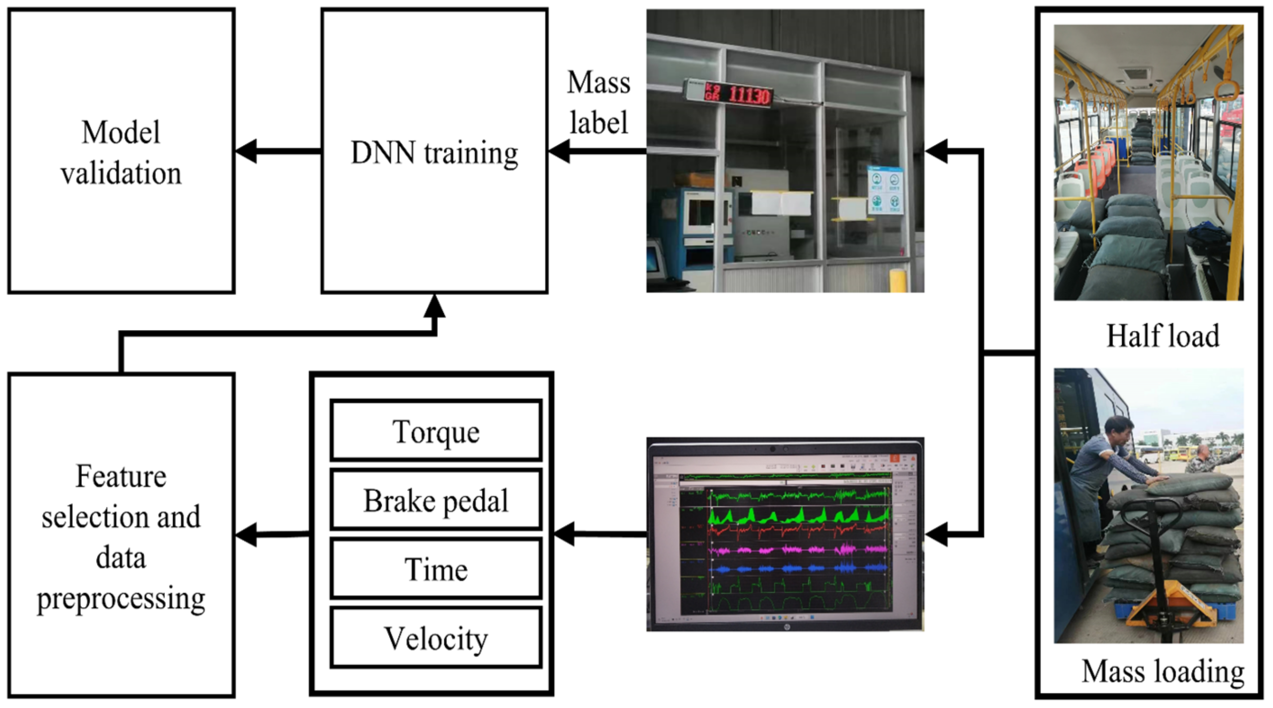
In order to validate the effectiveness of the proposed mass identification method, we carried out relevant experiments on a bus test track.
Figure 8 shows the experimental equipment and the process of validating the mass estimation model: (1) loading mass with sand bags; (2) obtaining mass labels through a weighbridge; (3) simulating the actual driving process of the bus; (4) using the on-board intelligent terminal to obtain the controller area network (CAN) Bus in
v,
Tem,
Tbrake and
asensor; and (5) training the DNN model in MATLAB.
A total of 15 experiments of different quality were carried out, and 80% of each data set was selected as the training set, with the remaining 20% as the validation set.
We used DNN and RLS (recursive least squares) [
30] to identify vehicle mass. The respective recognition results are shown in
Table 2. The DNN has a maximum average relative error of 5.3%, while RLS has a maximum average relative error of 6.2%. Additionally, RLS also exhibits larger errors in other aspects. These results indicate that the proposed trained DNN network method has a better recognition accuracy than RLS.
The disparity stems from the dependence of RLS on vehicle parameters, including f, CD, , and others. Regrettably, these parameters frequently lack the precision required for accurate mass identification, as factors like vehicle speed and load introduce variability, notably affecting f. This limitation hampers RLS’s effectiveness in achieving precise mass identification outcomes. Conversely, DNN transcends the necessity for exact vehicle parameters. With sufficient data, DNN can iteratively converge towards accurate values, enabling progressively refined recognition results.
3.2. Bus Mass Identification and Statistical Analysis
A bus factory’s vehicle networking platform stores most of its own vehicle driving data on a server via the internet, which provides a large amount of basic data for statistical analysis of bus mass. Therefore, we can directly download the historical operating data of the buses from the telematics system, pre-process the data, and then identify the quality of the buses.
Due to the network environment, there was a problem of missing data in the telematics data, and it was difficult to fill in the missing data for a long period of time, so we could only choose to eliminate the motion segments with missing data. The quality of the telematics data was affected by the performance of the terminal equipment, and the resolution of the data was low, only 1 Hz, while the quality recognition algorithm required a resolution of 10 Hz for the input data, so linear interpolation needed to be chosen to improve its resolution.
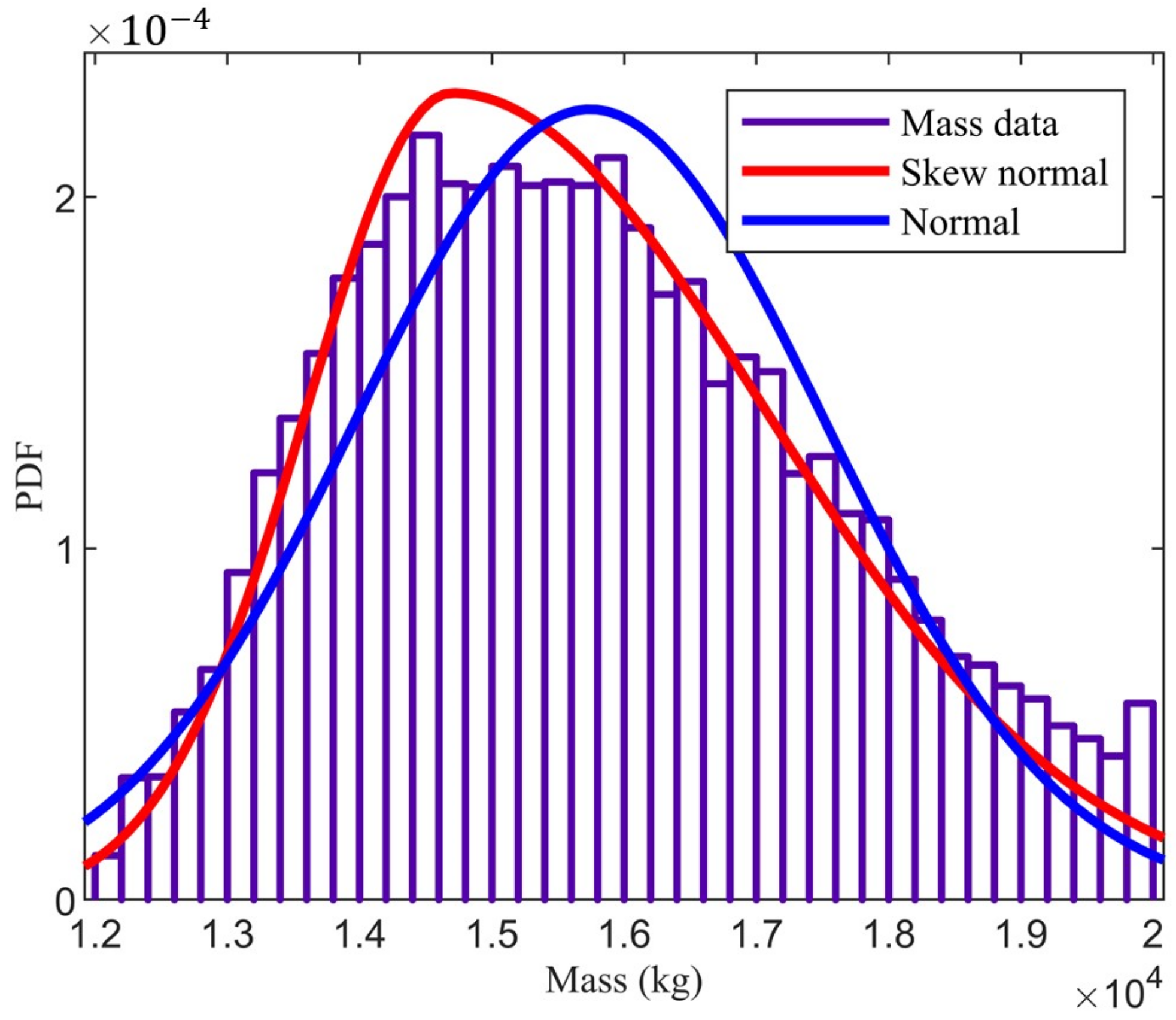
The vehicle networking data was downloaded through the bus telematics platform for 50 days of operation. To ensure that the trained DNN network could be used for the bus, the design parameters of the bus needed to be consistent with the test bus. The data types were time, vehicle speed, motor torque and brake pedal signals. Invalid driving segments were removed, linear interpolation was used to improve the data resolution, and the trained DNN was used to identify the vehicle mass to obtain 50 days of mass data for this vehicle. After statistical analysis, the mean value was 15,742 and the standard deviation was 1773.
The frequency distribution histogram is shown in
Figure 9. It can be seen from the graph that the mass distribution does not conform to the standard normal distribution, and the data distribution is skewed to the left of the mean. The probability density functions of the masses are fitted with the normal and skewed normal distributions respectively, and their respective fitted curves are also plotted in
Figure 9. It can be found that the skewed probability density curves in the rising and falling phases of the probability density function (PDF) curve fit the true masses more closely, so we chose the skew normal distribution fitting method. The distribution parameters are location value of 14,696, scale value of 1737, and skewness value of −0.3667.
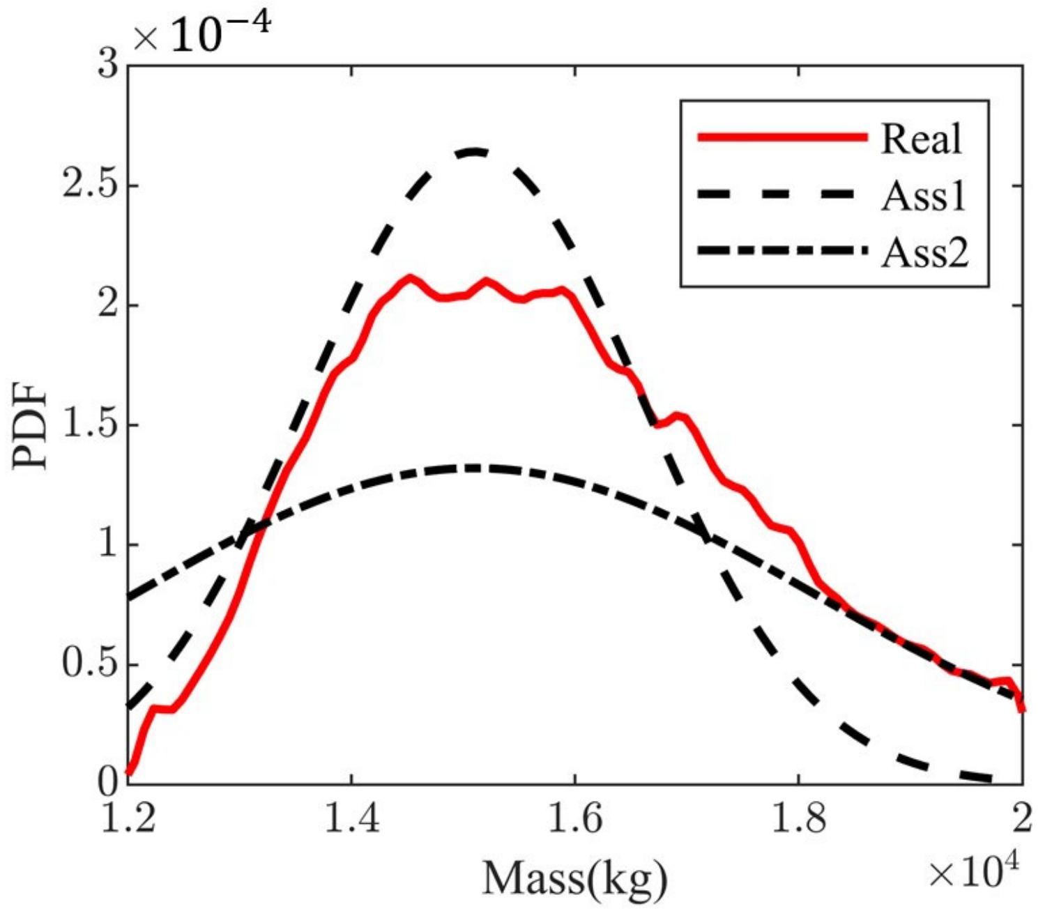
Reference [
15] expresses the uncertainty of air suspension system parameters as a normal distribution containing different coefficients of variation, i.e., a standard deviation of 0.1 or 0.2 times the mean value. We compared the probability density based on the coefficients of variation with the probability density of the true statistics in this paper, as shown in
Figure 10. In
Figure 10, Ass1 and Ass2 denote probability density curves with coefficients of variation of 0.1 and 0.2, and Real denotes the PDF curve of the real statistics. It can be found that Ass1 is larger than Real near the peak, while Ass2 is smaller than Real; both Ass1 and Ass2 are larger than Real in the rising phase; and both Ass1 and Ass2 are smaller than Real in the falling phase. In general, the PDF based on the coefficient of variation is very different to the PDF of the real statistics.
Table 3 compares the mean and standard deviation of masses under different statistical approaches. The mean value of Real is larger than that of Ass because of overloading during the actual operation and a higher probability density over a large mass range. The standard deviation of Real is between the two Asses, indicating that the mass distribution of Ass1 is too concentrated, while the estimated mass distribution of Ass2 is too loose.
4. Data-Driven Uncertainty Analysis of Bus Air Suspension Systems
The whole vehicle dynamics model in
Section 2 and the statistical results of the whole vehicle mass probability distribution in
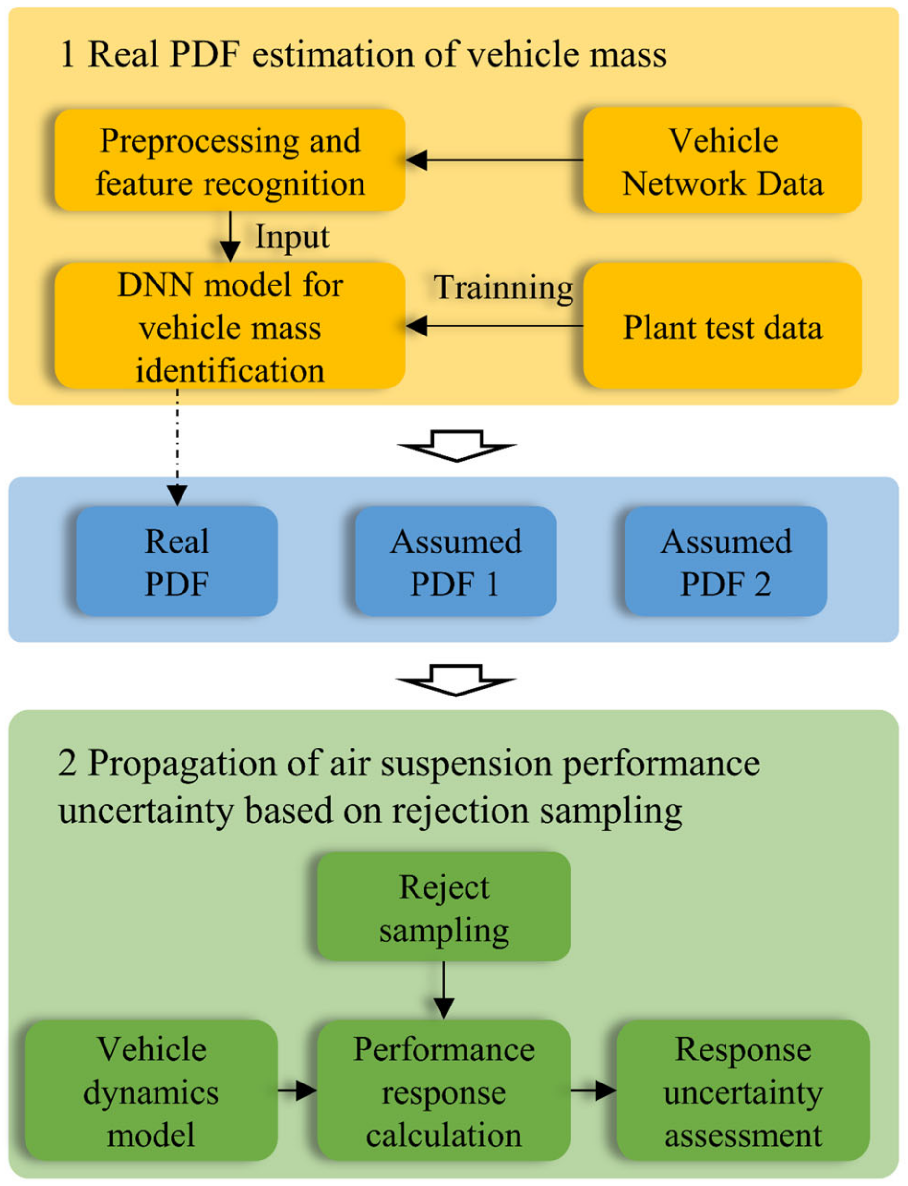
Section 3 can be used as the basis for the uncertainty analysis of the air suspension system. Accordingly, a data-driven bus air suspension system uncertainty analysis can be carried out, the process of which is shown in
Figure 11 and consists of two main steps: 1 is the identification of the whole vehicle mass based on the vehicle network data; and 2 is the air suspension system uncertainty analysis based on rejection sampling. The identified bus masses are used for the statistical true mass probability density function. In addition, as a comparison, two standard mass probability densities are assumed. The three mass probability densities are used as input for the uncertainty analysis of the air suspension system, and the uncertainty of the response is evaluated separately.
4.1. Uncertainty Analysis Based on the Rejection Sampling Principle
In order to make full use of the statistical mass probability distribution information, the empirical probability density of the mass is sampled directly. Acceptance–rejection sampling is able to sample arbitrary probability density functions and it is more efficient when compared to the Monte Carlo sampling method. Therefore, the acceptance–rejection sampling method is used to sample the PDFs of the masses under the three statistical approaches.
Acceptance–rejection sampling principle: is the known target PDF, building a proposed PDF , which makes when , M is constant, where is called the envelope function. Samples and u are generated from and uniform distribution , respectively. Subsequently, we determine whether holds, we accept the sample point if it is established, and we reject the sample point if not. According to the sampling principle, it can be found that, in addition to being able to sample any PDF, rejection sampling and the same sample point may also be accepted by more than one PDF, and therefore can partially circumvent the disadvantages of repeated sampling by the Monte Carlo method.
Two types of pavement profile excitation are used in this paper: sinusoidal excitation and full band excitation. For the sinusoidal excitation, a signal with an amplitude of 0.05 m and a frequency of 1 Hz is used for the simulation. Statistical indicators of the output response for each excitation are also derived.
4.2. Uncertainty Analysis under Sinusoidal Inputs
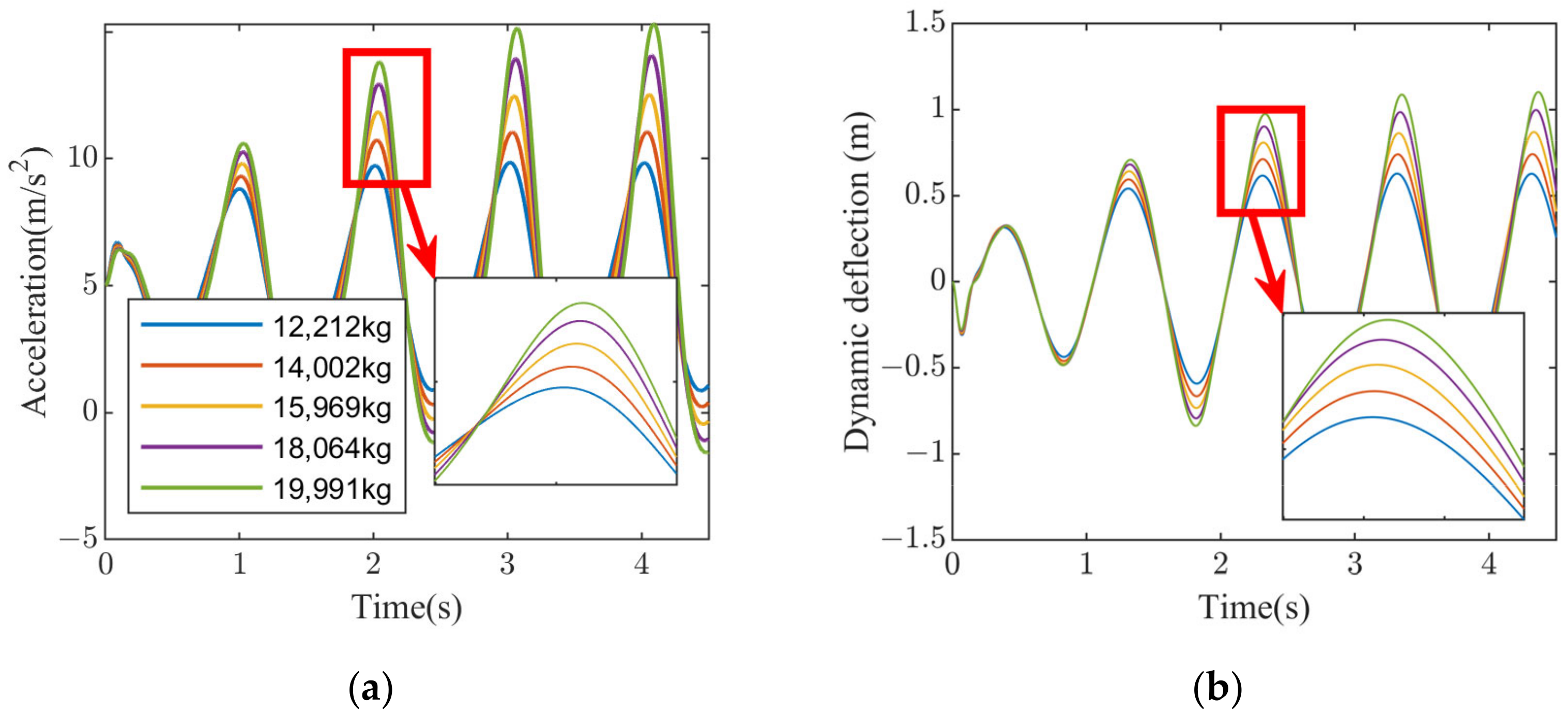
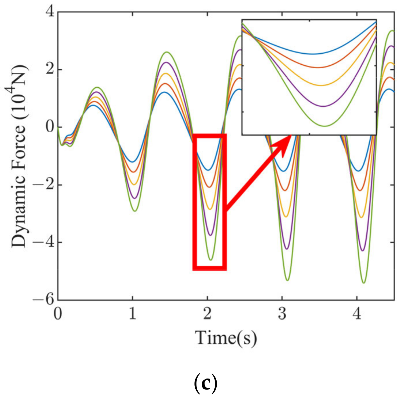
For sinusoidal inputs, Real, Ass1 and Ass2 are used as uncertainty inputs and the output responses of the corresponding performance variables are shown in
Figure 12,
Figure 13 and
Figure 14.
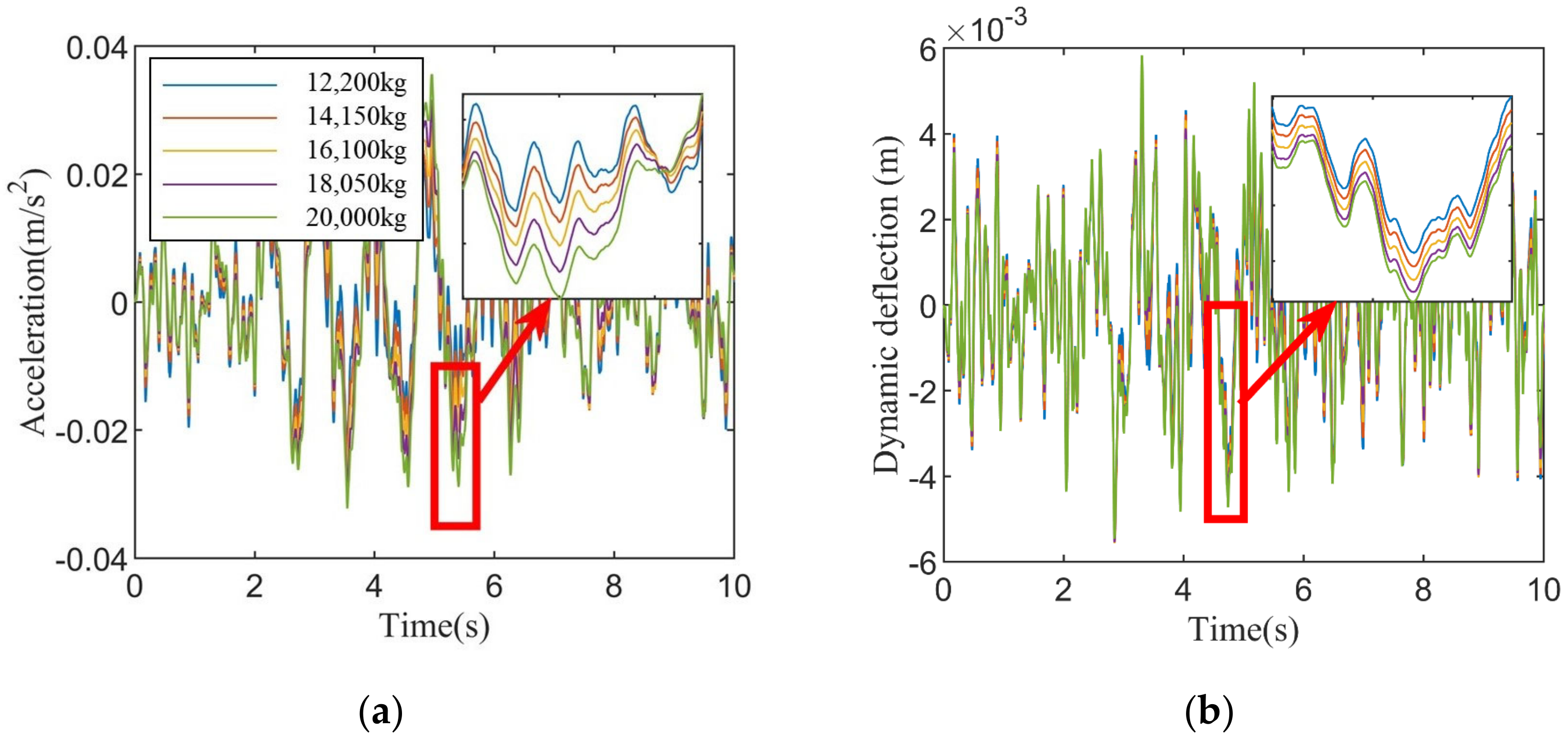
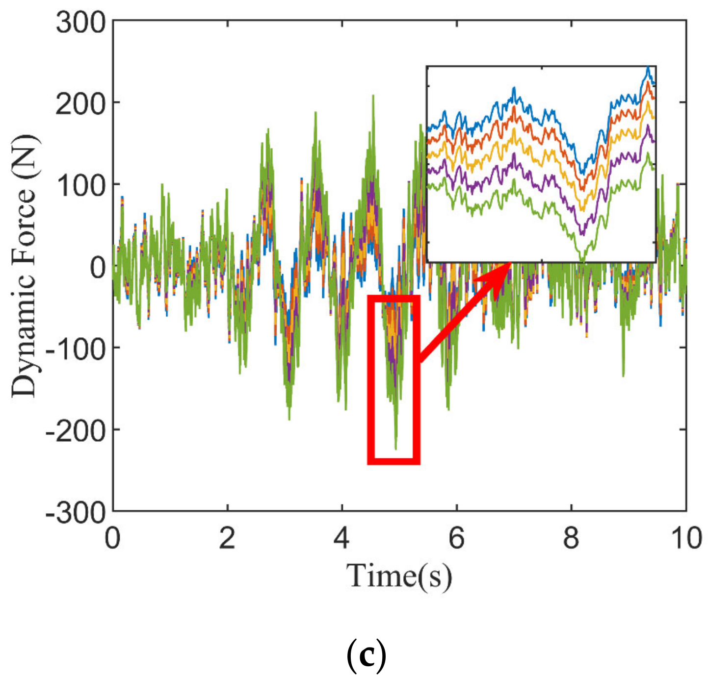
Figure 12 shows the uncertainty response of the three performance metrics of the suspension system based on the true probability density of masses under sinusoidal excitation. Each curve represents the performance response of one type of sprung mass. The sprung mass acceleration, suspension dynamic deflection and wheel dynamic load have similar characteristics, with large differences in y-values for different masses at the peak and trough locations of the response. This indicates that the sprung mass has a large influence on the suspension performance.
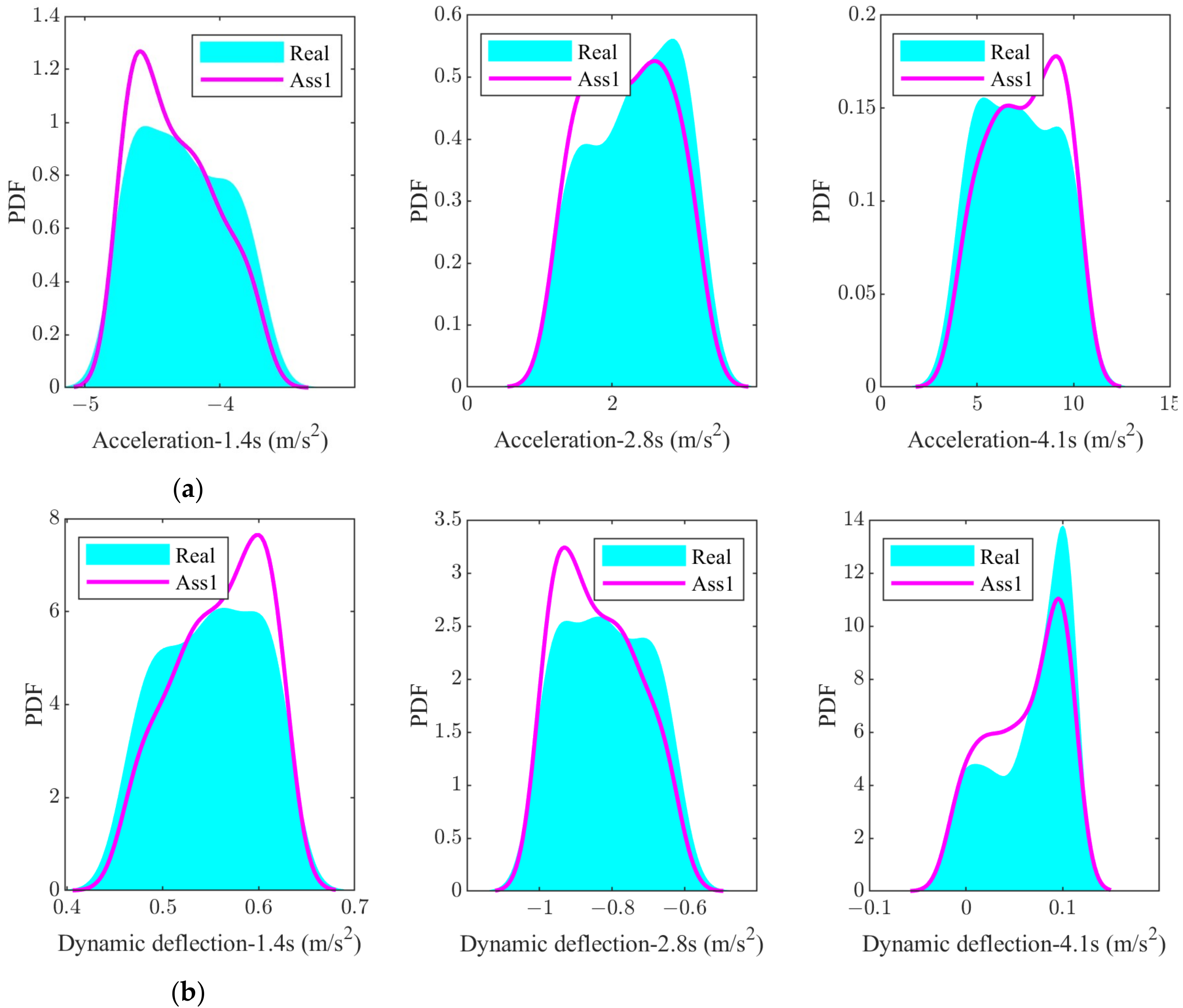
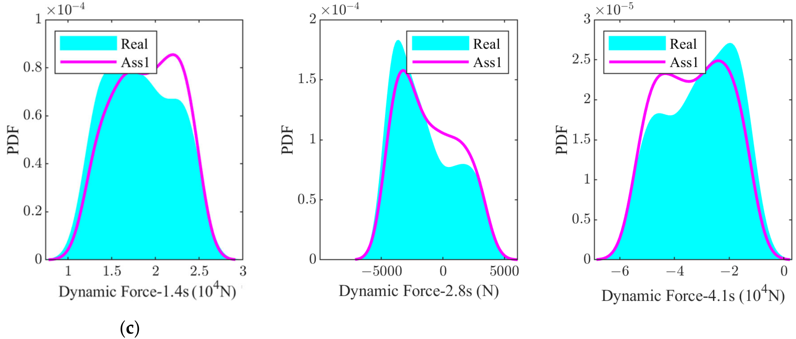
In order to further analyse the influence of the assumed mass distribution and the real mass distribution on the uncertainty response of the suspension performance, the assumed mass PDF and the real mass PDF are used as inputs for the uncertainty analysis of the suspension system; the PDFs of the three responses at the moments 1.4 s, 2.8 s and 4.1 s are calculated, and the results are shown in
Figure 13. It can be found that there are moments where the PDF distributions of the two are similar in shape but different in density value, such as the 1.4 s instant of the acceleration response of sprung mass, the 4.1 s instant of the dynamic deflection of the suspension and the 2.8 s instant of the dynamic wheel load. At other moments, the shape of the PDF distribution and the density values are different.
The mean, standard deviation and variance are important indicators for uncertainty analysis. We calculated the mean and variance of the three performances under the real PDF and the hypothetical PDF, based on mass. Where MVR is the maximum value of the mean of the response and MMR is the maximum value of the variance of the response, the MVR and MMR values for each performance are shown in
Table 4, where the relative error between the hypothetical and true values is shown in brackets and denoted by RE. As can be seen from the table, there is a gap between the MVR and MMR values for the two hypothetical mass distributions and the true mass distribution, and the gap is greater for hypothesis 1, with a maximum relative error of 9% for the dynamic load.
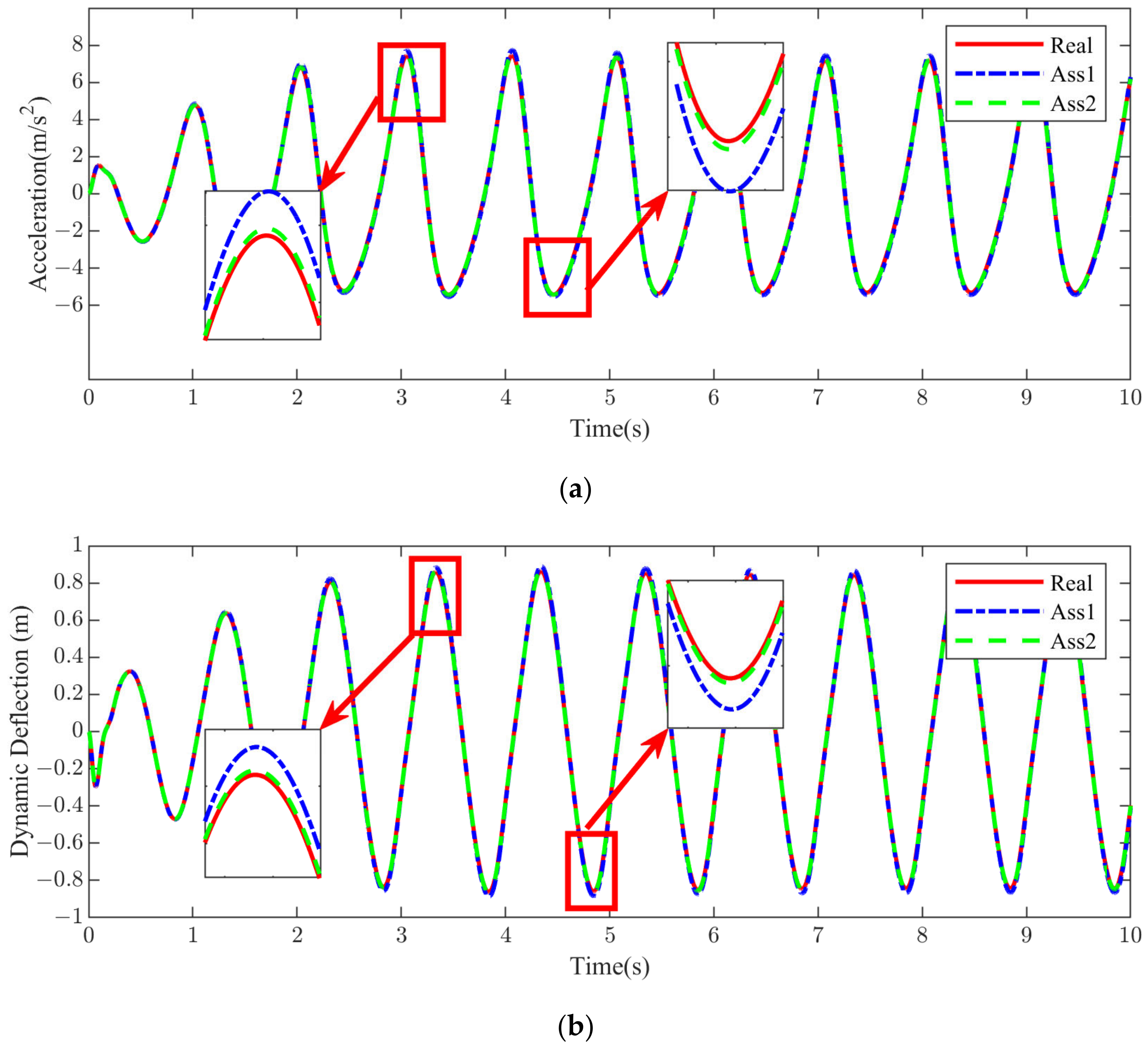
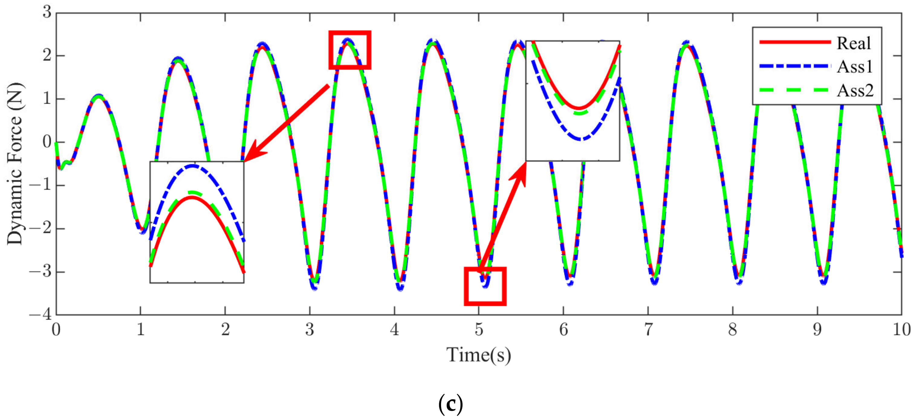
Figure 14 shows a comparison of the performance response for the three mass probability densities. Similar conclusions to those in
Table 4 can be drawn from the local zoomed-in plots, with the performance curve for assumption 1 being highest at the crest and lowest at the trough, indicating that there is a large gap between the performance response based on assumption 1 and the true performance response.
4.3. Uncertainty Analysis under Full Frequency Band Excitation
The frequency response function is an important tool for studying the vibration isolation performance of vibration isolation systems, and the frequency response needs to be obtained from response data under different frequency excitations. The full band excitation is generally modelled using the random white noise of Equation (9). Because the frequencies of interest for suspension systems are low, it is generally sufficient to study the frequency response performance below 30 Hz. To facilitate analytical calculations, we used a range of sinusoidal inputs to study the frequency response characteristics of the suspension system properties, so a series of sine waves with a frequency range of 0–30 Hz and a frequency interval of 0.1 Hz was used as the road excitation. The uncertainty response of the suspension system performance was then calculated using the calculated-true-mass PDF as the uncertainty input.
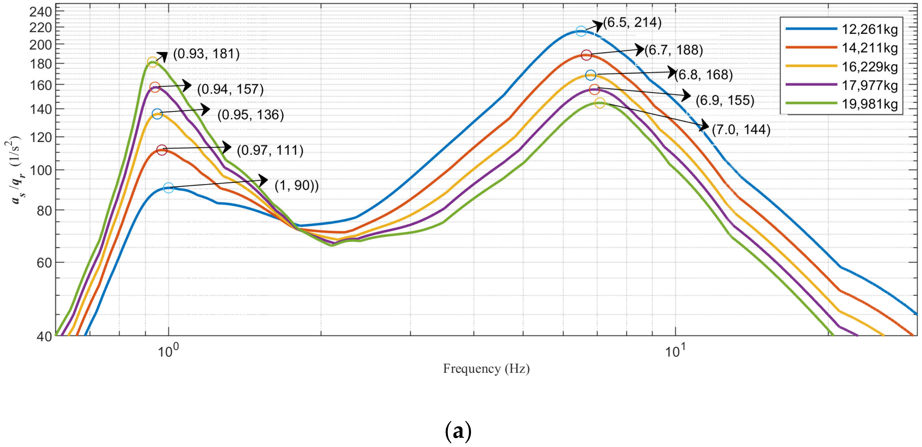
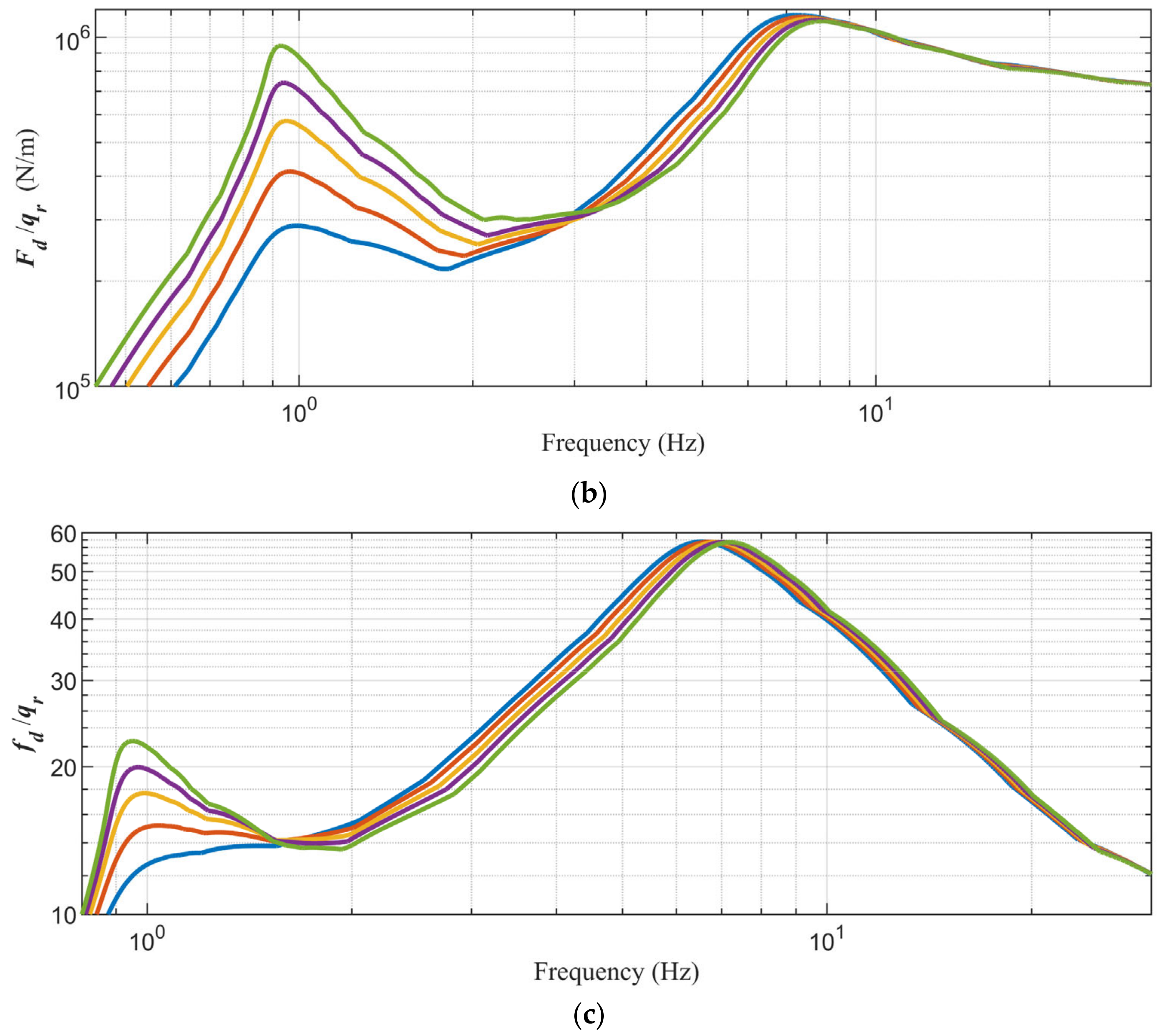
Figure 15 shows the frequency response function curves for the suspension performance for 0–30 Hz excitation.
Figure 15a reveals that the frequency response function of the mass acceleration on the spring fluctuates throughout the frequency band, and has the largest fluctuation range at the resonance peak. The first-order resonance peak frequency and the second-order resonance peak frequency shift with the change in mass. Similarly to
Figure 15b,c, the suspension dynamic deflection and wheel dynamic load fluctuate more in the lower frequency band, but less in the higher frequency band. In summary, the mass acceleration on the spring is more sensitive to mass uncertainty in the full frequency band, while the suspension dynamic deflection and wheel dynamic load are sensitive to mass uncertainty in the low frequency band and insensitive to mass uncertainty in the high frequency band.
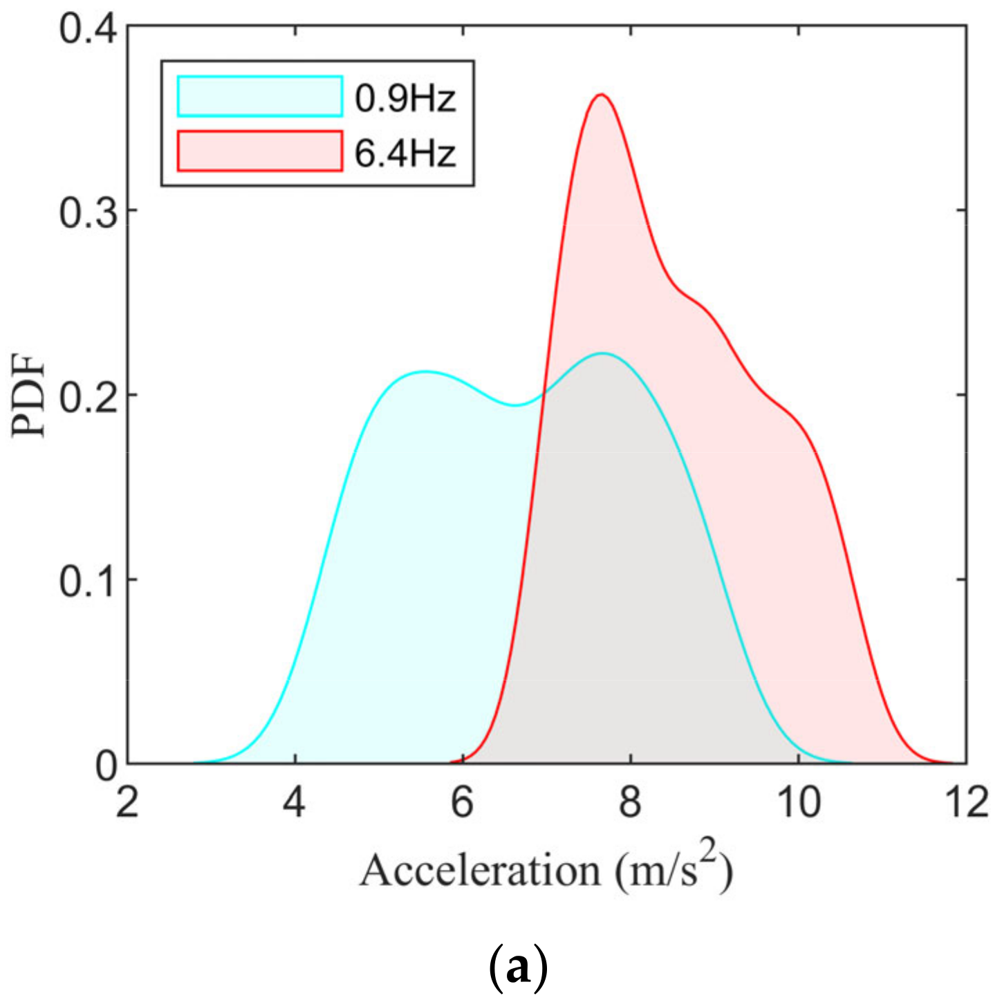
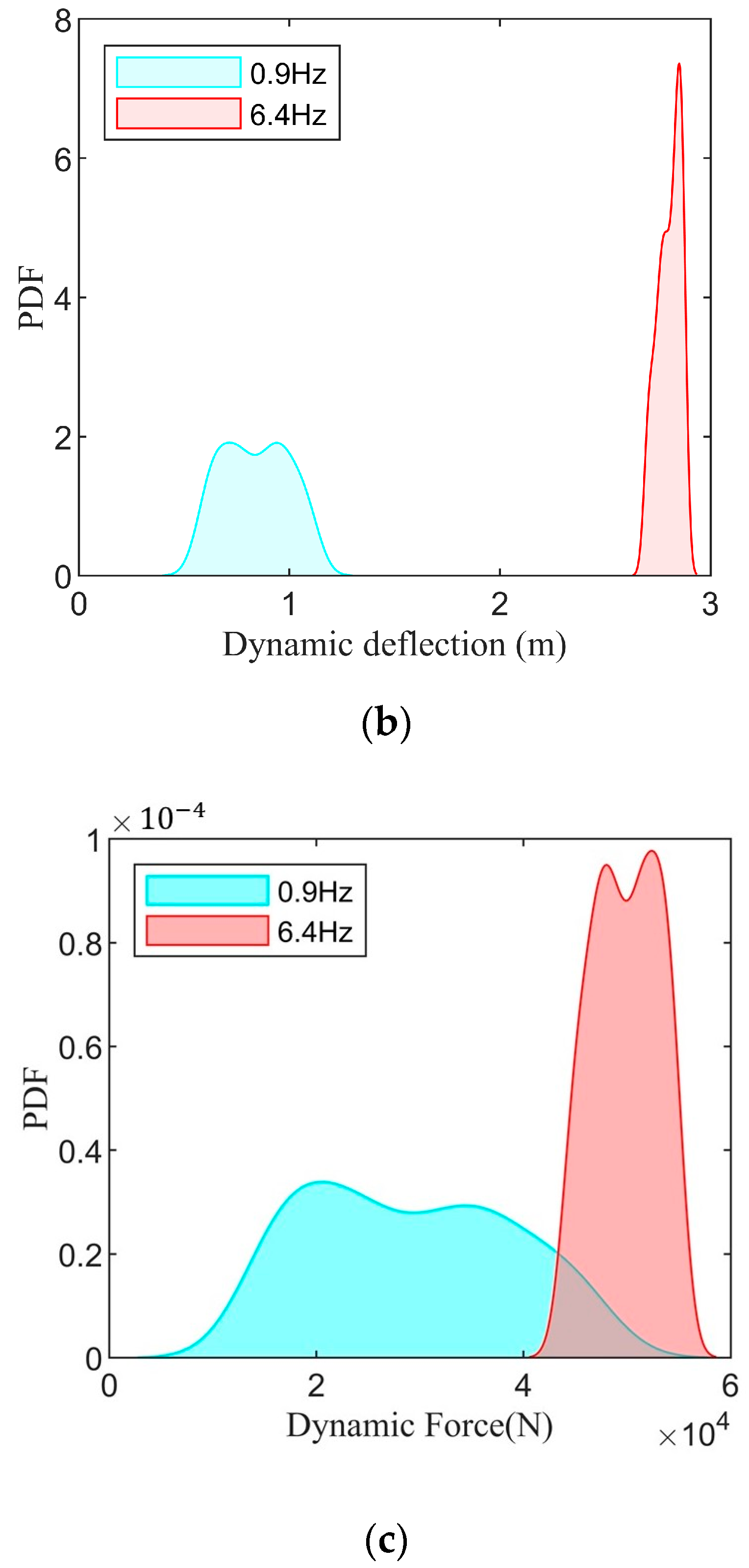
To further quantify the effect of mass uncertainty on suspension performance, the PDFs of the three performance indicators near the two resonance peaks were calculated, as shown in
Figure 16. It can be found that the peak of the curves near the resonance peaks follow the influence of the change in resonance frequency. The approximate distribution range of the peak response near each resonance peak can be confirmed by
Figure 16.
5. Conclusions
This research utilizes the actual probability density of the sprung mass as an input for conducting uncertainty analysis on the air suspension system. Experimental data is employed to train a deep neural network model for accurate mass identification, while vehicle network data are utilized to facilitate the identification and statistical analysis of the sprung mass for a city bus. Subsequently, the rejection sampling principle is applied to sample the true probability density function of the sprung mass, enabling the uncertainty analysis of the air suspension system. The key findings are summarized as follows:
(1) The sprung mass exerts a notable impact on both the natural frequency and amplitude of the suspension system uncertainty response, particularly in the lower frequency ranges. Thus, it is essential to consider the influence of the sprung mass when designing suspension parameters. The trained deep neural network model for mass identification exhibits high accuracy, achieving a maximum error of 5.3%. This level of precision fulfills the requirements for conducting uncertainty analyses of suspension systems.
(2) The probability distribution characteristics of the sprung mass significantly impact the uncertainty response of suspension system performance. It is important to note that assuming a probability distribution might lead to inaccurate calculations of suspension performance uncertainties. In fact, the calculated results for dynamic wheel loads can deviate by up to 9% from the true probability distribution. To acquire precise distributions of uncertainty responses, it is crucial to acquire an accurate sprung mass probability density.
This paper contributes to the field of modeling and analysis of uncertainty parameters in the air suspension system of buses, with a specific focus on the modeling of uncertain mass parameters in buses. The probability distribution characteristics of the sprung mass play a crucial role in determining the distribution characteristics of the suspension performance uncertainties. It is vital to utilize the true probability density function of the sprung mass during the analysis and design of city bus suspension systems. Moving forward, our future work aims to enhance the uncertainty optimization of the air suspension system by leveraging the true probability density function of the sprung mass.


