Article

Design of Radial-Inflow Turbines for Low-Temperature Organic Rankine Cycle

1
Liyang Research Institute, Southeast University, Liyang 213300, China
2
School of Electrical Engineering, Southeast University, Nanjing 210096, China
*
Author to whom correspondence should be addressed.
Machines 2023, 11(7), 725; https://doi.org/10.3390/machines11070725
Submission received: 1 June 2023 / Revised: 26 June 2023 / Accepted: 4 July 2023 / Published: 9 July 2023
(This article belongs to the Special Issue Aerodynamic Design and Optimization for Turbomachinery)

Abstract

:
This study presents the development of a design method that has been extended to the design of radial-inflow turbines operating in organic Rankine cycles (ORC). Both the conventional design method and the circulation method available in the literature have been reviewed. The two main limitations of the current circulation method that make it not suitable for the ORC turbine design are the lack of real gas capability and 3D blades with high stresses. Using the circulation method, the flow field is decomposed into a potential part and a rotational part. The mean velocity field and the periodic velocity field are solved separately. To model the thermodynamic properties of the real gas, NIST REFPROP or CoolProp are used. The blade geometry is then solved iteratively by assuming that the velocity vector is parallel to the blade surface. The blade boundary condition is modified to force the blade camber to be radial-fibred, which is helpful to reduce the centrifugal bending stress on the blade. All the formulations are derived step by step, and the numerical treatments, including grid generation, numerical differentiation, computational scheme, and convergence, are discussed in detail. This method is validated by designing a R245fa ORC turbine rotor. The performance of the rotor design is predicted by CFD and FEA simulations, and it is compared to the results using other methodologies in the literature.

1. Introduction

The organic Rankine cycle is a special variation of the Rankine cycle, which is named for its use of organic, high-molecular-mass fluids whose vaporization temperature is lower than that of water. The main advantage of ORC is that it is suitable for extracting energy from low-grade heat sources compared to the conventional Rankine cycle. One of the earliest research projects about ORC was carried out by Tabor and Bronicki in the 1960s [1]. They designed and tested several small solar ORC systems with monochlorobenzene as the working fluid, and the system power outputs were 2 kW and 10 kW. Since then, ORC has been widely used for heat recovery from low-temperature sources, including biomass combustion [2,3,4], geothermal heat [5,6], industrial waste heat [7,8], and solar thermal heat [9,10,11,12]. The working fluid used in the ORC system plays a very important role in the overall cycle efficiency. Hung et al. [13] compared the thermophysical properties of wet and dry working fluids used in the ORC, while the fluids were characterized based on their slope of saturation vapor diagram. Dai et al. [14] compared different working fluids for high-temperature ORC systems, and Usman et al. [15] performed a comparative study on the low-medium-temperature geothermal ORC system using R245fa and R1233zde. Pang et al. [16] carried out an experiment to compare using R245fa, R123, and their mixtures with varying mass fractions in the ORC systems. Eyerer et al. [17] experimentally investigated modern ORC working fluids R1224yd(Z) and R1233zd(E) as replacements for R245fa.
Turbines or expanders are another important part of the ORC system. Radial-inflow turbines, scroll expanders, and screw expanders are typically used. The most favorable or widely used turbine nowadays is the radial-inflow turbine due to its light weight and high efficiency. However, the cost of radial-inflow turbines will be higher than others. Different researchers have tried to design and use radial-inflow turbines in the ORC [18,19,20,21,22]. The method they used for the design of radial-inflow turbines is called the conventional method. The initial leading edge (LE) and trailing edge (TE) blade angles are calculated based on 1D meanline analysis and velocity triangles. A smooth cubic spline or Bezier curve would be used to define the blade angle or wrap angle distribution along the streamwise direction. The wrap angle at other spanwise locations (from hub to shroud) will be obtained through radial filament, which minimizes the blade’s centrifugal bending stress. The 3D blade geometry is constructed by lofting all the sections together, and CFD simulations or experiments will be used to evaluate the turbine’s performance.
A different method called the circulation method (or inverse design method) was first proposed by Hawthorne et al. [23], and they used it to design infinitely thin 2D cascades for inviscid and incompressible flow. The cascade blade is modeled as a single vorticity sheet using this method, and the blade shape is calculated iteratively by using the boundary condition that the flow is assumed to be parallel to the blade surface. Tan et al. [24] extended this method to the design of 3D cascades with constant hub and shroud diameters. One limitation of their method is that the blade is still assumed to be infinitely thin (zero blade thickness). Borges [25] extended Tan’s method further to the design of low-speed turbomachinery with arbitrary meridional geometry, which makes it possible to design centrifugal and mixed-flow pumps using this method. Ghaly [26] added flow compressibility to this method and used it to design radial-inflow turbines with compressible and subsonic flow. The blade thickness effect was then introduced by Zangeneh [27] using a blockage factor in the mean flow continuity equation. Since then, the circulation method has been widely used for the design of a very wide range of turbomachinery blades, including compressors [28], fans [29], pumps [30], and hydraulic turbines [31].
To apply the existing circulation method to the design of radial-inflow turbines for ORC, there are two main limitations. The first is that the flow has been assumed to be incompressible or compressible ideal gas, while the ORC working fluid is real gas. Therefore, the ideal gas assumption does not hold any more. Colonna et al. [32] investigated the real gas effect in ORC turbines by comparing the polytropic ideal gas law, the Peng–Robinson–Stryjek cubic equation of state (EoS) and the Span–Wagner EoS. The second limitation is that the blade designed using the circulation method has quite high stress due to its complex 3D blade shape. To control the stress within allowable material strength, post-modifications, including modifying the blade thickness or wrap angle distribution (radial filament modification), are required to convert the blade to be radial-filament or radial-fibred blading.
In this paper, a design method that can be used to design radial-inflow turbines with real gas (organic) fluids and generate radial-filament geometries directly is proposed. The performance of the radial-inflow turbine will be evaluated and validated through 3D CFD and FEA simulations.

2. Methodology and Governing Equations

2.1. Basic Assumptions

First, the following assumptions are made:
  • The flow is assumed to be adiabatic, steady, and inviscid;
  • The fluid is compressible and a real gas;
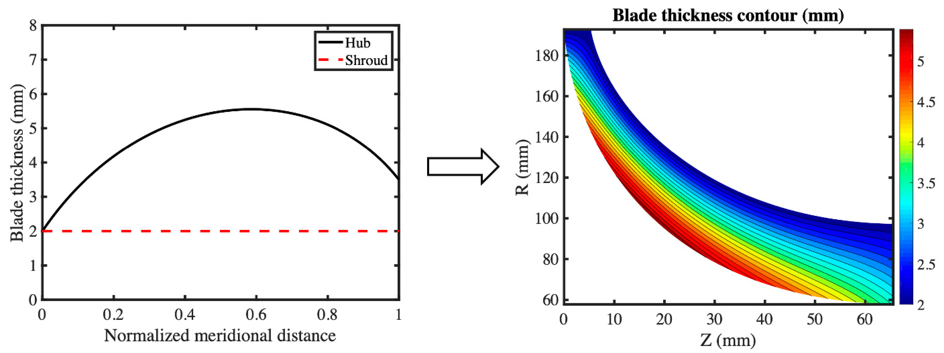
  • The blade is assumed to be infinitely thin with zero blade thickness;
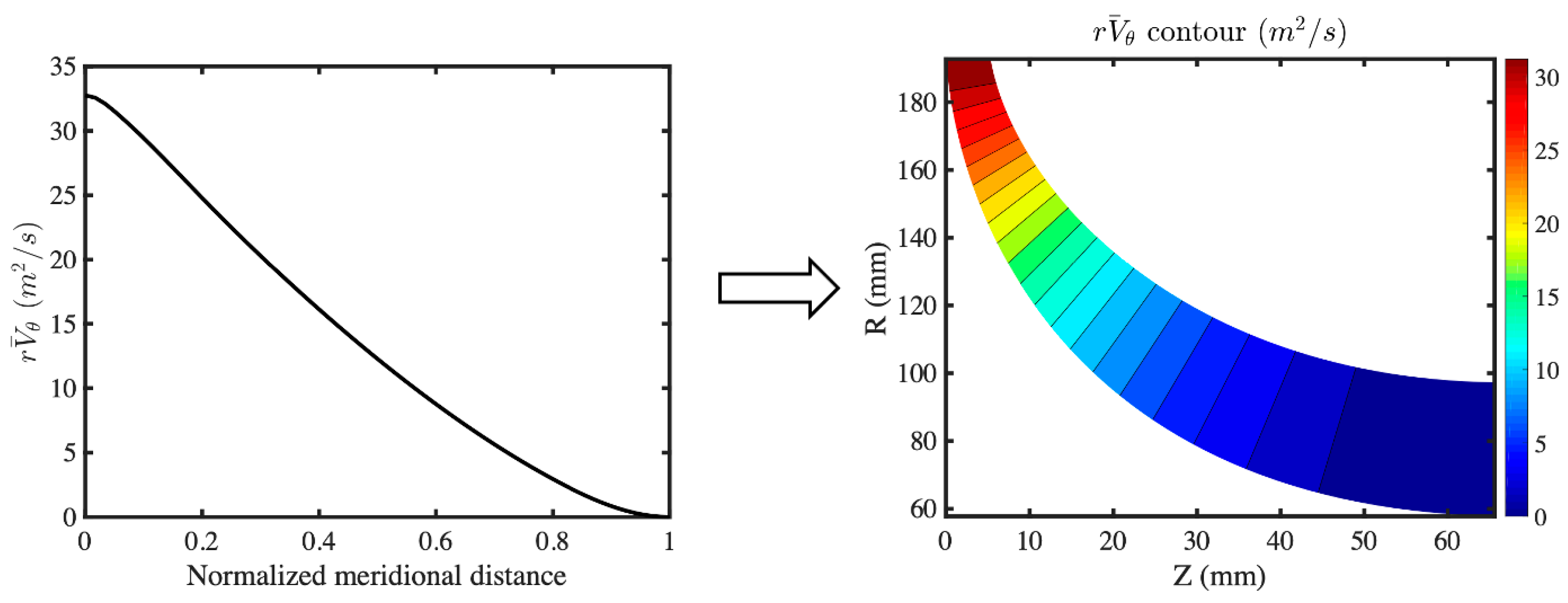
  • The flow near TE is free vortex, which means there is no vortex shedding after TE.
Using the first assumption with Kelvin’s theorem, it can be concluded that the only vorticity in the flow field is the blade-bound vorticity, which is bounded on all the blade surfaces. Because of the assumption of infinitely thin blades, one vorticity sheet can be used to represent the blade geometry. A blockage factor is used in the mean flow continuity equation to account for the blockage effect caused by the blade thickness.
The blade camber (or wrap angle) can be defined by:
α r , θ , z = θ f r , z = ± n 2 π B
where α is all the blade surfaces, r, θ, and z are cylindrical coordinates, f is the blade camber, and B is the blade number. It should be noted that f represents the wrap angle of one single blade, while α represents the wrap angles of all the blades.
The overbar symbol ‘−’ is used to define a way of averaging along the circumferential direction, for example:
A ¯ r , z = 2 π B 0 2 π B A r , θ , z d θ
To model the periodic flow properties, a Dirac delta function is used:
n = δ α n 2 π B = +                     α = n 2 π B 0                             α   n 2 π B
It can be easily seen that the value of the delta function is infinite on the blade and remains zero anywhere else. Equation (3) can be rewritten in the form of a Fourier series (Lighthill [33]):
δ P α = 2 π B n = δ α n 2 π B = n = e i n B α
The vorticity field can then be defined by Equation (5). It should be noted that the vorticity is periodic along the circumferential direction and only holds non-zero values on all the blade surfaces.
Ω r , θ , z = Ω ¯ r , z δ P α

2.2. Monge–Clebsch Decomposition

The Monge–Clebsch decomposition is used to decompose the velocity field into the summation of a potential term and a rotational term (Wu et al. [34]).
V r , θ , z = Φ r , θ , z + λ r , θ , z μ r , θ , z
where ∇Φ is the potential term and λμ is the rotational term. Taking the curl of Equation (6) to obtain the vorticity:
Ω r , θ , z = λ r , θ , z × μ r , θ , z
One of the Clebsch variables can be assumed to be α. Therefore, Equation (7) can be rewritten as:
Ω r , θ , z = λ r , θ , z r , λ r , θ , z r θ , λ r , θ , z z × f r , z r , 1 r , f r , z z
The mean vorticity field Ω   can be obtained by taking the circumferential average of both sides of Equation (8).
Ω ¯ r , z = λ ¯ r , z r z , λ ¯ r , z r f r , z z λ ¯ r , z z f r , z r , λ ¯ r , z r r
Taking the circumferential average of the velocity curl to obtain the mean vorticity Ω ¯ :
Ω ¯ r , z = r V ¯ θ   r , z r z , V ¯ r   r , z z V ¯ z   r , z r , r V ¯ θ   r , z r r
By comparing Equations (9) and (10), it can be easily seen that:
λ ¯ r , z = r V ¯ θ   r , z
Equations (5) and (9) can then be rewritten as:
Ω r , θ , z = r V ¯ θ r , z × α r , θ , z δ P α
Ω ¯ r , z = r V ¯ θ r , z × α r , θ , z
A periodic sawtooth function S α   can be defined by Equations (14) and (15).
S α = δ P α 1 = n = e i n B α 1 = 2 n = 1 e i n B α
S α = 2 n = 1 e i n B α i n B + C
Using Equations (12), (14) and (15), the absolute vorticity field Ω   can be written in the following form:
× V r , θ , z = Ω r , θ , z = × Φ r , θ , z + r V ¯ θ r , z α r , θ , z S α r V ¯ θ r , z
The velocity field V can then be expressed by the following equation.
V r , θ , z = Φ r , θ , z + r V ¯ θ r , z α r , θ , z S α r V ¯ θ r , z
The velocity field can also be expressed by the summation of a mean term and a periodic term.
V r , θ , z = V ¯ r , z + V ~ r , θ , z
Comparing Equations (17) and (18), the equations for the mean flow velocity V ¯ and the periodic flow velocity V ~ can be obtained.
V ¯ r , z = Φ ¯ r , z + r V ¯ θ r , z α r , θ , z
V ~ r , θ , z = Φ ~ r , θ , z S α r V ¯ θ r , z
where Φ ¯ is the mean flow potential function and Φ ~ is the periodic flow potential function. The last terms on the RHS of Equations (19) and (20) are equal to zero in the inlet and outlet regions since the flow is irrotational.

2.3. Continuity Equations

The typical steady and compressible flow continuity equation can be written in the following form:
· ρ r , θ , z W r , θ , z = 0 · W r , θ , z = W r , θ , z · l n ρ r , θ , z    
To obtain the mean flow continuity equation, we can take the circumferential average on both sides of Equation (21).
𝛻 · W ¯ r , z = W r , θ , z · 𝛻 l n ρ r , θ , z ¯
The relative velocity W can be written in the following form:
W r , θ , z = W ¯ r , z + V ~ r , θ , z
To obtain the periodic flow continuity equation, we can take the divergence of Equation (23) and compare it with Equations (21) and (22).
𝛻 · V ~ r , θ , z = W r , θ , z · 𝛻 l n ρ r , θ , z + W r , θ , z · 𝛻 l n ρ r , θ , z ¯

2.4. Mean Flow Equations

2.4.1. Blockage Effect

The blade thickness at the hub section of a typical radial-inflow turbine is quite large, and its blockage effect should not be neglected. A blockage factor B f is introduced into the continuity equation for the mean flow to account for the blockage effect caused by the finite blade thickness.
𝛻 · ρ m r , z B f r , z W ¯ r , z = 0
where ρ m is a special artificial density, which will be discussed in the next subsection. B f is defined as:
B f r , z = 1 t θ r , z B 2 π r
where t θ is the tangential thickness distribution for the blade and B is the blade number. The relation between the blade’s normal thickness and the tangential thickness is defined by Equation (27). It is more common to directly define the blade’s normal thickness for stress considerations.
t θ r , z = t N r , z 1 + r 2 f r , z m 2

2.4.2. Artificial Density

A special artificial density ρ m   is defined (Equation (25)) so that the mean flow velocities can be solved through a Stokes stream function for 3D axisymmetric flow. ρ m   can be calculated through Equations (22) and (25):
W ¯ r , z · 𝛻 l n ρ m r , z = W r , θ , z · 𝛻 l n ρ r , θ , z ¯ W ¯ r , z · 𝛻 l n B f r , z
To simplify equations later, ρ m is normalized by a constant reference density ρ i (e.g., inlet stagnation density) to obtain ρ a :
ρ a r , z = ρ i ρ m r , z

2.4.3. Stokes Stream Function

To solve the mean flow continuity equation (Equation (25)), a stream function Ψ for axisymmetric flow can be defined:
W r ¯ r , z = V r ¯ r , z = ρ a r , z r B f r , z Ψ r , z z W z ¯ r , z = V z ¯ r , z = ρ a r , z r B f r , z Ψ r , z r
The stream function Ψ satisfies the mean flow continuity equation Equation (25) automatically. Another equation is required to solve the unknown stream function Ψ. Comparing Equations (9) and (10), it can be concluded that:
V ¯ r   r , z z V ¯ z   r , z r = r V ¯ θ r , z r f r , z z r V ¯ θ r , z z f r , z r
Substituting Equation (30) into Equation (31) with some rearrangements, the stream function Ψ can be expressed in the following form:
2 Ψ r 2 Ψ r r + 2 Ψ z 2 + Ψ r l n ρ a r l n B f r + Ψ z l n ρ a z l n B f z = r B f ρ a r V ¯ θ z f r r V ¯ θ r f z
where the RHS of Equation (32) remains zero since the flow is irrotational in the upstream and downstream regions of the blade region.

2.4.4. Boundary Conditions

The stream function equation (Equation (32)) is an elliptic partial differential equation that can be solved subject to boundary conditions applied at all the boundaries.
There is no flow passing through the hub and the shroud surface, which means that the flow streamlines align with the hub and the shroud walls. Therefore, the following boundary conditions can be applied at the hub and the shroud:
Ψ r , z = c o n s t
The upstream (inlet) boundary condition is defined by the known velocity at the upstream boundary:
ρ a r , z r Ψ r , z s r , z = V ¯ · n
The velocity at the downstream boundary will be uniform and parallel in the absence of the shed vorticity. This condition is defined as:
Ψ r , z n = 0

2.5. Periodic Flow Equations

To solve the periodic flow equation (Equation (24)), we would first like to obtain the equation for the potential function for the periodic flow Φ ~ . Take the divergence of Equation (20) and substitute Equation (24), and we can get:
𝛻 2 Φ ~ r , θ , z = S α 𝛻 2 r V ¯ θ   r , z + S α 𝛻 α · 𝛻 r V ¯ θ   r , z W r , θ , z · 𝛻 l n ρ r , θ , z + W r , θ , z · 𝛻 l n ρ r , θ , z ¯
where the first two items on the RHS remain zero in the inlet and outlet regions, the last two items on the RHS require the calculation of the full 3D velocity field and density field. Due to the fact that the flow is periodic along the circumferential direction, it is possible to express the potential function for the periodic flow Φ ~   in the form of a complex Fourier series.
Φ ~ r , θ , z = n = , n 0 Φ ~ n r , z e i n B θ
where Φ ~ n   is the Fourier coefficients of the potential function for the periodic flow Φ ~ . The periodic potential function Φ ~ can be further approximated in the form of a truncated IDFT:
Φ ~ r , θ , z n = N 2 N 2 1 Φ ~ n r , z e i n B θ Φ ~ r , θ j , z n = N / 2 N / 2 1 Φ ~ n r , z e i k n θ j
where θ j   is defined by Equation (39) and its value is the tangential coordinate of grid points in the tangential direction. The total number of grids is N and the spacing between grids is ∆θ.
θ j = j θ                 j = 0,1 , 2 , , N
k n   has been chosen to make the function e i k n θ j space equally and periodically.
k n = n B = 2 π n N θ                 n = N 2 , , 1,0 , 1 , , N 2 1
Using Equations (36), (38)–(40), the periodic flow potential function can be expressed in the following form:
2 Φ ~ n r 2 + Φ ~ n r r + 2 Φ ~ n z 2 n 2 B 2 r 2 Φ ~ n = e i n B f i n B 𝛻 2 r V ¯ θ e i n B f 𝛻 f · 𝛻 r V ¯ θ + F n n = N 2 , , 1,0 , 1 , , N 2 1
where F n is the Fourier coefficient of W · 𝛻 l n ρ + W · 𝛻 l n ρ ¯ . The terms when n = 0 need to be neglected for the solution of the periodic flow since they represent the Monge–Clebsch formulation of the mean flow equation. Therefore, Equation (41) becomes:
2 Φ ~ n r 2 + Φ ~ n r r + 2 Φ ~ n z 2 n 2 B 2 r 2 Φ ~ n = e i n B f i n B 𝛻 2 r V ¯ θ e i n B f 𝛻 f · 𝛻 r V ¯ θ R n   n = N 2 , , 1,1 , , N 2 1
where R n is defined as:
R n r , z = 1 N   j = 1 N W r , θ j , z · 𝛻 l n ρ r , θ j , z   e i 2 π n j N
Since the periodic flow potential function is a real function Φ ~ , its Fourier transform satisfies the following equation:
Φ ~ n r , z = Φ ~ n * r , z                 n = 1,2 , , N 2
where * denotes the complex conjugation and only half of the frequency spectra in Equation (42) need to be solved.
In order to solve Equation (42) for Φ ~ n , boundary conditions need to be applied to the four boundaries of the physical domain, including the hub wall, the shroud wall, and the upstream (inlet) and downstream (outlet) boundaries.
The periodic velocity V ~ should align with the hub and the shroud walls, which can be expressed by:
V ~ r , θ , z · n = 0
where n is the unit vector that is perpendicular to the hub or the shroud.
Substituting Equation (20) into Equation (45) and using Equations (15) and (37), the hub and the shroud boundary conditions for the periodic potential function can be obtained:
Φ ~ n r , z n = e i n B f r , z i n B r V ¯ θ r , z n
The flow is uniform at the far upstream and far downstream boundaries, which implies that the periodic velocity vanishes as the flow approaches the upstream/downstream boundaries. This condition can then be expressed in the following form:
Φ ~ n r , z n = 0
The periodic velocity V ~ is computed by using the IDFT (inverse discrete Fourier transform) of Equation (20).
V r ~ r , θ , z = n = N 2 , N 0 N 2 1 Φ ~ n r , z r r V ¯ θ r , z r e i k n f r , z i k n V θ ~ r , θ , z = n = N 2 , N 0 N 2 1 i k n Φ ~ n r , z r V z ~ r , θ , z = n = N / 2 , N 0 N / 2 1 Φ ~ n r , z z r V ¯ θ r , z z e i k n f r , z i k n  

2.6. Calculation of Thermophysical Properties

The thermophysical properties of any real gas can be obtained by calling the NIST REFPROP Fortran subroutine [35] or CoolProp C++ library [36] with any two known thermodynamic properties. The inlet total enthalpy h 01 and inlet entropy s 1 can be obtained from the given inlet total pressure P 01 and inlet total temperature T 01 . The entropy remains constant throughout the whole flow domain since the flow is inviscid and isentropic.
The rothalpy, which is defined by Equation (49), is conserved along any streamline in a steady adiabatic flow.
I = h + 1 2 W 2 U 2 = h 0 ϖ r V θ = c o n s t
where h is the static enthalpy, W is the relative velocity, U is the blade speed, and ϖ is the rotational speed. The inlet rothalpy can be calculated based on the inlet total enthalpy h 01 and the inlet r V ¯ θ value. The total enthalpy value h 0 and static enthalpy h at other locations rather than the inlet can be calculated from the constant rothalpy value I and known r V ¯ θ or relative velocity W at that location. Using the known entropy s and enthalpy h 0 ( h ) with REFPROP or CoolProp, other fluid properties, including density ρ , pressure P and temperature T , at any location can be obtained. It should be noted that all the properties discussed in this section are circumferentially averaged values, which means they are functions of r and z . The static enthalpy jump across the blade can be calculated from Equation (50).
h + r , z h r , z = 2 π B W b l r , z · 𝛻 r V ¯ θ r , z
where h + is the static enthalpy on the blade pressure surface, h is the static enthalpy on the blade suction surface and W b l is the mean blade surface velocity. The mean static enthalpy is known, and it is equal to the mean of h +   and h . Using Equations (50) and (51), h +   and h can be obtained. Similarly, using the constant entropy, the blade surface pressures P + (static pressure on the pressure surface) and P (static pressure on the suction surface) will be obtained.
h r , z = 1 2 h + r , z + h r , z
The 3D enthalpy field h r , θ , z   can be calculated using Equation (49) using rothalpy I and the 3D relative velocity field W r , θ , z . The 3D density field ρ r , θ , z can then be obtained from the constant entropy and h r , θ , z   using REFPROP or CoolProp. The Fourier transform of the natural logarithm of the density field is computed by the following equation once the density field ρ r , θ , z   is available.
ρ n r , z = 1 N j = 1 N ln ρ n r , θ j , z e i 2 π j n N                 θ j = j Δ θ
Taking the IDFT of i k n r ρ n r , z we can get the derivative of ln ρ n r , θ j , z   in the tangential direction. Similarly, to get the axial and radial derivatives of ln ρ n r , θ j , z we need to take the IDFT of the corresponding derivatives of ρ n r , z .
W r , θ , z · 𝛻 l n ρ r , θ , z   can be computed based on the derivatives of ln ρ n r , θ j , z   and the relative velocity field W r , θ , z . The Fourier transform of W r , θ , z · 𝛻 l n ρ r , θ , z is calculated using Equation (43) to obtain R n . The 0th component of Equation (43) which is equivalent to W r , θ , z · 𝛻 l n ρ r , θ , z ¯ will be used in Equation (28) to calculate the artificial density ρ m .

2.7. Calculation of Blade Shape

The blade shape is calculated based on the boundary condition that the relative velocity is parallel to the blade surface.
W b l r , θ , z · α r , θ , z = 0
Substituting Equations (1) and (23) into Equation (53) gives:
V ¯ r + V ~ r , b l f r + V ¯ z + V ~ z , b l f z = r V ¯ θ   r 2 + V ~ θ , b l r ϖ
To solve Equation (54), the initial value of f along a quasi-orthogonal needs to be specified, and this is called the stacking condition. To make the blade radial-fibred, the gradient of the camber f along the radial direction is forced to be zero using Equation (55).
f r = 0

3. Numerical Techniques

3.1. Grid Generation

To numerically solve all the PDEs above, a computational mesh is needed. In the case of irregular-shaped domains (e.g., curved hub and shroud profiles for a turbine rotor), transformation from the physical domain (r–z plane) to a regular (mostly rectangle) computational domain (ξ–η plane) is required. It should be noted that the numerical grid in the θ direction is not needed since the flow equations in the θ direction are solved using the discrete Fourier Transform. Figure 1 below shows an example of this coordinate transformation. It should be noted that the physical domain boundaries/edges (ABCD) do not have to be straight and can be curved or have irregular shapes. The newly generated ξ–η coordinate is called a body-fitted curvilinear coordinate, and its main advantage is that it makes the discretization of PDEs and imposing the boundary conditions more straightforward and simpler compared to solving PDEs on the r–z plane.
Using Equation (56), all the mesh point coordinates can be obtained through transfinite interpolation [37]. The curves c 1 ξ and c 3 ξ   are one pair of opposite sides of the physical domain, and c 2 η and c 4 η   are another pair shown in Figure 1. P 1,2 is the point A where curves c 1 and c 2 intersect.
S ξ , η = 1 η c 1 ξ + η c 3 ξ + 1 ξ c 2 η + ξ c 4 η 1 ξ 1 η P 1,2 + ξ η P 3,4 + ξ 1 η P 1,4 + η 1 ξ P 3,2
A typical meridional geometry of a radial-inflow turbine rotor is shown in Figure 2 and it is divided into three regions, including the inlet region, the blade region, and the outlet region by blade LE and TE. The body-fitted curvilinear mesh for each region can then be generated using the method explained above. The number of streamwise grid points (along ξ direction) in each region is proportional to its averaged meridional length, which will result in a relatively uniform grid size along the streamwise direction.

3.2. Transformed Equations in Curvilinear Coordinates

Once the numerical grid is ready, the equations described in Section 2 need to be transformed from (r,z) coordinates to (ξ,η) coordinates using the method described by Thompson et al. [38], which is shown in Appendix A.
Equation (32) is transformed into:
α Ψ ξ ξ 2 β Ψ ξ η + γ Ψ η η + τ + z η J r + α ln ρ a ξ ln B f ξ β ln ρ a η ln B f η Ψ ξ + σ z ξ J r + γ ln ρ a η ln B f η β ln ρ a ξ ln B f ξ Ψ η = J r B f r V ¯ θ ξ f η r V ¯ θ η f ξ / ρ a
Mean velocities V ξ ¯ and V η ¯   can be calculated using the following equations:
V ξ ¯ ξ , η = J ρ a ξ , η r B f ξ , η Ψ r , z η V η ¯ ξ , η = J ρ a ξ , η r B f ξ , η Ψ r , z ξ
Equation (42) is transformed into:
α Φ n ξ ξ 2 β Φ n ξ η + γ Φ n η η + τ z η J r Φ n ξ + σ + z ξ J r Φ n η J 2 n 2 B 2 r 2 Φ n = J 2 e i n B f ξ , η i n B α r V ¯ θ ξ ξ + γ r V ¯ θ η η 2 β r V ¯ θ ξ η + τ r V ¯ θ ξ + σ r V ¯ θ η J 2 e i n B f ξ , η f ξ α r V ¯ θ ξ β r V ¯ θ η + f η γ r V ¯ θ η β r V ¯ θ ξ J 2 R n ξ , η
where R n ξ , η   is calculated by the following equation.
R n ξ , η = 1 N   j = 1 N W ξ , θ j , η · 𝛻 l n ρ ξ , θ j , η   e i 2 π n j N
Blade boundary conditions, Equations (54) and (55), are transformed into:
V ¯ ξ + V ~ ξ , b l f ξ + V ¯ η + V ~ η , b l f η = J 2 r V ¯ θ   r 2 + V ~ θ , b l r ϖ z ξ f η z η f ξ = 0
where the periodic blade surface velocities V ~ ξ , b l , V ~ η , b l and V ~ θ , b l   can be calculated by Equation (62) and are shown below.
V ~ ξ , b l ξ , η = n = N 2 , N 0 N 2 1 α Φ n c ξ β Φ n c η cos n B f α Φ n s ξ β Φ n s η sin n B f V ~ η , b l ξ , η = n = N 2 , N 0 N 2 1 γ Φ n c η β Φ n c ξ cos n B f γ Φ n s η β Φ n s ξ sin n B f V ~ θ , b l ξ , η = n = N 2 , N 0 N 2 1 n B r Φ n c sin n B f + Φ n s cos n B f
It should be noted that only the real part of the function is kept since the velocity is a real function. Therefore, the superscript ‘c’ indicates the real part of the function, and the superscript ‘s’ indicates the imaginary part of the function.

3.3. Numerical Differentiation

The elliptic Equations (57) and (59) are discretized by using central difference at the internal points and second-order upwind/downwind at the boundary points (inlet, outlet, hub, and shroud). Assuming a uniform grid in the transformed computational domain ( Δ ξ = Δ η ), for any point (j,k), where j is the point index along the ξ direction and k is the point index along the η direction, the derivatives of a function F(ξ,η) can be expressed in the following forms:
F ξ j , k = F ξ , η ξ = 1 2 F j + 1 , k F j 1 , k F η j , k = F ξ , η η = 1 2 F j , k + 1 F j , k 1 F ξ ξ j , k = 2 F ξ , η ξ 2 = F j + 1 , k 2 F j , k + F j 1 , k F η η j , k = 2 F ξ , η η 2 = F j , k + 1 2 F j , k + F j , k 1 F ξ η j , k = 2 F ξ , η ξ η = 1 4 F j + 1 , k + 1 F j + 1 , k 1 + F j 1 , k 1 F j 1 , k + 1
The above discretization equations are second-order accurate. For the boundary points (inlet, outlet, hub, and shroud), second-order upwind/downwind difference schemes are used similarly.
The first-order hyperbolic Equation (61) is discretized by using the central difference at the fictitious point (j+1/2,k) with second-order accuracy and the derivatives of a function F(ξ,η) can be expressed in the following forms:
F ξ j + 1 2 , k = F ξ , η ξ = F j + 1 , k F j 1 , k F η j + 1 / 2 , k = F ξ , η η = 1 4 F j , k + 1 F j , k 1 + F j + 1 , k + 1 F j + 1 , k 1
Equation (28) that solves the special artificial density ρ m is very similar to Equation (61). It can be discretized and solved using the same method.
All the discretized equations will be solved iteratively using the conventional Gauss–Seidel method with some initial conditions and the specified boundary conditions. The root mean square values of the difference between the current step solution and the previous step solution will be calculated and monitored.

3.4. Computation Scheme

The iterative computational scheme consists of the following steps:
  • Step 1: Specify the design inputs, including the meridional geometry, the inlet volume flow rate (or the inlet velocity), the inlet total pressure, the inlet total temperature, the fluid name, the stacking condition, the RPM, the blade normal thickness distribution, and the blade number;
  • Step 2: Generate the curvilinear-body-fitted mesh on the (ξ,η) plane (see Section 3.1);
  • Step 3: The inlet entropy, the inlet enthalpy, and the inlet total density can be obtained from REFPROP or CoolProp based on the given inlet total pressure and inlet total temperature;
  • Step 4: The density and velocity fields are initialized with the inlet values. The initial values for the blade camber f are set to zero;
  • Step 5: Calculate the blade tangential thickness based on the blade camber and the normal thickness using Equation (27);
  • Step 6: Calculate the blockage Bf using Equation (26);
  • Step 7: Calculate the 3D velocity field using Equation (18);
  • Step 8: Calculate the 3D enthalpy field using Equation (49);
  • Step 9: Calculate the 3D density field based on the 3D enthalpy field and the inlet entropy using REFPROP or CoolProp;
  • Step 10: Calculate the special artificial density using Equation (28);
  • Step 11: Calculate the mean flow stream function Ψ using Equation (57);
  • Step 12: Calculate the mean flow velocity using Equation (58);
  • Step 13: Calculate the potential function of the periodic flow Φ ~   using Equation (59);
  • Step 14: Calculate the periodic flow velocity field using Equation (48) and the blade surface periodic velocity using Equation (62);
  • Step 15: Calculate the blade camber using Equation (61);
  • Step 16: If the maximum difference between the blade camber f n in the current iteration and the blade camber f n 1   from the previous iteration is less than the specified tolerance (1.0 × 10⁻⁵ radian), the solution is considered converged. Otherwise, go to step 5 and repeat the process.

3.5. Convergence

To improve the convergence of the blade updating process, it is found useful to use some underrelaxation [39]. This is achieved according to the expression:
f n = f n 1 + R F × f n f n 1
where RF is the relaxation factor with a typical value between 0.1 and 0.8, f n is the new blade camber, the solution of Equation (61), and f n 1   is the blade camber obtained in the previous iteration.
A similar approach is used to update the blade surface periodic velocities V ~ ξ , b l , V ~ η , b l and V ~ θ , b l , where RF is gradually increased from 0.5 to 1.0 during the initial 10 iterations and remains constant after that.
V ~ b l n e w = R F × V ~ b l n
It is also found that the calculation of the blade camber is very easy to diverge quickly during the initial several iterations. This is caused by the simple zero camber values that are used as initialization. To obtain more reasonable initial blade camber values with a robust method, only the mean flow equation is solved (steps 13 and 14 are omitted) and the periodic flow equation is neglected, which means a zero periodic velocity field for the first 10–20 iterations. The blade camber is calculated only based on the mean flow velocities and will be used as a starting point for the next step of calculation involving all the equations. The resulting solution is the so-called actuator duct or asymmetrical through flow, which assumes there are an infinite number of blades. This assumption forces the flow to be uniform in the tangential direction (zero periodic velocities) [40].

4. Validation and Results

4.1. Design Specifications and Main Inputs

To validate the design method described above, it is applied to the design of an organic Rankine cycle radial-inflow turbine rotor. The turbine design specifications and the meridional geometry are taken from the work of da Silva et al. [21], where they performed a preliminary design, optimization, and CFD analysis of a R245fa radial turbine rotor. The rotor design specifications are summarized in Table 1, and its main meridional geometry parameters are summarized in Table 2. The meridional geometry parameters are illustrated in Figure 3. The inlet and outlet domains are added to the rotor meridional geometry, and the 100 × 30 body-fitted curvilinear mesh is generated using the method described in Section 3.1 is shown in Figure 4.
The blade thickness at the hub and the shroud sections are defined by cubic splines. The thickness between the hub and the shroud sections is obtained through linear interpolation, which is explained in Figure 5. The rotor blade LE r V ¯ θ (circulation) can be calculated based on the inlet velocity triangles. The TE r V ¯ θ is assumed to be zero to minimize the exit kinetic energy and maximize the turbine power. The r V ¯ θ contour on the meridional plane is obtained through linear extrapolation by assuming constant circulation along the spanwise direction, which is shown in Figure 6. It should be noted that r V ¯ θ remains constant inside the inlet and outlet regions due to the free-vortex assumption. The zero-stacking condition is applied at the LE. The blade wrap angle distribution can then be iteratively solved using the circulation method described above, and the resulting wrap angle and blade angle distribution are shown in Figure 7. The blade angle is calculated based on the wrap angle using Equation (67).
β = tan 1 r θ m

4.2. CFD Simulation

The structured mesh is generated using ANSYS TurboGrid for the rotor. The tip clearance of the rotor is assumed to be 0.5 mm, and at least 20 layers of grids are used to resolve the flow inside the tip gap. The near-wall first element size is set to 0.001 mm so that the resulting y+ is small enough (around 1.0) to resolve the boundary layers well when using the SST k–ω turbulence model [41]. Four different levels of grids are generated and their CFD results (mass flow rate and torque) are summarized in Table 3. By comparing the mesh independence study results in Table 3, it can be seen that the mass flow and the torque difference between Grid 3 and Grid 4 (the finest grid) are less than 0.4%. Therefore, Grid 3 is chosen for the CFD simulation and analysis. The mesh from Grid 3 is shown in Figure 8.
The computational domain consists of two parts, including one rotational part and one stationary part. The rotational part (blade region) is rotating with an RPM of 9000 rev/min, while the blade shroud wall is stationary with a contra-rotating wall velocity. A Frozen-Rotor interface is set between the blade passage and the outlet passage. The total pressure and the total temperature (937.53 kPa and 95.89 °C) are used as the inlet boundary conditions, and the static pressure (166.99 kPa) is applied at the outlet boundary. The inlet flow angle is specified as 69.15°. The periodic boundary condition is applied to all the periodic surfaces, and the SST k–ω turbulence model is used [41]. A R245fa RGP (real gas property) file is used to accurately simulate the thermodynamic properties of R245fa. ANSYS CFX is used to perform a steady-state RANS CFD analysis. The target residue for all the equations is set as 1.0 × 10⁻⁵. The inlet/outlet mass flow rate and the torque value measured on the blade surface and the blade hub surface are monitored during the CFD iterations. The solution is considered as converged when both mass flow rate and torque values converge to a constant value.
Once the CFD simulation is converged, the turbine rotor’s performance parameters are calculated based on CFD solutions and compared with the design from reference [21] in Table 4. As it can be seen, with the same inlet and outlet boundary conditions (pressure and temperature), almost the same mass flow rate (0.02% difference), and the same RPM (9000 rev/min), the rotor designed using the circulation method has good efficiency and 11.6% higher power.
Figure 9 shows the static pressure contour on the meridional plane. The static pressure is gradually decreased from the inlet (412 kPa) to the outlet (160 kPa). Figure 10 shows the Mach number contour on the rotor meridional plane. The Mach number inside the rotor is between 0.32 and 0.62, and the flow remains subsonic. The minimum Mach number occurs near the rotor outlet shroud region. Figure 11 shows the relative velocity contours in the blade-to-blade view at three different spanwise locations (10%, 50%, and 90%). In general, the flow is well-behaved and attached to the blade surface. Some positive LE incidence can be observed, and the low-momentum flow region near the shroud (90% span) is caused by the tip leakage vortex flow.
Figure 12 shows the blade loading distribution at three different (10%, 50%, and 90%) spanwise locations. The loading distribution of all three locations is similar and fore loaded with positive incidence. No obvious separation can be observed since the blade surface pressure is distributed smoothly. Figure 13 shows the comparison of the blade loading distributions at 50% spanwise location between the design using the circulation method and the design from reference [21]. It can be clearly seen that the blade loading of the design using the circulation method is much higher than that of the reference design, which explains the 11.6% higher power shown in Table 4. Figure 14 shows the inlet and outlet velocity triangles. It should be noted that the outlet velocity triangle is measured at the mid-span of TE, where R = 74.55 mm. As can be seen, there is still some tangential velocity component left in the exit of the turbine rotor, which means the blade’s turning is not enough to remove all the swirl/tangential velocities. This can be improved by reducing the TE r V ¯ θ in Figure 6 to a negative value and generating a new design.

4.3. FEA Simulation

The FEA simulation is performed using ANSYS Mechanical. A one-sector model of the turbine rotor is created by adding a 3 mm radius fillet at the blade root, and an unstructured mesh with around 510,000 elements is generated. Both the CAD model and the mesh are shown in Figure 15. The material used for the FEA analysis is AMS4133, which is a type of aluminum alloy, and its material properties are shown in Table 5. The rotor is rotating at a rotational speed of 9000 rev/min. A cylindrical support is applied to the backplate where the rotor is connected to the shaft. The resulting von-Mises stress contours on the blade surface and the back plate are shown in Figure 16. As can be seen, the maximum stress is around 20–30 MPa, which is well below the material yield strength. Therefore, it can be concluded that this turbine rotor is a structurally sound design.

5. Conclusions

This paper presents a turbomachinery blade design method that can be applied to the design of radial-inflow turbines for ORC applications. Using Monge–Clebsch decomposition, the velocity field is decomposed into a potential part and a rotational part. The vorticity field can be expressed by the cross product of the gradients of two Clebsch scalars, which are the circumferentially averaged circulation on the blade ( r V ¯ θ ) and the blade camber surface ( α ). A blockage factor (Bf) is used in the mean flow equation to represent the blockage effect caused by the blade thickness, and the mean flow velocity is solved through the Stokes stream function. The periodic velocity is solved through a discrete Fourier transform in the frequency domain. The flow model is expanded to include compressible real gas from incompressible fluid and compressible ideal gas by using NIST REFPROP or CoolProp. This makes it suitable for modeling the organic fluid used in the ORC. The turbine blade geometry can be calculated iteratively by using the blade boundary condition. The governing equations are derived step by step, and the numerical schemes are discussed in detail. This design method is validated and used for the design of a R245fa turbine rotor, which is available in the literature. The resulting design shows similar t–t efficiency and 11.6% higher power values compared to the design obtained using the conventional method in the steady-state CFD simulation, and its structural integrity is confirmed by the FEA simulation.
In future work, this method will be expanded to properly model the blade thickness effect by using two vorticity sheets and be able to generate splitter turbine blades, which may be helpful to reduce the mass of the turbine wheel and increase its flow capacity.

Author Contributions

Conceptualization, J.Z. and Y.T.; methodology, J.Z. and Y.T.; software, J.Z.; validation, J.Z.; formal analysis, J.Z.; investigation, J.Z.; resources, Y.T.; data curation, J.Z.; writing—original draft preparation, J.Z.; writing—review and editing, Y.T.; visualization, J.Z.; supervision, Y.T.; project administration, J.Z.; funding acquisition, J.Z. All authors have read and agreed to the published version of the manuscript.

Funding

This research was funded by the Jiangsu Funding Program for Excellent Postdoctoral Talent, grant number 2022ZB827.

Data Availability Statement

Not applicable.

Conflicts of Interest

The authors declare no conflict of interest.

Nomenclature

Roman symbols
b1Tip width (mm)
b2Outlet width (mm)
hStatic enthalpy (J/kg)
h0Total enthalpy (J/kg)
mMeridional coordinate
m ˙ Mass flow rate (kg/s)
n Unit normal vector
rRadial coordinate (m)
r1Tip radius (mm)
r2hOutlet hub radius (mm)
r2sOutlet shroud radius (mm)
r V ¯ θ Circumferentially averaged circulation (m2/s)
sSpanwise coordinate or entropy
tNNormal thickness (m)
tθTangential thickness (m)
zAxial coordinate (m)
BBlade number
BfBlockage factor
CAbsolute velocity (m/s)
IRothalpy (J/kg)
LAxial length (mm)
PPressure (Pa)
P01Inlet total pressure (kPa)
P2Outlet static pressure (kPa)
S(α)Periodic sawtooth function
TTemperature (K)
T01Inlet total temperature (K)
UBlade speed (m/s)
V Absolute velocity (m/s)
W Relative velocity (m/s)
Greek symbols
αWrap angle or blade camber
α1Inlet absolute flow angle
βBlade angle or relative flow angle
λMonge–Clebsch scalar
μMonge–Clebsch scalar
ρDensity (kg/m3)
δpPeriodic Dirac delta function
θCircumferential coordinate (radian)
ωRotational speed (rad/s)
ξ,ηCoordinates in the transformed computational domain
ηIsentropic efficiency
ΩVorticity
ΦPotential function
ΨStream function
Superscripts
*Complex conjugation
+Pressure side
Suction side
nIteration number
Subscripts
Far upstream
1Inlet or leading edge
2Outlet or trailing edge
blBlade surface
Other symbols
¯ Circumferential average symbol
~ Periodic symbol
Vector symbol
Gradient
· Divergence
× Curl
Acronyms
1DOne-dimensional
2DTwo-dimensional
3DThree-dimensional
CFDComputational fluid dynamics
EoSEquation of state
FEAFinite element analysis
IDFTInverse discrete Fourier transform
LELeading edge
NISTNational Institute of Standards and Technology
ORCOrganic Rankine cycle
PDEPartial differential equation
RFRelaxation factor
RHSRight hand side
RPMRevolution per minute
SSTShear–stress transport
TETrailing edge
constConstant
t-sTotal-to-static
t-tTotal-to-total

Appendix A

This appendix contains a set of equations which can be used to transform partial differential equations from physical (r,z) plane to transformed (ξ,η) plane [38].
J = z ε r η z η r ε
α = z η 2 + r η 2
β = z ε z η + r ε r η
γ = z ε 2 + r ε 2
D z = α z ε ε 2 β z ε η + γ z η η
D r = α r ε ε 2 β r ε η + γ r η η
σ = r ε D z z ε D r / J
τ = z η D r r η D z / J
f z = r η f ε r ϵ f η / J
f r = z ε f η z η f ε / J
Consider the general, second-order partial differential equation:
A f z z + B f z r + C f r r + E f z + F f r + G = 0
Equation (A11) can be transformed to:
A * f ε ε + B * f ε η + C * f η η + E * f ε + F * f η + G * = 0
where:
A * = A ε z 2 + B ε z ε r + C ε r 2 B * = 2 A ε z η z + B ε z η r + ε r η z + 2 C ε r η r C * = A η z 2 + B η z η r + C η r 2 E * = A ε z z + B ε z r + C ε r r + E ε z + F ε r F * = A η z z + B η z r + C η r r + E η z + F η r G * = G

References

  1. Tabor, H.; Bronicki, I. Small Turbine for Solar Energy Power Package. In Proceedings of the United Nations Conference on New Sources of Energy, New York, NY, USA, 23 April 1961. [Google Scholar]
  2. Pöschl, M.; Ward, S.; Owende, O. Evaluation of energy efficiency of various biogas production and utilization pathways. Appl. Energy 2010, 87, 3305–3321. [Google Scholar] [CrossRef]
  3. Maraver, D.; Royo, J. Efficiency enhancement in existing biomass organic Rankine cycle plants by means of thermoelectric systems integration. Appl. Therm. Eng. 2017, 119, 396–402. [Google Scholar] [CrossRef] [Green Version]
  4. Sotomonte, C.A.R.; Veloso, T.G.C.; Coronado, C.; Nascimento, M.A.R. Multi-objective optimization for a small biomass cooling and power cogeneration system using binary mixtures. Appl. Therm. Eng. 2021, 182, 116045. [Google Scholar] [CrossRef]
  5. Imran, M.; Usman, M.; Park, B.S.; Kim, H.J. Multi-objective optimization of evaporator of organic Rankine cycle (ORC) for low temperature geothermal heat source. Appl. Therm. Eng. 2015, 80, 1–9. [Google Scholar] [CrossRef]
  6. Liu, X.; Wei, M.; Yang, L.; Wang, X. Thermo-economic analysis and optimization selection of ORC system configurations for low temperature binary-cycle geothermal plant. Appl. Therm. Eng. 2017, 125, 153–164. [Google Scholar] [CrossRef]
  7. Manfredi, M.; Spinelli, A.; Astolfi, M. Definition of a general performance map for single stage radial inflow turbines and analysis of the impact of expander performance on the optimal ORC design in on-board waste heat recovery applications. Appl. Therm. Eng. 2023, 224, 119857. [Google Scholar] [CrossRef]
  8. Miao, Z.; Meng, X.; Liu, L. Improving the ability of thermoelectric generators to absorb industrial waste heat through three-dimensional structure optimization. Appl. Therm. Eng. 2023, 228, 120480. [Google Scholar] [CrossRef]
  9. Mehrpooya, M.; Ashouri, M.; Mohammadi, A. Thermoeconomic analysis and optimization of a regenerative two-stage organic Rankine cycle coupled with liquefied natural gas and solar energy. Energy 2017, 126, 899–914. [Google Scholar] [CrossRef]
  10. Ramos, A.; Chatzopoulou, M.A.; Freeman, J.; Markides, C.N. Optimisation of a high-efficiency solar-driven organic Rankine cycle for T applications in the built environment. Appl. Energy 2018, 228, 756–765. [Google Scholar] [CrossRef]
  11. Arteconi, A.; Zotto, L.D.; Tascioni, R.; Cioccolanti, L. Modelling system integration of a micro solar Organic Rankine Cycle plant into a residential building. Appl. Energy 2019, 158, 113408. [Google Scholar] [CrossRef]
  12. Alshammari, F.; Khedher, N.B.; Said, L.B. Development of an automated design and off-design radial turbine model for solar organic Rankine cycle coupled to a parabolic trough solar collector. Appl. Therm. Eng. 2023, 230, 120677. [Google Scholar] [CrossRef]
  13. Hung, T.C.; Wang, S.K.; Kuo, C.H.; Pei, B.S.; Tsai, K.F. A study of organic working fluids on system efficiency of an ORC using low-grade energy sources. Energy 2010, 35, 1403–1411. [Google Scholar] [CrossRef]
  14. Dai, X.; Shi, L.; An, Q.; Qian, W. Screening of working fluids and metal materials for high temperature organic Rankine cycles by compatibility. J. Renew. Sustain. Energy 2017, 9, 24702. [Google Scholar] [CrossRef]
  15. Usman, M.; Imran, M.; Yang, Y.; Lee, D.H.; Park, B.S. Thermo-economic comparison of air-cooled and cooling tower based Organic Rankine Cycle (ORC) with R245fa and R1233zde as candidate working fluids for different geographical climate conditions. Energy 2017, 123, 353–366. [Google Scholar] [CrossRef]
  16. Pang, K.C.; Chen, S.C.; Hung, T.C.; Feng, Y.Q.; Yang, S.C.; Wong, K.W.; Lin, J.-R. Experimental study on organic Rankine cycle utilizing R245fa, R123 and their mixtures to investigate the maximum power generation from low-grade heat. Energy 2017, 133, 636–651. [Google Scholar] [CrossRef]
  17. Eyerer, S.; Dawo, F.; Kaindl, J.; Wieland, C.; Spliethoff, H. Experimental investigation of modern ORC working fluids R1224yd(Z) and R1233zd(E) as replacements for R245fa. Appl. Energy 2019, 240, 946–963. [Google Scholar] [CrossRef]
  18. Kim, D.Y.; Kim, Y.T. Preliminary design and performance analysis of a radial inflow turbine for organic Rankine cycles. Appl. Therm. Eng. 2017, 120, 549–559. [Google Scholar] [CrossRef]
  19. Shao, L.; Zhu, J.; Meng, X.; Wei, X.; Ma, X. Experimental study of an organic Rankine cycle system with radial inflow turbine and R123. Appl. Therm. Eng. 2017, 124, 940–947. [Google Scholar] [CrossRef]
  20. Sarmiento, A.E.; Camacho, R.G.R.; Oliveira, W.; Velasquez, E.I.G.; Murthi, M.; Gautier, N.J.D. Design and off-design performance improvement of a radial-inflow turbine for ORC applications using metamodels and genetic algorithm optimization. Appl. Therm. Eng. 2021, 183, 116197. [Google Scholar] [CrossRef]
  21. Da Silva, E.R.; Kyprianidis, K.G.; Camaacho, R.G.R.; Saterskog, M.; Angulo, T.M.A. Preliminary design, optimization and CFD analysis of an organic Rankine cycle radial turbine rotor. Appl. Therm. Eng. 2021, 195, 117103. [Google Scholar] [CrossRef]
  22. Xu, G.; Zhao, G.; Quan, Y.; Liang, R.; Li, T.; Dong, B.; Fu, J. Design and optimization of a radial-axial two-stage coaxial turbine for high-temperature supercritical organic Rankine cycle. Appl. Therm. Eng. 2023, 227, 120365. [Google Scholar] [CrossRef]
  23. Hawthorne, W.R.; Wang, C.; Tan, C.S.; McCune, J.E. Theory of Blade Design for Large Deflections, Part I: Two-Dimensional Cascade. J. Eng. Gas Turbine Power 1984, 106, 346–353. [Google Scholar] [CrossRef]
  24. Tan, C.S.; Hawthorne, W.R.; McCune, J.E.; Wang, C. Theory of Blade Design for Large Deflections, Part II: Annular Cascades. J. Eng. Gas Turbine Power 1984, 106, 354–365. [Google Scholar] [CrossRef]
  25. Borges, J.E. Three-Dimensional Design of Turbomachinery. Ph.D. Thesis, Cambridge University, Cambridge UK, 1986. [Google Scholar]
  26. Ghaly, W.S. A Parametric Study of Radial Turbomachinery Blade Design in Three-Dimensional Subsonic Flow. J. Turbomach. 1990, 112, 338–345. [Google Scholar] [CrossRef]
  27. Zangeneh, M. A Compressible Three-dimensional Design Method for Radial and Mixed Flow Turbomachinery Blades. Int. J. Numer. Methods Fluids 1991, 13, 599–624. [Google Scholar] [CrossRef]
  28. Bonaiuti, D.; Pitigala, A.; Zangeneh, M.; Li, Y. Redesign of a Transonic Compressor Rotor by Means of a Three-Dimensional Inverse Design Method: A Parametric Study. Turbo Expo Power Land Sea Air 2007, 47950, 173–187. [Google Scholar]
  29. Lee, K.-Y.; Choi, Y.-S.; Kim, Y.-L.; Yun, J.-H. Design of axial fan using inverse design method. J. Mech. Sci. Technol. 2008, 22, 1883–1888. [Google Scholar] [CrossRef]
  30. Goto, A.; Nohmi, M.; Sakurai, T.; Sogawa, Y. Hydrodynamic Design System for Pumps Based on 3-D CAD, CFD, and Inverse Design Method. J. Fluids Eng. 2002, 124, 329–335. [Google Scholar] [CrossRef]
  31. Leguizamón, S.; Avellan, F. Open-Source Implementation and Validation of a 3D Inverse Design Method for Francis Turbine Runners. Energies 2020, 13, 2020. [Google Scholar] [CrossRef] [Green Version]
  32. Coconna, P.; Rebay, S.; Harinck, J.; Guardone, A. Real-gas Effects in ORC Turbine Flow Simulations: Influence of Thermodynamic Models on Flow Fields and Performance Parameters. In Proceedings of the ECCOMAS CFD 2006 Conference, Egmond aan Zee, The Netherlands, 5 September 2006. [Google Scholar]
  33. Lighthill, M.J. An Introduction to Fourier Analysis and Generalized Functions; Cambridge University Press: London, UK, 1959. [Google Scholar]
  34. Wu, J.Z.; Ma, H.Y.; Zhou, M.D. Vorticity and Vortex Dynamics; Springer: Berlin, Germany, 2005. [Google Scholar]
  35. Lemmon, E.W.; Bell, I.H.; Huber, M.L.; McLinden, M.O. NIST Standard Reference Database 23: Reference Fluid Thermodynamic and Transport Properties—REFPROP, Version 10.0; National Institute of Standards and Technology, Standard Reference Data Program: Gaithersburg, MD, USA, 2018. [Google Scholar]
  36. Bell, I.H.; Wronski, J.; Quoilin, S.; Lemort, V. Pure and Pseudo-pure Fluid Thermophysical Property Evaluation and the Open-Source Thermophysical Property Library CoolProp. Ind. Eng. Chem. Res. 2014, 56, 2498–2508. [Google Scholar] [CrossRef] [Green Version]
  37. Stelldinger, M.; Giersch, T.; Figaschewsky, F.; Kühhorn, A. A Semi-Unstructured Turbomachinery Meshing Library with Focus on Modeling of Specific Geometrical Features. In Proceedings of the ECCOMAS VII European Congress on Computational Methods in Applied Sciences and Engineering, Crete, Greece, 5–10 June 2016. [Google Scholar]
  38. Thompson, J.F.; Thames, F.C.; Mastin, C.W. Boundary-Fitted Curvilinear Coordinate Systems for Solution of Partial Differential Equations on Fields Containing any Number of Arbitrary Two-Dimensional Bodies; NASA-CR-2729; NASA: Washington, DC, USA, 1977. [Google Scholar]
  39. Borges, J.E. A proposed through-flow inverse method for the design of mixed-flow pumps. Int. J. Numer. Methods Fluids 1993, 17, 1097–1114. [Google Scholar] [CrossRef] [Green Version]
  40. Dang, T.Q.; Wang, T. Design of multi-stage turbomachinery blading by the circulation method: Actuator duct limit. Turbo Expo Power Land Sea Air 1992, 78934, V001T01A096. [Google Scholar]
  41. Menter, F.R. Two-equation eddy-viscosity turbulence models for engineering applications. AIAA J. 1994, 32, 1598–1605. [Google Scholar] [CrossRef] [Green Version]
Figure 1. Coordinate transformation from irregular physical (r–z) domain (left) to regular computational (ξ–η) domain (right).
Machines 11 00725 g001
Figure 2. Radial-inflow turbine rotor meridional geometry and its body-fitted curvilinear mesh.
Machines 11 00725 g002
Figure 3. Illustration of turbine rotor meridional geometry parameters.
Machines 11 00725 g003
Figure 4. Rotor body-fitted curvilinear mesh 100 × 30 (streamwise × spanwise).
Machines 11 00725 g004
Figure 5. Blade thickness distribution.
Machines 11 00725 g005
Figure 6. Blade r V ¯ θ (circulation) distribution.
Machines 11 00725 g006
Figure 7. Blade angle ( β ) and wrap angle ( θ ) distribution.
Machines 11 00725 g007
Figure 8. CFD computational domain (Grid 3).
Machines 11 00725 g008
Figure 9. Static pressure contour on the meridional plane.
Machines 11 00725 g009
Figure 10. Mach Number contour on the rotor meridional plane.
Machines 11 00725 g010
Figure 11. Relative velocity vector contours at 10% (a), 50% (b), and 90% (c) of the spanwise location.
Machines 11 00725 g011
Figure 12. Blade loading distribution at 10%, 50%, and 90% of the spanwise location.
Machines 11 00725 g012
Figure 13. Comparison of the blade loading distribution at 50% of the spanwise location between design shown in the reference paper [21] and design using circulation method.
Machines 11 00725 g013
Figure 14. Turbine rotor velocity triangles at LE (top) and TE (bottom).
Machines 11 00725 g014
Figure 15. Turbine rotor geometry with cylindrical support and unstructured mesh.
Machines 11 00725 g015
Figure 16. von-Mises stress contour on the blade surface and rotor backplate.
Machines 11 00725 g016
Table 1. Turbine rotor design specifications.
ParametersValueUnit
Working fluidR245fa-
Inlet total pressure P01987.53kPa
Inlet total temperature T0195.89°C
Inlet absolute flow angle a169.15°-
Outlet static pressure P2166.99kPa
Mass flow rate m ˙ 8.62kg/s
RPM9000rev/min
Blade number14-
Table 2. Turbine rotor main meridional parameters.
ParametersValueUnit
Tip radius r1192.7mm
Tip width b15.3mm
Outlet hub radius r2h57.8mm
Outlet shroud radius r2s97.3mm
Outlet width b239.5mm
Axial length L65.7mm
Table 3. Mesh independence study.
Grid NumberNo. of ElementsMass Flow Rate (kg/s) Torque   ( N   ×   m )
1377,2608.5605260.44
2715,0108.5724260.61
31,057,7308.6186262.53
42,079,2208.6395263.50
Table 4. Comparison of CFD results.
DesignMass Flow Rate (kg/s)ηt-tηt-s Power   ( k W )
Use circulation method8.618694.10%87.28%247.428
From reference [21]8.6294.89%-221.674
Table 5. Material properties for AMS4133.
ParametersValueUnit
Density2.8g/cm3
Modulus of elasticity72.3GPa
Poisson’s ratio0.33-
Tensile yield strength410MPa
Disclaimer/Publisher’s Note: The statements, opinions and data contained in all publications are solely those of the individual author(s) and contributor(s) and not of MDPI and/or the editor(s). MDPI and/or the editor(s) disclaim responsibility for any injury to people or property resulting from any ideas, methods, instructions or products referred to in the content.

