1. Introduction
Diesel Multiple Units (DMUs) are diesel powered passenger trains which consist of a series of semi-permanently connected cars that are designed to run as a unit. Most commonly, units are made up of between two and four cars, with at least one car containing a diesel engine that provides tractive power (see
Figure 1); units can either operate on their own or be coupled together to form larger trains. Non-powered cars contained with in each unit are referred to as trailer cars. Passenger trains are made up of a range of integrated subsystems including traction and drive train, brakes, suspension and running gear, carbody, doors, Heating Ventilation and Air Conditioning (HVAC), and Passenger Information System [
1]. For modern passenger vehicles, these subsystems are networked to a range of sensing capabilities which enable continuous monitoring and data collection of critical operations.
Whilst older trains are not typically equipped with sensors to continuously monitor all subsystems there are examples of monitoring systems that can be useful for developing predictive maintenance models on older trains; for example the fleet of mid-life DMUs considered in this study (approximately 20 years old) are equipped with an onboard ’event recording’ system. These systems have an event-driven architecture which is programmed to efficiently record operational and fault diagnostics information rather than continuous sensor data. Use of the information captured by these systems can vary, but it is typically used to generate alarms when a component has already failed, and subsequently used for failure diagnostics after a failure event. The information is then accessed retrospectively when the vehicle is scheduled for maintenance action. However, if the data can be accessed in real-time it could be feasible to predict an impending failure with sufficient response time to allow remedial action to be planned before the event becomes terminal. This paper explores the opportunity to gain insight from event recording data by identifying precursor signals and developing a model to predict failures in advance, with the diesel engine selected as an initial example.
Valuable insights can be gained from monitoring on board train systems, not only to understand system performance but to identify precursor signals that could be used to predict potential future failures [
2]. A robustly designed monitoring system that collects and interprets data can hold significant benefits in maintenance support activities. Detecting or predicting potential problems before they manifest into a breakdown or failure can help minimise repair costs [
3], prevent delays, reduce service cancellations, and avoid fines. In extreme cases, accidents may be avoided through correct fault detection [
4]. Such knowledge can ultimately feed back into the design and implementation process, helping to guide better product development with reduced wear and failure rates of components [
2].
During routine operation a subsystem will undergo ageing and physical wear of its components. For example, a diesel engine will incur wear on its pistons or degradation of its engine oil. Degradation processes are primarily responsible for the majority of wear accounted for in railway assets [
3]. The precise cause of wear is often difficult to ascertain but factors such as age, operating conditions, environmental conditions, carry load, and traffic density are some contributing aspects [
5]. This wear leads to an increased probability of component and sub-system failure [
6], but eliminating this failure can prove costly. It is therefore common practice to undertake maintenance procedures that increase reliability, whereby a set of technical tasks are carried out that provide some reassurance for failure free operation.
Maintenance procedures can be classified into several types based on how the maintenance actions are triggered. Corrective maintenance is a schedule that allows a component to completely fail before it is replaced [
7,
8]. Preventative maintenance is based on a fixed scheduling protocol (time or usage based), where the failure rate and age behaviour of components is used to determine maintenance intervals [
9]. These intervals tend to be fixed and not adaptive to future changes in wear rates, this method therefore may not utilise the entire life span of a component. Condition-based maintenance builds on preventative maintenance, harnessing real time data to predict the lifespan of a component. For instance, in the example of engine wear, it is feasible to obtain degradation data through sensor technology, then employ data mining and machine learning algorithms to determine life span and maintenance decisions [
6,
7,
10]. Several reports in the literature discuss using machine learning and statistical modelling to predict wear and failure [
11], although work specifically on engine failure rates is not so common, the reports discovered are briefly discussed herein.
Engine reliability predictive models found in the literature mainly focus on time series data, as this is the most likely source of information that would contain age and wear related information, from which models can be built. A variety of machine learning techniques including neural networks [
12,
13,
14], and ARIMA (autoregressive integrated moving average) [
15] models have been successfully used for this purpose.
Studies have shown that a change in the power and fuel efficiency of an engine can reflect the wear state of an engine [
7,
16]. Sensor readings pertaining to cylinder compression, fuel supply angle, and vibration energy of the engine were identified as useful degradation measurements to predict potential engine failure. Using Principal Component Analysis (PCA) to transform these multiple parameters into one time series feature, neural networks were then employed to predict the remaining life expectancy of the engines, based on the state of the selected degradation parameters [
7,
16]. Support vector machines (SVM) have shown promise in engine reliability studies, in particular where limited data are available. Using less than 100 records, SVM models were trained and shown to be good alternatives to general regression neural networks and ARIMA models. The process of structural risk minimisation in the functionality of SVMs makes them a good alternative for engine reliability prediction models [
17].
Oil analysis for modelling engine wear is another popular approach reported in the literature. Oil samples taken at regular intervals during preventative maintenance schedules were analysed for iron (Fe) and lead (Pb) content. It is suggested that these elements come from engine kinematic parts such as bearings, spindles, pistons rings, and cylinder walls. A correlation between the concentration of these elements and time can provide significant insight into the degradation of these key components. Linear regression models presented at the 95% confidence interval were used for setting the point estimations for every instant of time. The models provided diagnostic measures for material wear and and predicted failure occurrences through time distribution which represents the critical limits for Fe and Pb particle concentrations. Life cycle costing, maintenance optimisation, and in-service operation planning could also be improved from the outcome of these models [
18].
Chemical analysis of engine oil using analytical laboratories is a lengthy and expensive process, but other reports have suggested using microscope image analysis and computer vision models to assess engine degradation [
13]. Analytical ferrography techniques are used to identify and process wear particles found in the lubricating oil of the engines studied. An artificial neural network with feed-forward backpropagation then predicted outputs of interest such as form factor, convexity, aspect ratio, solidity, and roundness of these particles which was correlated with engine wear and failure rates. Typical inputs to these models included, engine oil temperature, engine running time, engine rpm, and engine running hours.
Where real time analysis is required, oil sampling may not be feasible. Sampling is an intrusive process and can involve service interruptions to collect samples prior to processing and analysis. Instead, non-intrusive methods for analysis may be desirable. Indirect measures, such as engine mission profiles (e.g., mileage, number of engine starts, etc.) can reflect oil quality and could be used as a measure for wear prediction. Mission profiles can be measured using sensors or on-vehicle computers without the need for interruptions or costly sample extractions. Using PCA and regression models it is possible to establish the relationship between indicators of engine mission profiles and oil quality indicators [
19]. Such models are useful tools in the predictive maintenance of engine oil and by extension of engine degradation.
Other non-intrusive methods have used engine vibration data and exhaust temperature data coupled with neural network models to accurately predict causes of engine failures such as misfiring, cylinder leaks, shaft imbalance, and clogged intakes. The trained neural network models were able to establish a relationship between exhaust temperature and engine load. For example, when a cylinder in the engine is not working (misfiring) the other cylinders become overloaded to reach the imposed load, making their temperatures much higher than during error free operation. Conversely the misfiring cylinder is much cooler [
14].
In this study, we take existing data collected from various subsystems of a DMU fleet. These subsystems provide on-board diagnostics, which continuously monitor and collect data on critical operations. Although the data could be considered to provide condition monitoring of systems, it has not been collected in the traditional sense of continuous logs. Rather the data here is referred to as event based data and is described in more detail in
Section 2.1. The data is thus being repurposed for machine learning based prognostics and for this study in particular the aim is to look at engine failure events. The primary objective of this work is to evaluate the feasibility of using this pre-existing event data and demonstrate a working methodology for the prognostics of not only engines but other critical systems too. Maintenance of units on a case by case basis is common practice, but in this work we appropriate the behaviour observed at the unit level to draw conclusion at the fleet level, and attempt to predict failure of comparable equipment.
The remainder of this paper includes the following sections. In
Section 2, the data used in this study is described in detail including the challenges faced with processing event data for machine learning purposes. This section describes how the data was manipulated to produce positive and negative failure examples for classification models.
Section 3 describes the machine learning classification models used in this study and their parameter settings. It also details the approaches to Explainable Artificial Intelligence (XAI) used in this work.
Section 4 is the results section and discusses the outcomes of the machine learning models.
Section 5, provides a discussion of the findings in the wider context of the domain. Lastly
Section 6 provides the concluding remarks of this study.
2. Materials and Methods
2.1. Data
The data used in this study have been provided by a ROlling Stock COmpany (ROSCO) and collected from a fleet of DMU trains. The data covers a period from October 2019 to October 2020 and comes in the form of event data. Event data are typically classified as data collected to record a change at a point in time [
20]. The severity of an event and/or how safety critical the system is will dictate how the system records the data. The event data is defined as a collection of data items containing at least a time-stamp and failure/event code. Although the data is time-stamped it is defined separately to time series data. Event data can be collected from multiple sources, sensors or devices and gathered to form a compiled dataset. The on-board diagnostic system is an event-based monitoring system which consists of a range of logical devices and sensors/actuators in order to collect and transmit current faults/events and environment variables to a data logger via the multi-function vehicle bus. Due to the wide range of vehicle systems being monitored, memory and sensory data can be limited.
The event data of this study are considered sparse, i.e., events are not logged continuously for each sensor. Rather, many cells are empty, adding a level of complexity to the analysis. Sparse data is not the same as missing data, although similar techniques to handle these data are appropriate [
21]. As an example of the event data used in this study, a partial excerpt of the data is provided in
Table 1. The table shows that data are not collected continuously, but rather entries are made when specific criteria are met. These criteria are often a threshold or when a change is detected [
20].
The initial dataset contained 14,483,278 records and 379 features of mixed types. The features within the dataset relate to all operating functions of a DMU passenger train, such as the doors, HVAC, engine, and gearbox operations. Since the primary focus of this work is engine failure prediction, attributes relating to the engine, gearbox, battery, or vehicle speed were initially selected as features of interest. Additional to these features, other attributes such as latitude, longitude, time stamp of event, carriage identification, and fault description features were retained, resulting in 39 of the 379 features being used.
2.2. Preprocessing
To prepare the data for predictive modelling a significant amount of data cleansing was undertaken. The primary objective of this study is to develop a methodology that facilitates the use of event data for engine failure predictions. Event data are simply logs of events, it does not contain positive and negative examples of engine failures, as required for example, for classification modelling, therefore a methodology that generates this from the data is the focus of this work. The R statistical programming language [
22] and Knime analytics platform [
23] were used to mine, cleanse, and analyse all the data in this study.
Table 1.
Excerpt of the event data used in this study. Note the missing values (?) which is, inherent, of event data.
Table 1.
Excerpt of the event data used in this study. Note the missing values (?) which is, inherent, of event data.
| Description | Start Date | End Date | Engine Coolant
Temperature | Engine Coolant
Level | Engine Oil
Temperature |
|---|
| Departure datalog | 2019-10-28T09:36:21 | ? | 75 | ? | 85 |
| (Last) station passengerloadweigh | 2019-10-28T09:36:26 | 2019-10-28T09:36:27 | ? | ? | ? |
| WSP Spin Activity (15 s summary) | 2019-10-28T09:36:52 | 2019-10-28T09:36:52 | ? | ? | ? |
| S3—Combined Alarm Yellow | 2019-10-28T09:37:05 | 2019-10-28T09:45:05 | 76 | 66.8 | 83 |
| Departure datalog | 2019-10-28T09:38:22 | ? | 75 | ? | 83 |
| (Last) station passengerloadweigh | 2019-10-28T09:39:19 | 2019-10-28T09:39:20 | ? | ? | ? |
| Departure datalog | 2019-10-28T09:39:59 | ? | 75 | ? | 84 |
| Local Fault | 2019-10-29T03:34:56 | 2019-10-29T03:34:56 | ? | ? | ? |
| HVAC—interval error log | 2019-10-29T03:36:35 | ? | ? | ? | ? |
| Engine power up interval log | 2019-10-29T03:37:22 | ? | 72 | 65.6 | 77 |
| HVAC—interval error log | 2019-10-29T03:41:35 | ? | ? | ? | ? |
| Engine power up interval log | 2019-10-29T03:42:22 | 2019-10-29T03:44:44 | 72 | 65.6 | 77 |
| Cross Feed Active–Sender Vehicle | 2019-10-29T03:44:08 | 2019-10-29T03:44:08 | ? | ? | ? |
| S3—Engine Stopped by Transmission | 2019-10-29T03:44:13 | 2019-10-29T03:44:14 | 72 | 65.6 | 77 |
To begin, genuine engine failures, known as ’Engine Stopped By Transmission’ (ESBT) events, were identified. Any false ESBT events were removed from the data so that the preprocessed data contained as little bias as possible. Information provided by the data supplier proposed that genuine ESBT events were those that occurred during regular operation of the DMU. False alarms were therefore stated as those ESBT events recorded in the data that occurred (1) at the servicing depot, (2) when the train was not in motion, or (3) when the data logger simply recorded multiple ESBT events successively with very little or no time in between those entries.
To remove any false ESBT events that occurred in the servicing depot, a geofencing polygon was first constructed around the servicing depot based on the WGS84 coordinate system. The latitude and longitude coordinates in the data are used to identify any ESBT events that fall within this geographical polygon. ESBT event alarms that occurred in the servicing depot were triggered by testing and maintenance activities; they are therefore classified as false alarms and so removed from the data.
To identify when the DMU was not in motion, the latitude and longitude values of an ESBT event are compared to the entry immediately before it chronologically. The haversine distance is calculated between the ESBT event and the entry immediately before it. If the distance is zero, the train is deemed not to be in motion and these ESBT events are removed. The haversine distance is a popular method used in geodesy, but since large distances (thousands of kilometres) are not applicable, a Euclidean approximation would also be appropriate [
24], helping to reduce computational demand. Given the nature of event data collection, it may be possible that a train in motion experiences an ESBT event but the event is only logged after the train comes to a stop. This true positive event would effectively be removed from the data using the haversine processing described above, however no such occurrences were apparent from the data used in this study.
Lastly, to identify if the data logger has recorded multiple ESBT events successively, the time difference between adjacent ESBT events is calculated. If a difference of ≤500 ms is observed, those ESBT events are removed. Identifying and removing these false ESBT events ensures the data are not biased prior to training, which could result in a high false positive incidence.
While exploring the data during the preprocessing stage, it became evident that some values recorded in the data were implausible. For example, the feature which records the engine oil temperature would sometimes record a value of 32,767. This is unlikely to be a true value for the engine oil temperature in degrees Celsius at any point during DMU operation. After consultation with the data supplier it was understood that this error value is actually the maximum value of a 16-bit signed integer (i.e., ). The value appears when the sensor reads beyond its capable range or is faulty and cannot record a meaningful value. To navigate this, the data supplier provided a lookup file containing the minimum and maximum values possible for each of the features in the data. When processing features in the data, a check was made, to ensure values were within the specified limits of the accepted sensor range. Any values that fell beyond these limits were removed and replaced with “null” prior to further processing of the data.
For classification models, it is necessary for the data to contain labels of positive and negative examples (binary examples), prior to model training and testing. For this study, those positive and negative examples would be ESBT and non-ESBT events, respectively; however the raw data does not contain such labels and therefore these binary examples are created from the raw data as described below.
2.2.1. Positive Examples
Positive examples are ESBT events that have been identified as genuine, i.e., those ESBT events that remained in the data after the known false positives were removed, as described above. The data contains chronological event logs of all the engines in the fleet compiled into one large dataset. To extract data for a unique DMU engine, the “unit” attribute in the data is utilised. Grouping data on the unit feature ensured all cars in the unit are grouped together.
The first occurrence of an ESBT event in the data is found and the unit value associated with it is used to filter the data on, effectively extracting all the data related to that unique DMU engine. Every unique DMU engine in the data may therefore contain one or more genuine ESBT event(s) across the entire period the data covers (October 2019 to October 2020). Each ESBT event is then iterated over to produce positive examples as follows.
For a given unique DMU engine the first ESBT event is found and labelled
. From this single data point all the data 3 h previous (
) to this point are obtained. It was hypothesised that any signal in the data which could act as a precursor to an ESBT event would likely occur immediately prior to an ESBT event. Therefore in the first instance an arbitrary 3 h window was chosen.
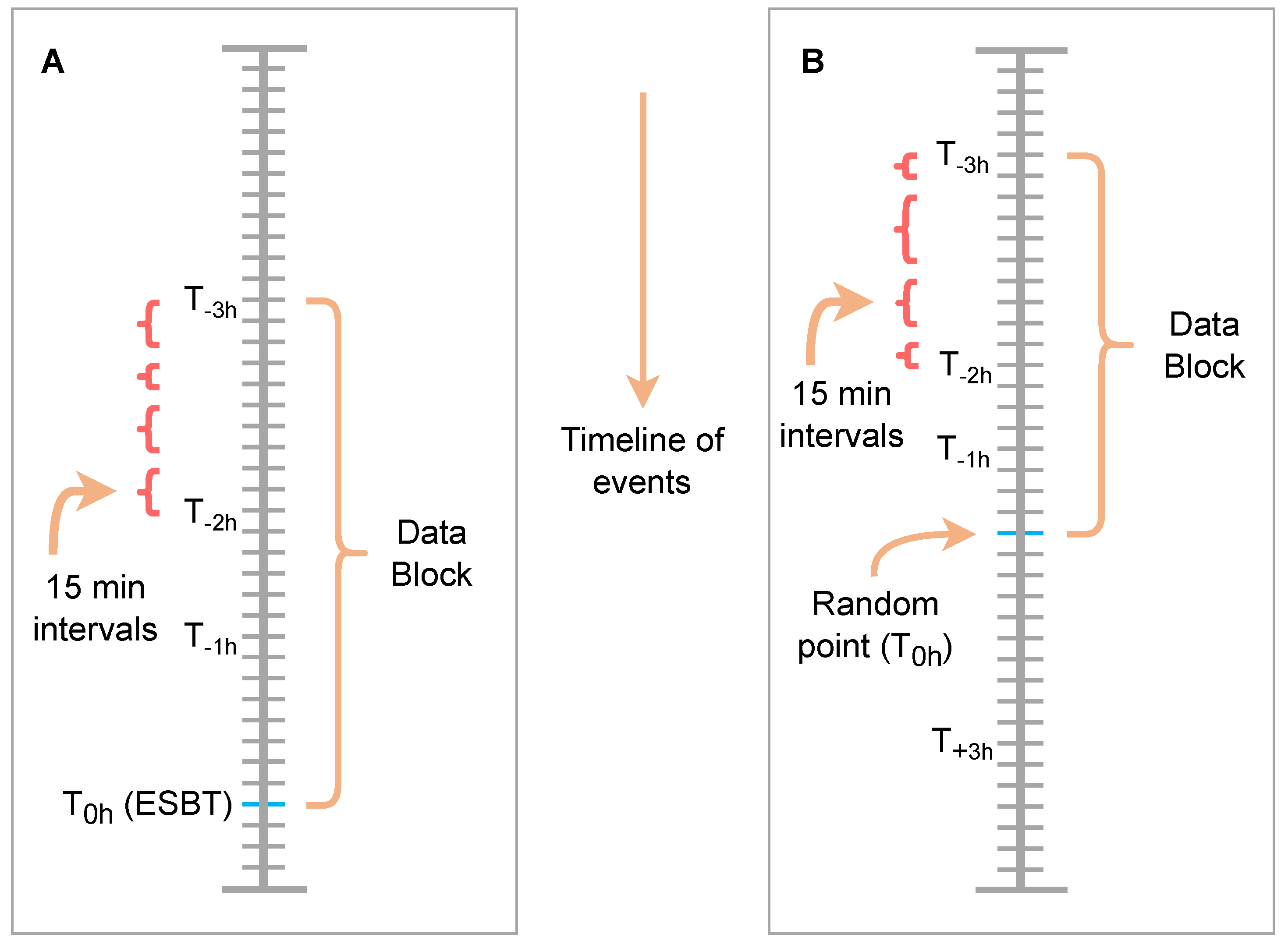
Figure 2A demonstrates this graphically. An ESBT event (blue) is shown and labelled
. From this point all data 3 h previous is filtered for (labelled
). This section of extracted data is referred to as a data block and is subsequently divided into 15 min intervals (red curly braces). Note, the number of data instance in these 15 min intervals is not uniform since the nature of event data is not to collect in a continuous manner. Provided no other ESBT event is found between
and
, the mean and the standard deviation (SD) of the features contained within each 15 min interval is calculated, resulting in 12 data instance (i.e., there are twelve 15 min intervals in a 3 h window). If a second ESBT event is found within the 3 h window, then only 15 min intervals between the first and second ESBT event are used to calculate the mean and standard deviation, resulting in fewer than 12 data instances. These generated instances containing the mean and standard deviation values of the available features are labelled as the positive examples and considered to represent an ESBT event.
2.2.2. Negative Examples
For this study, negative examples were considered to be those sections of the data whereby engine parameters were deemed to be under normal operation. Since positive examples were created from data immediately prior to an ESBT event, negative examples were therefore created from instances of data where an ESBT event is not found in the immediate vicinity.
Figure 2B graphically demonstrates the process undertaken. Data for a unique DMU engine is extracted as described previously. Within this expanse of data there are instances of ESBT events; however, for the majority of the data entries the engine is considered to be working satisfactorily. A random point in the timeline of the data is selected, labelled
, all the data ±3 h from this point is obtained. A check is made in this 6 h window (i.e., random point ±3 h) for any ESBT events. If an ESBT event is found, a new random point is selected and the process repeated until no ESBT event is found in the 6 h window. If no ESBT event is found, all the data between
and
(the data block) is taken and divided into 15 min intervals, and as previously described the mean and standard deviation is calculated for each interval. For each unique unit in the dataset an arbitrary value of 3 was chosen as the number of iterations processed before moving onto the next unit. These generated data instances containing the mean and standard deviation values of the available features are labelled as the negative examples and represent no occurrence of an ESBT event.
Figure 2.
Three hour windowing, to produce positive (A) and negative (B) binary examples from the event data.
Figure 2.
Three hour windowing, to produce positive (A) and negative (B) binary examples from the event data.
2.2.3. Feature Reduction and Balanced Dataset
The data preprocessing described above (see
Section 2.1), retained 39 features from the dataset, which were available during the generation of the binary examples (positive and negative examples). Since the positive and negative examples are generated independently, there may be occurrences whereby the resulting available features differ between the binary examples (this is a phenomenon analogous to the nature of the event data). To correct this, prior to collating the binary instances together, the intersection of the available features is taken. This process removes the disjunctive union of the features between the binary examples. During negative example processing (see
Section 2.2.2), selection of the random point,
, means that the features which contain entries around that random point will vary for each iteration. This can result in a different set of features being available for classification per iteration and therefore must be corrected post-processing.
Due to the nature of event data and limited number of ESBT failures in the dataset, the preprocessing described above generates many more negative examples than positive examples. Using these instances would result in an unbalanced dataset that would bias the training capability of the machine learning model and affect its ability to generalise. To address this, a random sample of the negative examples which equates to the number of available positive examples is taken. This produces a dataset that contains approximately an equal number of positive and negative examples, which can then be used for training and testing of classification models.
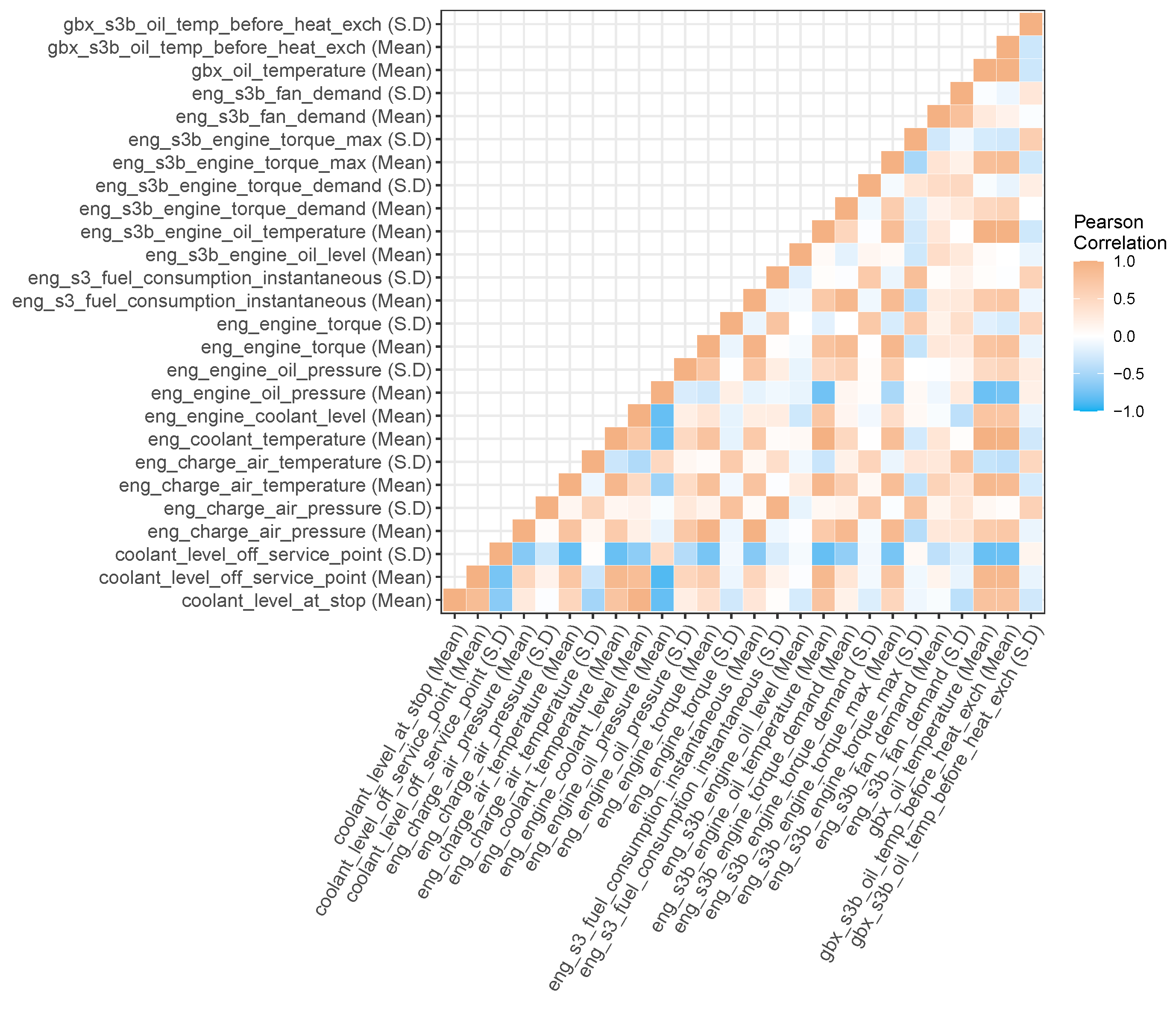
After concatenating the binary examples together, a final feature reduction step is undertaken. A low variance filter is applied to remove features that contain constant values. All but one of any two or more features that are highly correlated (Person’s correlation coefficient
) are removed using a linear correlation filter. An example of the correlating features for the 3 h windowing models (
h to 0 h) is shown in
Figure 3 as a heatmap. These are the features available prior to removal with the linear correlation filter.
Finally, features which contained more than 50% missing entries are removed, and data instances that contain a tuple of missing values are removed entirely. Removing tuples may unbalance the dataset to a small extent but observations during data processing showed this not to be of concern (see
Table 2).
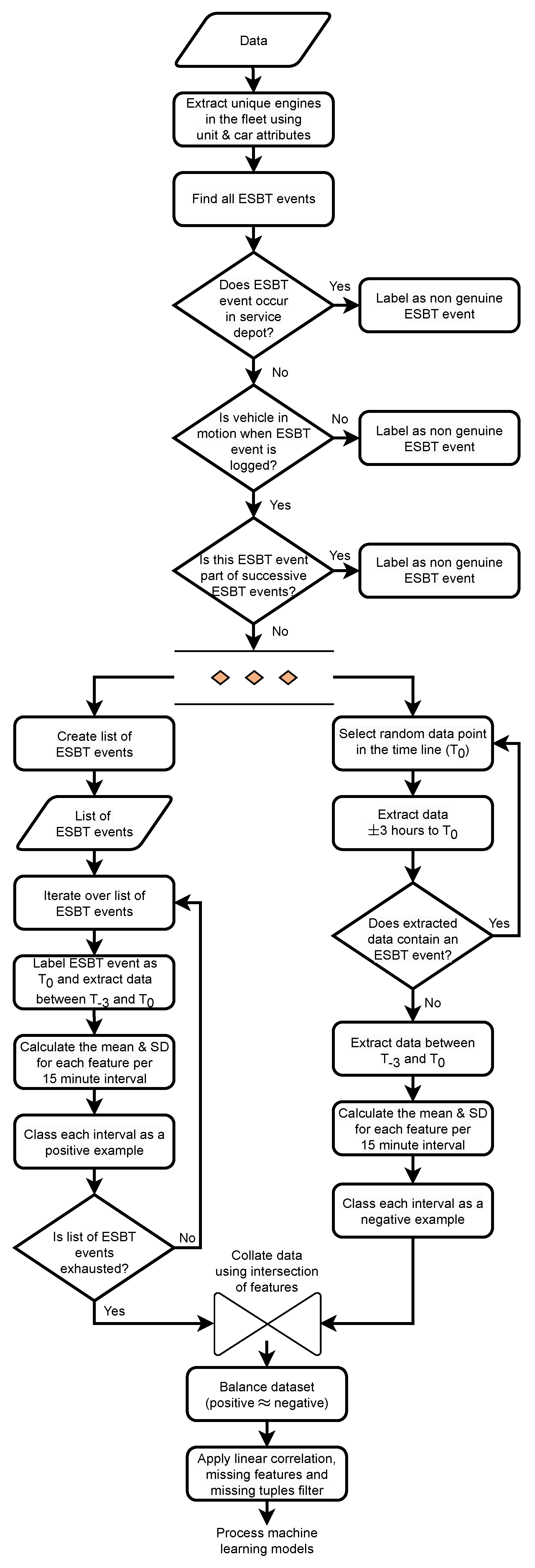
A workflow representation of the data preprocessing and generation of binary examples is demonstrated in
Figure 4. The methodology described, uses a 3 h window (data block) during the generation of binary examples. This 3 h window was chosen arbitrarily during the development of the methodology but in essence any window size could be chosen. To better understand the outcome of the machine learning models, we processed our data using several different window sizes (data block size) as shown in
Table 2.
3. Classification Models
In this study, two machine learning methods were used for the classification tasks; The C4.5 decision tree [
25] and random forest [
26], while both algorithms are robust to missing values, the decision tree is a useful surrogacy model that can assist in providing explainability for the random forest method.
The decision tree algorithm chooses attributes based on how effectively it can split the data into their respective classes. Attributes which demonstrate the highest normalised information gain become the split criterion at each level of the tree. C4.5 then repeats on the smaller subset until all the data are processed. Pruning was not used during decision tree training and the Gini index was chosen as the quality measure. Previous studies have reported that no significant difference is observed in decision tree outcome when using the Gini index compared to other popular methods such as Information gain [
27,
28].
The random forest is an ensemble method of many decision trees. An output prediction is based on the mode of the classes of each individual tree. A subset of the training set, known as the local set, is used to grow each individual tree, and the remaining samples are used to estimate the goodness of fit. The local set used to grow each tree is split at each node according to a random variable sampled independently from a subset of variables. 500 trees were chosen for the random forest models, with greater numbers showing no improvement in prediction.
To test the robustness of the models, 500 iterations of the decision tree and random forest models were trained and tested. For each iteration a new random 70:30 training:testing split was used.
Explainable Artificial Intelligence
Explainable Artificial Intelligence (XAI) methods are techniques and approaches that aim to provide explanations or justifications for the decisions made by AI models or systems [
29]. These methods play a crucial role in enhancing transparency, interpretability, and trustworthiness in AI systems, especially in complex and black-box models. They strive to explain how a model generates an output based on a given input.
The available XAI methods can be broadly categorised based on their functionality. For instance, model-specific methods [
30] are tailored for a specific type or class of algorithm, whereas model-agnostic methods [
31] can be applied to various machine-learning algorithms. Naturally, XAI methods are particularly popular for so-called “black box” machine learning algorithms like neural networks or random forests.
To gain insight into the outcomes of the random forest models, in this study three different model-agnostic XAI methods are used: Skater [
32], Sage [
33], and Shap [
31]. These methods are particularly effective for datasets of reasonable size as they eliminate the need for retraining separate models. However, it’s important to note that for extremely large datasets, some of these methods may encounter computational complexities that limit their applicability.
The aforementioned methods are classified as perturbation-based techniques since they perturb feature values to simulate the absence of a particular feature and estimate its contribution. The variation resulting from this perturbation affects any correlation between the perturbed feature and the target variable; ultimately determining the influence of the feature on the model’s predictions. Although all three methods employ perturbation, they differ in their computational approaches, such as the number of features permuted or the choice of loss function used to estimate the models’ performance.
These XAI methods can provide explanations at both the local and global levels. Local explanations [
34] offer insights into individual instances within the dataset, shedding light on the decision-making process for specific cases. On the other hand, global explanations [
32] provide explainability for the entire dataset, giving a comprehensive understanding of the model’s behaviour.
The Skater method employs a single feature perturbation to provide global explanations. It measures feature importance by using the cross entropy/F1 score. On the other hand, the Sage and Shap methods compute the mean average from multiple feature coalitions. They estimate feature importance using Shapley values [
35], which are derived from the Cooperative game theory approach. While Sage offers global explanations directly, the Shap method combines all the local explanations to generate a global interpretation of the model’s predictions.
For the processed data used in this study, it is desirable to have explanations that describe the model’s overall decision behaviour. Therefore, a global explanation is sought. This will help us understand how the features available to the random forest model influenced its predictions. It will also provide insight into the usefulness of the features originally selected for engine failure predictions from the unprocessed original dataset.
4. Results
Using the methodology discussed above, 500 iterations of the decision tree and random forest models were tested. Five different data blocks of various size ranging from 1 h up to 24 h were tested.
Table 2 shows the results of these models reported across the 500 iterations. The accuracy represents the mean value of the 500 iterations, while the True positive, False positive, True negative, and False negative values are the sums across the 500 iterations. These model statistics have been reported in other similar studies [
36] and were appropriate for this work.
For all the data blocks tested, the available features for the models does not change drastically, and all the models had between 15 and 17 features available during the training process. The features available are determined by the processing of the positive and negative examples as discussed in
Section 2. As the data block size increases, so does the number of instances in the final dataset prior to machine learning. The class imbalance between the positive and negative examples for all the models tested does not differ by more than 7% (
h to 0 h; 139/150 class split) and therefore the imbalanced dataset problem was not of concern here.
Random forest models outperform the decision tree models, based on their accuracy and F1 scores. This is somewhat expected since the random forest is an ensemble method made up of many decision trees which helps reduce overfitting of the data [
26]. This becomes more pertinent when training dataset sizes are small. With respect to the data block sizes tested, the
h to 0 h produces the best model results for both the decision tree and random forest models with an accuracy of 83 and 88%, respectively. These models also produce the highest F1 scores of 75 and 81% for the decision tree and random forest models, respectively. The F1 score (2 × (Precision × Recall)/(Precision + Recall)) is preferable when working with imbalanced datasets (note, the precision and recall metrics are discussed below). This metric considers the prediction errors your model makes as well as the type of errors that are made. Given the high scores achieved, suggests any class imbalance issues were not present. Collectively, these results suggest the 5 h window used to extract data from (see
Section 2) contains the most signal for engine failures. A data block window size much smaller (i.e.,
h to 0 h or
h to 0 h) does not contain enough information to discriminate between the positive and negative examples, while a window size much larger (i.e.,
h to 0 h or
h to 0 h) will contain the necessary information but it is likely masked or diluted by the other data contained in the larger window size. The larger window size models tested are therefore less able to discriminate between the positive and negative examples in these cases. This provides some indication as to how far forward engine failures can be reliably predicted.
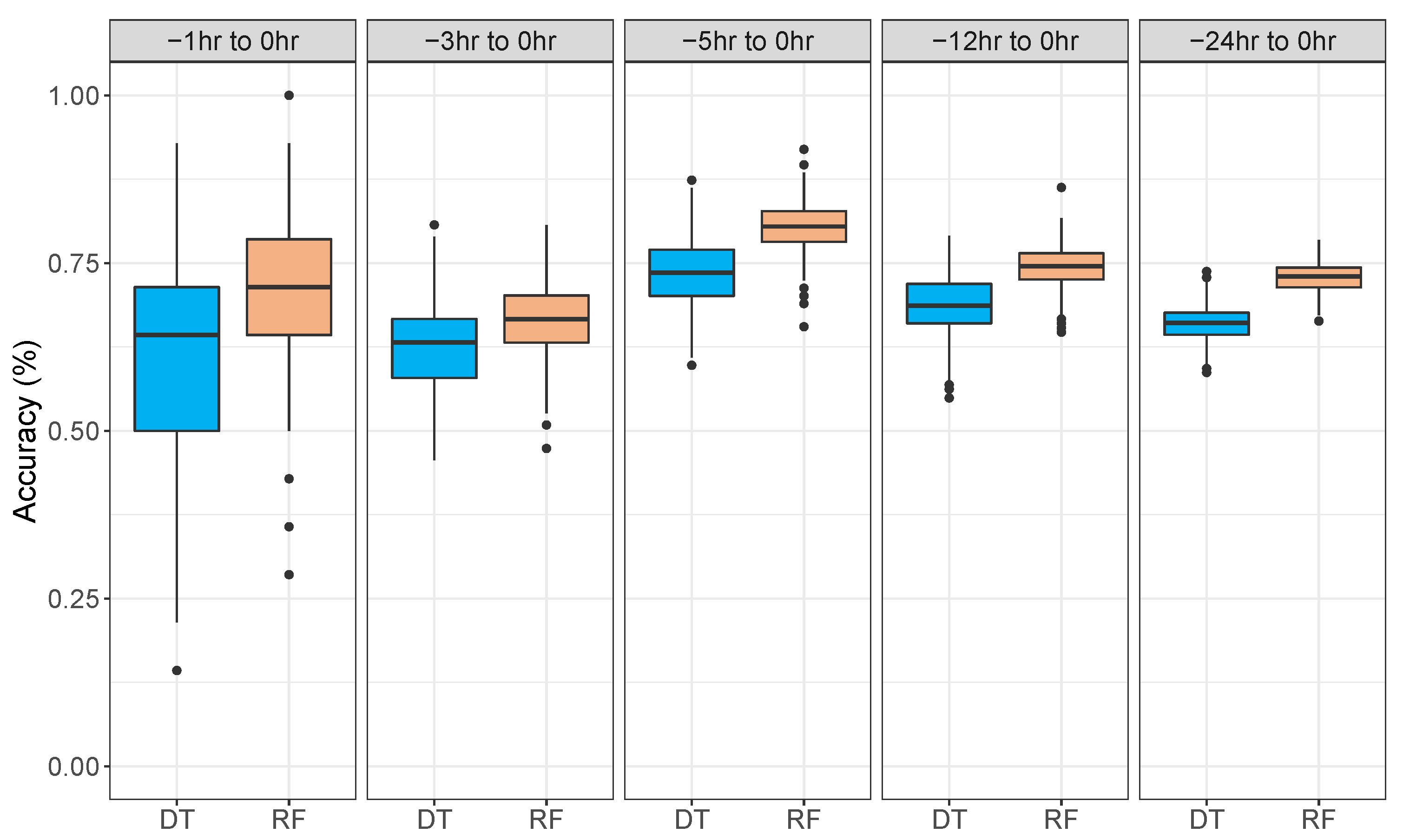
Figure 5 plots the accuracies of the 500 iterations as boxplots for each of the different data blocks tested in this study. From these plots, we can see the variability across the 500 iterations that were tested. The smaller data block size models (
h to 0 h) produce the largest spread in terms of distribution of accuracies, suggesting that at this data processing level, the models are highly variable. These models produced the largest standard deviation values across the 500 iterations of 0.13 and 0.11 for decision tree and random forest models, respectively. As the data block sizes increase (hence more data instances available for training and testing) the standard deviation across the 500 iterations of the models gets smaller. With more data, the robustness of the models in terms of precision is much better. The best-performing models (
h to 0 h) have standard deviations of 0.05 and 0.04 for the decision tree and random forest models, respectively.
The True positive, False Positive, True Negative, and False Negative columns of
Table 2 show the confusion matrix of the models, summed across the 500 iterations. From this information we are able to calculate the precision and recall values of the models. These measures help evaluate the performance of a classification model. The precision (True positive/(True positive + False positive)) establishes what proportion of the positive predictions are actually correct, i.e., what proportion of engine failures were accurately predicted. The recall (True positive/(True positive + False negative)) measures the proportion of actual positives that were predicted correctly [
37,
38]. Again, the
h to 0 h models produce the best precision and recall values of all the models. The decision tree models resulted in a precision value of 0.74 and a recall value of 0.77. The random forest models produced a precision value of 0.80 and a recall value of 0.83. High precision and recall values are desirable [
38] although there may be a trade-off between the two measures. Although the methodology described in this work involves balancing the dataset with positive and negative examples, in reality there are far fewer positive examples than negative ones. The ability of a classifier to discriminate the positive examples is important and a strong precision value is indicative of that. Precision and recall values for the other models were also encouraging and demonstrate the strong predictive performance of the classifiers (values not reported).
To better understand how the decision tree models made their choices the tree data across all 500 iterations was extracted for the best performing model (
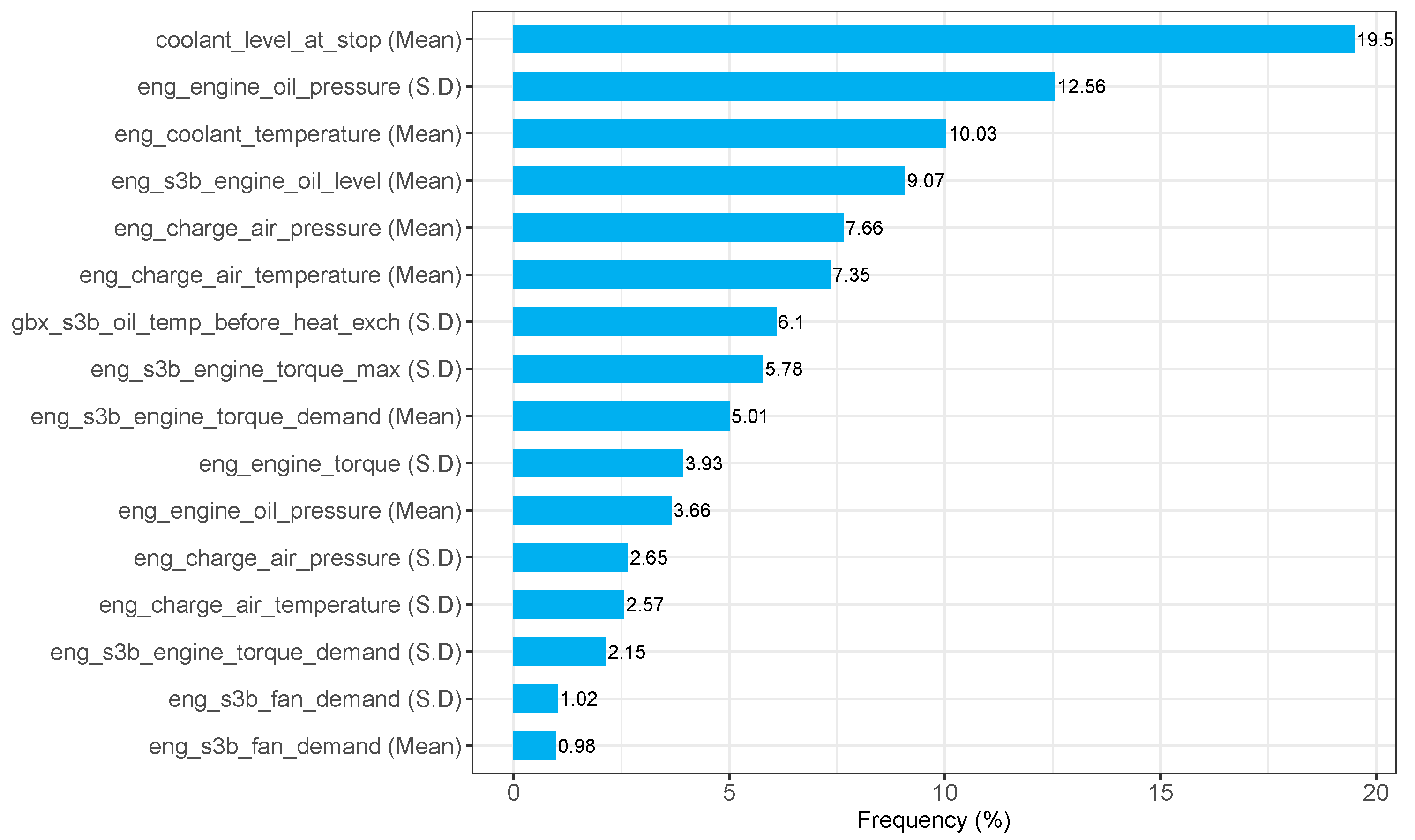
h to 0 h). Features used at the split criterion for each node of every decision tree was extracted. A frequency count of the features used was turned into a percentage value.
Figure 6 plots this data graphically as a bar chart. The
h to 0 h models had 17 features available for the training process of the decision tree models (see
Table 2). Of those 17 features only 16 were actively used (see
Figure 6). Three of the features were used by the models 10% or more times of the total usage. These features were related to the coolant level of the engine (coolant_level_at_stop (Mean) and eng_coolant_temperature (Mean)) and the oil pressure of the engine (eng_engine_oil_pressure (S.D)). The remaining 13 features were used across the 500 iterations a total of less than 10% of the time. This information provides some insight into the features that are actively used by the decision tree models to base their decisions on. A frequency count of the features used shows how often the decision tree relies on those features at each split criterion in the decision tree, providing some insight into the usefulness of the features.
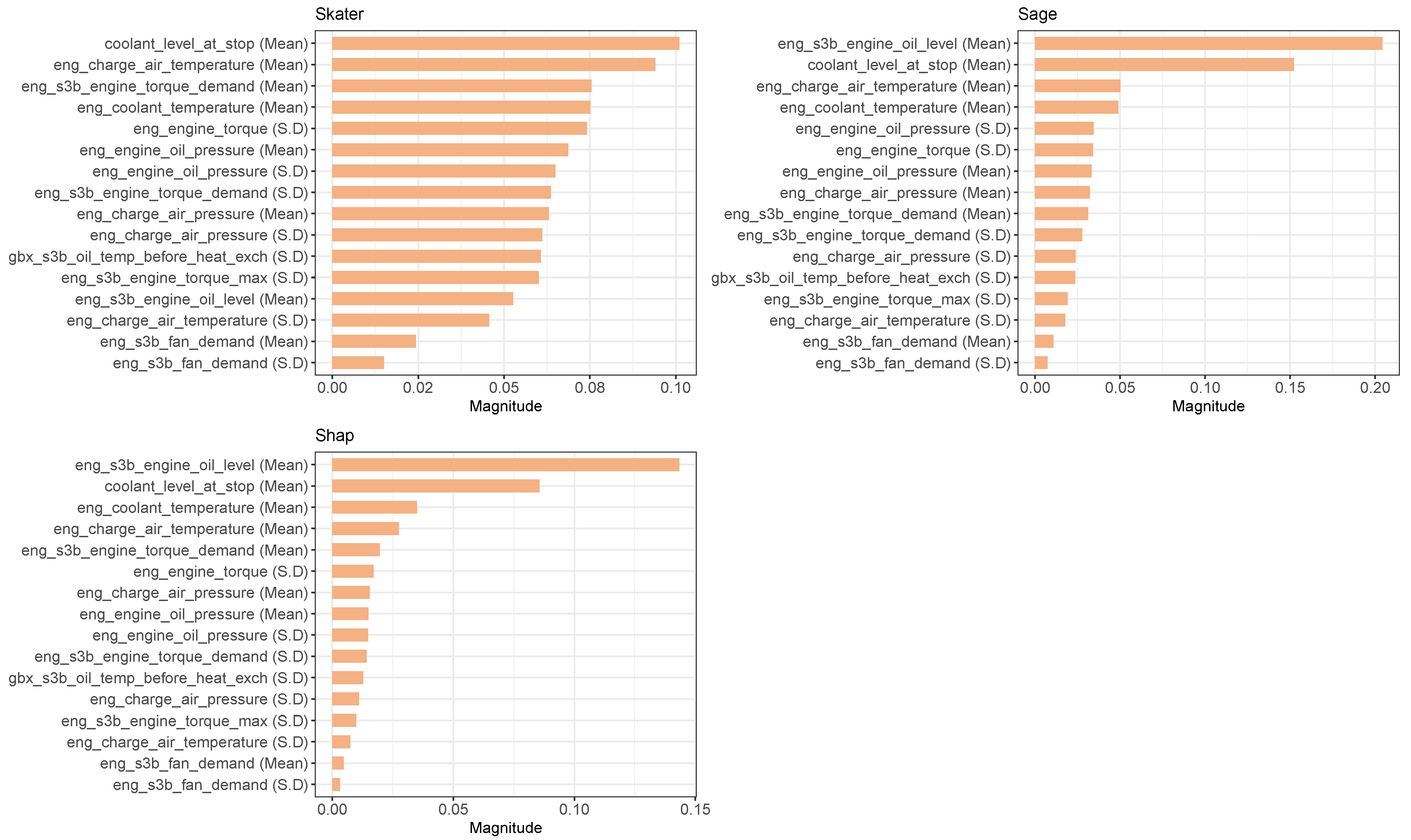
To provide some element of explainability for the random forest models, three different XAI methods were tested on the best performing models (
h to 0 h). Random forest models trained and tested on data from the
h to 0 h data block window were run alongside each XAI method.
Figure 7 plots the magnitude values calculated by each of these methods for each of the features available to the random forest model. As with the decision tree models, the random forest models only used 16 of the 17 features available to them. The significance of these features on the model’s predictive power is given by the magnitude calculated by the Skater, Sage, and Shap methods (see
Figure 7). The greater the magnitude the greater the effect of that feature on the model’s outcome. Although the different XAI methods produce slightly different results, due to the way they calculate feature importance, there are some commonalities, which are useful for explaining the random forest models’ decisions. For instance, when considering the top five features with the greatest magnitudes for each of the XAI methods, we find that three of the features are common between them; “coolant_level_at_stop (Mean)”, “eng_charge_air_temperature (Mean)”, and “eng_coolant_temperature (Mean)”. Two of these three features (“coolant_level_at_stop (Mean)” and “eng_coolant_temperature (Mean)”) were also used 10% or more times by the decision tree models. The XAI methods also demonstrate which features are least important in the model’s predictive outcome. For all the XAI methods used, the same three features appear as the least important features and in the same order. These are; eng_charge_air_temperature (S.D), “eng_s3b_fan_demand (Mean)”, and “eng_s3b_fan_demand (S.D)”.
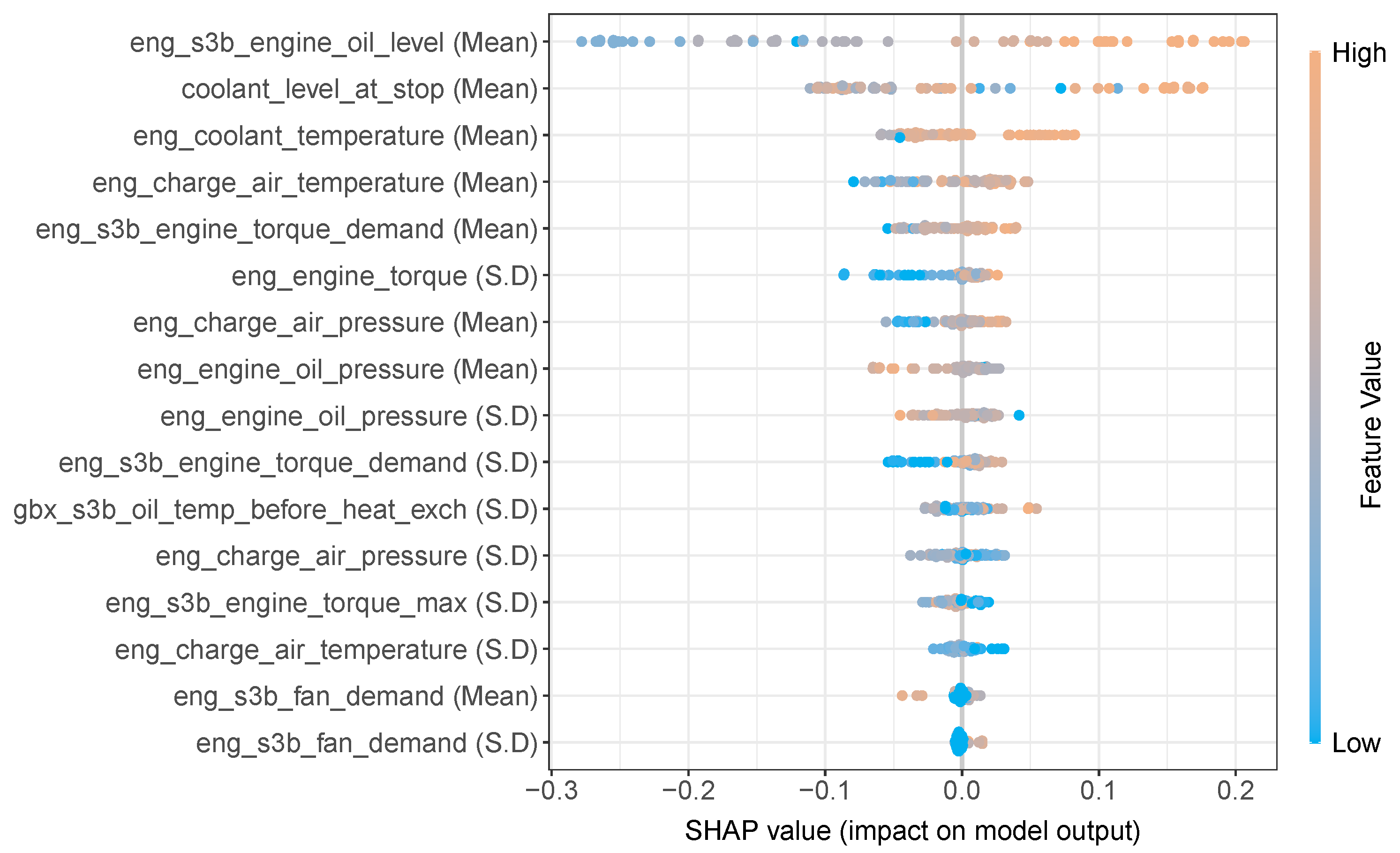
The outcome of the Shap XAI analysis can be further examined by means of a Shap summary plot as shown in
Figure 8 below. The Shap summary plot shows the features available to the random forest model on the
y-axis and lists them in order of importance. The Shap value assigned to each instance in the test set are represented by the
x-axis and the gradient colour represents the original value for that feature. Note, that each feature in the data was of a continuous numerical type. Each point on the plot represents an instance of the test set. The feature which resulted in the largest magnitude using the Shap XAI method (see
Figure 7) was the “eng_s3b_engine_oil_level (Mean)”. The Shap summary plot shows this feature at the top of the plot, also indicating it to be the most important. It additionally shows instances of this feature which have a “high” value, predominantly prompts the random forest model towards a positive (ESBT) prediction, which is reflected by the positive Shap value. Similarly, for the same feature, a “low” value, predominantly prompts the random forest model towards a negative outcome (non EBT), which is reflected by a negative Shap value. Likewise the feature “eng_engine_oil_pressure (Mean)” is the eighth most important feature, but shows that a “low” value for this feature generally results in positive Shap value which prompts the random forest towards a positive prediction (ESBT) and conversely a “high” value for this feature generally results in a negative Shap value which prompts the random forest towards a negative prediction (non-ESBT).
5. Discussion
In this study, a methodology capable of processing sparse event data for classification modelling is proposed. Large volumes of real-world sensor data taken from a fleet of diesel multiple units are processed to demonstrate how highly predictive machine learning models can be trained. The best models resulted in high predictive accuracies of 83% and 88% for decision trees and random forests, respectively, suggesting the windowing method of processing the event data is a pragmatic choice. The proposed method takes unclassified event data and produces classified examples that are used for machine learning classification tasks. The event data used in this work was time-stamped, and therefore various data block sizes could be processed as discussed in
Section 2.
Processing the data using various data block window sizes helped identify the optimal window size that produced the most accurate models. As the data block window became larger from 1 h (
h to 0 h) up to 5 h (
h to 0 h) the accuracy of the models improved, suggesting the strongest signal for engine failure in the data appears to be contained within a 5 h window of the actual ESBT event. For this work specifically, the
h to 0 h data block window repeatedly produced well-trained accurate models (across 500 iterations). Smaller window sizes produced less accurate models, most likely due to the limited data available to train the models. Other studies in the literature, however, have successfully used low data volumes for predictive maintenance tasks [
17]. Model accuracies were most variable at the
h to 0 h data block size, and improved as the data block sizes became larger. Once the data block window exceeded the 5 h size, a drop in the accuracies was observed (see
Figure 5 and
Table 2).
The initial data curation of this study involved the manual selection of features deemed relevant to engine failures (see
Section 2). A total of 39 features were selected which were further reduced through subsequent processing steps. The best performing models (
h to 0 h) had 17 features available during model training. Understanding which features are important for a model’s decisions provides some useful insight into which features are relevant for predicting engine failures. The resulting tree structures for the best performing decision tree models (
h to 0 h) were analysed. Features relating to coolant level, oil pressure and coolant temperature (see
Figure 6) were frequently used across the 500 iterations of the decision trees. Similarly, three different XAI methods showed that the random forest models heavily relied on features pertaining to coolant level, coolant temperature, and engine air temperature as prominent features of importance, while XAI methods are useful, they can produce a slight difference in results as shown in this study (see
Figure 7). Studies have attempted to consolidate the outputs of various XAI methods with varying degrees of success [
39]. Furthermore, for the Shap XAI method, the influence each value of a feature has towards a positive or negative prediction can be visualised using the Shap summary plot (see
Figure 8). Such information helps provide explainability behind a model’s performance.
The authors understand potential caveats in the work pipeline may exist and are discussed herein. The dataset used in this study spanned the period of 1 year (October 2019 to October 2020). Although the volume of data was considerable (approx 14 M records), the number of ESBT events in the dataset is infrequent. To circumvent issues of bias data the methodology proposed equating the ESTB events (positive examples) with non-ESTB events (negative examples). This ensured the data are not massively imbalanced prior to model training. In practice, live data would likely be imbalanced and is a consideration to take into account if deploying these models. A suggested solution could be to train the models on a balanced dataset, ideally on more than 1 years worth of data, before deploying into the real world. Using collected data that covers a longer period, means the models can be trained with more certainty.
Since the event data was time-based, larger window (data block) sizes produced more data to train and test the models on. For this study, the largest window size went as far back as 24 h ( h to 0 h models), but all the data block sizes tested, had their end point at the ESBT event (0 h). This was a constraint of the study due to the nature of the data that was used. In an ideal situation, the data block window that is processed should be a window as far back on the timeline from the ESBT event as possible. For instance, if the ESBT event is denoted on the time line (i.e., 0 h) then an ideal 3 h data block window could be taken from to . This can be interpreted as a data block window of 3 h in size, taken from the event data time line, between 12 h and 9 h prior to an ESBT event. This would be the preferred way to process the data and will be explored in our future work. The limitation of the work in this study utilises data of different window sizes immediately prior to the ESBT event. Additionally, to gain maximum benefit from a predictive tool it would be useful to have a longer warning period for a potential engine failure. Future work will also consider how far in advance it is possible to predict a likely engine failure based on this type of event based data.
This study chose to focus on features thought to affect engine failure, these were features related to the engine, gearbox, battery and vehicle speed. In essence there may be other features in the dataset that could be useful but were removed at the processing stage (see
Section 2.1). These features could be explored as part of the processing and may enhance the findings of this study.
The data sample size used in this study covered a period of one year. To corroborate the models usefulness, it would be beneficial to use additional data as an external validation set. This is a common practice in the domain of machine learning, but for this study additional data was not available. It may have been possible to partition the data that was available prior to any processing and hold back a sample as the external validation set. However, this approach was not explored since the occurrences of ESBT events in the data are few. Using all the data, therefore, ensured the models learned from as many diverse examples as possible.


