Logistic Model Tree Forest for Steel Plates Faults Prediction

Abstract

Fault prediction is a vital task to decrease the costs of equipment maintenance and repair, as well as to improve the quality level of products and production efficiency. Steel plates fault prediction is a significant materials science problem that contributes to avoiding the progress of abnormal events. The goal of this study is to precisely classify the surface defects in stainless steel plates during industrial production. In this paper, a new machine learning approach, entitled logistic model tree (LMT) forest, is proposed since the ensemble of classifiers generally perform better than a single classifier. The proposed method uses the edited nearest neighbor (ENN) technique since the target class distribution in fault prediction problems reveals an imbalanced dataset and the dataset may contain noise. In the experiment that was conducted on a real-world dataset, the LMT forest method demonstrated its superiority over the random forest method in terms of accuracy. Additionally, the presented method achieved higher accuracy (86.655%) than the state-of-the-art methods on the same dataset.

1. Introduction

A fault is defined as an unexpected, abnormal, and undesirable situation, behavior, or imperfection at the equipment, component, or sub-system level which may cause a failure. Faults influence the wear and corrosion resistance of the product, reduce the production quality, and produce non-usable materials in the worst case. Such a physical malfunction can lead to unavoidable crashes and stop the system from working properly. Fault prediction is the process of identifying fault-prone components related to specific domains based on predictive analytics. In other words, it predicts different deviations in materials from their expected or normal states. Determining fault types in an effective way can reduce unexpected waste, maintenance, repair, or replacement costs, as well as improve the quality level of products and production efficiency. Fault prediction leads to extend equipment lifetime and asset utilization in various industrial environments. Moreover, it avoids long-term decline in total profits of the related system and also the outflow of customer confidence. The higher level of quality a product requires, the better fault prediction technique the industries should develop. In this context, intelligent systems, derived from research on machine learning, have been established to handle this issue correctly and quickly.

The steel industry has been shown to be one of the primary industries that requires fault prediction to produce materials in the most meticulous way. From making machines to beautiful artworks, steel plates are commonly used in a diverse range of applications, namely in industrial machinery, building construction, automobile chassis construction, bridge structures, and shipbuilding. Having such widespread applications, high-accuracy control of steel plate surfaces is important for meeting strict quality requirements. However, the difficulty of flat steel sheet manufacturing has always been considered in the industry because of the deformation tendency which is often caused by the steel surface coming in contact with different machines in manufacturing steps such as casting, drawing, pressing, cutting, and folding. Consequently, this study aims to recognize the types of defects that steel plates have. One of the traditional ways is the manual inspection of steel plates by human experts to detect defects. However, this practice is very time-consuming, inaccurate, and costly, which needs considerably more human effort and overlooked investigation. Therefore, automation of fault prediction is necessary to reduce costs and minimize the time needed for monitoring. Here, machine learning plays an important role by analyzing past data to find hidden patterns and then construct models to predict the faults. Machine learning-based fault prediction methods contribute to facilitating precautionary maintenance and avoiding quality problems of the materials by more accurate and efficient decisions.

Machine learning (ML) draws inferences to predict future outcomes by finding patterns from historic data. It provides computers with the ability to learn by utilizing different algorithms and makes predictive models for artificial intelligent-enabled systems. As one of the ML methods, the logistic model tree (LMT) [1] is a decision tree-based model, which fits the logistic regression learning algorithm. The competitive advantages of LMT are the efficient construction and the simplicity of its interpretation. LMT builds a single compact tree by means of effective pruning mechanisms. In addition, the key features of the LMT algorithm include working with numeric and binary values, nominal qualities, numeric variables, and missing data, which all provide it with the information to achieve the best result in many studies [2,3,4,5,6,7].

Although LMT usually provides high classification performance and strong generalization ability [8,9,10,11,12,13,14,15,16,17,18,19], building a single tree classifier may not be enough and may lead to less accurate predictions. On the other hand, in ensemble learning, the weakness of a classifier can be overcome by the strengths of other classifiers. Although several classifiers in the ensemble produce incorrect outputs, other classifiers may have the ability to correct those errors. Therefore, in the current study, we present a novel ensemble method that builds many LMT trees and combines them together to make a final prediction.

The main problem faced by researchers when doing steel fault prediction with machine learning is the imbalanced and noisy data. In practice, the distribution of fault types is usually imbalanced, which means that the number of observations of a class is extremely high when compared to another class in a dataset. Imbalanced data makes the machine learning model seriously biased toward the majority class, thereby degrading the performance of it on the minority class. In this study, our method provides a way to prevent class imbalance and eliminate noise samples by using the edited nearest neighbor (ENN) technique.

The novelty and main contributions of this study are summarized below:

(i)

This article proposes a new ensemble technique, entitled the logistic model tree forest (LMT forest).

(ii)

Our work is original in the literature since it contributes to building decision trees based on the LMT method to construct a forest for steel plate fault prediction.

(iii)

The study is also original in that it applies the edited nearest neighbor under-sampling approach to the dataset before detecting steel plate faults.

(iv)

In the experiments, the proposed LMT forest method with an accuracy of 86.655% outperformed the random forest method with an accuracy of 79.547% on the same dataset.

(v)

Our method achieved higher classification accuracy than the state-of-the-art methods [20,21,22,23,24,25,26,27,28,29,30,31,32] on the same steel plate fault dataset and demonstrated its superiority over its counterparts.

The rest of the current paper is arranged as follows. The related works are explained in Section 2. The proposed LMT forest method is described in detail in Section 3. The experiment results are provided in Section 4. Finally, the study is condensed and some future works are suggested in Section 5.

2. Related Works

In the literature, common mechanical components that have been considered in fault prediction systems include the bearing [33], gearbox [34], belt-pulley [35], shaft [36], and induction motors [37] (i.e., stator and rotor). Moreover, surface defect prediction from different aspects, i.e., texture, color, and shape features, is possible in industrial products based on machine learning techniques [38]. Fault prediction is applied in different areas such as manufacturing [39,40,41], health [42], transportation [43], seismology [44], power systems [45], telecommunication networks [46], chemistry [47], electrical machines [48,49], energy [50], and environmental work [51]. In this study, fault prediction is applied to the manufacturing process, in which the accurate investigation of products is essentially considered to reduce processing cost and time, and improve product design and quality.

2.1. Machine Learning-Based Fault Prediction

Machine learning-based fault prediction has been investigated with real-time monitoring in manufacturing environments. In [52], random forest (RF) classification was employed for the prediction of input data issues, and the NoSQL MongoDB as a big data technique was applied to the collected environmental dataset from the Internet of Things (IoT) sensors in an automotive manufacturing production line. Moreover, blockchain technology was utilized for covering system security. In another work [53], the utilization of machine learning models in the battery management system of a lithium-ion battery for the prediction of faults in the remaining useful life (RUL), charge state, and health state were presented by means of a neural network (NN) with a support vector machine (SVM), genetic algorithm back propagation neural network (GA-BPNN), RF, Gaussian process regression (GPR), logistic regression (LR), and long short-term memory recurrent neural network (LSTM-RNN). In another study [54], the authors focused on a bearing fault prediction method for electric motors by applying a medium Gaussian support vector machine (MG-SVM) on a motor bearing dataset.

The application of deep learning methods to predict faults has been investigated in various studies [55,56,57,58]. In [55], a fault prediction workflow by deep learning for seismic data was developed, in which convolutional neural networks (CNNs) for image recognition, U-Net architecture for image segmentation, random forest for identifying the most important attributes, and GANs-based reconstruction approach for clarifying fault locations were used on the seismic data. As a result, the highest importance for the “discontinuity along dip” feature among seismic attributes was specified, and the prediction accuracy of fault probability maps was improved. Similarly, in another work [56], the authors proposed a structure-based data augmentation framework to boost the variety of the semi-real-semi-synthetic seismic dataset collected from various work areas in the Tarim Basin of China for improving fault prediction and identification on the basis of deep neural networks and U-Net, respectively. In another work [57], fault prediction and cause identification approaches based on deep learning in complex industrial processes were reported. The authors utilized deep learning to predict the fault events, long short-term memory (LSTM) to adapt to the branch structures, and an attention mechanism algorithm for fault detection and cause identification on the sensor-based data in a production line considering various fault types. Yang and Kim [58] detected recurrent and accumulative fault situations and calculated the anomaly scores in the data by using the LSTM method.

Fault prediction in wind turbines has been investigated in previous studies [59,60] since it is a critical issue for maintaining the reliability and safety of energy systems. In [59], a novel solution for predictive maintenance in the generator of wind turbines was developed by means of supervisory control and data acquisition (SCADA) systems to control the state of operations in generators. Principal component analysis (PCA), SVM, NN, K-nearest neighbors (KNN), and naive Bayes (NB) classifiers were used to discriminate the various statuses of wind turbine generators. The synthetic minority oversampling technique (SMOTE) technique was applied to manage the imbalanced dataset for the wind power plants consisting of numerous wind turbines located in China. Low deployment costs were considered in the presented work by diagnosing the specific type of generator faults with high accuracies. In another study [60], the authors focused on a stacking gearbox fault prediction model for wind turbines on the basis of the SCADA data for wind turbines in a wind farm. The applied main techniques were recursive feature elimination (RFE) for selecting appropriate features, and RF, extreme gradient boosting (XGBoost), and gradient boosting decision tree (GBDT) for describing the usual circumstances of the wind turbines. The results revealed that RF, GBDT, and XGBoost approaches outperformed KNN, SVM, decision tree (DT), and AdaBoost according to the high R² scores, and the low mean absolute error (MAE) and root mean square error (RMSE) metrics for various turbine types.

Wan et al. [61] presented a model based on the Dempster–Shafer (DS) evidence theory and a quantum particle swarm optimization back-propagation (QPSO-BP) neural network for the prediction of rolling bearing faults types under different operation conditions. They found the optimal initial weights and thresholds of the neural network. The authors used a rolling bearing dataset and achieved high-performance accuracy with the presented method in comparison to SVM-DS, DT-DS, RF-DS, KNN-DS, and K-means-DS regarding the macro area under curve (AUC) metric.

Yang and Li [62] developed a fault prediction method for wind energy conversion systems to improve the performance of the fault prediction model, shorten the time of fault prediction, and reduce the deviation between the actual fault value and the fault prediction value. The outperformance of the presented method was proved based on the kurtosis factor in comparison with the revealed results for fault prediction in different wind energy conversion systems. In the other work [63], the performances of various machine learning approaches were reported for forecasting heating appliance failures with the aim of predictive maintenance. In the mentioned work, the necessary data were collected from installed sensors of boiler appliances in homes. The results indicated that the LSTM models achieved higher accuracy than DT, NN, and weighted NN models based on different metrics for no fault, light fault, and severe fault states. In the other study [64], a smart machinery monitoring system based on machine learning was implemented to simulate the operating state of machinery for fault detection with a reduced volume of transmission information in an industrial IoT. The obtained accuracy from the non-linear SVM algorithm was higher than the results of the NB, RF, DT, KNN, and AdaBoost algorithms.

Syafrudin et al. [65] introduced a hybrid prediction model which includes a real-time monitoring system for automotive manufacturing on the basis of IoT sensors and big data processing. Various approaches, namely Apache Storm as a real-time processing engine, Apache Kafka as a message queue, MongoDB for storage of the sensor data, density-based spatial clustering of applications with noise (DBSCAN) for outlier detection, and RF classification for removing outliers were used in the mentioned study. In the other study [66], a fault prediction method was proposed to accelerate the speed of alarm processing and to improve the accuracy in the energy management system of microgrids via online monitoring, failure prejudging, and optimized SVM analysis. Early warning time and the high success rate of the proposed method were the consequences of their study. In another work [67], fault prediction of the in-orbit spacecraft was investigated based on deep machine learning and the massive telemetry and fault data. The algorithms such as least squares support vector regression (LS-SVR), auto-regressive integrated moving average (ARIMA), and Wavelet NN were utilized to determine the best model regarding normalized mean square error (NMSE).

Haneef and Venkataraman [68] employed LSTM, RNN, and a computation memory and power (CRP) rule-based network policy for predicting fog device faults. They collected related data by running the Internet of Things applications on different fog nodes. Their proposed method outperformed the traditional LSTM, SVM, and LR methods in terms of improved accuracy, lower processing time, minimal delay, and faster fault prediction rates. In the other work [69], the authors developed a machine learning-enabled method for fault prediction in centrifugal pumps in the gas and oil industry through multi-layer perceptron (MLP) and SVM techniques. They gathered the related data from the process and equipment sensors of centrifugal pumps to generate fault prediction alerts properly in decision support systems for operatives. In another study [70], the authors reported a fault prediction model with the aim of real-time tracking of sensor data in an IoT-enabled cloud environment for a hospital by machine learning. They applied the DT, KNN, NB, and RF techniques for controlling unanticipated losses produced by different faults. In another work [71], a real-time fault prediction recommendation model was developed by machine learning for a sensor-based smart office environment by means of a fault dataset retrieved from the sensors of office appliances. In their study, KNN, DT, NB, and RF were compared, and as a result, the RF algorithm revealed the highest accuracy against the others.

2.2. Steel Plate Fault Prediction

In this study, we focused on steel plate fault prediction, which is an active field of research in the science of metals because of its contribution to conquering the challenges faced in industrial manufacturing. Here, fault prediction can aid in quickly determining defects in products and then avoiding the probable costs. The process of detecting faults can be conducted by human experts, which is not obviously suggested in the current era of Industry 4.0. Such a time-consuming process may lead to imprecise decisions in material production. On the other hand, the other way is the utilization of specific types of machinery instead of human resources to capture faults in steel plates. If these faults are not predicted early in the manufacturing process, undesired effects, namely product failure and non-available materials, are highly probable. Therefore, it is essential to obtain hidden patterns in related data and consequently make an accurate prediction for steel plate faults. To achieve this objective, different machine learning techniques have been used in previous works, including support vector machines [20,25,29,30], neural networks [25,28,29], decision trees [20,21,24,26], naive Bayes [24,27], K-nearest neighbors [24,26,27], random forest [21,25,26,30,31], and AdaBoost [26,31,32]. In addition, deep learning approaches have been utilized, including long short-term memory [21] and convolutional neural networks [72]. Different from these previous studies, a logistic-model-tree-based solution is proposed in this paper.

2.3. The Application of the LMT Algorithm

LMT is a classification algorithm in the machine learning field that uses decision tree and logistic regression approaches to build a classifier as a special tree by taking advantage of both tree and regression concepts. In other words, it builds a tree with a logistic regression model at the nodes. LMT has been considered as an effective alternative for decision tree-enabled machine learning algorithms. The major benefits of LMT include working with numeric and binary values, nominal qualities, numeric variables, and missing data. In addition, LMT avoids data overfitting as a result of regression and classification techniques. Despite the advantages of LMT, building a single tree classifier may not be enough and may lead to less accuracy in the prediction. Therefore, in the current work, we present an ensemble method, the logistic model tree forest, which builds many LMT trees and combines them together to make a final prediction.

LMT has been applied in various fields such as health [5,6,14,15,17,18], forensic science [19], environmental work [7], earthquake [3,8], agriculture [13], and transportation [16]. For example, in [11], flash flood susceptibility maps were analyzed by the use of different machine learning algorithms, including LMT, multinomial NB, radial basis function classifier (RBFC), and kernel LR for solving the flood problem in Vietnam. The dataset consisted of flash flood features such as river density, land use, flow direction, and so on. The validity of the methods was measured regarding AUC and the best performance achieved by the LMT algorithm among the others. Their work was suggested for flash flood management by relying on the high accuracy of the model to specify flood-susceptible fields.

LMT was regarded as the best method among their counterparts in many studies [2,3,4,5,6,7,8,9,10,11,12,13,14,15,16,17,18,19,73,74]. For example, in [9], a susceptible landslide detection model in the Cameron highlands of Malaysia was reported, in which RF, LR, and LTM algorithms were applied to various databases such as soil maps, digital elevation models, geological maps, and satellite imagery. The results revealed the superiority of LMT over LR and RF based on the AUC metric. In the other study [10], the authors constructed a trustworthy map of shallow landslide susceptibility for Bijar City in Iran by different machine learning algorithms, including LR, LMT, NB, SVM, and NN. The reliability of the models was tested according to various metrics (i.e., MAE, RMSE). The outperformance of LMT was proved in comparison with other mentioned algorithms. Thus, the authors recommended the utilization of LMT in shallow landslide phenomena to reduce the related damages.

The LMT algorithm has been used in various studies to suggest solutions for machine learning-based problems due to its high accuracy in terms of different evaluation metrics. For example, in [13], the biochemical features of oil palm plants were monitored by using the spectroradiometer, machine learning, SMOTE, and unmanned aerial vehicle (UAV) techniques. In addition, three types of imbalanced datasets (leaf-raw band, canopy-VI, and canopy-raw band) were utilized to analyze nutrients in plants optimally and ensure their health and harvest. The outperformance of the LMT-SMOTEBoost was reported among alternative ones. In another work [14], LMT was applied to the medical field to predict miRNA-disease association (LMTRDA) by combining various information such as miRNA functional similarity, miRNA sequences, disease semantic similarity, and known miRNA-disease associations. Their model achieved a high accuracy regarding both sensitivity and AUC metrics on the dataset.

Edited nearest neighbor (ENN) is a useful under-sampling technique focusing on eliminating noise samples [75]. It aims the selection of a subset of data instances from the training examples that belong to the majority class to make the classifier more robust and improve computational efficiency [76]. The previous studies [77,78] showed that the ENN method allowed for achieving an improvement in the classification performance in terms of accuracy.

Our study is different from the previous works in several aspects. First, it proposes a novel method, named LMT forest, for steel plate fault prediction. Second, it applies the edited nearest neighbor (ENN) under-sampling technique to the dataset before detecting steel plate faults to improve accuracy. Third, it contributes to representing a higher accuracy than random forest and other state-of-the-art approaches on the same dataset.

3. Material and Methods

3.1. The Proposed Model Architecture

The main aim of the current study is to propose a machine learning-based fault prediction model for steel plates. Figure 1 illustrates the architecture of this model. The data about steel plates such as areas, edges, perimeters, and thickness are recorded by utilizing a data acquisition system (DAS). DAS has the ability to observe data through various processes, e.g., laboratory experiments, workstation operations, human–machine interactions, maintenance treatments, fault diagnosis, and sensor signals. Afterward, the collected raw data are stored in a data storage system and ready to be preprocessed for formatting, cleaning, visualizing, and other preparation steps if they are needed. The obtained data become balanced with the edited nearest neighbor (ENN) technique, and then the balanced data are split into training and test sets for the purpose of machine learning. After the training process, an evaluation is conducted by using the 10-fold cross-validation technique. Here, the logistic model tree forest is generated for providing decision making. Further, the LMT-forest-based fault prediction model can be used by decision makers in steel production lines. The fault handling system will continuously keep records and give a warning once the operation is wrong by triggering an alarm mechanism.

3.2. The Proposed Method: LMT Forest

In this study, a novel machine learning method, called LMT forest, is proposed. The aim of the study is to develop a new machine-learning approach for fault prediction of steel plates relying on the ensembles of classifiers, which commonly have better performance than a single classifier. LMT forest builds multiple decision trees based on the logistic regression technique and then combines them in an ensemble manner to make a prediction. Moreover, the edited nearest neighbor (ENN) under-sampling approach is applied to the raw dataset to balance it due to a large difference in the number of specific fault classes. Furthermore, noise data points are also eliminated by the ENN method.

Suppose $D$ is a dataset with $n$ data instances such that ${D=\left\{d_i\right\}}_{i=1}^n$. A data instance $d_i$ involves an input vector $x_i$ and its related class $y_i$ in which $d_i=\left(x_i,y_i\right)$. An input vector $x_i$ includes $m$ features $.$ Hence, $x_i$ can be presented as $x_i=(x_i^1,x_i^2,\dots {,x}_i^m)$, where $x_i^j$ is the specific value of the $j$-th element of $i$-th data instance. The true output $y_i$ is a value of an attribute defined in a set of $r$ independent class labels, e.g., $y_iϵY=\{c_1,c_2,\dots ,c_r\}$. Namely, $y_i=c_j$ means that the data instance $d_i$ associates with the $j$-th class in the related label set. Here, the number of samples in the class $c_i$ or majority class far outnumbers the other class $c_j$ or minority class, in which $\left|c_i\right|\gg {|c}_j|$. For instance, the labels of the instances are $c_1$ = non-fault and $c_2$ = fault in a binary classification for fault prediction application. In multi-class classification, the instance labels are like this: $c_1$ = pastry, $c_2$ = z-scratch, $c_3$ = k-scratch, $c_4$ = stains, $c_5$ = dirtiness, $c_6$ = bumps, and $c_7$ = other faults. The aim of the LMT forest method is to balance the dataset and eliminate noises based on the ENN technique, learn a mapping function $f:X\to Y$ between the output and input spaces for each classifier, combine the constructed trees in an ensemble manner, and then make fault predictions using a voting mechanism.

The advantages of the LMT forest method are listed as follows:

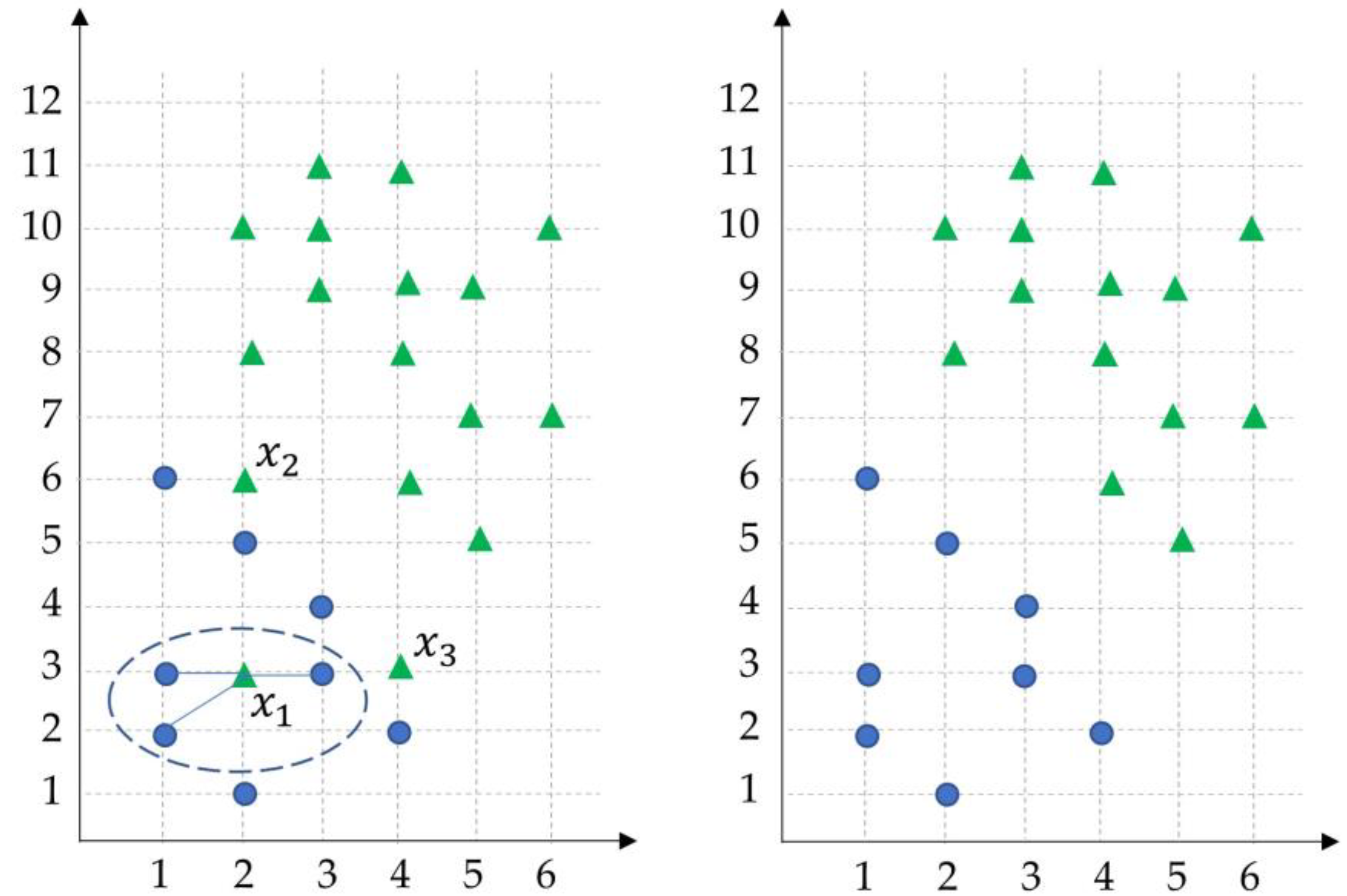
• Since LMT forest is an ensemble learning approach, it tends to achieve a better accuracy value than a single LMT model. Although some classifiers in the ensemble produce incorrect outputs, other classifiers may have the ability to correct these errors.
• As it is known, imbalanced datasets refer to classes with unequal observations. In other words, if the number of samples of a class is much higher than the others in a dataset. Imbalanced data make fault prediction models biased toward the majority of cases, resulting in the misclassification of the minority of cases. Our method provides a way to prevent class imbalance by using ENN; thus, it can successfully learn from cases belonging to all classes during the training stage.
• Another advantage of LMT forest is that it can be easily parallelized when it is needed. The algorithm is suitable for parallel and distributed environments.
• The other advantage of LMT forest is its implementation simplicity. It is mainly an ensemble-learning approach that contains several decision trees in a special manner.
• Inspired by the appealing structure of decision tree-based and logistic regression-based models, LMT forest is an interpretable and transparent approach, benefitting from explainable artificial intelligence (XAI). On the other hand, a deep learning (DL) model is difficult to interpret and explain because the composition of layers acts as a black box. In addition, variable selection is not easily possible since DL models solve feature engineering internally in a non-transparent way. Another drawback of DL is the high computational cost required to efficiently learn models since it has a large number of hyperparameters.
• One of the primary advantages of the presented method is that it is designed to apply to any type of data that is appropriate for the classification task. It does not require background or prior information about the given dataset. Therefore, it can be applied to different areas such as health, education, environment, and transportation.

3.3. Theoretical Expression

In this section, the theoretical expression of the proposed method is explained in detail. The LMT algorithm combines logistic regression and decision tree concepts to construct a tree. This kind of tree is highly acceptable since it deals with different data types (i.e., binary, nominal, numeric) and missing data, which are the LMT’s main benefits. This nonparametric method has the ability to predict class labels according to both qualitative and quantitative predictors. Moreover, it is possible to extract a sequence of rules from the tree regarding input values for the output predictions. In addition, LMT has been built on the basis of the LogitBoost classification algorithm for producing logistic models at each tree node and reducing probable outliers for improved performance. In LogitBoost classification, the tree is pruned by the classification and regression tree (CART) algorithm, which increases computational efficiency. One of the important advantages of LMT is the integration of logistic regression and classification by considering a validation technique to discover the number of LogitBoost iterations, and in this way, it prevents overfitting.

The algorithm uses a least-squares fit ($L_C\left(x\right)$), as given in the theoretical expression for each class $c$:

$$L_c\left(x\right)=\sum _{i=1}^n{\beta }_i{x}_i+{\beta }_0$$

(1)

where ${\beta }_i$ is the coefficient of the $i$-th element in vector $x$ for each ($i=\mathrm{1,2},3,\dots ,n$) and $n$ is the number of factors.

The algorithm also uses the logistic regression technique to calculate the posterior possibilities of tree nodes, expressed in Equation (2):

$$p\left(c|x\right)=\frac{\mathrm{e}\mathrm{x}\mathrm{p}\left(L_c\right(x\left)\right)}{\sum _{c^{\prime }=1}^r\mathrm{e}\mathrm{x}\mathrm{p}\left(L_{c^{\prime }}\right(x\left)\right)}$$

(2)

where r is the number of classes. This theoretical expression can be easily applicable for parameterizing the prediction process in the machine learning models.

The ENN technique is used to eliminate noisy data belonging to the majority class, as a common under-sampling approach. Different from an over-sampling algorithm, an under-sampling algorithm makes the classes balanced by removing some majority samples. ENN eliminates the samples of the majority class in accordance with the K-nearest neighbors (KNN) predictions. Given the dataset $D$, there is a subset of minority instances $N\subset D$ and a subset of majority instances $M\subset D$ such that $M\cup N=D$ and $\left|M\right|\gg \left|N\right|$. ENN aims to balance dataset $D$, such as $\left|M\right|\cong \left|N\right|$. If a sample $x_i\in M$ has more neighbors of a different class, this sample will be eliminated.

A theoretical expression for ignoring noise samples is provided by the ENN technique. Consider a majority sample $x_i\in M$, search to find k nearest neighbors of $x_i$, and then decide the class of $x_i$ according to its neighbors, which is denoted by $x_{ik}$. If the actual class $x_i$ differs from the predicted class of the KNN samples, then $x_i$ will be deleted ($x_{i\_delete}$) from the dataset $D$, otherwise, the algorithm keeps $x_i$. This theoretical expression is presented in Equation (3).

$$x_{i\_delete}=I\left(Class\right(x_i-x_{ik}\left)\right)$$

(3)

The parameter $k$ refers to the number of neighbors around $x_i$ belonging to the $M$ (majority) subset. This process will be repeated for every majority sample of $M$. In the case of multiclass problems, the subset $M$ can include instances from several majority classes.

Figure 2 illustrates an example of this technique. Assume that the number of neighbors is defined as three ($k=3$) and the Euclidean distance is used. Thus, the algorithm finds the three closest neighbors of each sample in the green-triangle class. For example, the sample $x_1$ is included in the majority class and its classification result (blue-circle) is in contrast to the original class (green-triangle); therefore, $x_1$ will be deleted. The same situation is also valid for the samples $x_2$ and $x_3$. The advantages of ENN are the removal of borderline samples to enhance the decision boundary and the facilitation of a classification algorithm to discriminate between minority and majority classes by eliminating noisy observations. Besides the mentioned advantages, ENN also improves computational efficiency by reducing the search space size.

The pseudo-code of the LMT forest method is given in Algorithm 1, regarding the input of the steel plate fault dataset and the output of fault types in steel plates as $D$ and $C$, respectively. Moreover, the input parameters of $e$ (ensemble size), $k$ (the number of neighbors), and $T$ (the testing set for classification) are supposed. In the first loop, based on the ENN technique, the algorithm investigates each instance in the given dataset $D$ separately. The k nearest neighbors are determined for each sample in the case of belonging to the majority class and added to the $O$ list. On the other hand, the samples of the minority class are directly added to this list without calculating their k-nearest neighbors. In the second loop, multiple training sets $D_i$ for ($i=1,2,3,\dots ,e$) are created by sampling the original dataset $D$ with replacement using the bootstrap method, where $e$ is the ensemble size. After that, the bagging technique is applied to build a set of models $H=\{H_1,H_2,\dots ,H_e\}$. In the last loop, each LMT model classifies a previously unseen query instance $x$ in the $T \mathrm{t}\mathrm{e}\mathrm{s}\mathrm{t} \mathrm{s}\mathrm{e}\mathrm{t}$. Afterward, the outputs of each model are aggregated using the majority voting technique to obtain the final fault type prediction. Eventually, the predicted fault class labels are gathered in the output list $C$.

Algorithm 1 Logistic Model Tree Forest.

Inputs:

$\hspace{1em}D:\mathrm{the} \mathrm{dataset} {D=\left\{d_i\right\}}_{i=1}^n$

e: ensemble size

k: the number of neighbors

T: testing set for classification

Output:

C: predicted fault types

Begin:

$\hspace{1em}\hspace{1em}O=Ø$

$\hspace{1em}\hspace{1em}\mathrm{for} i=1\mathrm{to} n \mathrm{do}$

$\hspace{1em}\hspace{1em}\hspace{1em}\hspace{1em}\mathrm{if} y ϵ M (\mathrm{majority} \mathrm{class})$

$\hspace{1em}\hspace{1em}\hspace{1em}\hspace{1em}\hspace{1em} \mathrm{if} \mathrm{KNN}\left({\mathrm{x}}_i\right)=y_i$

$\hspace{1em}\hspace{1em}\hspace{1em}\hspace{1em}\hspace{1em}\hspace{1em}\hspace{1em}\hspace{1em}\hspace{1em}\hspace{1em}O.\mathrm{Insert}(x_i, y_i)$

end if

else

$\hspace{1em}\hspace{1em}\hspace{1em}\hspace{1em}\hspace{1em}\hspace{1em}\hspace{1em}O.\mathrm{Insert}(x_i, y_i)$

end if

end for

for i = 1 to e do

Di = Bootstrap(O)

Hi = LMT(Di)

end for

$\hspace{1em} C=Ø$

foreach x in T

$\hspace{1em}\hspace{1em}\hspace{1em} c=\underset{y\in Y}{argmax}{\sum }_{i:y=H_i\left(x\right)}^{e}1$

$\hspace{1em}\hspace{1em}\hspace{1em} C=C \cup c$

end foreach

End Algorithm

Time complexity of the LMT forest algorithm is O(T + L(n)*m), in which T denotes the time needed for the ENN process, m is the ensemble size, and L(n) is the time required for running the LMT method on n objects.

3.4. Dataset Description

In the current study, a steel plate faults dataset [79] was applied to determine the efficiency of the proposed method. The dataset information is thoroughly listed in

Table 1. Dataset information.

Dataset Property	Attribute Property	Task	Instance	Feature	Missing Value	Field	Date	Web Hit
Multivariate	Integer, Real	Classification	1941	27	N/A	Physical	2010	111,062

. It is regarded as a multivariate dataset by the ability of classification tasks for training machine learning models aiming to automatic recognition of fault patterns. It covers attribute properties of integer and real values. Since 2010, this dataset has been widely utilized in the literature for contributing to the analysis of various methods over steel plate faults [20,21,22,23,24,25,26,27,28,29,30,31,32]. The dataset comprises 1941 records with different fault-type labels that can occur on steel surfaces.

The dataset contains 27 different features which are listed in

Table 2. The statistical properties of the dataset features.

No	Variable Name	Min	Mean	Max	Mode	Standard Deviation
1	X Maximum	4	617.9645	1713	212	497.6274
2	X Minimum	0	571.1360	1705	41	520.6907
3	Y Maximum	6724	1,650,738.7053	12,987,692	28,984	1,774,590
4	Y Minimum	6712	1,650,684.8681	12,987,661	1,803,992	1,774,578
5	Pixels Areas	2	1893.8784	152,655	52	5168.46
6	X Perimeter	2	111.8552	10,449	12	301.2092
7	Y Perimeter	1	82.9660	18,152	11	426.4829
8	Sum of Luminosity	250	206,312.1479	1,1591,414	7502	512,293.6
9	Maximum of Luminosity	37	130.1937	253	127	18.69099
10	Minimum of Luminosity	0	84.5487	203	101	32.13428
11	Length of Conveyer	1227	1459.1602	1794	1358	144.5778
12	Type of Steel (A300)	0	0.4003	1	0	0.490087
13	Type of Steel (A400)	0	0.5997	1	1	0.490087
14	Steel Plate Thickness	40	78.7378	300	40	55.08603
15	Empty Index	0	0.4142	0.9439	0.3333	0.137261
16	Edges Index	0	0.3317	0.9952	0.0604	0.299712
17	Square Index	0.0083	0.5708	1	1	0.271058
18	Outside X Index	0.0015	0.0334	0.8759	0.0059	0.058961
19	Edges X Index	0.0144	0.6105	1	1	0.243277
20	Edges Y Index	0.0484	0.8135	1	1	0.234274
21	Outside Global Index	0	0.5757	1	1	0.482352
22	Log of Areas	0.301	2.4924	5.1837	1.716	0.78893
23	Log X Index	0.301	1.3357	3.0741	0.9542	0.481612
24	Log Y Index	0	1.4033	4.2587	1.0792	0.454345
25	Luminosity Index	−0.9989	−0.1313	0.6421	−0.1851	0.148767
26	Orientation Index	−0.991	0.0833	0.9917	0	0.500868
27	Sigmoid of Areas	0.119	0.5854	1	1	0.339452

with their statistical properties, including minimum, mean, maximum, mode, and standard deviation of each one. The index features in the dataset are related to the quality of steel plates that include mechanical properties such as strength, toughness, elongation, shape, dimensional accuracy, appearance, and others.

The types of faults and the related number of instances are presented in

Table 3. Fault types and the number of instances in the dataset.

No	Fault Type	Number of Faults	Proportion of Faults (%)	Class Type
1	Pastry	158	8.14	Minority
2	Z-Scratch	190	9.79	Minority
3	K-Scratch	391	20.14	Moderate
4	Stains	72	3.71	Minority
5	Dirtiness	55	2.83	Minority
6	Bumps	402	20.71	Moderate
7	Other Faults	673	34.67	Majority
Total Number of Samples		1941

. As can be seen, the faults of steel plates are categorized into 7 types, including pastry, z-scratch, k-scratch, stains, dirtiness, bumps, and other faults. From the target class distribution in the dataset, it is observed that the class “Other Faults” (fault 7) represented the majority by 673 observations. Moreover, fault type 7 is not a distinct kind of fault; instead, it is a combined value of various faults that differs from faults 1 to 6. For this reason, specific treatment is required for fault 7. The instances in this class do not share special features; on the other hand, dominating predictors are not easy to obtain for training. In order to build a robust fault prediction model and minimize the number of false negatives, we applied the edited nearest neighbor technique to the dataset. This process can be approached by deleting samples whose class is different from the class of the majority of their k nearest neighbors. This data-preprocessing process is important since further classification is depending on this initial treatment.

4. Experiments

4.1. Experimental Design

The main aim of this research was to correctly classify the surface defects in stainless steel plates by seven types of faults through developing a machine learning-based model for fault prediction. For this purpose, the LMT forest method was proposed and its effectiveness was proved on a fault prediction dataset [79]. We developed our method by C# language using the Weka library [80]. In the experiments, we used the 10-fold cross-validation technique to train and test the classifiers. In this low-bias technique, the dataset is randomly split into 10 folds or parts, and then 1 fold is reserved as a test set, and the other 9 folds are considered as the training set. The validation process was repeated 10 times and the average classification rate was calculated. In addition, various types of evaluation measures were utilized to experimentally prove the theoretical expression of the proposed LMT forest model, including accuracy (ACC), recall (R), precision (PR), and F-measure (FM), which are formulated in Equations (4) to (7), respectively.

$$ACC=\frac{TP+TN}{TP+TN+FP+FN}$$

(4)

$$R=\frac{TP}{TP+FN}$$

(5)

$$PR=\frac{TP}{TP+FP}$$

(6)

$$FM=\frac{2TP}{2TP+FP+FN}$$

(7)

where

• True positive (TP) defines the number of positive classes, which are predicted correctly by the classifier.
• True negative (TN) defines the number of negative classes, which are predicted correctly by the classifier.
• False positive (FP) defines the number of positive classes, which are predicted incorrectly by the classifier.
• False negative (FN) defines the number of negative classes, which are predicted incorrectly by the classifier.

4.2. Experimental Results

The balanced dataset was divided as a training set and test set through the 10-fold cross-validation technique with the aim of applying the proposed LMT forest method to it. According to this approach, the results of each fold are separately given in

Table 4. The comparison of random forest and the proposed LMT forest in terms of accuracy.

Fold Number	Accuracy (%)
	Random Forest [81]	LMT Forest (Proposed)
1	77.9487	85.4545
2	79.8969	85.3659
3	78.8660	88.4146
4	81.9588	88.4146
5	82.4742	85.9756
6	80.4124	90.2439
7	80.4124	87.1951
8	77.3196	84.7561
9	78.8660	85.9756
10	77.3196	84.7561
Average	79.547	86.655

. As can be seen, our proposed model outperformed the well-known random forest method [81] in terms of classification accuracy. On average, LMT forest (86.655%) achieved higher accuracy than random forest (79.547%) with an improvement of over 7%. Therefore, our model can be effectively used in steel production lines.

The main reason behind this improvement is that our method takes into consideration the distribution of class instances and makes the dataset balanced. The steel plate faults dataset was regarded as an imbalanced dataset since the proportion of a class is highly skewed to the total number of instances. The ratio of the majority class was 35%, while the proportions of the other six minority classes were low. Furthermore, the class “Other Faults” could contain noisy samples since it did not have a single special kind of fault; instead, it is a combination of several faults that differ from other faults. To overcome this problem, we applied the ENN method to the dataset by setting the parameter k to 3 and obtained balanced and noise-free data. As a result, the number of instances decreased from 1941 to 1641 after the balancing approach.

The comparison of LMT forest and random forest models is given in Figure 3 in terms of several evaluation metrics such as precision, recall, F-measure, Matthews correlation coefficient (MCC), receiver operating characteristic (ROC) area, and precision–recall (PRC) area. Our method improved performance according to the all mentioned metrics, compared to the existing method [81]. The key reason for low precision and recall of classification is the use of an unbalanced and noisy training dataset. Our method solves these problems by applying the ENN technique.

The most significant input parameter of the LMT forest method is the number of trees. Parameter tuning was performed by implementing it with from 1 to 100 trees with increments of 10 to gain the highest accuracy of the method. The results are presented in

Table 5. The accuracy rates obtained by LMT forest for different numbers of trees.

Number of Trees	Accuracy (%)
1	74.858
10	84.887
20	86.106
30	86.106
40	86.472
50	86.472
60	86.655
70	86.533
80	86.594
90	86.289
100	86.228

. It should be addressed that these outputs are calculated by averaging the results of the 10 folds. The evaluations revealed that the LMT forest with 60 trees had the highest accuracy of 86.655% in comparison with the other number of trees. While there was an increase up to the peak (60 trees), from that point on, the accuracy dropped slightly. The main reason behind this pattern can be explained by considering the tradeoff between generalization ability and overfitting. When a small number of trees are included, the likelihood of misclassification increases due to instability like with a single decision tree. Once the ensemble size is small, each classifier will have a big effect on the final prediction. In addition, if the qualities of ensemble members are poor, the overall performance is influenced accordingly. Therefore, it is required to increase the number of trees in the ensemble to reduce the influence of members that are of low quality. On the other hand, when a large number of trees are available, the algorithm is at risk of overfitting. Increasing the ensemble size may not significantly increase performance even it brings higher computational costs. Therefore, a large number of classifiers cannot guarantee a remarkably more satisfying result.

The confusion matrix obtained by the LMT forest method is presented in

Table 6. The confusion matrix that was obtained by LMT forest.

	A	B	C	D	E	F	G
A	107	0	0	0	2	30	19
B	0	176	2	0	0	7	5
C	0	0	376	2	0	5	8
D	0	0	0	66	0	3	3
E	2	0	0	0	49	3	1
F	20	4	3	3	6	334	32
G	13	2	6	1	1	36	314

for all fault classes separately. In this matrix, steel fault classes including pastry, z-scratch, k-scratch, stains, dirtiness, bumps, and other faults are represented by A to G, respectively. The matrix summarizes the correct and incorrect predictions of the LMT forest model with the count values. The robustness of the model for predicting steel plate faults was firmly confirmed with the high diagonal elements of the matrix (107, 176, 376, 66, 49, 334, and 314) for each class and with low off-diagonal elements. It is clear that the constructed model generally had no trouble in classifying all fault types. For example, 376 out of 391 k-scratch faults were predicted accurately; however, only 15 of them were misclassified by the model. Even though each fault type was distinguished with high accuracy, the algorithm slightly confused the pastry fault with other fault types. This is probably because of the fact that the behavior of this fault is a little bit similar to the other fault types, especially bump faults.

The importance scores of features for the balanced steel plate faults dataset are given in

Table 7. Importance of features obtained by the Pearson correlation method.

Feature	Score	Feature	Score	Feature	Score
Log X Index	0.3064	Log Y Index	0.2359	Orientation Index	0.1678
Log of Areas	0.3020	Minimum of Luminosity	0.2246	Empty Index	0.1569
Type of Steel (A300)	0.2819	X Maximum	0.2190	Outside Global Index	0.1368
Type of Steel (A400)	0.2819	Length of Conveyer	0.2144	Edges X Index	0.1326
Edges Y Index	0.2772	Sigmoid of Areas	0.2140	Maximum of Luminosity	0.1138
Sum of Luminosity	0.2699	Edges Index	0.2009	Luminosity Index	0.1065
Outside X Index	0.2655	X Perimeter	0.1938	Y Perimeter	0.0868
X Minimum	0.2475	Steel Plate Thickness	0.1823	Y Maximum	0.0857
Pixels Areas	0.2430	Square Index	0.1762	Y Minimum	0.0857

. Importance scores of features contribute to having a better understanding of the effect of features on the prediction results. Here, we applied the Pearson correlation method over the steel plate faults to investigate the most significant features in the occurrence of steel plate faults. The Pearson correlation method is one of the common covariance-based approaches to utilize for numeric values with the objective of determining the linear relationship between those variables, and thus revealing their importance compared to each other through measuring the linear correlation. The Pearson correlation score is a number in the range from −1 to +1, demonstrating the direction and strength of features in a dataset, in which 0 means no correlation, and where −1 and +1 show the totally negative and positive correlations, respectively. In addition, the direction from 0 to −1 increases negativity, and vice versa, the direction from 0 to +1 increases positivity. Interpretation of the Pearson correlation method is uncomplicated and its produced data have better statistical properties, along with the magnitude of the correlation, association, and direction of relations [82,83,84,85,86]. According to the results given in Table 7, the predictor importance of the “Log X Index” and “Log of Areas” with the values of 0.3046 and 0.3020 are the highest ones. In addition, the prediction importance of the “Y Minimum” and “Y Maximum” with the value of 0.0857 is the lowest one.

The structure of the logistic model tree with 41 nodes and 21 leaves is illustrated in Figure 4. It is possible to extract rules from this tree by tracing each branch from root to leaf. For example, at the second level of the tree, if the value of the “Pixels Areas” feature is greater than 26, then the sub-tree of the “Type of Steel (A300)” node will be followed, or else a decision is made since the leaf node is reached. Compared with features in the tree branches, the feature in the root of the tree has a stronger effect on predicting the output. Therefore, the tree indicates that the “Log of Areas” feature has a high impact on decision making.

4.3. Comparison with the State-of-the-Art Methods

In this section, the proposed LMT forest method is compared with the state-of-the-art methods [20,21,22,23,24,25,26,27,28,29,30,31,32]. The results of previous studies on the same dataset are given in

Table 8. The comparison of LMT forest with the state-of-the-art methods on the same dataset.

Reference	Year	Method	Accuracy (%)
Shu et al. [20]	2023	Support vector machines with extended decision label annotation (ELA)	77.53
		C4.5 with extended decision label annotation (ELA)	75.42
Agrawal and Adane [21]	2022	Long short-term memory (LSTM)	75.62
		Random forest (RF)	76.11
		Principal component analysis-based decision tree forest (PDTF)	75.19
		Improved PDTF (I-PDTF)	76.09
Ju et al. [22]	2022	Radial base function-based support vector machine (RBF-SVM)	62.80
		Classification and regression trees (CARTs)	62.99
		Neighborhood classifier (NEC)	65.68
Zhang et al. [23]	2022	Bi-selection method based on fuzzy rough sets (BSFRSs)	69.18
		Central density-based instance selection MQRWA (CDIS-MQRWA)	71.14
		Edited nearest neighbor MQRWA (ENN-MQRWA)	73.72
Mohamed and Samsudin [24]	2021	Naive Bayes	69.20
		K-nearest neighbors (KNNs)	71.80
		Decision tree (DT)	75.10
Nkonyana et al. [25]	2019	Random forest	77.80
		Support vector machines (SVMs)	73.60
		Artificial neural network (ANN)	69.60
Srivastava [26]	2019	Decision tree	76.04
		Random forest	79.39
		AdaBoost	78.41
		K-nearest neighbors	71.35
		Support vector machines	74.90
Mohamed et al. [27]	2019	Naive Bayes + information gain (IGO)	66.70
		K-nearest neighbor (KNN) + hybrid bat algorithm (BkMDFS)	72.40
Mary [28]	2018	Back-propagation neural network	75.27
Zhang et al. [29]	2018	Neural network (NN)	77.28
		Classification and regression trees (CARTs)	79.08
		Linear support vector machine	72.08
		Minimal-redundancy-maximal-relevance (mRMR)-Wrapper + CART	79.34
Thirukovalluru et al. [30]	2016	Support vector machine	75.27
		Random forest	78.11
Halawani [31]	2014	AdaBoost.M1	81.92
		Random forest	79.96
Buscema et al. [32]	2010	Meta-consensus	77.00
		ArcX4	80.35
		AdaBoost.M1	79.31
		Quadratic Bayesian classifier (QDC)	77.20
		Naive Bayesian combiner (BayesComb)	71.95
		Bayesian linear classifier (LDC)	74.25
		Sine network (SN)	74.16
		Dempster–Shafer combination	80.58
		Direct KNN decision dependent (DynDdDirectKnn)	77.40
Proposed Method		Logistic model tree forest	86.655

. These results were directly taken from the articles investigated by authors on the same dataset [79] as our work for the prediction of steel plate faults. In the table, various machine learning methods (e.g., KNN, SVM, ANN, etc.) are included to compare them with our method. For instance, LMT forest (86.655%) outperformed KNN (71.80%) [24], SVM (73.60%) [25], NN (77.28%) [29], and naive Bayes (66.70%) [27] methods. The reason behind this improvement is probably because of the fact that these standard methods build a single classifier, while our method constructs multiple classifiers in an ensemble manner. In addition, LMT forest performed better than other tree-based machine-learning approaches in terms of accuracy metrics. For example, LMT forest (86.655%) validated its outperformance over RF (77.80%) [25], DT (76.04%) [26], and CART (79.08%) [29] on the same steel plate faults dataset. A possible reason behind this is that LMT builds a different type of tree, which is a classification tree with logistic regression functions at the leaves.

The LMT forest model achieved higher accuracy compared to many other techniques, e.g., BSFRS (69.18%) [23], IGO (66.70%) [27], and SN (74.16%) [32]. The accuracy of the proposed model is also the highest in comparison with deep learning models such as LSTM (75.62%) [21]. In brief, all these evaluations indicate the outperformance of LMT forest. Therefore, our presented model can be efficiently utilized for the fault prediction of steel plates.

The main reason behind the superiority of our method over the aforementioned methods is that it takes into consideration the distribution of class instances and makes the dataset balanced. Note that in a standard machine learning model, imbalanced data ignore beneficial information about the dataset itself that is essential for the construction of classifiers. Additionally, in an ensemble method, the sampled instances from an imbalanced dataset are most likely biased instances that lead to an inaccurate representation of the dataset. The steel plate faults dataset was regarded as an imbalanced dataset since the proportion of a class is highly skewed to the total number of instances. The ratio of the majority class was 35%, while the proportions of the other six minority classes were low. Furthermore, the class “Other Faults” could contain noisy samples since it did not have a single special kind of fault; instead, it is a combination of several faults that differ from other faults. To overcome this problem, we applied the ENN technique to the dataset and obtained class-balanced and noise-free data. As a result, the performance was improved in terms of accuracy.

The results show the superiority of LMT forest with an accuracy of 86.655% over the best existing method, namely AdaBoost.M1 [31], with an accuracy of 81.92%. Therefore, the proposed method performed better with approximately 5% improvement compared to the best method in Table 8. The best improvement (23.86%) achieved over the RBF-SVM method [22]. Accordingly, the LMT forest model can be successfully utilized in steel product manufacturing with the objective of fault prediction and thus making the necessary arrangements to handle faults with regard to the high accuracy of our presented model.

5. Conclusions and Future Works

In this study, we proposed a novel machine learning method, entitled logistic model tree forest (LMT forest), for predicting and identifying different types of steel plate faults. In addition to the importance of faultless steel plate production, the automation of fault prediction considerably contributes to reducing production costs and minimizing the necessary time for monitoring. The results revealed that the developed model is appropriately capable of being used during industrial production, and outstandingly contributes to decision making for faults handling in the steel plate manufacturing process. Our method is applicable to the steel plate manufacturing to improve the efficiency of industrial steel products.

The key outcomes of our study are listed as follows:

• LMT forest integrates decision tree and logistic regression approaches to profit from the benefits of both techniques.
• In this study, it was revealed that the ensemble of classifiers instead of a single classifier could attain better performance.
• Different ensemble sizes of 1 to 100 with 10 intervals were tested, and finally, we decided on 60 trees, since after that the accuracy began to decrease slightly.
• The confusion matrix showed that each fault type was distinguished with high accuracy; however, the pastry fault was slightly confused with other fault types by the algorithm.
• According to the results of the Pearson correlation method, the “Log X Index” and “Log of Areas” variables are the most essential features in the decision-making process.
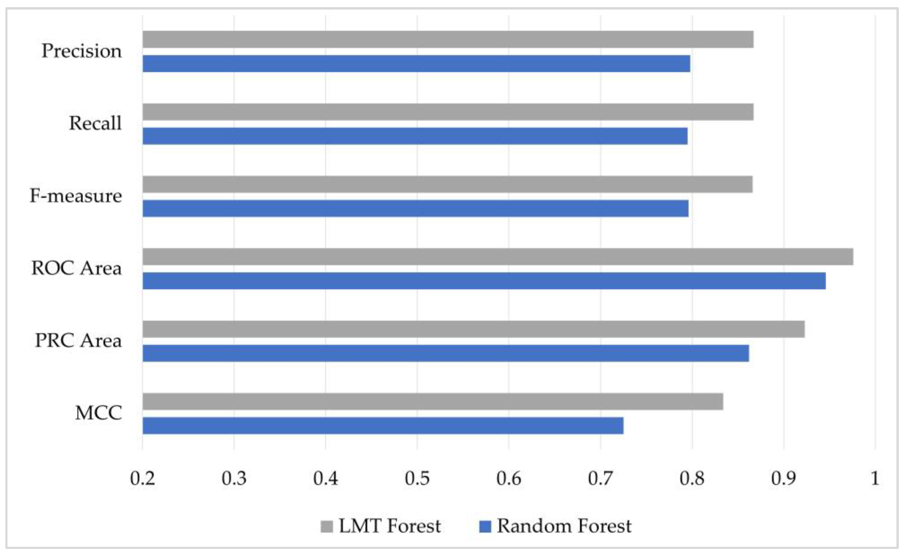
• The superiority of the proposed LMT forest method (86.65%) over the well-known random forest method (79.547%) was approved on the same dataset.
• The proposed model (86.65%) achieved higher performance when compared to the state-of-the-art methods [20,21,22,23,24,25,26,27,28,29,30,31,32] in terms of accuracy. Improvements ranging from 5 to 24% were demonstrated compared to the aforementioned methods.

As a future work, the LMT forest method can be utilized for predictive maintenance in IoT-based manufacturing. Our method can be efficiently applied to other datasets for different purposes. In addition, it is possible to collect greater amounts of data from steel production factories, which can include different fault classes.

References

1. Landwehr, N.; Hall, M.; Frank, E. Logistic Model Trees. Mach. Learn. 2005, 59, 161–205. [Google Scholar] [CrossRef] [Green Version]
2. Kamali Maskooni, E.; Naghibi, S.A.; Hashemi, H.; Berndtsson, R. Application of Advanced Machine Learning Algorithms to Assess Groundwater Potential Using Remote Sensing-Derived Data. Remote Sens. 2020, 12, 2742. [Google Scholar] [CrossRef]
3. Debnath, P.; Chittora, P.; Chakrabarti, T.; Chakrabarti, P.; Leonowicz, Z.; Jasinski, M.; Gono, R.; Jasińska, E. Analysis of Earthquake Forecasting in India Using Supervised Machine Learning Classifiers. Sustainability 2021, 13, 971. [Google Scholar] [CrossRef]
4. Zhao, X.; Chen, W. Optimization of Computational Intelligence Models for Landslide Susceptibility Evaluation. Remote Sens. 2020, 12, 2180. [Google Scholar] [CrossRef]
5. Davis, J.D.; Wang, S.; Festa, E.K.; Luo, G.; Moharrer, M.; Bernier, J.; Ott, B.R. Detection of Risky Driving Behaviors in the Naturalistic Environment in Healthy Older Adults and Mild Alzheimer’s Disease. Geriatrics 2018, 3, 13. [Google Scholar] [CrossRef] [Green Version]
6. Lee, S.-W.; Kung, H.-C.; Huang, J.-F.; Hsu, C.-P.; Wang, C.-C.; Wu, Y.-T.; Wen, M.-S.; Cheng, C.-T.; Liao, C.-H. The Clinical Application of Machine Learning-Based Models for Early Prediction of Hemorrhage in Trauma Intensive Care Units. J. Pers. Med. 2022, 12, 1901. [Google Scholar] [CrossRef] [PubMed]
7. Reyes-Bueno, F.; Loján-Córdova, J. Assessment of Three Machine Learning Techniques with Open-Access Geographic Data for Forest Fire Susceptibility Monitoring—Evidence from Southern Ecuador. Forests 2022, 13, 474. [Google Scholar] [CrossRef]
8. Han, J.; Nur, A.S.; Syifa, M.; Ha, M.; Lee, C.-W.; Lee, K.-Y. Improvement of Earthquake Risk Awareness and Seismic Literacy of Korean Citizens through Earthquake Vulnerability Map from the 2017 Pohang Earthquake, South Korea. Remote Sens. 2021, 13, 1365. [Google Scholar] [CrossRef]
9. Nhu, V.-H.; Mohammadi, A.; Shahabi, H.; Ahmad, B.B.; Al-Ansari, N.; Shirzadi, A.; Geertsema, M.R.; Kress, V.; Karimzadeh, S.; Valizadeh Kamran, K.; et al. Landslide Detection and Susceptibility Modeling on Cameron Highlands (Malaysia): A Comparison between Random Forest, Logistic Regression and Logistic Model Tree Algorithms. Forests 2020, 11, 830. [Google Scholar] [CrossRef]
10. Nhu, V.-H.; Shirzadi, A.; Shahabi, H.; Singh, S.K.; Al-Ansari, N.; Clague, J.J.; Jaafari, A.; Chen, W.; Miraki, S.; Dou, J.; et al. Shallow Landslide Susceptibility Mapping: A Comparison between Logistic Model Tree, Logistic Regression, Naïve Bayes Tree, Artificial Neural Network, and Support Vector Machine Algorithms. Int. J. Environ. Res. Public Health 2020, 17, 2749. [Google Scholar] [CrossRef] [Green Version]
11. Pham, B.T.; Phong, T.V.; Nguyen, H.D.; Qi, C.; Al-Ansari, N.; Amini, A.; Ho, L.S.; Tuyen, T.T.; Yen, H.P.H.; Ly, H.-B.; et al. A Comparative Study of Kernel Logistic Regression, Radial Basis Function Classifier, Multinomial Naïve Bayes, and Logistic Model Tree for Flash Flood Susceptibility Mapping. Water 2020, 12, 239. [Google Scholar] [CrossRef] [Green Version]
12. Charton, E.; Meurs, M.-J.; Jean-Louis, L.; Gagnon, M. Using Collaborative Tagging for Text Classification: From Text Classification to Opinion Mining. Informatics 2014, 1, 32–51. [Google Scholar] [CrossRef] [Green Version]
13. Amirruddin, A.D.; Muharam, F.M.; Ismail, M.H.; Tan, N.P.; Ismail, M.F. Synthetic Minority Over-Sampling TEchnique (SMOTE) and Logistic Model Tree (LMT)-Adaptive Boosting Algorithms for Classifying Imbalanced Datasets of Nutrient and Chlorophyll Sufficiency Levels of Oil Palm (Elaeis Guineensis) Using Spectroradiometers and Unmanned Aerial Vehicles. Comput. Electron. Agric. 2022, 193, 106646. [Google Scholar] [CrossRef]
14. Wang, L.; You, Z.-H.; Chen, X.; Li, Y.-M.; Dong, Y.-N.; Li, L.-P.; Zheng, K. LMTRDA: Using Logistic Model Tree to Predict MiRNA-Disease Associations by Fusing Multi-Source Information of Sequences and Similarities. PLoS Comput. Biol. 2019, 15, e1006865. [Google Scholar] [CrossRef] [Green Version]
15. Kabir, E.; Siuly; Zhang, Y. Epileptic Seizure Detection from EEG Signals Using Logistic Model Trees. Brain Inf. 2016, 3, 93–100. [Google Scholar] [CrossRef] [PubMed] [Green Version]
16. Cheng, C.-H.; Yang, J.-H.; Liu, P.-C. Rule-Based Classifier Based on Accident Frequency and Three-Stage Dimensionality Reduction for Exploring the Factors of Road Accident Injuries. PLoS ONE 2022, 17, e0272956. [Google Scholar] [CrossRef] [PubMed]
17. Jha, S.K.; Ahmad, Z. An Effective Feature Generation and Selection Approach for Lymph Disease Recognition. Comp. Model. Eng. Sci. 2021, 129, 567–594. [Google Scholar] [CrossRef]
18. Ayyappan, G.; Babu, R.V. Knowledge Construction on NIV of COVID-19 for Managing the Patients by ML Techniques. Indian J. Comput. Sci. Eng. 2023, 14, 117–129. [Google Scholar] [CrossRef]
19. Gorka, M.; Thomas, A.; Bécue, A. Differentiating Individuals through the Chemical Composition of Their Fingermarks. Forensic Sci. Int. 2023, 346, 111645. [Google Scholar] [CrossRef]
20. Shu, W.; Yan, Z.; Yu, J.; Qian, W. Information Gain-Based Semi-Supervised Feature Selection for Hybrid Data. Appl. Intell. 2022, 53, 7310–7325. [Google Scholar] [CrossRef]
21. Agrawal, L.; Adane, D. Ensembled Approach to Heterogeneous Data Streams. Int. J. Next Gener. Comput. 2022, 13, 1014–1020. [Google Scholar] [CrossRef]
22. Ju, H.; Ding, W.; Shi, Z.; Huang, J.; Yang, J.; Yang, X. Attribute Reduction with Personalized Information Granularity of Nearest Mutual Neighbors. Inf. Sci. 2022, 613, 114–138. [Google Scholar] [CrossRef]
23. Zhang, X.; Mei, C.; Li, J.; Yang, Y.; Qian, T. Instance and Feature Selection Using Fuzzy Rough Sets: A Bi-Selection Approach for Data Reduction. IEEE Trans. Fuzzy Syst. 2022, 31, 1–15. [Google Scholar] [CrossRef]
24. Mohamed, R.; Samsudin, N.A. An Optimized Discretization Approach Using K-Means Bat Algorithm. Turk. J. Comput. Math. Educ. 2021, 12, 1842–1851. [Google Scholar] [CrossRef]
25. Nkonyana, T.; Sun, Y.; Twala, B.; Dogo, E. Performance Evaluation of Data Mining Techniques in Steel Manufacturing Industry. Procedia Manuf. 2019, 35, 623–628. [Google Scholar] [CrossRef]
26. Srivastava, A.K. Comparison analysis of machine learning algorithms for steel plate fault detection. Int. Res. J. Eng. Technol. 2019, 6, 1231–1234. [Google Scholar]
27. Mohamed, R.; Yusof, M.M.; Wahid, N.; Murli, N.; Othman, M. Bat Algorithm and K-Means Techniques for Classification Performance Improvement. Indones. J. Electr. Eng. Comput. Sci. 2019, 15, 1411. [Google Scholar] [CrossRef]
28. Mary, D. Constructing optimized Neural Networks using Genetic Algorithms and Distinctiveness. In Proceedings of the 1st ANU Bio-inspired Computing Conference (ABCs 2018), Canberra, Australia, 20 July 2018; pp. 1–8. [Google Scholar]
29. Zhang, X.; Mei, C.; Chen, D.; Yang, Y. A Fuzzy Rough Set-Based Feature Selection Method Using Representative Instances. Knowl.-Based Syst. 2018, 151, 216–229. [Google Scholar] [CrossRef]
30. Thirukovalluru, R.; Dixit, S.; Sevakula, R.K.; Verma, N.K.; Salour, A. Generating Feature Sets for Fault Diagnosis Using Denoising Stacked Auto-Encoder. In Proceedings of the IEEE International Conference on Prognostics and Health Management (ICPHM), Ottawa, ON, Canada, 20–22 June 2016; pp. 1–7. [Google Scholar] [CrossRef]
31. Halawani, S.M. A study of decision tree ensembles and feature selection for steel plates faults detection. Int. J. Tech. Res. Appl. 2014, 2, 127–131. [Google Scholar]
32. Buscema, M.; Tastle, W.J. A New Meta-Classifier. In Proceedings of the Annual Meeting of the North American Fuzzy Information Processing Society, Toronto, ON, Canada, 12–14 July 2010; pp. 1–7. [Google Scholar] [CrossRef]
33. Ma, L.; Jiang, H.; Ma, T.; Zhang, X.; Shen, Y.; Xia, L. Fault Prediction of Rolling Element Bearings Using the Optimized MCKD–LSTM Model. Machines 2022, 10, 342. [Google Scholar] [CrossRef]
34. Xu, Q.; Jiang, H.; Zhang, X.; Li, J.; Chen, L. Multiscale Convolutional Neural Network Based on Channel Space Attention for Gearbox Compound Fault Diagnosis. Sensors 2023, 23, 3827. [Google Scholar] [CrossRef]
35. Pollak, A.; Temich, S.; Ptasiński, W.; Kucharczyk, J.; Gąsiorek, D. Prediction of Belt Drive Faults in Case of Predictive Maintenance in Industry 4.0 Platform. Appl. Sci. 2021, 11, 10307. [Google Scholar] [CrossRef]
36. Glowacz, A. Thermographic Fault Diagnosis of Shaft of BLDC Motor. Sensors 2022, 22, 8537. [Google Scholar] [CrossRef] [PubMed]
37. Javed, M.R.; Shabbir, Z.; Asghar, F.; Amjad, W.; Mahmood, F.; Khan, M.O.; Virk, U.S.; Waleed, A.; Haider, Z.M. An Efficient Fault Detection Method for Induction Motors Using Thermal Imaging and Machine Vision. Sustainability 2022, 14, 9060. [Google Scholar] [CrossRef]
38. Chen, Y.; Ding, Y.; Zhao, F.; Zhang, E.; Wu, Z.; Shao, L. Surface Defect Detection Methods for Industrial Products: A Review. Appl. Sci. 2021, 11, 7657. [Google Scholar] [CrossRef]
39. Çınar, Z.M.; Abdussalam Nuhu, A.; Zeeshan, Q.; Korhan, O.; Asmael, M.; Safaei, B. Machine Learning in Predictive Maintenance towards Sustainable Smart Manufacturing in Industry 4.0. Sustainability 2020, 12, 8211. [Google Scholar] [CrossRef]
40. Shim, J.; Kang, S.; Cho, S. Active Inspection for Cost-Effective Fault Prediction in Manufacturing Process. J. Process Control 2021, 105, 250–258. [Google Scholar] [CrossRef]
41. Fernandes, M.; Corchado, J.M.; Marreiros, G. Machine Learning Techniques Applied to Mechanical Fault Diagnosis and Fault Prognosis in the Context of Real Industrial Manufacturing Use-Cases: A Systematic Literature Review. Appl. Intell. 2022, 52, 14246–14280. [Google Scholar] [CrossRef] [PubMed]
42. Uppal, M.; Gupta, D.; Juneja, S.; Dhiman, G.; Kautish, S. Cloud-Based Fault Prediction Using IoT in Office Automation for Improvisation of Health of Employees. J. Healthcare Eng. 2021, 2021, 8106467. [Google Scholar] [CrossRef]
43. Kosuru, V.S.R.; Kavasseri Venkitaraman, A. A Smart Battery Management System for Electric Vehicles Using Deep Learning-Based Sensor Fault Detection. World Electr. Veh. J. 2023, 14, 101. [Google Scholar] [CrossRef]
44. Gong, L.; Liu, B.; Fu, X.; Jabbari, H.; Gao, S.; Yue, W.; Yuan, H.; Fu, R.; Wang, Z. Quantitative Prediction of Sub-Seismic Faults and Their Impact on Waterflood Performance: Bozhong 34 Oilfield Case Study. J. Pet. Sci. Eng. 2019, 172, 60–69. [Google Scholar] [CrossRef]
45. Dashti, R.; Daisy, M.; Mirshekali, H.; Shaker, H.R.; Hosseini Aliabadi, M. A Survey of Fault Prediction and Location Methods in Electrical Energy Distribution Networks. Measurement 2021, 184, 109947. [Google Scholar] [CrossRef]
46. Carrera, Á.; Alonso, E.; Iglesias, C.A. A Bayesian Argumentation Framework for Distributed Fault Diagnosis in Telecommunication Networks. Sensors 2019, 19, 3408. [Google Scholar] [CrossRef] [PubMed] [Green Version]
47. Bai, Y.; Zhao, J. A Novel Transformer-Based Multi-Variable Multi-Step Prediction Method for Chemical Process Fault Prognosis. Process Saf. Environ. Prot. 2023, 169, 937–947. [Google Scholar] [CrossRef]
48. Zhang, P.; Cui, Z.; Wang, Y.; Ding, S. Application of BPNN Optimized by Chaotic Adaptive Gravity Search and Particle Swarm Optimization Algorithms for Fault Diagnosis of Electrical Machine Drive System. Electr. Eng. 2021, 104, 819–831. [Google Scholar] [CrossRef]
49. Abro, J.H.; Li, C.; Shafiq, M.; Vishnukumar, A.; Mewada, S.; Malpani, K.; Osei-Owusu, J. Artificial Intelligence Enabled Effective Fault Prediction Techniques in Cloud Computing Environment for Improving Resource Optimization. Sci. Program. 2022, 2022, 1–7. [Google Scholar] [CrossRef]
50. Doorwar, A.; Bhalja, B.R.; Malik, O.P. Novel Approach for Synchronous Generator Protection Using New Differential Component. IEEE Trans. Energy Convers. 2022, 38, 180–191. [Google Scholar] [CrossRef]
51. Tsioumpri, E.; Stephen, B.; McArthur, S.D.J. Weather Related Fault Prediction in Minimally Monitored Distribution Networks. Energies 2021, 14, 2053. [Google Scholar] [CrossRef]
52. Shahbazi, Z.; Byun, Y.-C. Smart Manufacturing Real-Time Analysis Based on Blockchain and Machine Learning Approaches. Appl. Sci. 2021, 11, 3535. [Google Scholar] [CrossRef]
53. Samanta, A.; Chowdhuri, S.; Williamson, S.S. Machine Learning-Based Data-Driven Fault Detection/Diagnosis of Lithium-Ion Battery: A Critical Review. Electronics 2021, 10, 1309. [Google Scholar] [CrossRef]
54. Lin, S.-L. Application of Machine Learning to a Medium Gaussian Support Vector Machine in the Diagnosis of Motor Bearing Faults. Electronics 2021, 10, 2266. [Google Scholar] [CrossRef]
55. Jiang, F.; Norlund, P. Seismic attribute-guided automatic fault prediction by deep learning. In Proceedings of the EAGE 2020 Annual Conference Exhibition, Online, 8–11 December 2020; European Association of Geoscientists & Engineers: Utrecht, The Netherlands, 2020; Volume 2020, pp. 1–5. [Google Scholar] [CrossRef]
56. Wang, S.; Si, X.; Cai, Z.; Cui, Y. Structural Augmentation in Seismic Data for Fault Prediction. Appl. Sci. 2022, 12, 9796. [Google Scholar] [CrossRef]
57. Li, Y. A Fault Prediction and Cause Identification Approach in Complex Industrial Processes Based on Deep Learning. Comput. Intell. Neurosci. 2021, 2021, 6612342. [Google Scholar] [CrossRef]
58. Yang, H.-S.; Kim, Y.-S. Design and Implementation of Machine Learning-Based Fault Prediction System in Cloud Infrastructure. Electronics 2022, 11, 3765. [Google Scholar] [CrossRef]
59. Zhao, Y.; Li, D.; Dong, A.; Kang, D.; Lv, Q.; Shang, L. Fault Prediction and Diagnosis of Wind Turbine Generators Using SCADA Data. Energies 2017, 10, 1210. [Google Scholar] [CrossRef] [Green Version]
60. Yuan, T.; Sun, Z.; Ma, S. Gearbox Fault Prediction of Wind Turbines Based on a Stacking Model and Change-Point Detection. Energies 2019, 12, 4224. [Google Scholar] [CrossRef] [Green Version]
61. Wan, L.; Li, H.; Chen, Y.; Li, C. Rolling Bearing Fault Prediction Method Based on QPSO-BP Neural Network and Dempster–Shafer Evidence Theory. Energies 2020, 13, 1094. [Google Scholar] [CrossRef]
62. Yang, J.; Li, J.-D. Fault Prediction Algorithm for Offshore Wind Energy Conversion System Based on Machine Learning. In Proceedings of the International Conference on High Performance Big Data and Intelligent Systems (HPBD&IS), Macau, China, 5–7 December 2021; pp. 291–296. [Google Scholar] [CrossRef]
63. Fernandes, S.; Antunes, M.; Santiago, A.R.; Barraca, J.P.; Gomes, D.; Aguiar, R.L. Forecasting Appliances Failures: A Machine-Learning Approach to Predictive Maintenance. Information 2020, 11, 208. [Google Scholar] [CrossRef] [Green Version]
64. Tsai, M.-F.; Chu, Y.-C.; Li, M.-H.; Chen, L.-W. Smart Machinery Monitoring System with Reduced Information Transmission and Fault Prediction Methods Using Industrial Internet of Things. Mathematics 2020, 9, 3. [Google Scholar] [CrossRef]
65. Syafrudin, M.; Alfian, G.; Fitriyani, N.; Rhee, J. Performance Analysis of IoT-Based Sensor, Big Data Processing, and Machine Learning Model for Real-Time Monitoring System in Automotive Manufacturing. Sensors 2018, 18, 2946. [Google Scholar] [CrossRef] [Green Version]
66. Yuan, H.; Zhang, Z.; Yuan, P.; Wang, S.; Wang, L.; Yuan, Y. A Microgrid Alarm Processing Method Based on Equipment Fault Prediction and Improved Support Vector Machine Learning. J. Phys. Conf. Ser. 2020, 1639, 012041. [Google Scholar] [CrossRef]
67. Zhang, X.; Wang, X.; Tian, H. Spacecraft in Orbit Fault Prediction Based on Deep Machine Learning. J. Phys. Conf. Ser. 2020, 1651, 012107. [Google Scholar] [CrossRef]
68. Haneef, S.; Venkataraman, N. Proactive Fault Prediction of Fog Devices Using LSTM-CRP Conceptual Framework for IoT Applications. Sensors 2023, 23, 2913. [Google Scholar] [CrossRef]
69. Orrù, P.F.; Zoccheddu, A.; Sassu, L.; Mattia, C.; Cozza, R.; Arena, S. Machine Learning Approach Using MLP and SVM Algorithms for the Fault Prediction of a Centrifugal Pump in the Oil and Gas Industry. Sustainability 2020, 12, 4776. [Google Scholar] [CrossRef]
70. Uppal, M.; Gupta, D.; Juneja, S.; Sulaiman, A.; Rajab, K.; Rajab, A.; Elmagzoub, M.A.; Shaikh, A. Elmagzoub; Luige Vladareanu. Cloud-Based Fault Prediction for Real-Time Monitoring of Sensor Data in Hospital Environment Using Machine Learning. Sustainability 2022, 14, 11667. [Google Scholar] [CrossRef]
71. Uppal, M.; Gupta, D.; Mahmoud, A.; Elmagzoub, M.A.; Sulaiman, A.; Reshan, M.S.A.; Shaikh, A.; Juneja, S. Fault Prediction Recommender Model for IoT Enabled Sensors Based Workplace. Sustainability 2023, 15, 1060. [Google Scholar] [CrossRef]
72. Elanangai, V.; Vasanth, K. An Automated Steel Plates Fault Diagnosis System Using Adaptive Faster Region Convolutional Neural Network. J. Intell. Fuzzy Syst. 2022, 43, 7067–7079. [Google Scholar] [CrossRef]
73. Colkesen, I.; Kavzoglu, T. The Use of Logistic Model Tree (LMT) for Pixel- and Object-Based Classifications Using High-Resolution WorldView-2 Imagery. Geocarto Int. 2016, 32, 71–86. [Google Scholar] [CrossRef]
74. Nithya, R.; Santhi, B. Decision Tree Classifiers for Mass Classification. Int. J. Signal Imaging Syst. Eng. 2015, 8, 39. [Google Scholar] [CrossRef]
75. Wilson, D.L. Asymptotic Properties of Nearest Neighbor Rules Using Edited Data. IEEE Trans. Syst. Man Cybern. 1972, SMC-2, 408–421. [Google Scholar] [CrossRef] [Green Version]
76. Alejo, R.; Sotoca, J.M.; Valdovinos, R.M.; Toribio, P. Edited Nearest Neighbor Rule for Improving Neural Networks Classifications. In Proceedings of the 7th International Symposium on Neural Networks (ISNN 2010), Shanghai, China, 6–9 June 2010; pp. 303–310. [Google Scholar] [CrossRef]
77. Oyewola, D.O.; Dada, E.G.; Misra, S.; Damaševičius, R. Predicting COVID-19 Cases in South Korea with All K-Edited Nearest Neighbors Noise Filter and Machine Learning Techniques. Information 2021, 12, 528. [Google Scholar] [CrossRef]
78. Blachnik, M.; Kordos, M. Comparison of Instance Selection and Construction Methods with Various Classifiers. Appl. Sci. 2020, 10, 3933. [Google Scholar] [CrossRef]
79. Buscema, M. MetaNet: The Theory of Independent Judges. Subst. Use Misuse 1998, 33, 439–461. [Google Scholar] [CrossRef]
80. Witten, I.H.; Frank, E.; Hall, M.A. Data Mining: Practical Machine Learning Tools and Techniques, 3rd ed.; Morgan Kaufmann: Cambridge, MA, USA, 2016; pp. 1–664. [Google Scholar]
81. Breiman, L. Random Forests. Mach. Learn. 2001, 45, 5–32. [Google Scholar] [CrossRef] [Green Version]
82. Fraihat, H.; Almbaideen, A.A.; Al-Odienat, A.; Al-Naami, B.; De Fazio, R.; Visconti, P. Solar Radiation Forecasting by Pearson Correlation Using LSTM Neural Network and ANFIS Method: Application in the West-Central Jordan. Future Internet 2022, 14, 79. [Google Scholar] [CrossRef]
83. Nasir, I.M.; Khan, M.A.; Yasmin, M.; Shah, J.H.; Gabryel, M.; Scherer, R.; Damaševičius, R. Pearson Correlation-Based Feature Selection for Document Classification Using Balanced Training. Sensors 2020, 20, 6793. [Google Scholar] [CrossRef]
84. Jo, I.; Lee, S.; Oh, S. Improved Measures of Redundancy and Relevance for mRMR Feature Selection. Computers 2019, 8, 42. [Google Scholar] [CrossRef] [Green Version]
85. Asuero, A.G.; Sayago, A.; González, A.G. The Correlation Coefficient: An Overview. Crit. Rev. Anal. Chem. 2006, 36, 41–59. [Google Scholar] [CrossRef]
86. Liu, Y.; Mu, Y.; Chen, K.; Li, Y.; Guo, J. Daily Activity Feature Selection in Smart Homes Based on Pearson Correlation Coefficient. Neural Process. Lett. 2020, 51, 1771–1787. [Google Scholar] [CrossRef]
Figure 1. The architecture of the proposed model.
Machines 11 00679 g001
Figure 2. A sample simulation of the ENN method.
Machines 11 00679 g002
Figure 3. Comparison of LMT forest and random forest in terms of various metrics.
Machines 11 00679 g003
Figure 4. The structure of the logistic model tree.
Machines 11 00679 g004